Aerosol dynamic processes in the Hunga plume in January 2022: does water vapor accelerate aerosol aging?

The 2022 Hunga eruption injected an unprecedented 150 Tg of water vapor into the stratosphere, accelerating SO₂ oxidation and sulfate aerosol formation. Despite releasing less ash than previous eruptions of similar magnitude, the role of ash in the early plume and its rapid removal remain unclear. We performed experiments with the ICOsahedral Nonhydrostatic model with Aerosols and Reactive Trace gases (ICON-ART) to better understand the role of water vapor, SO₂ and ash emissions, the aerosol–radiation interaction, and aerosol dynamical processes (nucleation, condensation, and coagulation) in the Hunga plume in the first week after the eruption. Furthermore, we compared our results with satellite observations to validate SO₂ oxidation and aerosol dynamical processes. Our results show that about 1.2 Tg of SO₂ emission, along with water vapor emission, is necessary to explain both the SO₂ column loadings and sulfate aerosol optical depth during the first week after the eruption. Although the model reproduces the development of SO₂ and sulfate aerosols well, the aerosol dynamics alone cannot explain the ash removal after the eruption, as was seen in satellite images. However, some of the ash might not be detected due to the exceptionally strong coating of the ash particles. Both the strong coating and a doubling of the sulfate effective radii within 1 week occur only when water vapor emission is included in the chemistry. Furthermore, the aerosol–radiation interaction warms the plume and reduces or, depending on the experiment, even reverses the descent of the water vapor plume that would otherwise occur due to radiative cooling.

1 Introduction

Volcanic eruptions emit tephra and gases such as water vapor and sulfur dioxide (SO₂) into the atmosphere. Chemical reactions oxidize SO₂ to sulfuric acid (H₂SO₄), and subsequent sulfate production can form secondary aerosol particles. Both primary (e.g., volcanic ash) and secondary (e.g., sulfate) aerosol components interact with radiation (Niemeier et al., 2009; Muser et al., 2020) and clouds (Malavelle et al., 2017; Haghighatnasab et al., 2022) and therefore affect weather and climate (Robock, 2000; Timmreck, 2012).

Aerosol–radiation interaction (ARI) leads to a warming and lofting of volcanic plumes (e.g., Muser et al., 2020; Stenchikov et al., 2021; Ukhov et al., 2023), which can increase the lifetime of volcanic aerosols in the plume. The lifetime of aerosols depends, among other factors, on the particle size distribution, which can be altered by aerosol dynamical processes such as nucleation, condensation, coagulation, and sedimentation. Muser et al. (2020) showed that the aging of volcanic ash, characterized by a coating of soluble components (mainly sulfate and water in volcanic plumes) on insoluble aerosols (here ash), accelerates the removal of particles from the atmosphere. Aerosol aging is faster in the troposphere than in the stratosphere, most likely due to the higher humidity (Bruckert et al., 2023). The lifetime of chemical compounds such as SO₂ depends on the oxidation capacity of the surrounding air. Although Sioris et al. (2016) found that moderate-size eruptions (volcanic explosivity index 4–5) do not provide an effective mechanism for large-scale hydration of the stratosphere, it has been shown that water vapor can locally change the atmospheric chemistry by the formation of OH (Bekki, 1995; LeGrande et al., 2016) or increase the oxidation rate of SO₂ to sulfate in Pinatubo-size eruptions (Abdelkader et al., 2023). Furthermore, Zhu et al. (2020) showed that the presence of ash can increase the removal of SO₂ from the atmosphere by adsorption on the ash surfaces and subsequent sedimentation.

The eruption of the Hunga submarine volcano (20.6° S, 175.4° W) on 15 January 2022 was outstanding in the satellite era. Never before has an eruption been instrumentally observed with such high water vapor emissions reaching up into the stratosphere and mesosphere. Umbrella plume top heights of about 31 km (Gupta et al., 2022) to 40 km with overshooting tops of about 55–57 km (Carr et al., 2022; Proud et al., 2022) were observed by satellite measurements. Observations in the following days reveal the main transport altitude to be above 25 km (Asher et al., 2023; Taha et al., 2022; Khaykin et al., 2022).

The observed water vapor emission ranges between more than 50 Tg (Vömel et al., 2022) and around 139–150 Tg (Millán et al., 2022; Xu et al., 2022; Khaykin et al., 2022), which is approximately 10 % of the stratospheric water vapor burden. Carn et al. (2022) estimated an SO₂ emission of about 0.4–0.5 Tg. However, Sellitto et al. (2022) investigated satellite observations of the first days after the eruption and reported a maximum in the SO₂ burden of about 1.0 Tg on 18 January 2022, 3 d after the eruption. They argued that the instruments might have been saturated in the first days of the eruption and/or that ash and ice covered parts of the SO₂ plume.

Both modeling and observation studies show an exceptionally fast oxidation of SO₂ probably due to the large co-emission of water vapor (Zhu et al., 2022; Asher et al., 2023), which leads to a quick formation of sulfate aerosols (Sellitto et al., 2022; Zhu et al., 2022). The derived e-folding times range between 6 and 15 d (6 d in Carn et al. (2022), 12 d in Zhu et al. (2022); Asher et al. (2023), and 15 d in Sellitto et al. (2022)). Asher et al. (2023) estimated from balloon-borne instrumentations that the sulfate formation was complete within the first 3 weeks after the eruption, i.e., the conversion of SO₂ occurred about 3 times faster than expected under typical stratospheric conditions.

Aerosol dynamical processes modify the radius of aerosol particles. For instance, nucleation and sedimentation reduce the median radius of an aerosol distribution, whereas coagulation and condensation increase the median radius. Boichu et al. (2023) investigated aerosol data from 20 AERONET (AErosol RObotic NETwork) stations. Their evaluation showed a doubling of the radius within the first week after the eruption (peak radius of 0.22–0.26 µm 1 d after the eruption to 0.4–0.5 µm about 1 week after the eruption). Asher et al. (2023) measured an effective diameter of up to 1.5 µm (mode median effective diameter at 560 nm) during their measurement campaign at Réunion island 7–10 d after the eruption.

Satellite observations revealed the presence of ash and ice in the early eruption plume, but these components seem to be quickly removed from the dispersing plume, as, for instance, revealed from CALIOP (Cloud-Aerosol Lidar with Orthogonal Polarization) and Himawari-8 data (e.g., Sellitto et al., 2022; Legras et al., 2022; Khaykin et al., 2022). However, Boichu et al. (2023) found an indication of coated ash particles 1 week after the eruption (poorly absorbing coarse particles with an effective radius of 4.6 µm), which would appear as spherical particles in satellite products such as CALIOP. Kloss et al. (2022) also observed absorbing and semi-transparent particles with radii < 0.5 µm in balloon flights at La Réunion on 23 and 26 January 2022. They argued that these particles could be either small sulfate-coated ash particles or a thin ash layer below a sulfate aerosol layer. Furthermore, Baron et al. (2023) argued that the presence of fine ash, indicated by higher absorption capabilities, could not be ruled out from their lidar measurements.

Accurate modeling of the dispersion and processes in the early stage of volcanic plumes strongly depends on the knowledge of the eruption source parameters, i.e., the plume height, the mass eruption rate (MER) of the main plume constituents (ash, SO₂, water vapor), the emission profile (e.g., Scollo et al., 2008; Harvey et al., 2018), and the timing of the eruption phases (Bruckert et al., 2022). Both timing and plume height can be derived from satellite measurements. The MER is often derived from plume heights using one-dimensional (1-D) plume models (e.g., Mastin, 2007; Folch et al., 2016), which require estimates of volcanic conditions such as exit temperature, exit velocity, and exit volatile fraction. The total MER and volcanic source conditions for the Hunga eruption were estimated with the 1-D volcanic plume rise model Plumeria (Mastin, 2007) in Mastin et al. (2024). They found that the plume had to consist of 90 % steam (water vapor at 100 °C) from the ocean in order to be consistent with the tephra fallout measurements around the volcano.

The Hunga eruption emitted material in multiple eruption phases, which are indicated by several types of instruments and methods (e.g., satellite images (Gupta et al., 2022), ionospheric observations of the total electron content (Astafyeva et al., 2022), damage to seafloor cables (Clare et al., 2023), back-propagation of atmospheric waves (Horváth et al., 2024; Matoza et al., 2022; Podglajen et al., 2022; Wright et al., 2022), and tsunami simulations (Purkis et al., 2023)). Although all these instruments and methods come up with slightly different timings due to differences in measurement types and the fact that explosions and emissions do not necessarily coincide, the main point of agreement relevant to this paper is that two major emissions into the atmosphere occurred on 15 January 2022 between 04:00 and 05:00 UTC (Gupta et al., 2022), with a complex eruption sequence of multiple pulses (Astafyeva et al., 2022; Clare et al., 2023; Matoza et al., 2022; Horváth et al., 2024; Podglajen et al., 2022; Purkis et al., 2023; Wright et al., 2022), and that a final explosion occurred between 08:00 and 09:00 UTC (Gupta et al., 2022; Matoza et al., 2022; Horváth et al., 2024; Podglajen et al., 2022).

In this paper, we investigate aerosol dynamical processes in the early Hunga plume with the aim to answer the following research questions: which SO₂ mass injection into the stratosphere during the Hunga eruption is needed to reproduce the observed evolution of both SO₂ and sulfate? Can aerosol dynamics including ash and sulfate explain the quick loss of ash on the first day of the eruption? What is the role of the emission of water vapor, SO₂, and ash, as well as ARI, in the evolution of the particle effective radius? This paper is structured as follows: Sect. 2 presents the model and its setup used for this study, the experiments, and the observations for the model validation. The results are split into three sections: (1) we analyze the contribution of the emission of SO₂, water vapor, and ash and that of ARI to the development of the early Hunga plume (Sect. 3); (2) we validate our results with observations with respect to transport, SO₂ oxidation, and sulfate formation (Sect. 4); and (3) we investigate the contribution of different in-plume processes (ARI, coagulation, and the emission of water vapor and ash) to the development of the particle effective radius. Finally, we conclude our results in Sect. 6 and discuss limitations of the model setup.

In this paper, we consistently use the term “volcanic water vapor” to describe the water vapor released into the stratosphere as a result of the Hunga eruption. While most of this water vapor comes from evaporating ocean water (Mastin et al., 2024) (external water), the plume can also contain volcanological water vapor and entrained water vapor during its ascent.

2 Data and methods

In this section, the modeling system as well as the observational data used for validation are described.

2.1 ICON-ART modeling system

The ICOsahedral Nonhydrostatic (ICON) model is a weather and climate model, which allows seamless predictions from local to global scale (Zängl et al., 2015; Heinze et al., 2017; Giorgetta et al., 2018). ICON solves the three-dimensional nonhydrostatic and compressible Navier–Stokes equations on a triangular icosahedral grid. ICON's submodule ART (Aerosols and Reactive Trace gases) considers emissions, atmospheric processes, and the removal of aerosols and chemical tracers (Rieger et al., 2015). ICON-ART can be configured for large-eddy, numerical weather prediction (NWP), and climate simulations. In this study, we use the NWP configuration explained below. A detailed description of the ART features used for this study is given in Sect. 2.1.2.

2.1.1 Microphysics scheme in ICON

Water vapor undergoes temperature-dependent phase changes in the atmosphere. Here, we used ICON's one-moment microphysics scheme considering five water tracers, namely, water vapor q_v, cloud water q_c, rain water q_r, cloud ice q_i, and snow q_s. The phase transition between q_v and q_c is calculated via saturation adjustment, i.e., a parameterization that ensures that vapor and liquid phases are in equilibrium (Prill et al., 2023). Other transitions (e.g., between cloud water and rain or snow) are governed by non-equilibrium parameterizations (Doms et al., 2018).

Large emissions of water vapor into ICON-ART by, for example, a volcanic eruption such as the Hunga eruption, without using any temperature adjustments (as assumed by Niemeier et al. (2023)), lead to a rapid formation of liquid and solid water, which was also found in other models (Stenchikov et al., 2021). Despite this, the total water mass is conserved in ICON-ART (not shown).

2.1.2 Chemistry and aerosol processes

We represent the gas-phase oxidation of SO₂ to H₂SO₄ by means of ART's simplified OH-chemistry mechanism (Weimer et al., 2017). In this mechanism, the oxidation of chemical species such as CH₄ and SO₂ depends on the abundance of OH, which is parameterized as a function of water vapor and ozone concentrations. The ozone concentration is derived from the stratospheric LINOZ (linearized ozone) scheme (McLinden et al., 2000), where the ozone concentration tendency is linearized with respect to the local ozone mixing ratio, temperature, and overhead ozone column density. The simplified OH-chemistry, together with the LINOZ scheme, has been applied and validated against observations for the volcanic plumes of the 2019 Raikoke eruption (Muser et al., 2020; Bruckert et al., 2023) and the 2021 La Soufrière eruption (Bruckert et al., 2023).

ART's aerosol dynamics module considers the formation of sulfate and the aging of particles. The details are described in Muser et al. (2020). We assumed seven log-normal modes, including the Aitken mode (as soluble), accumulation modes (as soluble, insoluble, and mixed), coarse modes (as insoluble and mixed), and a giant (as insoluble) mode.

We emitted volcanic ash into the insoluble modes. By nucleation, H₂SO₄ can form sulfate in the soluble Aitken mode. Condensation of H₂SO₄ on existing particles and coagulation of particles (inter- and intramodal) lead to particle growth and changes in the mixing state. Two mechanisms can shift particles from one mode to another. The first mechanism shifts particles from the soluble Aitken to the soluble accumulation mode if a diameter threshold of 0.03 µm is exceeded. If a mass fraction of soluble coating on insoluble particles exceeds 5 %, the second mechanism shifts particles from the insoluble mode to the corresponding mixed mode.

The process of coagulation in ICON-ART is based on the parameterization by Riemer (2002) and includes only coagulation due to Brownian motion. The interaction of ash due to electrostatic forces and the dependence on water (wet aggregation), which is important in very dense plumes (i.e., in the first minutes of volcanic eruptions), are not considered.

In ART, water uptake by aerosol particles is realized by the ISORROPIA II model, which calculates gas-aerosol partitioning according to thermodynamic equilibrium (Fountoukis and Nenes, 2007).

The ecRad model by Hogan and Bozzo (2018) calculates the radiative fluxes in ICON. It requires the mass extinction coefficient, the single scattering albedo, and the asymmetry parameter to account for the radiative effects of aerosols. For all modes, these properties were derived offline, individually based on Mie calculations, and stored in look-up tables for online calculations of ARI (Muser et al., 2020).

2.1.3 Volcanic emissions

Volcanic emissions in ICON-ART are calculated online with the 1-D volcanic plume rise model FPlume by Folch et al. (2016). FPlume calculates a total MER based on a given plume height. As input parameters for the plume dynamics, FPlume requires the exit temperature, exit velocity, and exit volatile fraction as well as atmospheric profiles above the vent for pressure, temperature, specific humidity, and density (Folch et al., 2016). The parameterization by Gouhier et al. (2019) calculates the fraction of very fine ash (particles < 30 µm), which is relevant for atmospheric transport, from the given height and the calculated MER. The MER of SO₂ is prescribed based on observations and emitted in the same emission phases as for ash. The vertical distribution of all emitted masses (here ash, H₂O, and SO₂) is calculated according to the Suzuki profiles (Suzuki, 1983). Further details on the coupling of ICON-ART and FPlume are given in Bruckert et al. (2022). Figure A1 shows the emission profiles as well as the vertical distribution of ash, SO₂, and water vapor after the beginning of the first emission phase.

The coupling of ICON-ART with FPlume has been validated against observations for the 2019 Raikoke eruption (Bruckert et al., 2022) and the 2021 La Soufrière eruption (Bruckert et al., 2023). Different from previous work with ICON-ART coupled to FPlume, which considered only ash and SO₂ emissions, we additionally emitted water vapor in this study. We assumed the amount of entrained water to be small compared to the water vapor injected into the atmosphere due to the Hunga eruption, and therefore we derived the MER of water vapor from the product of the total MER (from FPlume) and the exit volatile fraction (FPlume does not distinguish between water vapor and volatiles). This derived water vapor MER is added to ICON's water vapor mixing ratio. The phase partitioning between vapor, liquid, and solid hydrometeors is calculated in ICON's microphysics scheme (Sect. 2.1.1). In order to avoid FPlume from reading meteorological profiles that are strongly affected by the emission from the previous time step, we provided averaged profiles from an external file instead of the profiles from the ICON model at every time step.

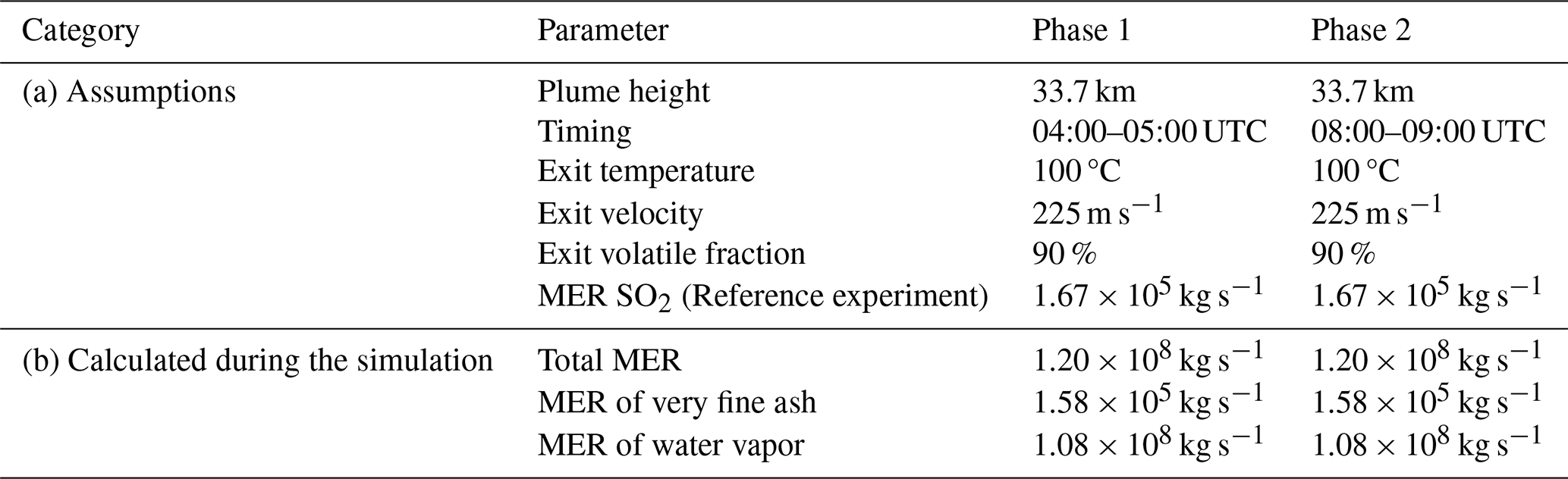
The input parameters used for FPlume for the eruption phases are summarized in Table 1. We chose the same values for both eruption phases, as the uncertainty range of the measurement is large and detailed information on plume dynamics during both phases is lacking. Furthermore, we used a plume top height of 33.7 km, which is in the uncertainty range of observations of the umbrella plume (neglecting the overshooting top) (e.g., Gupta et al., 2022) and also ensures that approximately 150 Tg of water vapor remains in the stratosphere after the emission (phase transition depends on temperatures and, therefore, the injection height). In our simulations, about 500 Tg of solid hydrometeors (ice and snow) and less than 50 Tg of liquid hydrometeors (cloud and rain water) are released into the stratosphere, which subsequently fall out in the first 1–2 d.

Table 1 Summary of the assumptions (a) and FPlume-derived MERs (b). The plume heights for the umbrella top heights are from Gupta et al. (2022). The MER of SO₂ was derived from the total mass of 1.2 Tg SO₂ after the eruption (Sellitto et al. (2022, 2024) estimated an emission of more than 1.0 Tg). The values for the exit temperature, exit velocity, and exit volatile fraction were taken from Mastin et al. (2024).

2.2 Model setup and experiments

We performed seven experiments to investigate the role of water vapor, ash, and aerosol dynamics in the first week after the Hunga eruption. The assumptions for the experiments are summarized in Table 2. All simulations were performed globally using a horizontal grid spacing of approximately 40 km (R02B06) and 90 vertical levels resolving the atmosphere up to a height of 75 km. For each experiment, we simulated 7 d initialized on 15 January 2022 at 00:00 UTC with analysis data provided by the German Weather Service (DWD). The analysis data contained variables describing the atmospheric state, variables needed by the land component, and sea surface temperatures. Due to the short time span of the simulation, the sea surface temperatures are temporally fixed throughout the simulation.

Table 2 Experiments performed for this study.

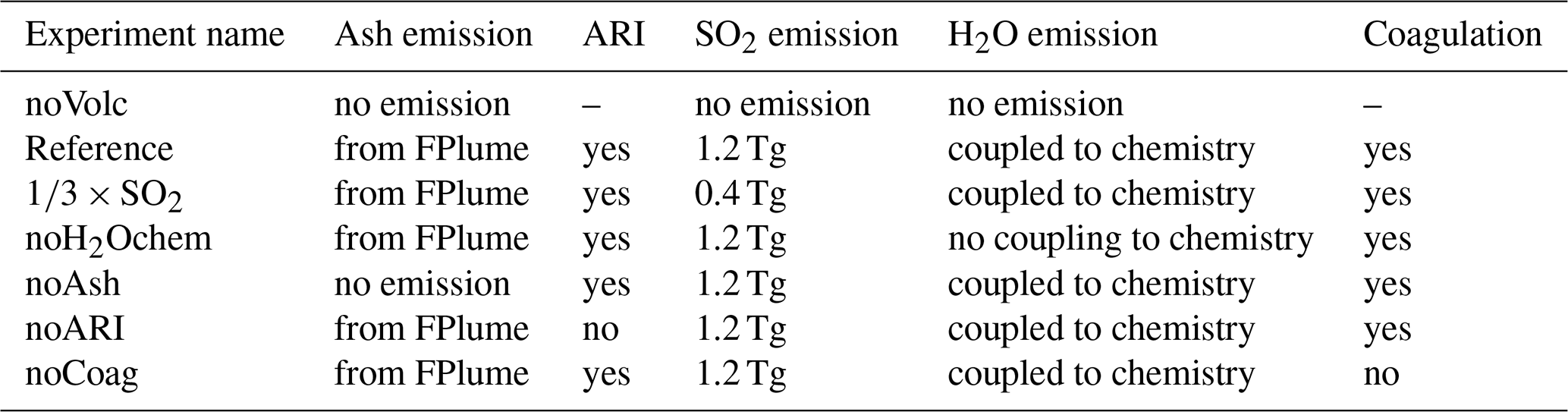
The first estimate of the SO₂ mass in Carn et al. (2022) was on the order of 0.4–0.5 Tg. We therefore used 0.4 Tg in the experiment $\mathrm{1}/\mathrm{3}$ × SO₂, similar to the modeling study by Zhu et al. (2022). However, Sellitto et al. (2022) argued that the measurements might have underestimated the SO₂ concentration on the first day. Based on their analysis, Sellitto et al. (2022) proposed a value of at least 1 Tg SO₂ entering the stratosphere during the eruption. Thus, for the experiments Reference, noH₂Ochem, noARI, noAsh, and noCoag, we tripled the SO₂ emission compared to the experiment $\mathrm{1}/\mathrm{3}$ × SO₂.

The mass of very fine ash was evenly distributed into the three insoluble modes (accumulation, coarse, and giant mode), with median diameters of 0.8, 2.98, and 11.35 µm, respectively, and a standard deviation of 1.4 (Muser et al., 2020). The emission of the number density is derived from the emitted mass and the definition of the log-normal distributions.

The observed umbrella radius was expanding to about 80 km (Carr et al., 2022) at 04:30 UTC. Therefore, we distributed the emissions horizontally into 10 cells covering an area of approximately 16 000 km³, which is equivalent to the area covered by a circle with a radius of 71 km.

2.3 Observations and methods

In this study, we used observations from the CALIOP instrument for the validation of the aerosol and hydrometeor transport, Ozone Mapping and Profiler Suite (OMPS) SO₂ column loadings for the validation of SO₂ oxidation and transport, and Infrared Microwave Sounding/Infrared Atmospheric Sounding Interferometer (IMS/IASI) sulfate aerosol optical depth (SAOD) for the validation of the sulfate formation and transport.

2.3.1 CALIOP

The CALIOP instrument on board the CALIPSO (Cloud-Aerosol Lidar and Infrared Pathfinder Satellite Observations) satellite has provided high-resolution vertical profiles of aerosols and clouds since May 2016. The measurements are based on the backscattered signal at 532 and 1064 nm. Two channels receive orthogonally polarized components of the 532 nm backscattered signal, whereas the 1064 nm backscatter intensity is received only at one channel (Winker et al., 2009). We used total attenuated backscatter (ATB) signals and depolarization ratios at 532 nm from the CALIOP instrument to validate the simulated aerosol plume transport.

The ICON-ART ATB signals were calculated offline from simulated aerosol mass mixing ratios with the forward operator described in Hoshyaripour et al. (2019) and applied to volcanic plumes in Bruckert et al. (2023). In total, nine CALIPSO overpasses traversed the Hunga plume within the first week after the eruption.

2.3.2 OMPS

We validated the modeled transport and SO₂ oxidation with SO₂ column loadings from the OMPS nadir mapper (NM). OMPS is an ultraviolet (UV) satellite sensor on the Suomi-National Polar-orbiting Partnership (Suomi-NPP) satellite by the National Aeronautics and Space Administration (NASA) and the National Oceanic and Atmospheric Administration (NOAA) that has been operating since 2011 (Carn et al., 2015). It measures the backscattered UV radiance spectra between wavelengths of 300 and 380 nm with a spectral resolution of 1 nm. The instrument provides a daily global coverage, which is achieved with a 2800 km cross-track swath with a nadir pixel size of 50 km × 50 km (Carn et al., 2015).

2.3.3 IMS/IASI

IASI is a nadir-viewing infrared Fourier transform spectrometer on the MetOp A, B, and C satellites that provides spectra at 0.5 cm⁻¹ apodized resolution, sampled every 0.25 cm⁻¹ from 625 to 2760 cm⁻¹ (Blumstein et al., 2004). Spectra are measured with four detectors, each with a circular field of view on the ground (at nadir) of approximately 12 km in diameter, arranged in a 2 × 2 grid within a 50 × 50 km² field-of-regard (FOR). IASI scans to provide 30 FOR (i.e., 120 individual spectra) evenly distributed across a 2200 km wide swath. MetOp is in sun-synchronous polar orbit with a local time of descending node crossing of 09:30. It therefore provides almost complete global coverage twice per day at 09:30 and 21:30 local time.

The Rutherford Appleton Laboratory (RAL) IMS scheme employs the optimal estimation method (Rodgers, 2000) to jointly retrieve atmospheric and surface parameters from IASI (in combination with the microwave sounders also on MetOp) (Siddans, 2023). The scheme uses the RTTOV 12 (Radiative Transfer for the TIROS Operational Vertical Sounder (TOVS)) radiative transfer model (Saunders et al., 2017) to simulate measured spectra, including the effects of aerosol. IMS retrieves the SAOD at 1170 cm⁻¹ (8.5 µm) (i.e., at the peak of the sulfate aerosol mid-infrared extinction cross section), making the following assumptions to define the profile shape and optical properties: (1) the aerosol extinction coefficient profile is assumed to have a Gaussian shape that peaks at an altitude of 20 km, with a 1 km full-width-half-maximum. (2) The sulfate droplet aerosol type at 0 relative humidity from Hess et al. (1998) is assumed to define the aerosol size distribution and optical properties. IMS SAOD has been used in previous studies of the Hunga plume (e.g., Sellitto et al., 2022; Legras et al., 2022; Sellitto et al., 2024). The data are gridded to a 0.25°x0.25° spatial sampling in hourly time intervals.

2.4 SAL analysis

The Structure-Amplitude-Location (SAL) method, developed by Wernli et al. (2008, 2009) for the validation of modeled and observed precipitation fields, is applied to validate our modeled SO₂ column loadings and sulfate aerosol optical depth (SAOD) against observations. The equations for the calculation of the SAL components are given in Wernli et al. (2008).

The SAL method analyzes the agreement of objects in two-dimensional data fields according to three components: structure, amplitude (A), and location (L). S compares modeled and observed normalized objects with respect to their volume. It can have values between −2 (modeled objects are too small and/or too peaked) and 2 (modeled objects are too large and/or too flat). A value of 0 indicates a perfect agreement between model and observations with respect to the structure. The evaluation of the domain-averaged relative deviation of the modeled fields from observations is given by the component A. Similar to the S component, A varies between −2 (model underestimates the predicted quantity) and 2 (model overestimates the predicted quantity), with a perfect agreement if A is 0. The agreement in location is given by the component L and is the sum of two steps: first, the agreement between the forecast and observation in terms of the normalized difference between the centers of mass is calculated. Second, the average distance between the center of mass of all objects and the individual objects is derived. Each step can reach values between 0 and 1, so L in total ranges from 0 to 2, with a perfect forecast with respect to the location at L = 0 (Wernli et al., 2008, 2009).

For the SAL validation of modeled SO₂ column loadings with observations, we used the OMPS data. We applied the OMPS detection threshold of 0.2 DU (Li et al., 2017) on both the observational and modeled data field. As the OMPS data are organized into overpasses, we mapped the data as follows for the SAL comparison: for every overpass, we first chose the corresponding ICON-ART output dataset and checked whether the plume is detected in both fields. If yes, we mapped the overpass area for model and observations onto a 0.25° × 0.25° grid. If the plume was detected in the subsequent overpasses as well, we combined these overpasses into one map. In total, we received seven mapped fields containing the plume in the first week after the eruption for the comparison with OMPS (Fig. C1).

For the comparison with the IMS/IASI SAOD, the ICON-ART SAOD was calculated offline from the mass concentration m_l in kg m⁻³ of the two soluble modes l and their respective mass extinction coefficients $k_{i,\mathrm{1130}{\mathrm{cm}}^{-\mathrm{1}}}$ derived from Mie calculations for 1130 cm⁻¹:

$$\begin{array}{}\text{(1)}& {\mathit{\tau }}_{\mathrm{1130}{\mathrm{cm}}^{-\mathrm{1}}}=\sum _{i=\mathrm{1}}^z\sum _{l=\mathrm{1}}^{\mathrm{2}}{m}_l\cdot k_{i,\mathrm{1130}{\mathrm{cm}}^{-\mathrm{1}}}\cdot \mathrm{\Delta }{z}_i,\end{array}$$

with z being the model level. We performed a comparable procedure with ICON-ART SAOD and IMS/IASI SAOD data for the SAL validation of the sulfate mass, similar to the approach used for the SO₂ column loading. The differences relative to the procedure with the OMPS SO₂ column loading data are that the IMS/IASI data have already been mapped to a 0.25° × 0.25° grid for each overpass and that the background of the SAOD observations is much busier and thus it is more difficult to distinguish the plume. Therefore, we used a threshold of 0.01 for the SAOD model and observational data and additionally checked whether the SO₂ Hunga plume was available in the same grid cell in the IASI data. In total, 12 mapped fields containing the plume were detected (Fig. C2).

3 Drivers of in-plume chemistry and microphysics

In this section, we aim to investigate the role of ARI, water vapor, and ash emission on the oxidation of SO₂ and the formation of sulfate aerosols and ash aging.

3.1 Impact of water vapor and SO₂ emissions

Previous work has already shown a faster oxidation of SO₂ in the Hunga plume due to the additional emission of water vapor (e.g., Sellitto et al., 2022; Zhu et al., 2022; Asher et al., 2023). Therefore, we focus on the effects of water vapor emission and SO₂ amount on the microphysical developments in the first hours of the plume (i.e., focus on the experiments $\mathrm{1}/\mathrm{3}$ × SO₂, noH₂Ochem, and Reference) and compare our results to existing studies. Figure 1 shows the temporal mass development of SO₂, sulfate, the water on aerosols, ash, water vapor, and OH.

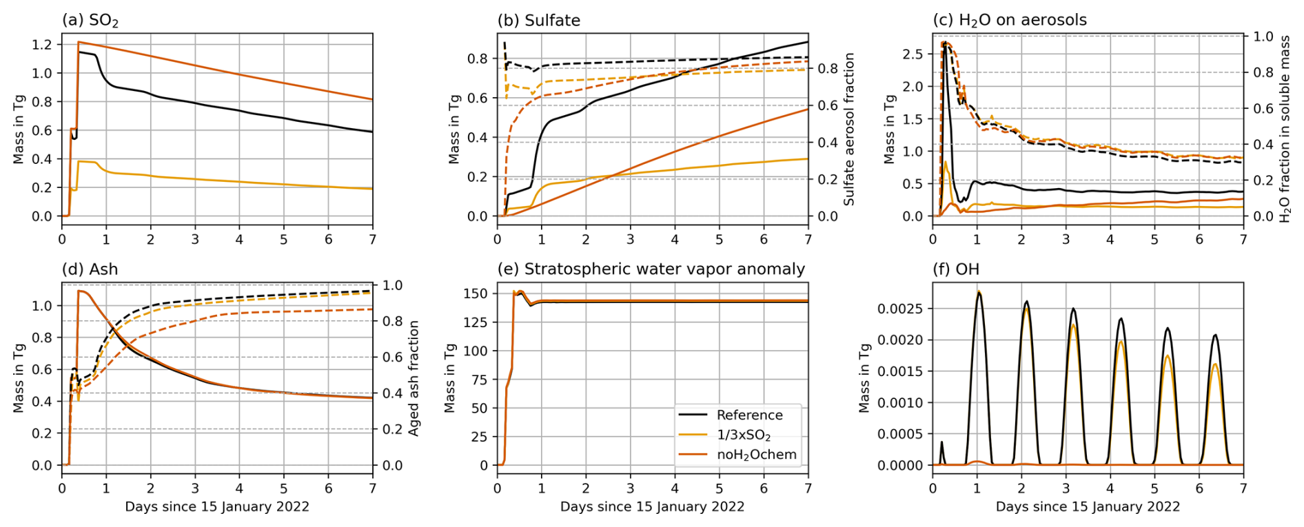
Figure 1 Temporal plume mass development (solid lines, left y axis) of (a) SO₂, (b) sulfate aerosols plus sulfate on coated ash, (c) liquid water in sulfate aerosols plus liquid water on coated ash, (d) ash, (e) stratospheric water vapor anomaly, and (f) OH for the experiments Reference, $\mathrm{1}/\mathrm{3}$ × SO₂, and noH₂Ochem. The dashed lines (right y axis) indicate fractions of (b) sulfate aerosol mass divided by total sulfate mass, (c) water mass divided by the sum of water and sulfate mass, and (d) aged ash mass divided by total ash mass.

The co-emission of water vapor accelerates the oxidation of SO₂ and the formation of sulfate aerosols (compare the $\mathrm{1}/\mathrm{3}$ × SO₂ and noH₂Ochem experiments in Fig. 1a and b), which agrees with the findings by Zhu et al. (2022). The faster SO₂ oxidation in the presence of the water vapor plume is caused by the increase in OH radicals (Fig. 1f) produced via water vapor and ozone chemistry in the stratosphere.

All experiments with H₂O contribution to chemistry show a strong reduction of SO₂ in the last quarter of the first day, whereas the experiment noH₂Ochem reveals a linear decrease (Fig. 1a) within the first week. This strong decrease is due to both the high water vapor concentration in the plume shortly after the emission and the onset of the OH production by photolysis (Fig. 1a and f).

The experiment $\mathrm{1}/\mathrm{3}$ × SO₂ shows a significantly smaller formation of sulfate because less SO₂ is available for oxidation (Fig. 1a and b). A larger sulfate formation leads to more water accumulation on aerosols (compare the experiments $\mathrm{1}/\mathrm{3}$ × SO₂ and Reference in Fig. 1b and c). The H₂O fraction in soluble mass (Fig. 1c, right y axis) was calculated as the mass of H₂O in aerosols divided by the mass of H₂O and sulfate in aerosols. The fraction peaks during the first hours when the water vapor concentration is highest (i.e., during the emission) and decreases over time. Thus, the fraction of sulfate increases in the soluble mixture. The soluble mass after 1 week is composed of roughly $\mathrm{2}/\mathrm{3}$ sulfate and $\mathrm{1}/\mathrm{3}$ H₂O, with small differences between the experiments shown in Fig. 1.

Satellite instruments detected ash on the first day after the eruption; however, it was not detectable in the following days. In the next section, we investigate whether ash played a role in the plume development during the first hours after the eruption and whether aerosol aging, accelerated by the fast SO₂ oxidation, explains why satellites could not detect ash during the further transport.

3.2 Impact of ash and the aerosol–radiation interaction

ARI can increase the scattering of sunlight (e.g., Robock, 2000; Timmreck, 2012) and can reduce photolysis in volcanic plumes. Ash aerosols can coagulate with sulfate or provide surfaces for H₂SO₄ condensation, resulting in the aging of volcanic ash and lower amounts of sulfate aerosols. In this section, we discuss the role of ash and ARI on the development of the Hunga plume. Therefore, we focus on the experiments Reference, noARI, noCoag, and noAsh in Fig. 2, i.e., the experiments with larger SO₂ emission and with volcanic water vapor contribution to chemistry.

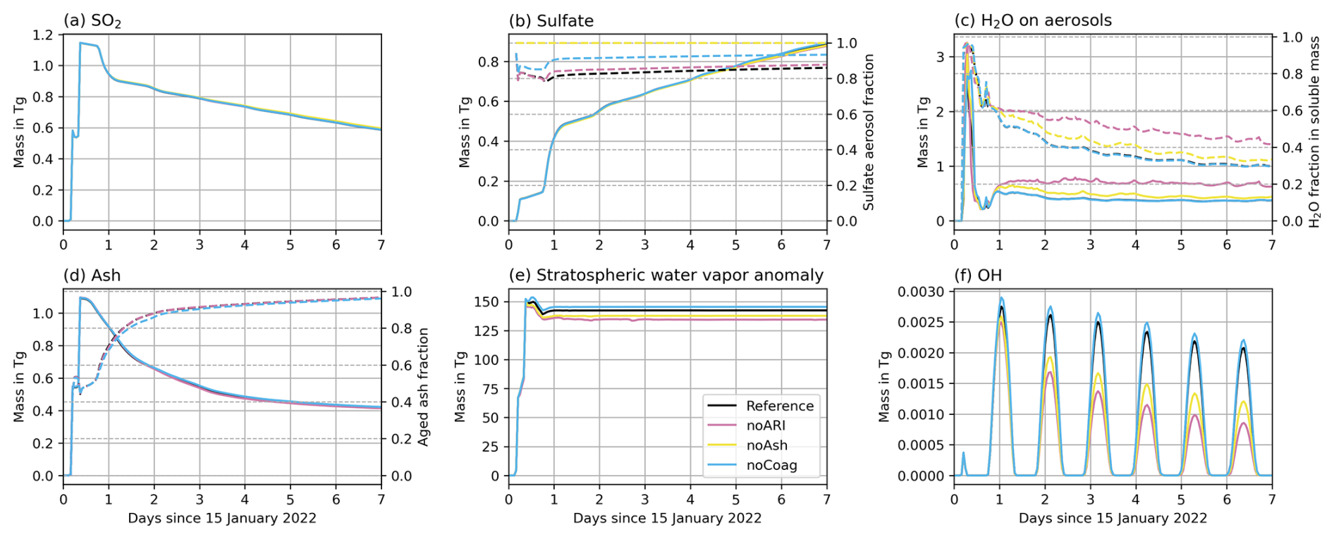
Figure 2 Same as Fig. 1 but for the experiments Reference, noARI, noCoag, and noAsh. Note that the curves in (a), (b), and (d) are overlapping.

ARI decreases the oxidation of SO₂ in the Hunga plume only very slightly (Fig. 2b, compare noARI and Reference). Determining the pure effect of the reduction in sunlight on the SO₂ oxidation is difficult to model in a physically consistent way, as ARI causes a lofting of the plume to layers with larger ozone concentrations. A higher concentration of ozone can increase the SO₂ oxidation, which represents an opposing effect to the reduction of sunlight by ARI, i.e., the pure effect of the blocking of sunlight by aerosols might be larger than the ARI effect visible in Fig. 2b.

The presence of ash particles in the plume results in a slightly lower fraction of sulfate aerosols relative to the total sulfate mass (dashed lines in Fig. 2b, compare the Reference and noAsh experiments), as ash particles provide surfaces for H₂SO₄ condensation and coagulation. This leads to aging or coating of the ash, which occurs a bit more quickly when more SO₂ is emitted (dashed lines in Fig. 1d, see the Reference and $\mathrm{1}/\mathrm{3}$ × SO₂ experiments). In all experiments, except noH₂Ochem, more than 90 % of the ash mass in the plume is coated after less than 3 d (dashed lines in Figs. 1d and 2d). Ash aging is slower without volcanic water vapor contribution to chemistry (dashed line in Fig. 1d for noH₂Ochem). Nevertheless, more than 80 % of the ash is aged after 1 week in the experiment, despite the smaller oxidation of SO₂. Comparing the curve for the sulfate aerosol fraction of the noH₂Ochem experiment with the curves of the $\mathrm{1}/\mathrm{3}$ × SO₂, Reference, and noARI experiments, we can conclude that sulfate tends to form a coating on ash particles rather than creating uniform sulfate particles (Figs. 1b and 2b). The early aging of ash mainly happens through condensation of soluble components (e.g., sulfate and/or water) rather than coagulation of ash with sulfate aerosols (compare dashed lines for Reference and noCoag in Fig. 2d).

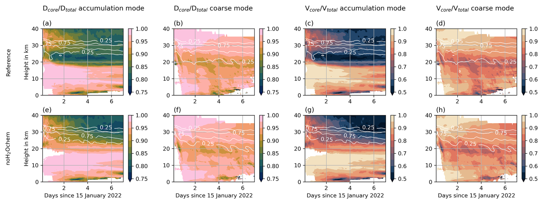
Figure 3 Coating fraction in the Reference experiment (top row) and the noH₂Ochem experiment (bottom row) based on the fraction of core to total particle diameter (first and second columns) and based on the fraction of core to total particle volume (third and fourth columns) in color. The first and third columns refer to the mixed accumulation mode, and the second and fourth columns refer to the mixed coarse mode. The white contour lines refer to the fraction of maximum aerosol concentrations and indicate the vertical distribution of the plume.

Figure 3 shows the coating fraction based on particle diameter (first and second columns) and particle volume (third and fourth columns) of the mixed accumulation (first and third columns) and the coarse (second and fourth columns) mode for the Reference (top row) and the noH₂Ochem (bottom row) experiment. In addition to a larger fraction of aged particles, as discussed before, the coating itself on ash particles also increases with water vapor emission. The differences in coating fraction between the two experiments is largest for the accumulation mode between 20 and 25 km, where the shell makes up about 20 % by diameter or about 50 % by volume of the particles (compare Fig. 3a and e or c and g). For the coarse mode particles, the coating fraction is larger after about 3 d at the altitude where the sedimentation of particles becomes visible, i.e., below 20  km (Fig. 3b and f or d and h).

Although ash aging is faster when large amounts of water vapor are available in the plume, the coating is not large enough to remove a majority of the ash within the first day, as was proposed by satellite observations (e.g., Legras et al., 2022). One reason for the discrepancy between our model results and satellite observations could be that coated ash, which tends to be more spherical compared to the uncoated ash, was interpreted as sulfate by the satellite algorithm. Another reason could be that we miss one or more important aerosol dynamical processes in our current model setup, such as the coagulation of ash with sea salt injected into the stratosphere by the eruption (Colombier et al., 2023). Sea salt is more hygroscopic than sulfate and might increase the water uptake on aged ash particles, which leads to a faster growth and removal by sedimentation. The neglected activation of ash or the missing wet aggregation in the plume in our model setup might also explain the discrepancy between our simulations and observations. However, the role of sea salt in the Hunga plume on aerosol dynamical processes and the effects of aggregation and activation are beyond the scope of this study and are the topic of another ongoing investigation.

Considering ARI leads to a soluble mass that is composed of roughly $\mathrm{2}/\mathrm{3}$ sulfate and $\mathrm{1}/\mathrm{3}$ H₂O with small differences between the experiments (Fig. 1c and 2c). For the experiment noARI, the fraction of H₂O in aerosols is higher (roughly 40 %). The reason might be that the plume is transported at lower altitudes in noARI, where the temperatures in the plume are lower and the relative humidity is larger (Fig. B1).

The water vapor development in the plume shows small differences due to ARI (Fig. 2e, compare Reference and noARI), which leads to a warming of the surrounding air and a lofting of the plume to warmer stratospheric layers (Muser et al., 2020). However, the amount of ash in the Hunga plume is too small to significantly heat the plume and reduce the rate of ice formation in the initial phase of the eruption (Figs. 1e and 2e). The effect of ARI is discussed in more detail in the following.

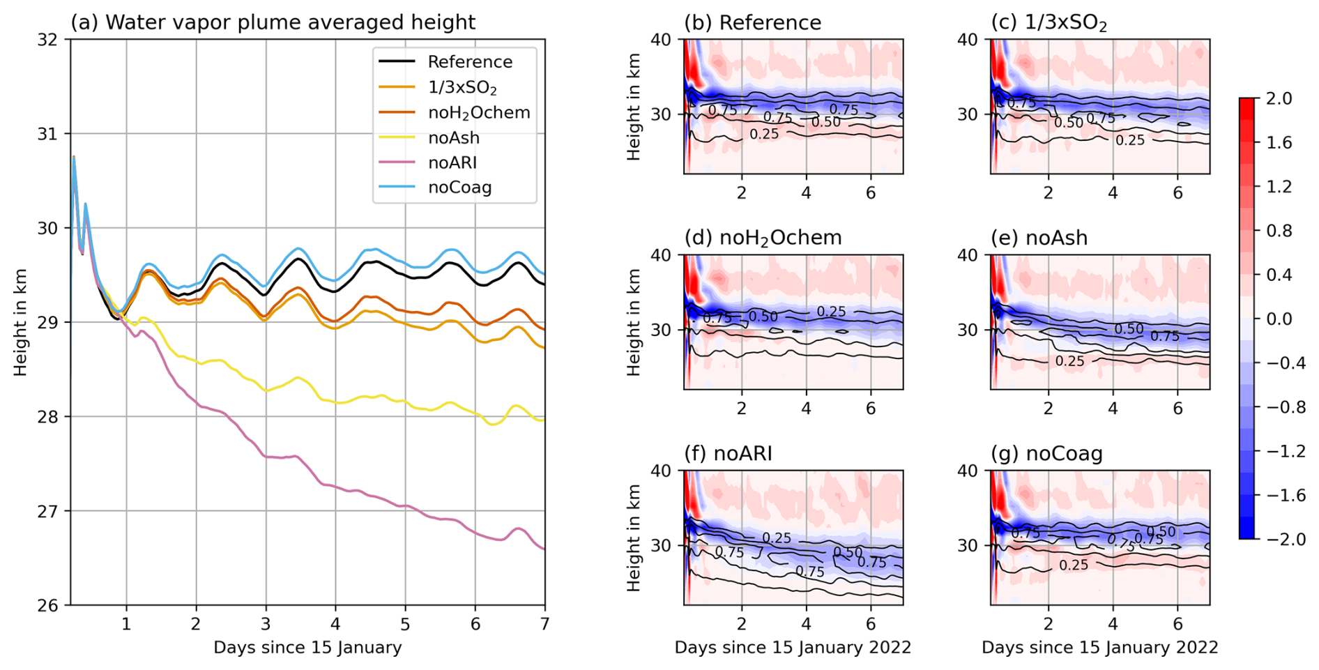
Figure 4 (a) Temporal evolution of the mass-averaged water vapor plume height, and (b–g) plume temperature anomaly (in K, various colors) and fraction of maximum volcanic water vapor concentrations (black contours) for the different experiments.

Figure 4 shows the mass-averaged height of the water vapor plume in the different experiments in (a) and the temperature anomaly of the experiments in (b)–(g). The experiment noARI shows a decrease of more than 3 km within the first week (Fig. 4a) due to water vapor cooling in the stratosphere (Fig. 4f). The experiments including ARI also reveal a negative temperature anomaly from about 28 to 33 km coinciding well with the position of the water vapor plume (Fig. 4b–e and g). However, the descent of the water vapor is reduced (in the noAsh experiment), balanced out (in the Reference, noH2Ochem, and $\mathrm{1}/\mathrm{3}$ × SO₂ experiments), or even opposed (in the noCoag experiment) after the first day by the warming due to ARI.

All experiments show a steep decrease in the water vapor plume averaged height during the first day (Fig. 4a). The reasons are (1) a large concentration of water vapor during and in the first few hours after the emission leading to strong radiative cooling, (2) the absence of sunlight during the night (emission at 17.00–18.00 and 21.00–22.00 local time), and (3) the strong formation of sulfate starting after the first day.

The reduction in descent rate after the first day is due to both sulfate and ash interaction with radiation. Ash contributes approximately $\mathrm{2}/\mathrm{3}$ (compare Reference and noAsh in Fig. 4a) and sulfate contributes about $\mathrm{1}/\mathrm{3}$ (compare noARI and noAsh in Fig. 4a) to the decrease in descent rate.

The experiment noCoag shows the smallest descent rate for the water vapor plume (Fig. 4a, blue curve) because coagulation decreases the number concentration of particles and increases the radii. Neglecting this process changes the interaction of aerosols with radiation, consequently affecting the plume temperatures and lofting. For particles of the same composition but different size, the smaller particles interact more strongly with radiation in the visible range. This increases the warming and lofting of the plume in the noCoag case, which also affects the mass-averaged height of the water vapor plume (Fig. 4a and g).

Khaykin et al. (2022) found a descent rate of the plume on the order of 200 m d⁻¹ during the first 3 weeks in water vapor observations with the Microwave Limb Sounder (MLS; maximum plume top altitudes decreasing from near 30 km between 16 and 19 January to about 26 km between 1 and 10 February). Together with our finding in noARI, we argue that ARI is necessary to reproduce the observed plume descent. However, our simulations with ash seem to underestimate the ash removal, which leads to an overestimation of the radiative warming by aerosols and an underestimation of the water vapor descent. The descent rate of water vapor in the experiment noAsh is closest to the descent observed by Khaykin et al. (2022).

Stenchikov et al. (2024) found a descent from 35 to 27 km in the first 2 weeks in model simulations, which is even stronger than in our noAsh experiments. The discrepancy relative to our results is likely to be attributed to differences in the emission assumptions and the lower vertical resolution of the model in Stenchikov et al. (2024). Particularly, differences in the vertical emission profile, emission timing, and horizontal emission area affect the concentration of water vapor in the initial phase and, consequently, the interaction with radiation.

Positive temperature anomalies arise in all experiments in the first hours after the eruptions above 33 km (Fig. 4b–g). This is an effect of microphysical processes (mainly ice formation) in the plume during the emission (not shown).

4 Validation of model results

In this section, we focus only on the experiments Reference, noH₂Ochem, and $\mathrm{1}/\mathrm{3}$ × SO₂, as the other experiments show only small differences with respect to the Reference case regarding the masses of aerosols and SO₂ (Sect. 3). These differences are not distinguishable in the comparison to the observations (not shown).

4.1 SAL analysis to validate SO₂ oxidation and sulfate formation

We performed an SAL analysis to validate the modeled SO₂ oxidation with OMPS observations (SO₂ column loadings) and modeled sulfate formation with IMS/IASI observations (SAOD). The results are shown in Fig. 5 for the experiments Reference (left), noH₂Ochem (middle), and $\mathrm{1}/\mathrm{3}$ × SO₂ (right).

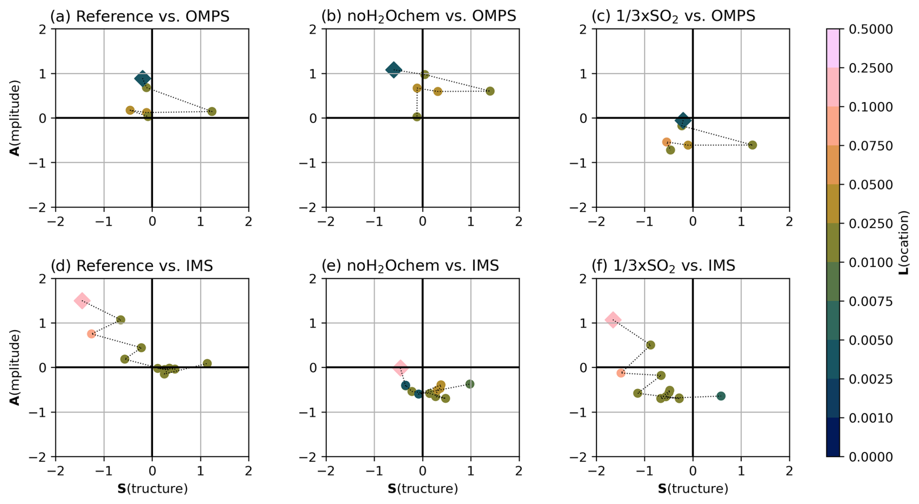
Figure 5 SAL analysis between ICON-ART and OMPS SO₂ column loadings (a–c) and between ICON-ART and IMS SAOD (d–f) for the experiments Reference (left column), noH₂Ochem (middle column), and $\mathrm{1}/\mathrm{3}$ × SO₂ (right column). The structure value is given on the x axis, the y axis shows the amplitude value, and the location value is indicated by different colors. Each symbol in the plot refers to one comparison date, with the square symbol indicating the first comparison and subsequent comparisons being connected by the dashed line. The corresponding dates and mapped SO₂ column loadings and SAODs are given in Figs. C1 and C2.

The best agreement between model and observations with respect to both SO₂ and sulfate is achieved in the Reference simulation (Fig. 5a and d). Especially in the latter half of the simulation, all values are close to 0 for both SO₂ and sulfate. In the first days, the amplitude value is around 1 for both compounds, which might indicate an overestimation of the variables by the model. However, during the first days, a thick ice and ash plume was visible (e.g., Legras et al., 2022), which might have masked SO₂ and sulfate in the observations. Furthermore, OMPS might not have detected the SO₂ plume well in the first days because of insufficient sampling.

Neglecting the effect of volcanic water vapor on chemistry leads to an underestimation of the SO₂ oxidation, i.e., an overestimation of the SO₂ column loadings (Fig. 5b). Additionally, the SAOD and, thus, the sulfate formation were underestimated by the model in the latter half of the simulation in the noH₂Ochem experiment.

Although the $\mathrm{1}/\mathrm{3}$ × SO₂ experiment reveals a reasonable agreement with respect to all SAL components for the SO₂ column loadings in the first half of the simulation, it clearly underestimates the formation of sulfate after the eruption and the SO₂ column loadings in the second half of the simulation (Fig. 5c and f). This indicates that the SO₂ mass was larger than the initial estimate of 0.4 Tg by Carn et al. (2022) and was approximately 2 to 3 times larger (Sellitto et al., 2022, 2024, and Fig. 5a).

The location values for all experiments are slightly better for SO₂ column loadings than for SAOD because the SO₂ plume can be more distinctly separated from background SO₂ than the sulfate can. Nevertheless, the location values indicate a good agreement between model and observations for all times, both components, and all experiments.

4.2 CALIPSO overpasses to validate transport and composition

We analyzed nine Hunga plume overpasses by the CALIPSO satellite and compared the ATB from CALIOP with the Reference, $\mathrm{1}/\mathrm{3}$ × SO₂, and noH₂Ochem experiments as well as the CALIOP depolarization ratio with the spherical fraction ((sulfate mass + aged ash mass)/total aerosol mass) and the sulfate fraction (sulfate mass/total aerosol mass) of the experiments. Figures 6 and 7 show two examples; the seven other overpasses can be found in Appendix D1–D7.

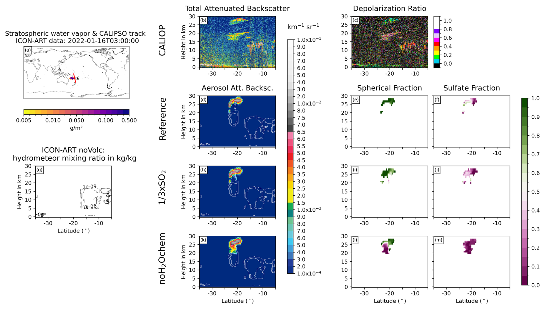
Figure 6 Comparison of ICON-ART and CALIOP for the overpass on 16 January 2022 at 03:00 UTC. (a) shows the stratospheric water vapor column loadings anomaly from ICON-ART, with the CALIPSO track shown as a red line and the location of the volcano shown as a black triangle. The second column compares CALIOP total ATB at 532 nm (b) to ICON-ART aerosol ATB (in different colors) for the experiments Reference (d), $\mathrm{1}/\mathrm{3}$ × SO₂ (h), and noH₂Ochem (k). The white contours refer to the normalized mixing ratios of ICON-ART hydrometeors, indicating the positions of clouds in the model. Panel (g) refers to the mixing ratio of hydrometeors from the simulation noVolc without volcanic eruption in order to distinguish background meteorological clouds from clouds produced by the volcanic emission of water vapor. The third column shows the CALIOP depolarization ratio (c) and ICON-ART fraction of spherical particle mass (mass of sulfate and aged ash divided by total aerosol mass) for the experiments Reference (e), $\mathrm{1}/\mathrm{3}$ × SO₂ (i), and noH₂Ochem (l), respectively. The fourth column shows the ICON-ART sulfate fraction, defined as the mass of sulfate aerosol divided by the total mass of aerosols, for the experiments Reference (f), $\mathrm{1}/\mathrm{3}$ × SO₂ (j), and noH₂Ochem (m), respectively.

The overpass on 16 January 2022 at 03:00 UTC indicates two plumes at (1) 15–20 km and (2) 27–30 km (20–30 km for noH₂Ochem) at about 23 to 27° S in the CALIOP and ICON-ART ATB (Fig. 6b, d, h, k). The upper signal consists of spherical particles (indicated by the blue-greenish colors in Fig. 6c), and it is well reproduced by the aerosol ATB by the ICON-ART experiments Reference and $\mathrm{1}/\mathrm{3}$ × SO₂. The ICON-ART spherical and sulfate fractions of the Reference and $\mathrm{1}/\mathrm{3}$ × SO₂ experiments indicate that this plume is dominated by spherical particles consisting of both aged ash and sulfate (Fig. 6e, f, i, and j). For the noH₂Ochem experiment (Fig. 6k and i), the upper signal reaches lower altitudes, and the plume is dominated by non-spherical particles. Thus, without the effect of volcanic water vapor on chemistry, the satellite observations cannot be reproduced.

The lower signal in the CALIOP ATB most likely originates from ice formed from the Hunga volcanic water vapor because it is visible in the hydrometeor mixing ratios in all three experiments including volcanic emissions (white contours in Fig. 6d, h, and k) but is absent in the experiment without volcanic emission (Fig. 6g). The CALIOP depolarization ratio further supports that this signal comes from non-spherical particles such as ice or uncoated ash (indicated by reddish colors in Fig. 6c).

All ICON-ART experiments (with and without volcanic eruption) indicate hydrometeors in the background north of 17° S, and their positions agree reasonably well with the positions of the signals in the CALIOP total ATB.

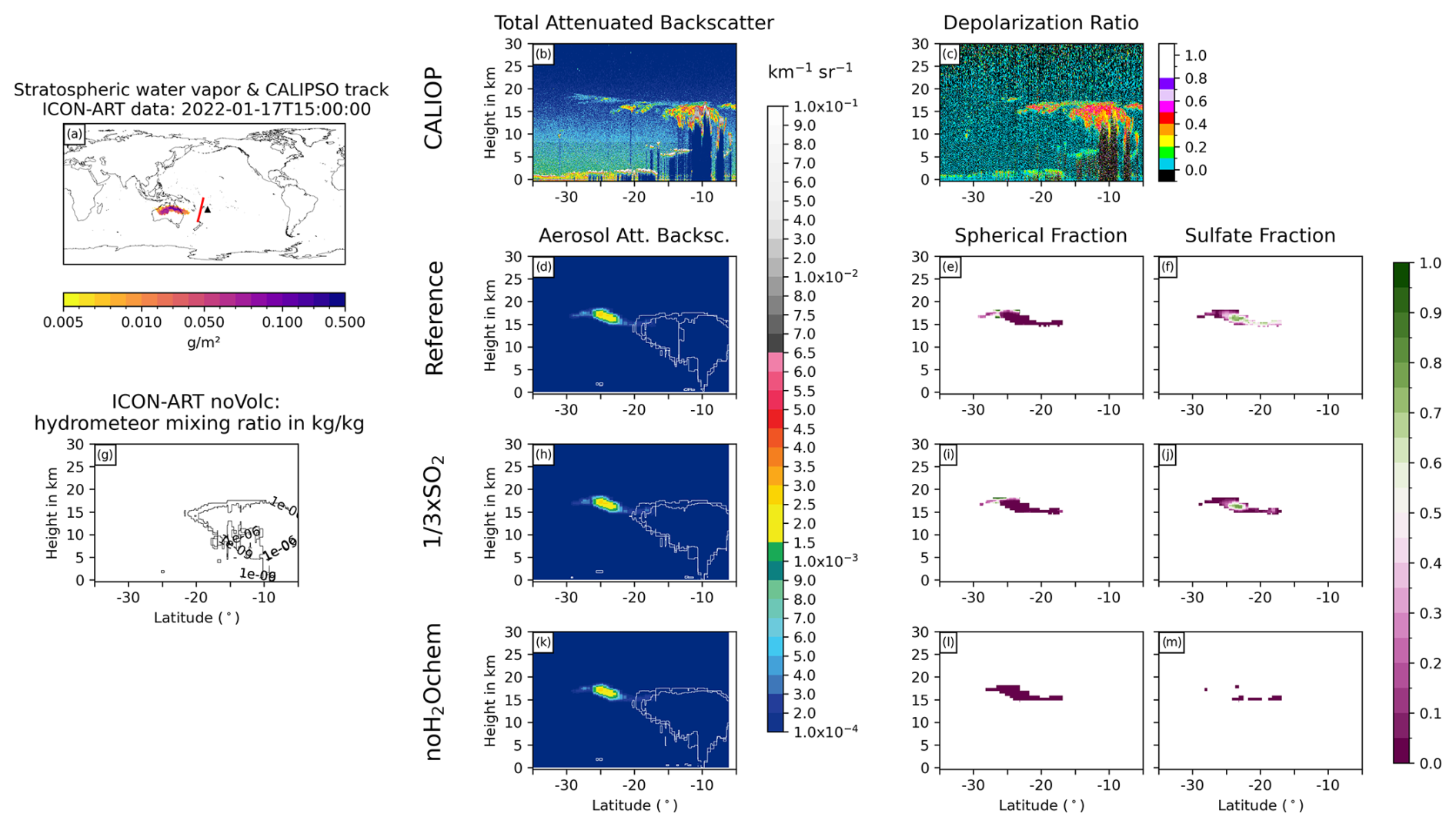
Figure 7 Same as Fig. 6 but for 17 January 2022 at 15:00 UTC.

The overpass on 17 January 2022 at 15:00 UTC shows a layer of non-spherical particles from 5 to 27° S in the CALIOP measurements at the tropopause (about 18 km), which is only thin at the southern half (less than 3 km thick) and reaches down to 10 km north of 17° S (Fig. 7b and c). The northern part most likely arises due to hydrometeors in the background and is visible in all experiments (contour lines in Fig. 7d, g, h, and k). The southern part, especially south of 20°S, reveals no clouds in the ICON-ART experiments but does show non-spherical aerosol particles (Fig. 7d–m). We therefore argue that this signal in the CALIOP total ATB with a relatively large depolarization ratio (i.e., non-spherical particles) originates from uncoated ash instead of ice clouds. Nevertheless, the amplitude of the aerosol ATB is slightly overestimated by ICON-ART (Fig. 7b, d, h, and k).

All in all, the comparison to the CALIOP data reveals that parts of the “missing” ash in satellite data might be hidden due to a strong coating in the presence of volcanic water vapor. However, the simulated aerosol ATB signals tend to overestimate the observed total ATB signals, which agrees with our argumentation in Sect. 3.2 that we miss important removal processes in our current model setup. Furthermore, the comparison shows that ice particles are present in the plume in both the models and observations on the first day after the eruption, but the ice was quickly removed, which is in agreement with observations (e.g., Legras et al., 2022; Sellitto et al., 2022).

5 Development of particle sizes

Several measurements show a growth of sulfate particles in the first weeks after the eruption (e.g., Kloss et al., 2022; Asher et al., 2023; Boichu et al., 2023). In this section, we investigate the simulated evolution of the particle size and compare it to previous studies, after which we discuss the contribution of the different processes to the particle evolution.

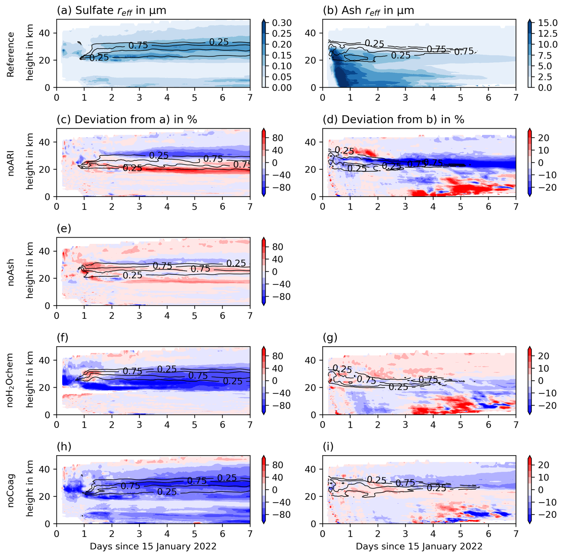
Figure 8 Temporal development of the plume-averaged effective radii for sulfate aerosols (left) and ash aerosols (right) in the Reference experiment (first row), and the deviation from the Reference experiment for the experiments noARI (second row), noAsh (third row), noH₂Ochem (fourth row), and noCoag (fifth row) in different colors. The black contour lines indicate the fraction of maximum aerosol concentrations for the sulfate (left column) and ash plume (right column), respectively, in order to visualize the vertical distribution of the plume.

Figure 8 shows height-time cross sections of the sulfate and ash effective radii for the Reference experiment (top row) and deviations from the Reference experiment for the noARI, noAsh, noH₂Ochem, and noCoag experiments. The values are horizontally averaged over the entire plume. The sulfate effective radius increases over time during the first week after the eruption by a factor of about 2 to 3 (Fig. 8a), which has also been found in observations (e.g., Asher et al., 2023; Boichu et al., 2023; Randel et al., 2023). The maximum effective sulfate radius after 1 week is about 0.35 µm, which agrees well with the value after 1 week by Stenchikov et al. (2024).

The ash effective radius decreases fast during the first 3 d, as the larger particles sediment faster than the smaller ones. After 1 week, the ash effective radius is smaller than 4 µm on average (Fig. 8, left side). Boichu et al. (2023) found particles with peak radii larger than typical sulfate particle sizes at one AERONET station and argued that these particles might be sulfate-coated ash due to the large size. Our results also indicate that some coated ash might be present in the plume (Sect. 4.2); however, based on the findings in Sect. 3.2, we argue that the total amount is overestimated by the simulations.

The increase in the sulfate effective radius is mainly caused by coagulation of the sulfate particles (Fig. 8h) and would be significantly smaller without volcanic water vapor (Fig. 8f). The role of coagulation and volcanic water vapor on the development of the ash radius is smaller compared to the sulfate radius evolution (Fig. 8g and i) but still visible. Although we argued in Sect. 3.1 that ash coagulation with sulfate particles plays a minor role in ash aging, coagulation among ash particles still contributes to particle growth.

The differences in the effective radii of the noARI and Reference experiments are mainly caused by plume lofting in the Reference case. The radius is smaller at around 30 km and larger at around 20 km already after 2 d, when ARI is neglected (Fig. 8c). Thus, ARI results in a slower sedimentation of larger particles and an increase in the particle lifetime. This effect is stronger for ash. Strong negative anomalies are located between 20 and 25 km throughout the entire week, whereas the radius increases close to the surface after 4.5 d.

When neglecting the emission of ash, the sulfate effective radius slightly increases at most altitudes because no sulfate is taken up by ash (Fig. 8e). However, the amplitudes of the anomalies are smaller compared to the noARI experiments. The negative anomaly at around 30 km after 2 d is most likely an effect of the aerosol–radiation interaction.

6 Conclusions

We performed a set of experiments with the ICON-ART modeling system to investigate the role of volcanic water vapor on OH chemistry and the role of ash and ARI in the Hunga plume in the first week after the eruption. A validation with OMPS and IASI data reveals a good agreement with respect to transport, SO₂ depletion, and sulfate formation for the cases including 1.2 Tg of SO₂ emission and the effect of water vapor emission on chemistry (e.g., Reference experiment). The experiments noH₂Ochem and $\mathrm{1}/\mathrm{3}$ × SO₂ overestimate and underestimate the depletion of SO₂, respectively. Both underestimate the formation of sulfate. Our main findings are as follows.

• Volcanic water vapor accelerates the depletion of SO₂ and the formation of sulfate in the Hunga plume, which is in agreement with observations (e.g., Legras et al., 2022; Asher et al., 2023) and modeling studies (e.g., Zhu et al., 2022). Additionally, our results show that the volcanic water vapor from the Hunga eruption and the resulting enhancement of the OH-chemistry accelerates ash aging and increases the coating on ash. A comparison with CALIOP data indicates that this effect could mask ash in the observations as spherical particles.

• Aerosol aging due to the processes of condensation and coagulation does not explain the rapid loss of ash after the Hunga eruption as observed by satellite instruments. Although some ash might be masked in the observation due to the strong coating, other important processes are likely missing in our setup that enhance particle growth and removal. Possible limitations could be the coagulation with sea salt (Colombier et al., 2023) and subsequent increase in water vapor accumulation on aerosols, a strong wet aggregation in the early plume (Van Eaton et al., 2015; Textor et al., 2006a, b), and/or the activation of aerosols and subsequent washout (Textor et al., 2005; Van Eaton et al., 2015).

• Water vapor cools the plume and leads to descent of the water vapor plume. However, this is balanced by the warming of the plume due to ARI. A comparison with observed descent rates indicates that, in our simulations with ash emission, the warming effect due to aerosols might be overestimated as a result of a missing ash removal process.

• The radius development of the sulfate particles is in agreement with observations with respect to the trend (doubling within 1 week). Our results show that the process of coagulation and the volcanic water vapor effect on chemistry are important in explaining the growth of the particles in the first week after the eruption.

Our results are affected by assumptions and uncertainties. The umbrella height of the plume was observed between 30 and 35 km (Gupta et al., 2022). In our setup, we adjusted the emission height in that way so that our stratospheric water vapor anomaly is in agreement with observations. A larger emission height, however, also goes along with larger concentrations of ozone and OH, which might have effects on the oxidation of SO₂.

Bruckert et al. (2022) validated ash column loading for the ICON-ART coupled to FPlume against observations for the 2019 Raikoke eruption and found a good agreement. However, the dynamics of the Hunga eruption are very different compared to the 2019 Raikoke eruption because of the submarine setting of the Hunga volcano. Due to the lack of observations related to the ash mass, we could not validate our ash emissions in this study. However, the values of the total MER are in agreement with the experiments performed by Mastin et al. (2024) with the Plumeria model (Mastin, 2007) when assuming a plume height of 33.7 km.

Finally, we assumed equal emission strength, height, and length of the two eruption phases as simplifications and due to a lack of details. These assumptions lie within the uncertainties of the measurements and observations. Nevertheless, deviations from true values can affect not only the comparison of the transport but also microphysical plume processes.

Despite the limitations and assumptions of our model setup, our findings highlight the role of volcanic water vapor on the aging of particles and the development of sulfate particles as well as the role of ARI on the descent of the Hunga water vapor plume. Although our study explains the quick loss of ash particles from the plume only to a certain extent, it contributes to future research on the fate of ash after the Hunga eruption.

Appendix A: Emission profile and vertical profiles for different components

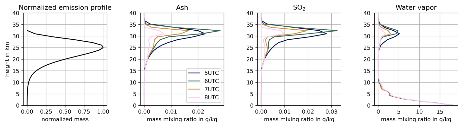
Figure A1 Emission profile (a) and vertical mass mixing ratio profiles 1 (blue), 2 (orange), 3 (green), and 4 (red) hours after the beginning of the first emission phase for (b) ash, (c) SO₃, and (d) water vapor.

Appendix B: Temperature and humidity in aerosol plume

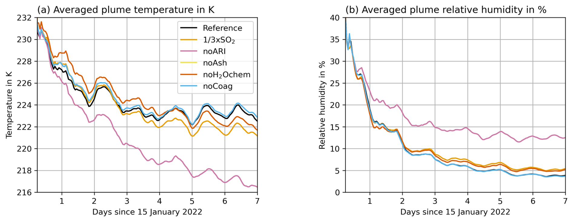
Figure B1 Aerosol-plume averaged (a) temperature in K and (b) specific humidity in % in all experiments that include the volcanic eruption to explain the difference in the water uptake.

Appendix C: Additional plots for SO₂ and sulfate comparisons

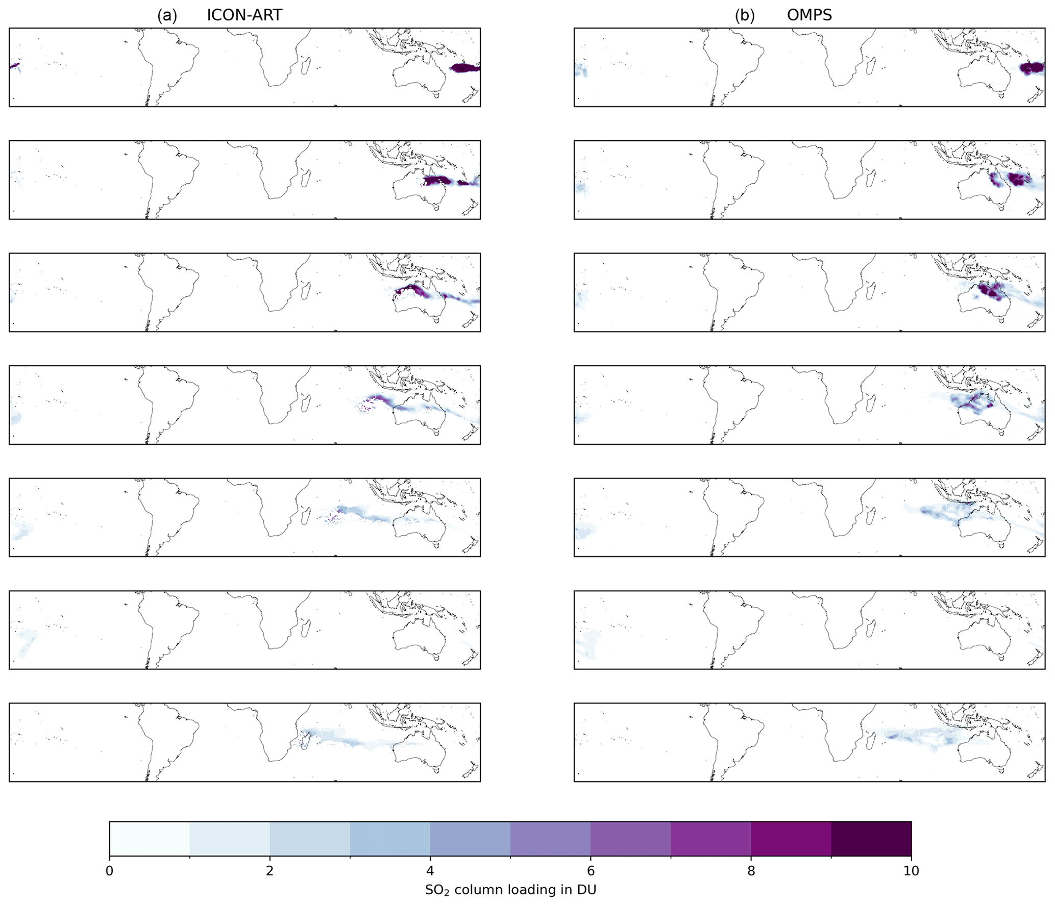
Figure C1 Comparison of the ICON-ART (a) and OMPS (b) SO₂ column loadings in DU for all detected overpasses. The rows from top to bottom refer to the following dates: 16 January, 02:00–04:00 UTC; 17 January, 02:00–05:00 UTC; 18 January, 01:00–06:00 UTC; 19 January, 01:00–08:00 UTC; 20 January, 01:00–09:00 UTC; 21 January, 00:00–02:00 UTC; and 21 January, 05:00–11:00 UTC.

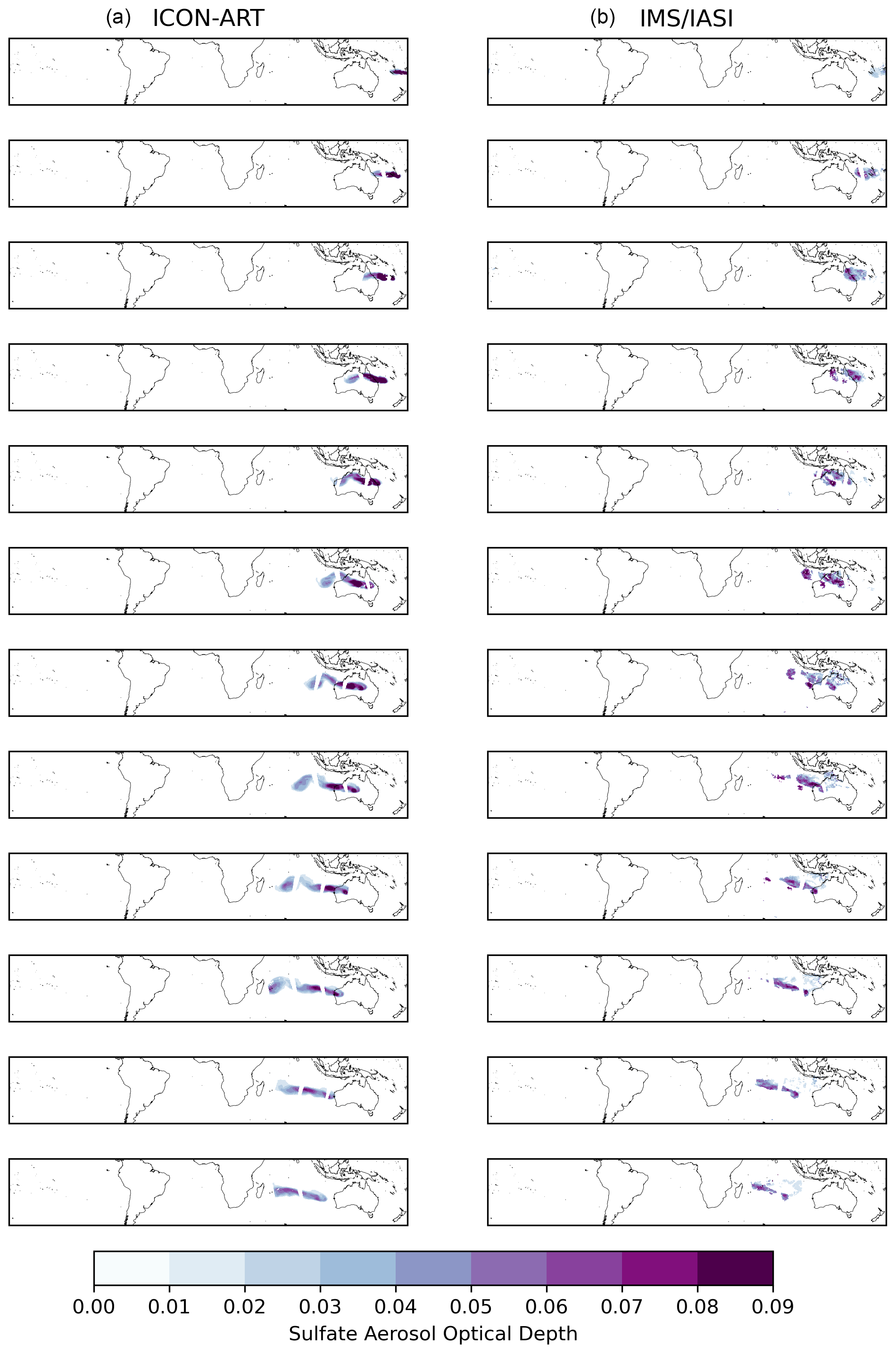
Figure C2 Comparison of the ICON-ART (a) and IMS/IASI (b) SAOD for all detected overpasses. The rows from top to bottom refer to the following dates: 15 January, 21:00 UTC; 16 January, 10:00–12:00 UTC; 16 January, 21:00–23:00 UTC; 17 January, 11:00–13:00 UTC; 17 January, 22:00 UTC–18 January 02:00 UTC; 18 January, 11:00–14:00 UTC; 19 January, 00:00–03:00 UTC; 19 January, 12:00–16:00 UTC; 20 January, 01:00–04:00 UTC; 20 January, 13:00–17:00 UTC; 21 January, 01:00–4:00 UTC; and 21 January, 15:00–17:00 UTC.

Appendix D: CALIPSO overpass

Figure D1 Same as Fig. 6 but for 16 January 2022 at 16:00 UTC.

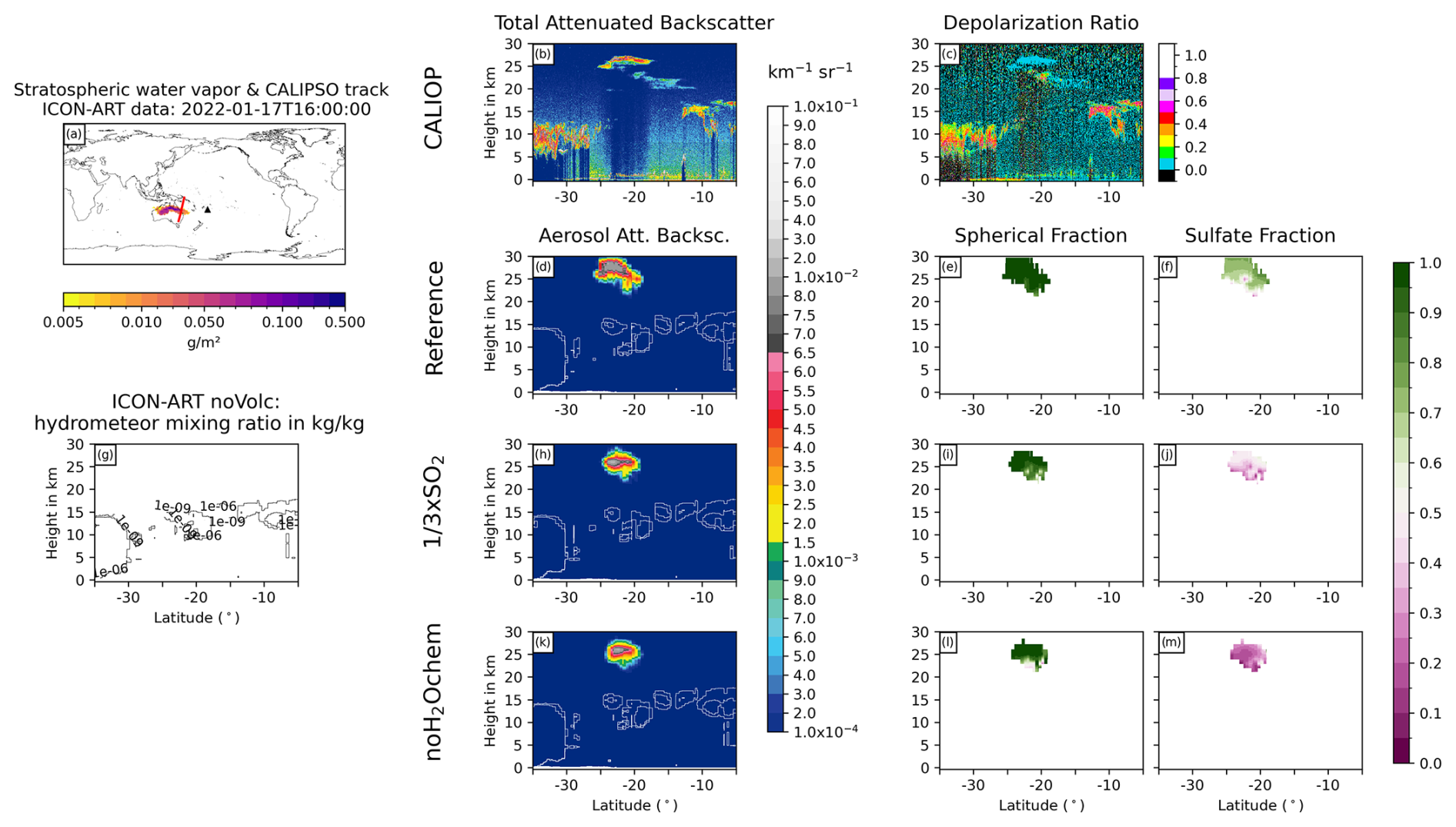
Figure D2 Same as Fig. 6 but for 17 January 2022 at 16:00 UTC.

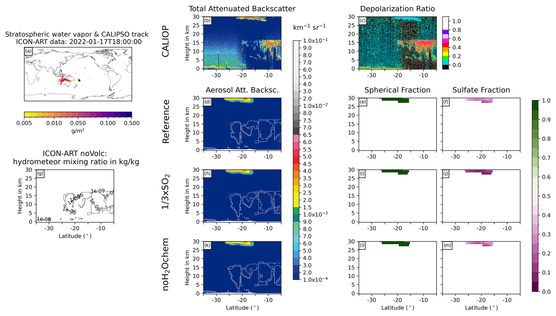
Figure D3 Same as Fig. 6 but for 17 January 2022 at 18:00 UTC.

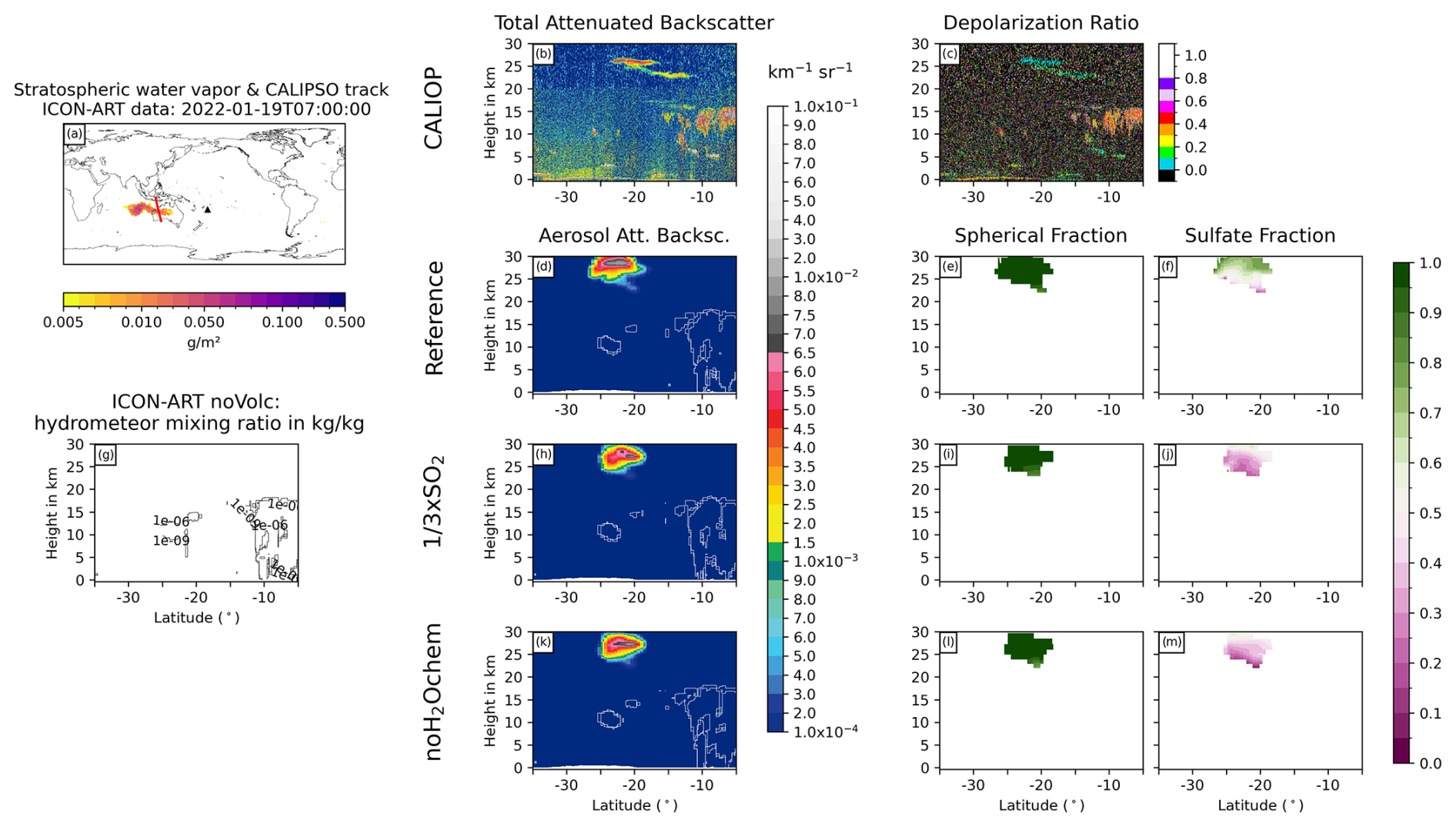
Figure D4 Same as Fig. 6 but for 19 January 2022 at 07:00 UTC.

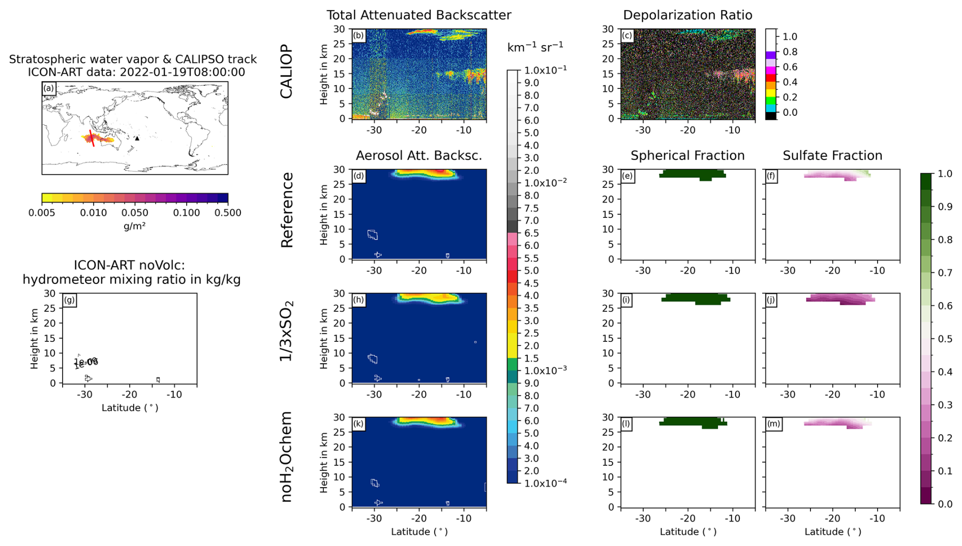
Figure D5 Same as Fig. 6 but for 19 January 2022 at 08:00 UTC.

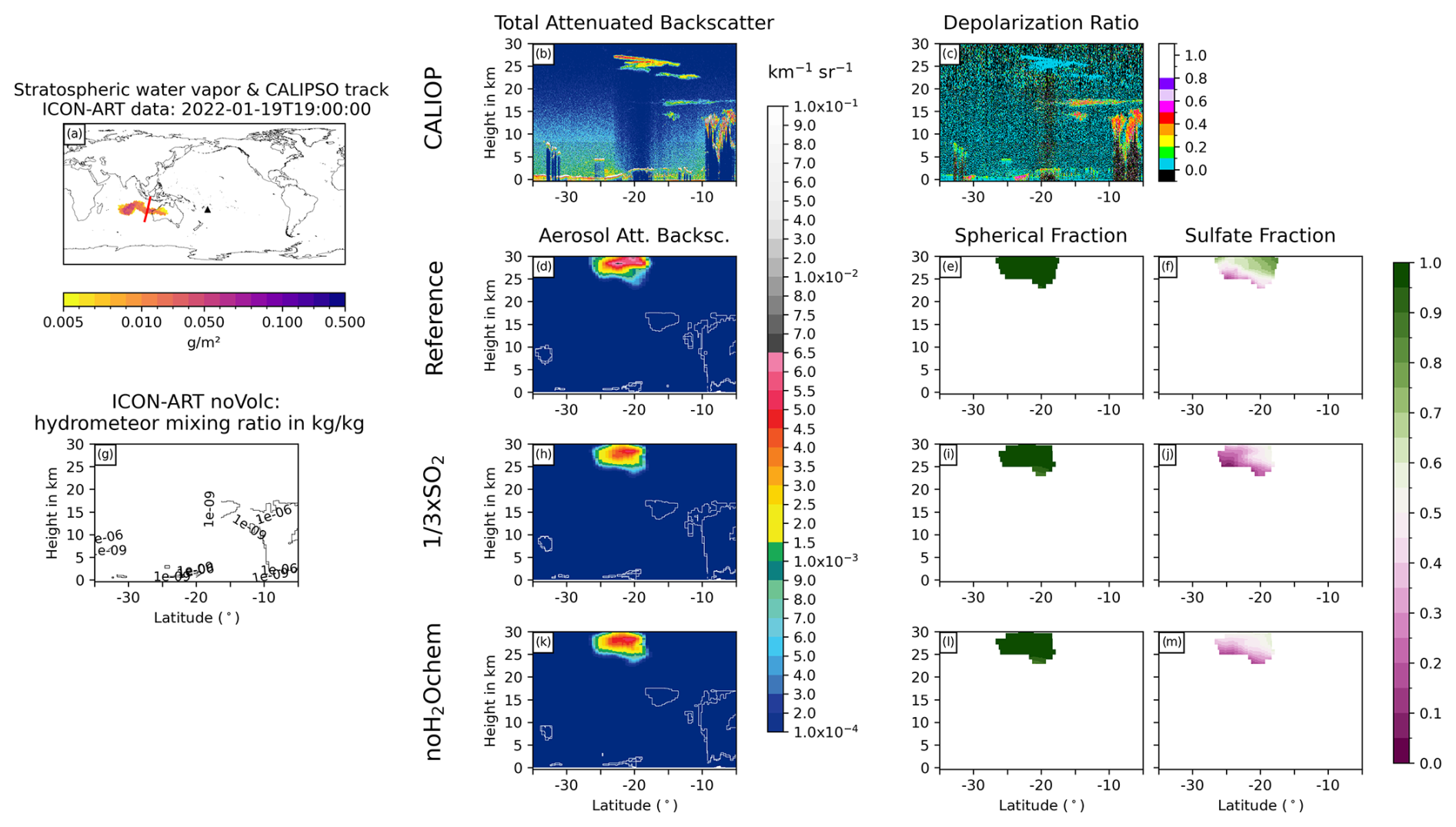
Figure D6 Same as Fig. 6 but for 19 January 2022 at 19:00 UTC.

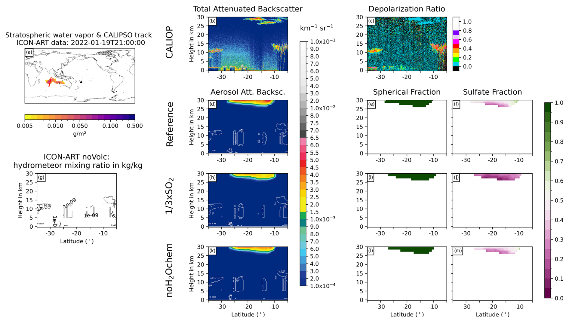
Figure D7 Same as Fig. 6 but for 19 January 2022 at 21:00 UTC.