Constraining elemental mercury air–sea exchange using long-term ground-based observations

Air–sea exchange of gaseous elemental mercury (Hg⁰) is a major component of the global mercury (Hg) biogeochemical cycle but remains poorly understood due to sparse in situ measurements. Here, we used long-term atmospheric Hg⁰ (${\mathrm{Hg}}_{\text{air}}^{\mathrm{0}}$) observations combined with air mass back trajectories at four ground-based monitoring sites to study Hg⁰ air–sea exchange. The trajectories showed that all four sites sample mainly marine air masses. At all sites, we observed a gradual increase in mean ${\mathrm{Hg}}_{\text{air}}^{\mathrm{0}}$ concentration with air mass recent residence time in the marine boundary layer (MBL), followed by a steady state. The pattern is consistent with the thin-film gas exchange model, which predicts net Hg⁰ emissions from the surface ocean until the ${\mathrm{Hg}}_{\text{air}}^{\mathrm{0}}$ concentration normalised by Henry's law constant matches the surface ocean dissolved Hg⁰ (${\mathrm{Hg}}_{\text{aq}}^{\mathrm{0}}$) concentration. This provides strong evidence that ocean Hg⁰ emissions directly influence ${\mathrm{Hg}}_{\text{air}}^{\mathrm{0}}$ concentrations at these sites. Using the observed relationship between ${\mathrm{Hg}}_{\text{air}}^{\mathrm{0}}$ concentrations and air mass recent MBL residence time, we estimated mean surface ocean ${\mathrm{Hg}}_{\text{aq}}^{\mathrm{0}}$ concentrations of 4–7 pg L⁻¹ for the North Atlantic and Arctic oceans (AA) and 4 pg L⁻¹ for the Southern, South Atlantic and south Indian oceans (SSI). Estimated ocean Hg⁰ emission fluxes ranged between 0.57–0.86 and 0.60–0.87 $\mathrm{ng}{\mathrm{m}}^{-\mathrm{2}}{\mathrm{h}}^{-\mathrm{1}}$ for the AA and SSI, respectively, with a global extrapolated mean flux of around 2270 t yr⁻¹ (1600–2900 t yr⁻¹). This study demonstrates the applicability of long-term, ground-based ${\mathrm{Hg}}_{\text{air}}^{\mathrm{0}}$ observations in constraining Hg⁰ air–sea exchange.

1 Introduction

Mercury (Hg), a ubiquitous element in the environment, has gained widespread attention due to its adverse effects on human health and ecosystems (AMAP/UN Environment, 2019; Budnik and Castelyn, 2019; Al-Sulaiti et al., 2022; Basu et al., 2023). While naturally occurring in the Earth's crust and released by natural processes, anthropogenic activities have dramatically increased the amount of Hg emitted into the environment (Sunderland and Mason, 2007; Amos et al., 2013; Lamborg et al., 2014; Zhang et al., 2014; Streets et al., 2017; Li et al., 2020; Sonke et al., 2023). Consequently, Hg has become a persistent global pollutant.

The elemental form of Hg (Hg⁰) is particularly important. Owing to its chemical inertness and low water solubility, once emitted, Hg⁰ stays in the atmosphere for several months to a year (Horowitz et al., 2017; Saiz-Lopez et al., 2018; Shah et al., 2021), allowing it to travel thousands of kilometres across the globe, impacting even remote areas (Travnikov, 2005; Durnford et al., 2010; Koenig et al., 2022). Although in the atmosphere Hg⁰ exists in low concentrations with no direct harmful effects (Holloway and Littlefield, 2011), a portion of the atmospheric Hg⁰ is gradually oxidised to more soluble divalent Hg compounds (Hg^II) that are readily deposited to surface reservoirs (Horowitz et al., 2017; Saiz-Lopez et al., 2018; Shah et al., 2021). In aquatic environments, some of this deposited Hg^II is converted to methylmercury (Lehnherr, 2014), a highly toxic compound that bioaccumulates and is biomagnified up the food chain (Lehnherr, 2014), posing serious health risks to humans through the consumption of seafood (Driscoll et al., 2013; Zillioux, 2015; AMAP/UN Environment, 2019; Al-Sulaiti et al., 2022).

The exchange of Hg⁰ between the atmosphere and the oceans plays a crucial role in the cycling of Hg in the environment. Atmospheric deposition, being the dominant source of Hg (Hg⁰, as well as Hg^II) entering the ocean (Horowitz et al., 2017; AMAP/UN Environment, 2019; Zhang et al., 2019, 2023; Jiskra et al., 2021; Shah et al., 2021), strongly influences the distribution of aqueous Hg (Strode et al., 2007; Kuss et al., 2011; Soerensen et al., 2014). On the other hand, most of the deposited Hg is eventually re-emitted back to the atmosphere, with ocean emissions constituting about one-third of the total annual Hg released to the atmosphere (Horowitz et al., 2017; AMAP/UN Environment, 2019; Zhang et al., 2019; Shah et al., 2021). Through this “multihop” mechanism (Hedgecock and Pirrone, 2004), where atmospheric Hg is deposited to the ocean and the ocean re-emits it back to the atmosphere (as Hg⁰), ocean emissions contribute to the long-range transport of Hg⁰ and extend the lifetime of Hg actively cycling in the environment (Strode et al., 2007; Amos et al., 2013). Conversely, a reduction in dissolved Hg^II to Hg⁰ in the water column and its subsequent evasion decreases the Hg^II reservoir available for conversion to methylmercury (Lehnherr, 2014). Evidently, accurately characterising Hg⁰ air–sea exchange is critical.

Our understanding of Hg⁰ air–sea exchange and cycling in the marine boundary layer (MBL) mainly derives from in situ measurements performed during ship-board sampling campaigns (e.g. Gårdfeldt et al., 2003; Andersson et al., 2007, 2008b, 2011; Kuss et al., 2011; Soerensen et al., 2013, 2014; Mason et al., 2017; Nerentorp Mastromonaco et al., 2017; Wang et al., 2017, 2019). These observations, comprised of simultaneous measurements of Hg⁰ in air (${\mathrm{Hg}}_{\text{air}}^{\mathrm{0}}$) and in surface seawater (${\mathrm{Hg}}_{\text{aq}}^{\mathrm{0}}$), along with variables such as sea surface temperature (SST) and wind speed, have been instrumental in discerning the spatio-temporal variability in Hg⁰ at the air–sea interface, estimating Hg⁰ air–sea exchange fluxes, as well as understanding the factors driving these processes. However, these measurements are sparse, covering only short periods (typically a few days to a few weeks), and are predominantly performed in the Northern Hemisphere. Chemical transport models can provide insights beyond the spatio-temporal limitations of in situ measurements, but they are also limited by the sparsity of direct measurements, such as for validating air–sea exchange parameterisations applied in the models (e.g. Zhang et al., 2019). As a result, many aspects of Hg⁰ dynamics at the air–sea interface remain poorly understood.

Some ground-based monitoring sites sample air masses with extended ocean exposure, offering a valuable opportunity to study Hg⁰ cycling at the air–sea interface. Moreover, many of these sites have continuous ${\mathrm{Hg}}_{\text{air}}^{\mathrm{0}}$ records spanning several years (e.g. Sprovieri et al., 2016). Despite their potential, their application for extensive analyses of Hg⁰ air–sea exchange remains underexplored, with studies primarily using them for model validation (e.g. Soerensen et al., 2010b) or for complementing ship-based measurements (e.g. Gårdfeldt et al., 2003; Sommar et al., 2010).

In this paper, we analyse ${\mathrm{Hg}}_{\text{air}}^{\mathrm{0}}$ observations from four ground-based monitoring sites to study Hg⁰ air–sea exchange. We use measurements from the longest continuous monitoring sites in the Northern Hemisphere (NH) and Southern Hemisphere (SH), Mace Head and Cape Point, respectively, as well as from the subtropical North Atlantic site Cabo Verde Observatory and the remote southern Indian Ocean site Amsterdam Island. The observations are combined with air mass back trajectories to gain insights into the sources and travel paths of air masses sampled at the sites. The results from this study will contribute towards an improved understanding of Hg⁰ air–sea exchange.

2 Data and methods

2.1 Observations

2.1.1 Site descriptions

We used observations from four monitoring sites, namely Mace Head, Cabo Verde Observatory, Cape Point and Amsterdam Island (Fig. 1). Below is a brief description of each site.

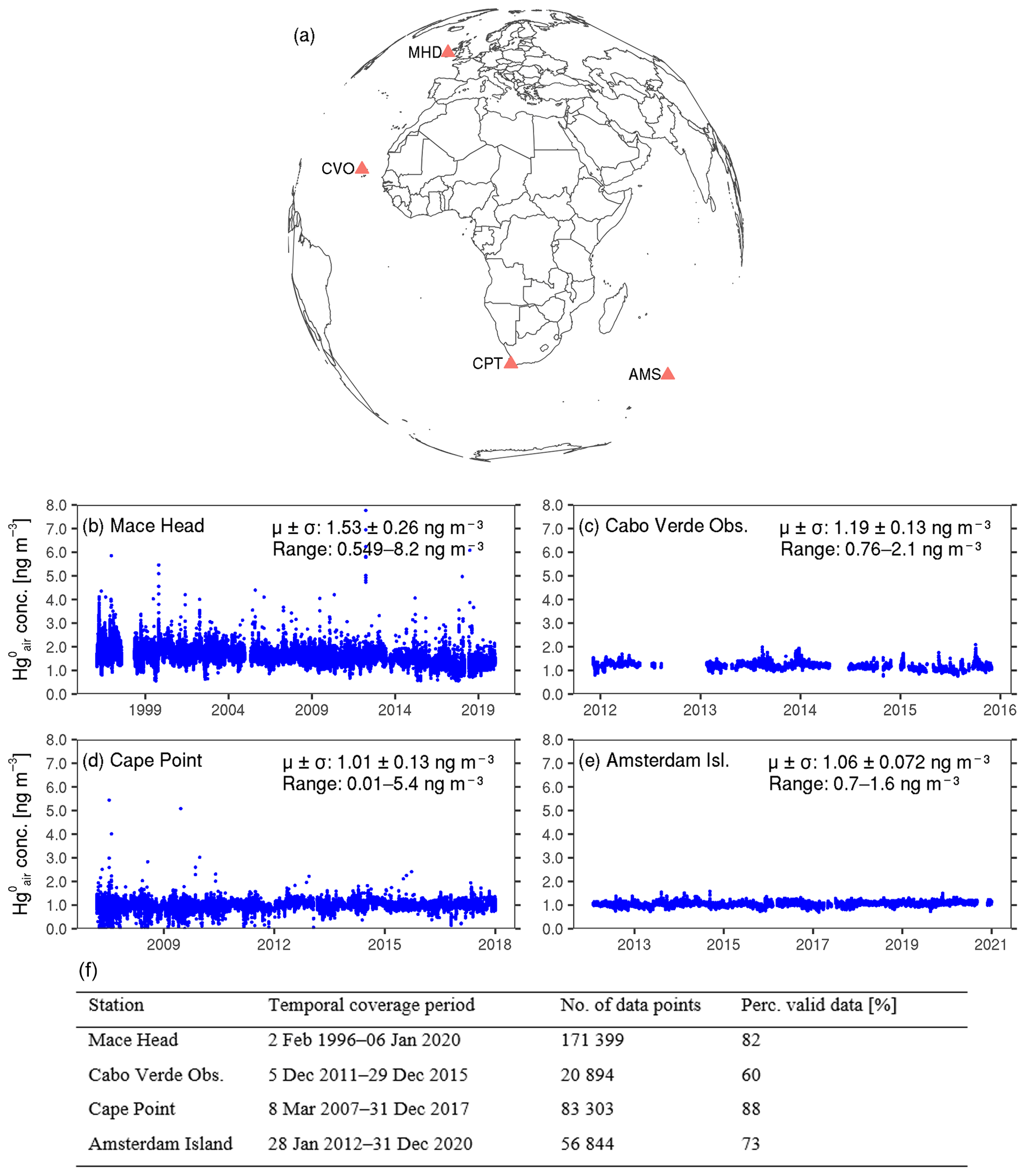
Figure 1 Overview of the ${\mathrm{Hg}}_{\text{air}}^{\mathrm{0}}$ data used in the study. (a) Map showing the locations of the four study sites: Mace Head (MHD), Cabo Verde Observatory (CVO), Cape Point (CPT) and Amsterdam Island (AMS). (b–e) Hourly mean ${\mathrm{Hg}}_{\text{air}}^{\mathrm{0}}$ concentrations at Mace Head, Cabo Verde Observatory, Cape Point and Amsterdam Island, respectively. The mean ±1 standard deviation and the range of the hourly observations are shown in each panel. Note that the extent of the x axis differs across the four sites. For better readability of the data, for where the y axis scales are adjusted to each site's data distribution, see Fig. S1 in the Supplement. (f) Summary of the hourly mean ${\mathrm{Hg}}_{\text{air}}^{\mathrm{0}}$ data coverage at the four sites, showing the temporal coverage of the observations used in the present study, the total number of hourly data points and the percentage of hourly time stamps over the coverage period with (valid or non-missing) data.

Mace Head

Mace Head (53°20^′ N, 9°54^′ W) is located in County Galway on the west coast of Ireland (Ebinghaus et al., 2011). It is exposed to the North Atlantic Ocean with a wide clean sector between 180 and 300° (Ebinghaus et al., 2011), ideally situated to study atmospheric composition under northern hemispheric background conditions but also under regionally polluted European continental conditions, when air masses originate from an easterly direction (Ebinghaus et al., 2011). On average, over 50 % of air masses that arrive at Mace Head are within the clean sector, having recently travelled thousands of kilometres across the North Atlantic Ocean (Ebinghaus et al., 2011). The climate at Mace Head is mild and moist (https://www.macehead.org, last access: June 2022), with an average air temperature of about 10 °C, generally high relative humidity (80 %–85 %) and an annual rainfall of approximately 1200 mm. Air sampling at the site is performed from two towers (10 and 22 m high) located 100 m from the shoreline and 50 m from the high-water mark. There are no industrial activities that could influence the measurements at Mace Head (Ebinghaus et al., 2011), with the nearest major urban area, Galway city, situated about 90 km east of the station (Ebinghaus et al., 2011). Mace Head is operated by the Atmospheric Science Research Group at the National University of Ireland, Galway (Kock et al., 2005), and is part of multiple international research networks, including the Global Mercury Observation System (GMOS) and the Global Atmosphere Watch (GAW) of the World Meteorological Organisation (WMO).

Cabo Verde Observatory

Cabo Verde Observatory (16°51^′ N, 24°52^′ W) lies on the northeast side of São Vicente (Read et al., 2017), one of ten islands in the Cabo Verde archipelago in the North Atlantic Ocean (Read et al., 2017). The site is characterised by a warm and dry climate, with a mean annual air temperature of 24 ± 2 °C and annual rainfall below 200 mm, most of which occurs in the rainy season of July–November (Read et al., 2017). The observatory receives mostly (about 95 % of the time) air masses from the northeasterly trade winds, which have typically travelled for 5 d over the ocean (Read et al., 2017), providing the opportunity to study clean marine air (Carpenter et al., 2010; Read et al., 2017). Air sampling at Cabo Verde Observatory is performed 50 m from the coastline at 10 m above sea level (Carpenter et al., 2010). The observatory is operated as a multilateral project between the United Kingdom, Germany and the Republic of Cabo Verde (Read et al., 2017) and is also part of both the GMOS and WMO-GAW network of sites (Carpenter et al., 2010; Sprovieri et al., 2016; Read et al., 2017).

Cape Point

Cape Point (34°21^′ S, 18°29^′ E) is located on the southern tip of the Cape Peninsula, about 60 km south of Cape Town, South Africa (Martin et al., 2017). It is situated within the Cape Point National Park, on a coastal cliff 230 m above sea level (Brunke et al., 2004; Martin et al., 2017). The site has a Mediterranean-type climate, characterised by moderate temperatures, dry summers and increased precipitation during winter (Brunke et al., 2004). The prevailing wind direction at Cape Point is from the southeast to southwest, and thus most air masses advected to the site are clean marine air from the Southern Ocean (Brunke et al., 2004). On average, over 50 % of the air masses reaching Cape Point originate from this clean oceanic sector, having recently travelled thousands of kilometres across the southern oceanic regions (Labuschagne et al., 2018). Nevertheless, the site occasionally experiences air masses from the north to northeast, mainly in winter, that are influenced by anthropogenic emissions from the greater Cape Town area and/or by other continental sources (Brunke et al., 2010). Cape Point is operated by the South African Weather Service (SAWS) and is also part of the GMOS and WMO-GAW networks (Martin et al., 2017; Slemr et al., 2020).

Amsterdam Island

Amsterdam Island (37°48^′ S, 77°34^′ E) is a small subtropical island (55 km²) in the southern Indian Ocean, located about 3400 and 5000 km downwind of Madagascar and South Africa, respectively (Angot et al., 2014; Slemr et al., 2015, 2020; Li et al., 2023; Magand et al., 2023; Tassone et al., 2023). The atmospheric monitoring station is situated at Pointe Bénédicte at the northwest end of the island at an altitude of 70 m above sea level (Angot et al., 2014; Magand et al., 2023). Air sampling and monitoring at the Pointe Bénédicte station are performed from different heights depending on the pollutant studied, with atmospheric Hg being sampled at 6 m above ground level. The site has an oceanic climate with mild temperatures (ranging between 11 and 17 °C over the year), high relative humidity (65 % to 85 %), and the frequent presence of clouds and abundant rainfall (total annual average between ∼800 and ∼1300 mm from the last decades) (Miller et al., 1993; Angot et al., 2014; Tassone et al., 2023). The dominant surface wind direction at Amsterdam Island is westerly and northwesterly, and wind speeds are comparatively high throughout the year (with an annual average of 7.6 m s⁻¹; Miller et al., 1993), peaking in austral winter (Baboukas et al., 2004; Li et al., 2023). The island is largely free of human disturbance. The only possible, but very rare, local source of pollution may emanate from the 20–40 scientific research and technical crew in Martin-de-Viviès life base 2 km downwind of the Pointe Bénédicte station. Amsterdam Island is run under the administration of Terres Australes et Antarctiques Françaises (TAAF), the French Southern and Antarctic Lands, and is scientifically operated by the French Polar Institute (IPEV) research programmes all year round. The monitoring station is part of the French national monitoring system, the Integrated Carbon Observation System, ICOS-France Atmosphère, for the long-term observation of greenhouse gases (El Yazidi et al., 2018; Magand et al., 2023). As with Mace Head, Cabo Verde Observatory and Cape Point, the Pointe Bénédicte station in Amsterdam Island is part of both the GMOS network and is also labelled as a WMO-GAW site (Angot et al., 2014; Slemr et al., 2015, 2020; Magand et al., 2023).

2.1.2 Atmospheric Hg measurements

Atmospheric Hg has been measured since September 1995, December 2011, March 2007 and January 2012 at Mace Head, Cabo Verde Observatory, Cape Point and Amsterdam Island, respectively, using Tekran 2537 A/B model analysers (Tekran Inc., Toronto, Canada; Ebinghaus et al., 2002; Read et al., 2017; Slemr et al., 2020; Magand et al., 2023). The analysers are based on Hg enrichment on a gold cartridge, followed by thermal desorption and detection by cold vapour atomic fluorescence spectroscopy (CVAFS) at 253.7 nm (Fitzgerald and Gill, 1979; Bloom and Fitzgerald, 1988). The analysers use two gold cartridges, switching between the cartridges to allow for alternating sampling and desorption, resulting in continuous sampling of the incoming air (Ebinghaus et al., 2011; Martin et al., 2017; Slemr et al., 2020; Magand et al., 2023). Concentrations are expressed in nanograms per cubic metre at standard temperature and pressure (STP) conditions (273.15 K, 1013.25 hPa) with an instrumental detection limit close to 0.1 ng m⁻³ and an ${\mathrm{Hg}}_{\text{air}}^{\mathrm{0}}$ average uncertainty value of about 10 % (Slemr et al., 2015).

The instruments are automatically calibrated every 25 h at Mace Head and Cape Point, every 72 h at Cabo Verde Observatory, and every 69 h at Amsterdam Island using internal permeation sources (Ebinghaus et al., 2011; Read et al., 2017; Slemr et al., 2020; Magand et al., 2023). The permeation sources are in turn checked (annually at Cabo Verde Observatory and Cape Point, bi-annually at Mace Head, and quarterly at Amsterdam Island) by manual injections of saturated Hg vapour from a temperature-controlled vessel adapted following Dumarey et al. (1985) procedures (Ebinghaus et al., 2011; Slemr et al., 2020; Magand et al., 2023). To ensure comparable results, the Tekran analysers at all four sites are operated and calibrated under GMOS standard operating procedures (SOPs; Sprovieri et al., 2016; Martin et al., 2017; Read et al., 2017; Slemr et al., 2020). The sampling procedure, quality assurance and quality control measures in operation at the sites are detailed in several references (e.g. Ebinghaus et al., 2011; Angot et al., 2014; Sprovieri et al., 2016; Slemr et al., 2020; Magand et al., 2023).

Several studies referenced here, including some of which use the same atmospheric Hg observations as those in the present study (i.e. from the same monitoring sites), denote Tekran 2537A/B measurements as total gaseous mercury (TGM; $\text{TGM}={\mathrm{Hg}}_{\text{air}}^{\mathrm{0}}$ + gaseous oxidised mercury, ${\mathrm{Hg}}_{\text{air}}^{\text{II}}$) (e.g. Gårdfeldt et al., 2003; Temme et al., 2003; Kock et al., 2005; Xia et al., 2010; Andersson et al., 2011; Ebinghaus et al., 2011; Read et al., 2017). However, at all four sites studied here, it has been suggested that the measurements are most likely of ${\mathrm{Hg}}_{\text{air}}^{\mathrm{0}}$ rather than TGM, as ${\mathrm{Hg}}_{\text{air}}^{\text{II}}$ is easily lost to sea-salt deposits in the inlet tubing and filters of the instrument (Weigelt et al., 2015; Read et al., 2017; Slemr et al., 2020). In Amsterdam Island, between 2012 and 2015 atmospheric mercury species were measured using a Tekran Hg speciation unit (Tekran 1130/1135 models), ensuring that only ${\mathrm{Hg}}_{\text{air}}^{\mathrm{0}}$ is sampled and analysed with the associated Tekran 2537A/B model. Since the deinstallation of the speciation unit at the site in 2015, the Tekran 2537A/B instrument has been deployed with a specific setup using two 0.45 µm polyethersulfone cation-exchange membranes (PES-CEMs, 0.45 µm, 47 mm, Merck Millipore^®) installed at the inlet of the heated line, preventing the introduction of oxidised species and ensuring that only ${\mathrm{Hg}}_{\text{air}}^{\mathrm{0}}$ is measured (Magand et al., 2023). Furthermore, TGM typically comprises mostly (>98 %) ${\mathrm{Hg}}_{\text{air}}^{\mathrm{0}}$ (e.g. Soerensen et al., 2010a; Cheng et al., 2014; Yin et al., 2018; Wang et al., 2019). Therefore, we regard the Tekran 2537A/B measurements at the four sites as ${\mathrm{Hg}}_{\text{air}}^{\mathrm{0}}$ and make no distinction between TGM and ${\mathrm{Hg}}_{\text{air}}^{\mathrm{0}}$, referring to the measurements as ${\mathrm{Hg}}_{\text{air}}^{\mathrm{0}}$, when referencing the above-mentioned studies.

The record of hourly mean ${\mathrm{Hg}}_{\text{air}}^{\mathrm{0}}$ observations from the four sites used in this study is presented in Fig. 1. Throughout this paper, the data were analysed and are presented in their local time.

2.1.3 ²²²Rn measurements from Cape Point

Since 1999, atmospheric radon (²²²Rn) has been continuously measured at Cape Point using a two-flow-loop, dual-filter detector designed by the Australian Nuclear Science and Technology Organisation (ANSTO) and partially constructed locally (Brunke et al., 2004; Botha et al., 2018). The instrument operates by passing ambient air through a particulate filter into a large chamber, where the ²²²Rn gas decays (Brunke et al., 2004). A second filter collects the ²²²Rn decay products, which are detected by means of a screen coated with the scintillator material zinc sulfide and viewed by a photomultiplier (Brunke et al., 2004). The count rate is proportional to the ambient ²²²Rn concentration (Brunke et al., 2004). The detector at Cape Point has been continuously developed (Brunke et al., 2004; Botha et al., 2018). In 2011, an upgraded version of the instrument was installed, incorporating system design improvements such as an automated calibration system and a delay volume, increasing the accuracy and reliability of the measurements at the site (Botha et al., 2018).

As described in detail in Botha et al. (2018), the radon detector's sample inlet is located 30 m above ground level and ²²²Rn is measured at a resolution of 30 min and further processed to an average 1 h temporal resolution. The detector is calibrated monthly by introducing a known concentration of ²²²Rn from a calibration source (²²⁶Ra source with ²²²Rn production rate of 2.94 Bq min⁻¹) acquired from Pylon Electronics, Inc., Canada (Brunke et al., 2004). The instrument has a lower limit of detection of 25 ± 8 mBq m⁻³, and the hourly measurements have an uncertainty of around 15 % at 100 mBq m⁻³ and 9 % at 1000 mBq m⁻³ (Botha et al., 2018).

In this work, we use hourly ²²²Rn data corresponding to the period of the Cape Point Hg⁰ dataset (i.e. the period 8 March 2007–31 December 2017).

2.2 Air mass back trajectories

We applied the Hybrid Single-Particle Lagrangian Integrated Trajectory (HYSPLIT) model (Stein et al., 2015) to trace air masses arriving at the monitoring sites. For each station and hour of the day, we calculated a 144 h (6 d) air mass back trajectory starting at 50 m above model ground level, using the National Centers for Environmental Prediction/National Center for Atmospheric Research (NCEP/NCAR) reanalysis data with a 2.5° spatial and a 6-hourly temporal resolution (Kalnay et al., 1996) for model input. Each of the 144 segments of every trajectory was then assigned to one of two categories based on the underlying surface over which the segment is passing:

• marine (or oceanic): segments passing over an area where the bathymetric elevation is 0 m or below;

• terrestrial (or land): segments passing over an area where the bathymetric elevation is above 0 m.

The bathymetry information was obtained from the GEneral Bathymetric Chart of the Oceans Grid (GEBCO_GRID), with a 15 arcsec spatial resolution (GEBCO Compilation Group, 2020). The segments were further classified into one of two categories, according to their height in the atmosphere:

• boundary layer: segments at or below the height of the planetary boundary layer (PBL);

• free tropospheric: segments above the height of the PBL.

For this step, we used PBL height data from the ERA5 re-analysis product of the European Centre for Medium-Range Weather Forecasts (ECMWF; Hersbach et al., 2020), with a temporal resolution of 1 h and a spatial resolution of 0.25°×0.25°. Therefore, each of the 144 segments of every trajectory was assigned to one of four categories: marine boundary layer (MBL), free troposphere over the ocean (FT_ocean), continental planetary boundary layer (CPBL) or free troposphere over land (FT_terrestrial; see Fig. S2).

3 Results and discussion

3.1 Overview of ${\mathrm{Hg}}_{\text{air}}^{\mathrm{0}}$ observations at Mace Head, Cabo Verde Observatory, Cape Point and Amsterdam Island

The record of hourly averaged ${\mathrm{Hg}}_{\text{air}}^{\mathrm{0}}$ measurements at the four sites is shown in Fig. 1. Over the analysis periods, the mean ${\mathrm{Hg}}_{\text{air}}^{\mathrm{0}}$ concentration was 1.53 ± 0.26, 1.19 ± 0.13, 1.01 ± 0.13 and 1.06 ± 0.07 ng m⁻³ (mean ±1 standard deviation) at Mace Head, Cabo Verde Observatory, Cape Point and Amsterdam Island, respectively. The higher mean concentration at Mace Head and, to a lesser extent, Cabo Verde Observatory compared to Cape Point and Amsterdam Island is consistent with previous studies that have reported higher ${\mathrm{Hg}}_{\text{air}}^{\mathrm{0}}$ levels in the NH than in the SH (e.g. Temme et al., 2003; Soerensen et al., 2010a, 2014; Sprovieri et al., 2010, 2016; Xia et al., 2010). The inter-hemispheric gradient in ${\mathrm{Hg}}_{\text{air}}^{\mathrm{0}}$ concentrations has been widely discussed in the literature and is largely attributed to the bulk burden of anthropogenic Hg emissions occurring in the NH (Temme et al., 2003; Sprovieri et al., 2010, 2016; Streets et al., 2017; AMAP/UN Environment, 2019).

Figure 2 shows the seasonal variability in monthly mean ${\mathrm{Hg}}_{\text{air}}^{\mathrm{0}}$ concentrations across the four sites. At Mace Head, ${\mathrm{Hg}}_{\text{air}}^{\mathrm{0}}$ levels are slightly but significantly higher in winter (December to May, 1.57 ± 0.27 ng m⁻³, n=84 228) than in summer (June to November, averaging 1.48 ± 0.25 ng m⁻³, n=87 171) ($p<\mathrm{2.2}\times {\mathrm{10}}^{-\mathrm{16}}$, Mann–Whitney U test). As with Mace Head, concentrations at Cabo Verde Observatory are slightly but significantly higher around winter (December–May, 1.22 ± 0.12, n=11 296) compared to summer (June–November, 1.16 ± 0.12, n=9598) ($p<\mathrm{2.2}\times {\mathrm{10}}^{-\mathrm{16}}$, Mann–Whitney U test). A similar seasonal pattern has been observed at other ground-based monitoring stations (e.g. Kock et al., 2005; Lan et al., 2012; Sprovieri et al., 2016; Jiskra et al., 2018) as well during ship-board sampling campaigns (e.g. Soerensen et al., 2010a) in the NH. Several explanations have been proposed for the northern hemispheric ${\mathrm{Hg}}_{\text{air}}^{\mathrm{0}}$ seasonality, including increased anthropogenic emissions from fossil-fuel combustion for heating in winter (Ebinghaus et al., 2002; Lan et al., 2012), higher ocean Hg⁰ emissions from the North Atlantic Ocean in winter (Soerensen et al., 2010b) and more recently increased vegetation Hg⁰ uptake in summer (Jiskra et al., 2018; Feinberg et al., 2022).

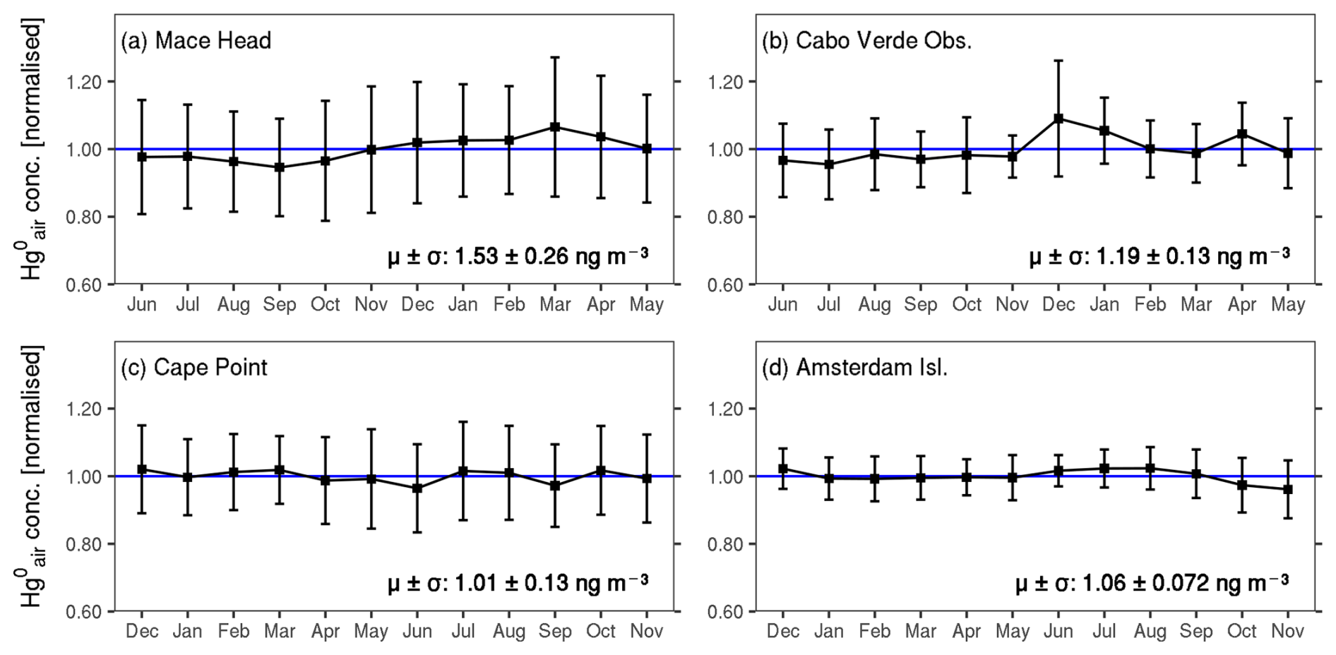
Figure 2 Normalised monthly mean ${\mathrm{Hg}}_{\text{air}}^{\mathrm{0}}$ concentrations at the four sites. The mean ±1 standard deviation of the hourly observations is shown in each panel. The bars show 1 standard deviation of the monthly means. The horizontal blue line represents the normalised mean value (i.e. 1 ng m⁻³). The months are ordered starting in June for Mace Head and Cabo Verde Observatory and in December for Cape Point and Amsterdam Island such that the plots consistently start in summer and end in spring (of the respective hemisphere).

Amsterdam Island shows slightly but significantly higher ${\mathrm{Hg}}_{\text{air}}^{\mathrm{0}}$ concentrations around winter (June–September, 1.07 ± 0.06, n=18 697) ($p<\mathrm{2.2}\times {\mathrm{10}}^{-\mathrm{16}}$, Mann–Whitney U test). Angot et al. (2014) as well as Slemr et al. (2020), who previously reported the same seasonality for the site, attributed it to long-range transport of polluted air masses from southern Africa between July and September, which coincides with the biomass-burning season in the region. Nevertheless, the observed winter peak at Amsterdam Island (in this study) corresponds to only a ∼1 % increase from the site's overall mean concentration. Similarly, at Mace Head as well as Cabo Verde Observatory, the winter maximum (summer minimum), though significantly higher (lower) than the overall mean concentration ($p<\mathrm{2.2}\times {\mathrm{10}}^{-\mathrm{16}}$, Mann–Whitney U test), represents only a ∼3 % change from the overall mean. No clear seasonality is detected at Cape Point.

The diurnal variability in ${\mathrm{Hg}}_{\text{air}}^{\mathrm{0}}$ at the four sites is quite weak as well, with daily mean minimum and maximum values reflecting just a ∼2 % change from the overall mean concentration (Fig. 3). The diurnal patterns also exhibit little seasonal variation (Fig. S3). Non-existent or non-significant ${\mathrm{Hg}}_{\text{air}}^{\mathrm{0}}$ diurnal variations in the marine boundary layer (MBL) have also been reported in other studies (e.g. Soerensen et al., 2010a; Wang et al., 2017, 2019).

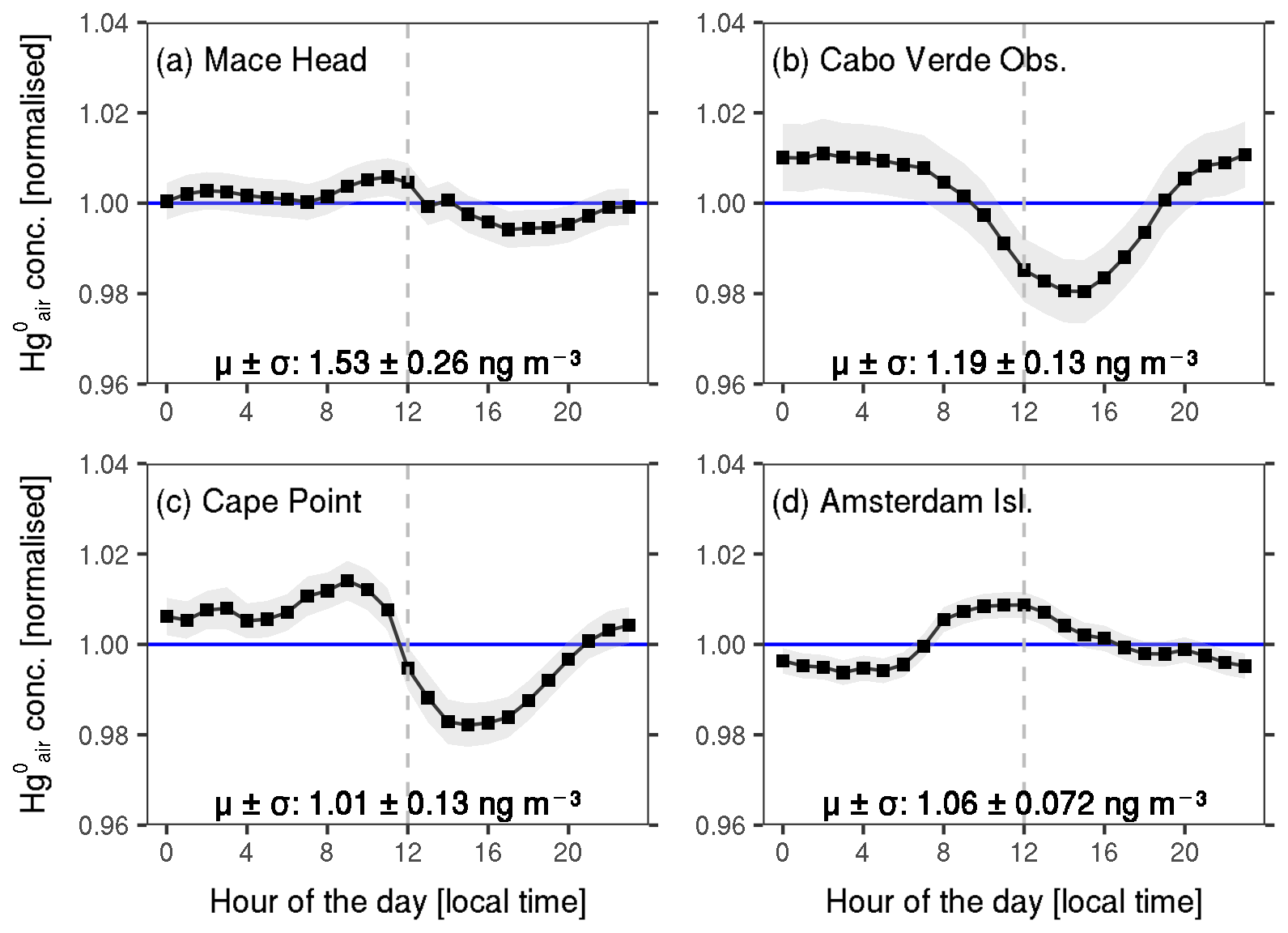
Figure 3 Normalised mean ${\mathrm{Hg}}_{\text{air}}^{\mathrm{0}}$ diurnal variation at (a) Mace Head, (b) Cabo Verde Observatory, (c) Cape Point and (d) Amsterdam Island. The mean ± the standard deviation of the hourly observations is shown for each site. The shaded area shows the mean ±2 times the standard error. The horizontal line represents the normalised mean value (i.e.  1 ng m⁻³), and the dashed vertical line is plotted along 12:00 LT.

3.2 ${\mathrm{Hg}}_{\text{air}}^{\mathrm{0}}$ in the MBL

A major goal of this work was to understand the dynamics of ${\mathrm{Hg}}_{\text{air}}^{\mathrm{0}}$ in the MBL, especially given the weak seasonal and diurnal variability in concentrations observed at our ground-based study sites. Previous research has highlighted Hg⁰ air–sea exchange as one of the key processes influencing ${\mathrm{Hg}}_{\text{air}}^{\mathrm{0}}$ concentrations in the MBL (e.g. Wängberg et al., 2001; Laurier et al., 2003; Soerensen et al., 2010a, b; Carbone et al., 2016; Wang et al., 2017). In turn, Hg⁰ air–sea exchange is suggested to be driven by two main factors: (i) the Hg⁰ concentration gradient at the air–sea interface and (ii) wind speed and solar radiation (e.g. Gårdfeldt et al., 2003; Wängberg et al., 2001; Laurier et al., 2003; Soerensen et al., 2010a, b; 2013; Kuss et al., 2011; Wang et al., 2017). Many studies show that ocean surface waters are primarily supersaturated in ${\mathrm{Hg}}_{\text{aq}}^{\mathrm{0}}$ relative to the overlaying air (e.g. Wängberg et al., 2001; Gårdfeldt et al., 2003; Andersson et al., 2011; Mason et al., 2017; Wang et al., 2017, 2019), creating conducive conditions for net ocean Hg⁰ emission to the atmosphere. In fact, recent estimates place ocean Hg⁰ evasion as the largest single net flux of Hg⁰ to the atmosphere, in the range of 2800–4000 Hg⁰ t yr⁻¹ (Horowitz et al., 2017; AMAP/UN Environment, 2019; Outridge et al., 2018; Shah et al., 2021; Zhang et al., 2023). Regarding wind speed and solar radiation, both variables generally exhibit pronounced seasonal and diurnal variability. Considering these factors, it would be expected that ${\mathrm{Hg}}_{\text{air}}^{\mathrm{0}}$ concentrations in the MBL also show pronounced seasonal and diurnal variability, but this is not the case.

While the four sites largely sample clean marine air, they are also occasionally affected by terrestrial sources and processes (e.g. Ebinghaus et al., 2002; Brunke et al., 2004; Slemr et al., 2013, 2020; Angot et al., 2014; Read et al., 2017; Bieser et al., 2020), albeit to varying degrees. As air masses from both the marine and terrestrial environment are sampled at the sites, this can obscure the link between observed ${\mathrm{Hg}}_{\text{air}}^{\mathrm{0}}$ concentrations and the oceanic Hg⁰ evasion signal. To distinguish between MBL conditions and terrestrial influences, we used the HYSPLIT back trajectories. We classified each hourly ${\mathrm{Hg}}_{\text{air}}^{\mathrm{0}}$ observation at the sites into one of three categories: MBL-influenced (MBL_i), terrestrial-influenced (Terr_i) and mixed (Mixed). MBL_i was assigned to observations where 90 % or more of the (144) back trajectory segments were classified as MBL, Terr_i to those where 90 % or more of the segments were classified as CPBL, and mixed was assigned to those where neither of the first two criteria is met (see Sect. 2.2 for the distinction between MBL- and CPBL-assigned trajectory segments). To validate the classification method, we (also) applied it to ²²²Rn observations from Cape Point. Considering that ²²²Rn emission by the ocean is negligible (at a rate 2 to 3 orders of magnitude lower than the terrestrial flux; Schery and Huang, 2004) and that ²²²Rn's terrestrial source is unaffected by human activity, its consistent emission over land makes it an excellent tracer for identifying air masses of terrestrial origin over the ocean or within the troposphere for 2–3 weeks (Brunke et al., 2010; Chambers et al., 2018). The ²²²Rn results, presented in Fig. S4, show generally higher ²²²Rn values for the Terr_i data compared to the MBL_i data, with a significantly larger mean concentration for the Terr_i data (3426 mBq m⁻³, n=56) compared to the MBL_i data (450 mBq m⁻³, n=30 470) ($p<\mathrm{2.2}\times {\mathrm{10}}^{-\mathrm{16}}$, Mann–Whitney U test). While ²²²Rn measurements are also available at Amsterdam Island, we did not perform the above analysis for the site, as we do not expect a strong terrestrial ²²²Rn signal due to the remoteness of the site (which is surrounded by over 3000 km of ocean) as well as the small size of the island.

Figures S5 and S6 show the seasonal and diurnal variations, respectively, for the MBL_i, Terr_i and Mixed ${\mathrm{Hg}}_{\text{air}}^{\mathrm{0}}$ datasets, along with the full observations (All data) at the four sites. The summary statistics for the groups are provided in Table S1 in the Supplement. In summary, the results show that the ${\mathrm{Hg}}_{\text{air}}^{\mathrm{0}}$ observations at the sites are largely associated with air masses strongly influenced by the MBL, with little to no contribution from air masses influenced by terrestrial surfaces. The results also show little difference between the ${\mathrm{Hg}}_{\text{air}}^{\mathrm{0}}$ temporal distributions (i.e. the seasonal and diurnal variations) of the full observations and the MBL_i (as well as the Mixed) data. This suggests that the weak seasonal and diurnal variations observed at the sites represent the actual MBL conditions and are not an artefact of sampling air masses from different environments.

In a recent publication, Koenig et al. (2023) analysed ${\mathrm{Hg}}_{\text{air}}^{\mathrm{0}}$ observations at Maïdo Observatory, a high-altitude station (2160 m above sea level) located on La Réunion Island in the southern tropical Indian Ocean (21°4^′ S, 55°48^′ E). The study derived a mean lower-free-troposphere (LFT) ${\mathrm{Hg}}_{\text{air}}^{\mathrm{0}}$ concentration of ∼0.73 ng m⁻³. Assuming that this value is also representative of the LFT over Cape Point and Amsterdam Island (located about 3900 and 2900 km from Maïdo observatory, respectively), the mean MBL (i.e. MBL_i) ${\mathrm{Hg}}_{\text{air}}^{\mathrm{0}}$ concentrations extracted at Cape Point and Amsterdam Island (1.01 ± 0.12 and 1.06 ± 0.07 ng m⁻³, respectively; Table S1) are both about 30 % larger than the LFT value from Koenig et al. (2023). In the NH, using aircraft data, Weigelt et al. (2016) reported an LFT ${\mathrm{Hg}}_{\text{air}}^{\mathrm{0}}$ concentration of about 1.3 ng m⁻³ over central Europe, which is about 15 % lower than the mean MBL concentration at Mace Head (1.53 ± 0.24 ng m⁻³). These higher MBL concentrations relative to LFT concentrations suggest net ocean Hg⁰ emissions into the MBL.

A question remains regarding the weak seasonal and diurnal variations in ${\mathrm{Hg}}_{\text{air}}^{\mathrm{0}}$ concentrations in the MBL. Another recent publication, Lamborg et al. (2021), has proposed that dark reduction, rather than photoreduction, as previously believed, is responsible for most of the ${\mathrm{Hg}}_{\text{aq}}^{\mathrm{0}}$ produced in the ocean and subsequently escaping to the atmosphere. Since dark reduction is less directly impacted by climatic conditions than photoreduction, this would imply constant (i.e. even under low solar radiation) ${\mathrm{Hg}}_{\text{aq}}^{\mathrm{0}}$ supply to the surface ocean. This would have two implications for Hg⁰ cycling in the air–sea interface. One, it would explain the weak temporal ${\mathrm{Hg}}_{\text{air}}^{\mathrm{0}}$ variability in the MBL, as dark reduction would provide a relatively constant pool of ${\mathrm{Hg}}_{\text{aq}}^{\mathrm{0}}$ to the surface ocean throughout the day and seasons. Secondly, and related to the first point, it would imply that the ocean is constantly emitting Hg⁰ to the atmosphere.

With these considerations, we sought to investigate the influence of air mass recent residence time in the MBL on observed ${\mathrm{Hg}}_{\text{air}}^{\mathrm{0}}$ concentrations. We hypothesise that an air mass entering the MBL from the LFT carries a signature ${\mathrm{Hg}}_{\text{air}}^{\mathrm{0}}$ concentration of this environment. As it travels within the MBL, there is exchange of Hg⁰ between the air mass and the surface ocean. Because the ocean surface layer is typically supersaturated in Hg⁰ relative to the atmosphere, there is net Hg⁰ emission to the atmosphere and consequently a gradual increase in the Hg⁰ concentration of the air mass over time. Therefore, air masses which have recently spent a long time in the MBL would generally have higher ${\mathrm{Hg}}_{\text{air}}^{\mathrm{0}}$ levels than those which have recently spent more time in the LFT. The results of the investigation are presented in the next section.

3.3 Relationship between observed ${\mathrm{Hg}}_{\text{air}}^{\mathrm{0}}$ concentrations and air mass residence time in the MBL

To test our hypothesis, we used the back trajectories to study the ${\mathrm{Hg}}_{\text{air}}^{\mathrm{0}}$ observations in relation to air mass recent MBL residence time. We define air mass recent MBL residence time as the number of hours that an air mass (corresponding to an hourly ${\mathrm{Hg}}_{\text{air}}^{\mathrm{0}}$ observation) spent in the MBL in the last 144 h before reaching the sampling site, that is the number of segments of the back trajectory classified as MBL as per our back trajectory segment classification (described in Sect. 2.2). We then group together the ${\mathrm{Hg}}_{\text{air}}^{\mathrm{0}}$ observations according to air mass recent MBL residence time at an hourly resolution. Further details on the analysis are provided in Appendix A.

Figure 4 shows mean ${\mathrm{Hg}}_{\text{air}}^{\mathrm{0}}$ concentrations against air mass recent MBL residence time across the four sites. As seen in the figure, ${\mathrm{Hg}}_{\text{air}}^{\mathrm{0}}$ concentrations generally increase with air mass recent MBL residence time, in agreement with our hypothesis. The observed increase exhibits an asymptotic pattern, with varying points at which a steady state (i.e. where the concentration remains mostly constant despite increasing time air masses spent in the MBL) is reached across the sites. Air masses sampled at Mace Head, Cabo Verde Observatory, Cape Point and Amsterdam Island reach a mean steady-state ${\mathrm{Hg}}_{\text{air}}^{\mathrm{0}}$ concentration of about 1.51 ± 0.02, 1.16 ± 0.02, 1.01 ± 0.01 and 1.06 ± 0.01 ng m⁻³ (mean ± standard deviation) at about 60, 72, 30 and 60 h in the MBL, respectively.

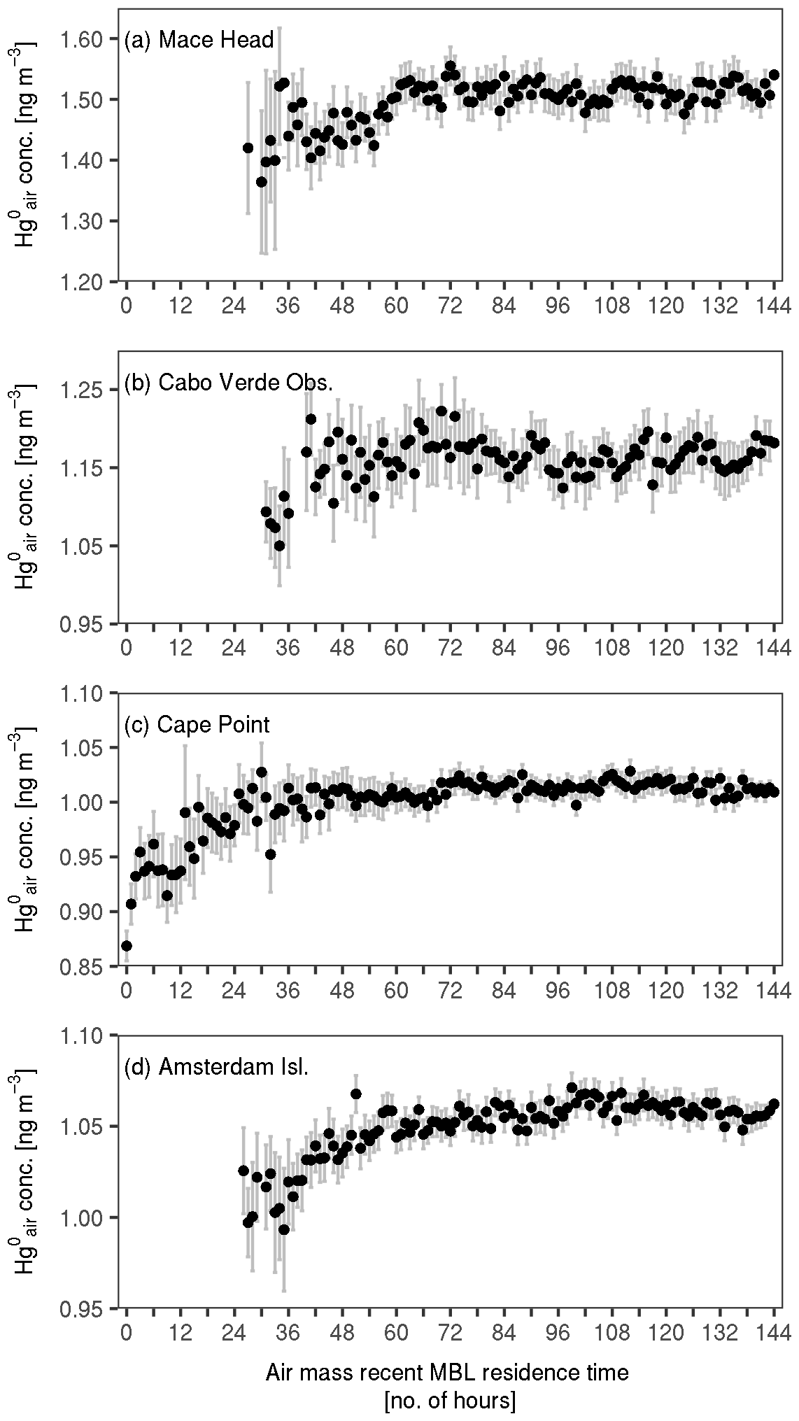
Figure 4 Mean ${\mathrm{Hg}}_{\text{air}}^{\mathrm{0}}$ concentration against air mass recent MBL residence time at the four sites. The bars show 2 times the standard error of the means. Note that the y axis differs across the four panels.

The asymptotic ${\mathrm{Hg}}_{\text{air}}^{\mathrm{0}}$ pattern is clearer at Cape Point and Amsterdam Island compared to Mace Head and Cabo Verde Observatory. A possible explanation for this is the contribution from anthropogenic emissions. As already mentioned, overall, anthropogenic Hg emissions are higher in the NH than in the SH. As such, it may be that, at Mace Head and Cabo Verde Observatory, the anthropogenic (emission) signal is strong enough that it obscures the relationship between ${\mathrm{Hg}}_{\text{air}}^{\mathrm{0}}$ concentrations and air mass recent MBL residence time. The fact that at Mace Head and Cabo Verde Observatory the asymptotic ${\mathrm{Hg}}_{\text{air}}^{\mathrm{0}}$ pattern is revealed after filtering out air masses which have had recent contact with the continental planetary boundary layer (see Appendix A) supports this hypothesis.

Nevertheless, the observed asymptotic ${\mathrm{Hg}}_{\text{air}}^{\mathrm{0}}$ increase at the sites may be partially explained by the exchange of Hg⁰ between the ocean and the atmosphere. The pattern is consistent with the air–sea gas exchange model (Eq. 1 in Sect. 3.5), which predicts net ocean Hg⁰ emissions into passing air masses until the ${\mathrm{Hg}}_{\text{air}}^{\mathrm{0}}$ concentration in them normalised by the Henry's law constant matches the surface ocean ${\mathrm{Hg}}_{\text{aq}}^{\mathrm{0}}$ concentration. While other processes may be involved, we are unable to discern them in this study. Concerning redox chemistry, our estimation of the rate of net chemical loss due to oxidation shows that it is 2 orders of magnitude lower than the rate of Hg⁰ concentration change observed here (see details in Appendix B), suggesting that the observed ${\mathrm{Hg}}_{\text{air}}^{\mathrm{0}}$ concentration increase far exceeds net oxidation-driven loss. Over longer periods, net oxidation may play a more significant role in shaping ${\mathrm{Hg}}_{\text{air}}^{\mathrm{0}}$ concentrations in the MBL. However, over the short timescale considered here, its impact on the observed patterns is negligible.

We also investigated seasonal variability in the observed relationship between ${\mathrm{Hg}}_{\text{air}}^{\mathrm{0}}$ concentrations and air mass recent MBL residence time; however, no clear pattern emerged (Fig. S7). Therefore, in the subsequent sections, where we use the observed relationship to estimate surface ocean ${\mathrm{Hg}}_{\text{aq}}^{\mathrm{0}}$ concentrations as well as ocean net Hg⁰ emissions fluxes, seasonal analyses are not included.

3.4 Estimation of surface ocean ${\mathrm{Hg}}_{\text{aq}}^{\mathrm{0}}$ concentrations

Assuming our findings in Sect. 3.3 can explain most of the variation in ${\mathrm{Hg}}_{\text{air}}^{\mathrm{0}}$ concentrations in the MBL, we used the steady-state ${\mathrm{Hg}}_{\text{air}}^{\mathrm{0}}$ concentrations in air masses reaching the sites to estimate mean surface ocean ${\mathrm{Hg}}_{\text{aq}}^{\mathrm{0}}$ concentrations. Based on the back trajectory footprints (see Fig. 5), we assume that the estimates (both the ${\mathrm{Hg}}_{\text{aq}}^{\mathrm{0}}$ concentrations and the fluxes, in Sect. 3.5 below) derived from the Mace Head and Cape Verde Observatory ${\mathrm{Hg}}_{\text{air}}^{\mathrm{0}}$ observations represent average conditions for the broad ocean area comprising the North Atlantic and Arctic oceans, while those derived from the Cape Point and Amsterdam Island data represent conditions for the area encompassing the Southern, South Atlantic and south Indian oceans. We apply the equation describing the air–sea exchange flux of Hg⁰, F, based on the thin-film gas exchange model from Liss and Merlivat (1986):

$$\begin{array}{}\text{(1)}& F=k_{\mathrm{w}}\left(H{g}_{\text{aq}}^{\mathrm{0}}-{\displaystyle \frac{H{g}_{\text{air}}^{\mathrm{0}}}{H^{\prime }}}\right),\end{array}$$

where k_w is the gas transfer velocity, ${\mathrm{Hg}}_{\text{aq}}^{\mathrm{0}}$ and ${\mathrm{Hg}}_{\text{air}}^{\mathrm{0}}$ are the surface ocean and atmospheric Hg⁰ concentrations, respectively, and H^′ is the dimensionless Henry's law constant. Following the discussion in Sect. 3.3, for air masses that remain in the MBL long enough, we can assume that they reach steady-state conditions with the underlying ocean surface, implying an average net exchange flux of F≈0 (see the discussion on the possible effect of redox chemistry in Appendix B). Note that this assumption does not imply a net zero air–sea exchange flux for the ocean as a whole, as unsaturated air masses continuously enter the MBL and take up Hg⁰ from the surface ocean. In this case, ${\mathrm{Hg}}_{\text{aq}}^{\mathrm{0}}$ is obtained with

$$\begin{array}{}\text{(2)}& {\mathrm{Hg}}_{\text{aq}}^{\mathrm{0}}={\displaystyle \frac{{\mathrm{Hg}}_{\text{air(ss)}}^{\mathrm{0}}}{H^{\prime }}},\end{array}$$

where ${\mathrm{Hg}}_{\text{air(ss)}}^{\mathrm{0}}$ is the steady-state ${\mathrm{Hg}}_{\text{air}}^{\mathrm{0}}$ concentration. H^′ is calculated using the derivation from Andersson et al. (2008a):

$$\begin{array}{}\text{(3)}& H^{\prime }=e^{\left(\frac{-\mathrm{2404.3}}{T}+\mathrm{6.92}\right)},\end{array}$$

where T is the SST. To obtain T, we extracted hourly ERA5 SSTs (Hersbach et al., 2020) corresponding to the trajectories associated with the hourly ${\mathrm{Hg}}_{\text{air}}^{\mathrm{0}}$ observations in the steady state (i.e. the observations for which air mass recent MBL residence time is greater than or equal to 60, 72, 30 and 60 h at Mace Head, Cabo Verde Observatory, Cape Point and Amsterdam Island, respectively). More details are provided in the caption of Table 1, which summarises the ${\mathrm{Hg}}_{\text{air(ss)}}^{\mathrm{0}}$, T, H^′ and resultant mean surface ocean ${\mathrm{Hg}}_{\text{aq}}^{\mathrm{0}}$ concentration for each site.

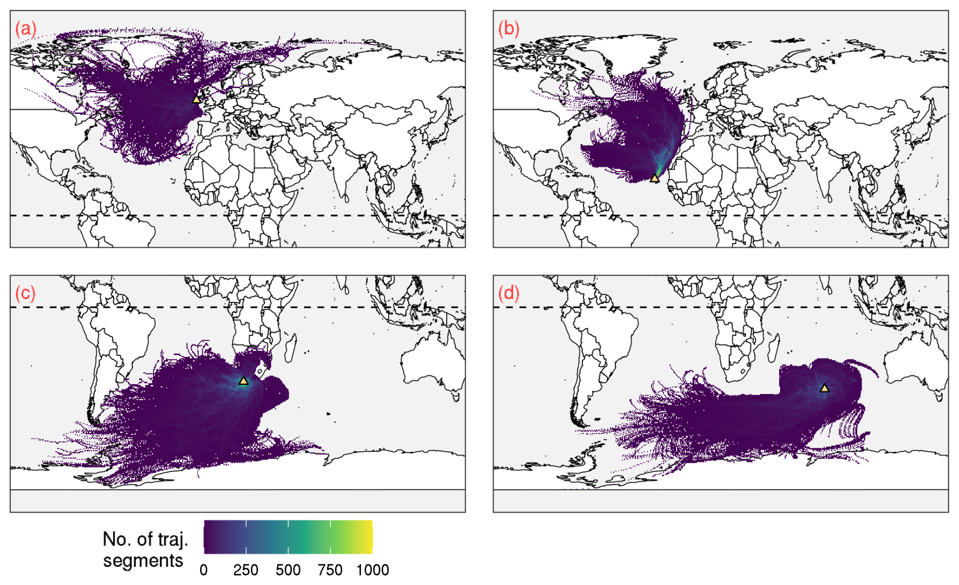
Figure 5 Back trajectory profiles illustrating the sources of air masses that arrive at (a) Mace Head, (b) Cabo Verde Observatory, (c) Cape Point and (d) Amsterdam Island. The back trajectories correspond to the data considered in deriving the profiles shown in Fig. 4, and shown here is only a subset of the data from January to December 2013. In each panel, the location of the site is illustrated by the yellow triangle, and the dotted horizontal line shows 0° latitude.

Table 1 Summary (mean ± 1 standard deviation) of steady-state ${\mathrm{Hg}}_{\text{air}}^{\mathrm{0}}$ (i.e. ${\mathrm{Hg}}_{\text{air}}^{\mathrm{0}}$(ss)) concentration, T, H^′ and resultant surface ocean ${\mathrm{Hg}}_{\text{aq}}^{\mathrm{0}}$ concentration across the four sites. For each variable at each site, the mean and standard deviation are based on the mean values of the (steady-state) MBL residence time bins. The mean value for each bin is the average of the individual values within the bin. For ${\mathrm{Hg}}_{\text{air}}^{\mathrm{0}}$(ss), these are the hourly ${\mathrm{Hg}}_{\text{air}}^{\mathrm{0}}$ observations grouped by back trajectory recent MBL residence time. The individual T values are the mean SSTs for the trajectories corresponding to the ${\mathrm{Hg}}_{\text{air}}^{\mathrm{0}}$ observations, considering only SSTs associated with segments assigned MBL. These T values are in turn used to obtain H^′ values, which, together with the ${\mathrm{Hg}}_{\text{air}}^{\mathrm{0}}$ concentrations, are used to calculate ${\mathrm{Hg}}_{\text{aq}}^{\mathrm{0}}$ concentrations according to Eq. (2).

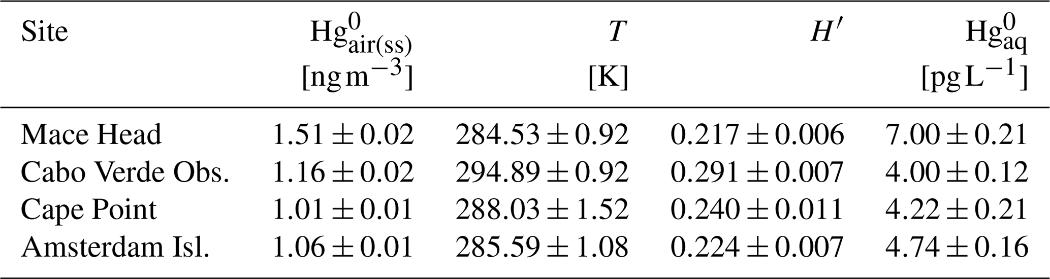
From our calculations, we derived a mean surface ocean ${\mathrm{Hg}}_{\text{aq}}^{\mathrm{0}}$ concentration of 7.00 ± 0.21, 4.00 ± 0.12, 4.22 ± 0.21 and 4.74 ± 0.16 pg L⁻¹ (mean ±1 standard deviation) based on the steady-state ${\mathrm{Hg}}_{\text{air}}^{\mathrm{0}}$ concentration at Mace Head, Cabo Verde Observatory, Cape Point and Amsterdam Island, respectively. The higher estimate for Mace Head compared to Cape Point and Amsterdam Island is in line with elevated anthropogenic Hg emissions and resultant ocean Hg enrichment in the NH relative to the SH. The estimate for Cabo Verde Observatory is lower than that of Mace Head (and closer to that of the two SH sites). This lower ${\mathrm{Hg}}_{\text{aq}}^{\mathrm{0}}$ concentration for Cabo Verde Observatory compared to Mace Head may be attributed to the much higher mean SST corresponding to the average position of the air masses sampled at the former site (294.89 ± 0.92 K at Cabo Verde Observatory compared to 284.53 ± 0.92 K at Mace Head; Table 1). While both sites receive air masses from the North Atlantic, Cabo Verde Observatory also samples tropical air masses, while Mace Head can sample polar air masses (see Fig. 5). Higher SSTs enhance ${\mathrm{Hg}}_{\text{aq}}^{\mathrm{0}}$ diffusivity, resulting in lower seawater concentrations.

We compare our estimates to reported surface ocean concentrations in the literature obtained from direct measurements. The estimates from Mace Head and Cabo Verde Observatory are compared to values from the North Atlantic and Arctic oceans, while those from Cape Point and Amsterdam Island are compared to values from the Southern and South Atlantic oceans (no published measurements are available for the Indian Ocean, to the best of our knowledge; see Dastoor et al., 2025). We acknowledge, nevertheless, that our estimates are not directly comparable to these reported measurements for several reasons (this applies for our evasion flux estimates as well, in the next section). While the combination of measurements from multiple short-term studies can capture the full variability in surface ocean ${\mathrm{Hg}}_{\text{aq}}^{\mathrm{0}}$ concentrations, individual measurement campaigns, which typically span a few days to a few weeks (see Tables 2 and 3, for example), primarily reflect transient conditions. In contrast, our estimates, which are derived from multi-year (${\mathrm{Hg}}_{\text{air}}^{\mathrm{0}}$) observations, represent long-term averages. Also note that some of the studies denote the surface water gaseous Hg measurements as dissolved gaseous mercury (DGM; e.g. Gårdfeldt et al., 2003; Wang et al., 2017), the sum of ${\mathrm{Hg}}_{\text{aq}}^{\mathrm{0}}$ and dimethylmercury (DMHg). Outside of upwelling regions (Adams et al., 2024), it has been shown that surface ocean DGM concentrations are comprised of mostly ${\mathrm{Hg}}_{\text{aq}}^{\mathrm{0}}$, with very minor (if any) contributions from DMHg (e.g. Mason and Fitzgerald, 1993; Horvat et al., 2003; Kotnik et al., 2007; Cossa et al., 2011; Bratkič et al., 2016); therefore, we assume that the surface DGM measurements, where they are denoted as such, represent ${\mathrm{Hg}}_{\text{aq}}^{\mathrm{0}}$.

Table 2 Reported surface ocean ${\mathrm{Hg}}_{\text{aq}}^{\mathrm{0}}$ concentrations as well as Hg⁰ air–sea exchange fluxes in the North Atlantic and Arctic oceans obtained from direct measurements, as well as the estimates from this study based on the relationship between mean ${\mathrm{Hg}}_{\text{air}}^{\mathrm{0}}$ concentrations and air mass recent MBL residence time at Mace Head and Cabo Verde Observatory. For the fluxes, positive (negative) values indicate net evasion (deposition).

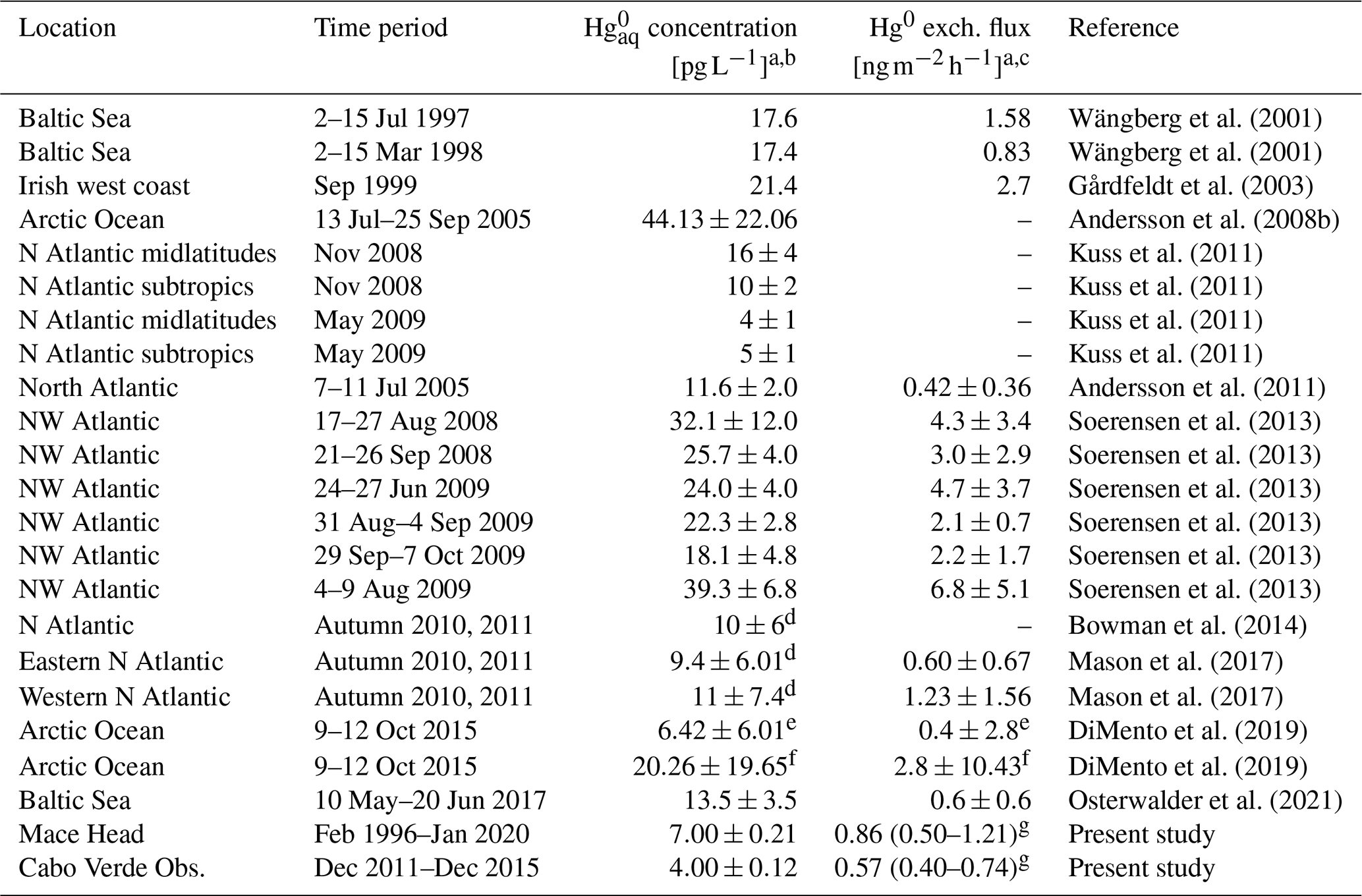
^a Mean ± standard deviation (if standard deviation given), except for our flux estimates, where we report the mean and the upper and lower bounds of the 95 % confidence interval. ^b Some concentrations reported in ng m⁻³, fM or pM and converted here to pg L⁻¹ as follows: $\mathrm{1}\mathrm{ng}{\mathrm{m}}^{-\mathrm{3}}=\mathrm{1}\mathrm{pg}{\mathrm{L}}^{-\mathrm{1}}$, $\mathrm{1}\mathrm{fM}=\mathrm{0.20059}\mathrm{pg}{\mathrm{L}}^{-\mathrm{1}}$ and $\mathrm{1}\mathrm{pM}=\mathrm{200.59}\mathrm{pg}{\mathrm{L}}^{-\mathrm{1}}$. ^c Some fluxes reported in $\mathrm{ng}{\mathrm{m}}^{-\mathrm{2}}{\mathrm{d}}^{-\mathrm{1}}$, $\mathrm{pmol}{\mathrm{m}}^{-\mathrm{2}}{\mathrm{h}}^{-\mathrm{1}}$ or $\mathrm{pmol}{\mathrm{m}}^{-\mathrm{2}}{\mathrm{d}}^{-\mathrm{1}}$ and converted here to $\mathrm{ng}{\mathrm{m}}^{-\mathrm{2}}{\mathrm{h}}^{-\mathrm{1}}$ as follows: $\mathrm{1}\mathrm{ng}{\mathrm{m}}^{-\mathrm{2}}{\mathrm{d}}^{-\mathrm{1}}=\mathrm{1}/\mathrm{24}\mathrm{ng}{\mathrm{m}}^{-\mathrm{2}}{\mathrm{h}}^{-\mathrm{1}}$, $\mathrm{1}\mathrm{pmol}{\mathrm{m}}^{-\mathrm{2}}{\mathrm{h}}^{-\mathrm{1}}=\mathrm{0.20059}\mathrm{ng}{\mathrm{m}}^{-\mathrm{2}}{\mathrm{h}}^{-\mathrm{1}}$ and $\mathrm{1}\mathrm{pmol}{\mathrm{m}}^{-\mathrm{2}}{\mathrm{d}}^{-\mathrm{1}}=\mathrm{0.20059}/\mathrm{24}\mathrm{ng}{\mathrm{m}}^{-\mathrm{2}}{\mathrm{h}}^{-\mathrm{1}}$. ^d Values from the same sampling campaign. ^e Value in ice-free open waters. ^f Value in contiguous ice-covered waters. ^g Mean and the upper and lower bounds of the 95 % confidence interval of the mean.

Table 3 Similar to Table 2, but for reported values in the South Atlantic and Southern oceans and estimates from this study for Cape Point and Amsterdam Island. Here, all reported ${\mathrm{Hg}}_{\text{aq}}^{\mathrm{0}}$ concentrations are surface ocean values except those marked with ^∗, which are total column concentrations. For the fluxes, positive (negative) values indicate net evasion (deposition).

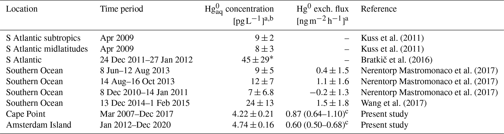
^a Mean ± standard deviation (if standard deviation given), except for our flux estimates, where we report the mean and the upper and lower bounds of the 95 % confidence interval. ^b Some concentrations reported in ng m⁻³ and converted here to pg L⁻¹ as follows: $\mathrm{1}\mathrm{ng}{\mathrm{m}}^{-\mathrm{3}}=\mathrm{1}\mathrm{pg}{\mathrm{L}}^{-\mathrm{1}}$. ^c Mean and the upper and lower bounds of the 95 % confidence interval of the mean.

Comparison of our ${\mathrm{Hg}}_{\text{aq}}^{\mathrm{0}}$ estimates to direct measurements from the literature is presented in Tables 2 and 3 for the NH and SH sites, respectively. As seen in Table 2, there is considerable variability in reported surface ocean ${\mathrm{Hg}}_{\text{aq}}^{\mathrm{0}}$ concentrations in the North Atlantic and Arctic oceans. Our Mace Head- and Cabo Verde Observatory-based estimates (7.00 ± 0.21 pg L⁻¹ and 4.00 ± 0.12 pg L⁻¹, respectively), which lie on the lower end of the reported range, are comparable to the North Atlantic concentrations from Kuss et al. (2011) (in spring, mean of ∼4–5 pg L⁻¹) and Bowman et al. (2014) (10 ± 6 pg L⁻¹), as well as the non-ice-covered Arctic Ocean concentrations from DiMento et al. (2019) (6.42 ± 6.01 pg L⁻¹), for example. The estimates are rather low compared to the values reported for the Baltic Sea by Osterwalder et al. (2021) (13.5 ± 3.5 pg L⁻¹) and Wängberg et al. (2001) (∼17 pg L⁻¹) and especially the Irish west coast (∼21 pg L⁻¹; Gårdfeldt et al., 2003), the western North Atlantic (mean values ranging between ∼18 and 39 pg L⁻¹; Soerensen et al., 2013) and the Arctic Ocean by Andersson et al. (2008b) (44.13 ± 22.06 pg L⁻¹).

The relatively high concentrations reported for the Baltic Sea, Irish west coast and western North Atlantic (from Soerensen et al., 2013), for instance, are (near-)coastal measurements and may not be representative of the open ocean. In contrast, the air masses sampled at Mace Head and Cabo Verde Observatory spent most of their time over the open ocean, and thus our ${\mathrm{Hg}}_{\text{aq}}^{\mathrm{0}}$ estimates reflect open-ocean conditions. Coastal waters typically exhibit higher Hg concentrations than the open ocean due to river inputs, which have a much stronger impact in the coastal zone compared to the open ocean (Andersson et al., 2008b; Soerensen et al., 2013; Amos et al., 2014). Similarly, the Arctic measurements from Andersson et al. (2008b) are also not representative of the non-ice-covered open ocean due to the capsulating effect of sea ice, which limits air–sea exchange, leading to the accumulation of ${\mathrm{Hg}}_{\text{aq}}^{\mathrm{0}}$ in seawater (Andersson et al., 2008b; DiMento et al., 2019).

For the SH, in situ ${\mathrm{Hg}}_{\text{aq}}^{\mathrm{0}}$ measurements are very limited. Nevertheless, for available measurements, our Cape Point (4.22 ± 0.21 pg L⁻¹) and Amsterdam Island (4.74 ± 0.16 pg L⁻¹) estimates are somewhat comparable to the values reported in the South Atlantic midlatitudes in autumn (8 ± 3 pg L⁻¹; Kuss et al., 2011). The estimates also compare well to the Southern Ocean measurements reported for summer (7.0 ± 6.8 pg L⁻¹) and winter (9 ± 5 pg L⁻¹) by Nerentorp Mastromonaco et al. (2017) but are low compared to the summer Southern Ocean measurements from Wang et al. (2017) (24 ± 13 pg L⁻¹). Bratkič et al. (2016) report total column DGM measurements for the South Atlantic, with values seemingly around 0–10 pg L⁻¹ near the surface (See Fig. 6 in Bratkič et al., 2016).

3.5 Estimation of ocean net Hg⁰ evasion fluxes

We also used the observed relationship between ${\mathrm{Hg}}_{\text{air}}^{\mathrm{0}}$ concentrations and air mass recent MBL residence time to estimate ocean net Hg⁰ evasion fluxes. The estimates are derived using a simplified Lagrangian model describing the change in Hg⁰ mixing ratio in an air parcel along a trajectory (Brasseur and Jacob, 2017). The detailed methodology is provided in Appendix B.

Based on our calculations, we estimated a mean net evasion flux of 0.86 (95 % confidence interval, CI: 0.50–1.21), 0.56 (0.40–0.74), 0.87 (0.64–1.10) and 0.59 (0.50–0.68) $\mathrm{ng}{\mathrm{m}}^{-\mathrm{2}}{\mathrm{h}}^{-\mathrm{1}}$ for the oceanic air mass source regions for Mace Head, Cabo Verde Observatory, Cape Point and Amsterdam Island, respectively (Fig. B1, Appendix B). Presented in Tables 2 and 3 are these estimates compared to reported values from the literature (calculated using in situ measurements of ${\mathrm{Hg}}_{\text{air}}^{\mathrm{0}}$ and surface ocean ${\mathrm{Hg}}_{\text{aq}}^{\mathrm{0}}$ concentrations) for the NH and SH sites, respectively.

As with the ${\mathrm{Hg}}_{\text{aq}}^{\mathrm{0}}$ concentrations, there is a large variability in reported flux estimates in the North Atlantic and Arctic oceans, with mean evasion fluxes ranging from 0 to around 7 $\mathrm{ng}{\mathrm{m}}^{-\mathrm{2}}{\mathrm{h}}^{-\mathrm{1}}$. Our Mace Head- and Cabo Verde Observatory-based estimates are comparable to values such as those reported for the Baltic Sea in winter (0.83 $\mathrm{ng}{\mathrm{m}}^{-\mathrm{2}}{\mathrm{h}}^{-\mathrm{1}}$; Wängberg et al., 2001) and summer (0.6 ± 06 $\mathrm{ng}{\mathrm{m}}^{-\mathrm{2}}{\mathrm{h}}^{-\mathrm{1}}$; Osterwalder et al., 2021), as well as the North Atlantic midlatitudes (0.42 ± 0.36 $\mathrm{ng}{\mathrm{m}}^{-\mathrm{2}}{\mathrm{h}}^{-\mathrm{1}}$; Andersson et al., 2011). The estimates are quite low compared to reported values in Irish west coast (2.7 $\mathrm{ng}{\mathrm{m}}^{-\mathrm{2}}{\mathrm{h}}^{-\mathrm{1}}$; Gårdfeldt et al., 2003) and the western North Atlantic (mean values in the range of ∼2–7 $\mathrm{ng}{\mathrm{m}}^{-\mathrm{2}}{\mathrm{h}}^{-\mathrm{1}}$; Soerensen et al., 2013).

For the SH, there are only a few flux values in the literature (Table 3). The Cape Point- and Amsterdam Island-based mean estimates from our study are within the range of Southern Ocean values reported by Nerentorp Mastromonaco et al. (2017), which show marked seasonal variability (−0.2 ± 1.3, 0.4 ± 1.5 and 1.1 ± 1.6 $\mathrm{ng}{\mathrm{m}}^{-\mathrm{2}}{\mathrm{h}}^{-\mathrm{1}}$ in summer, winter and spring, respectively). The estimates are lower than the Southern Ocean value from Wang et al. (2017) (1.5 ± 1.8 $\mathrm{ng}{\mathrm{m}}^{-\mathrm{2}}{\mathrm{h}}^{-\mathrm{1}}$).

3.6 Global extrapolation

By extrapolation of our site-specific flux results, we estimated a global mean evasion flux. For this, we assume that the mean of our Mace Head- and Cabo Verde Observatory-based estimates, 0.71 $\mathrm{ng}{\mathrm{m}}^{-\mathrm{2}}{\mathrm{h}}^{-\mathrm{1}}$ (95 % CI: 0.45–0.97 $\mathrm{ng}{\mathrm{m}}^{-\mathrm{2}}{\mathrm{h}}^{-\mathrm{1}}$), is representative of the North Atlantic and Arctic oceans (combined area: $\sim \mathrm{57.048}\times {\mathrm{10}}^{\mathrm{6}}$ km²), and the mean of the Cape Point- and Amsterdam Island-based estimates, 0.73 $\mathrm{ng}{\mathrm{m}}^{-\mathrm{2}}{\mathrm{h}}^{-\mathrm{1}}$ (0.57–0.89 $\mathrm{ng}{\mathrm{m}}^{-\mathrm{2}}{\mathrm{h}}^{-\mathrm{1}}$), is representative of the Southern, South Atlantic and Indian oceans ($\sim \mathrm{132.79}\times {\mathrm{10}}^{\mathrm{6}}$ km²). For the Pacific Ocean ($\sim \mathrm{168.723}\times {\mathrm{10}}^{\mathrm{6}}$ km²), which is not covered by our observatories, we use the mean of the four estimates, 0.72 $\mathrm{ng}{\mathrm{m}}^{-\mathrm{2}}{\mathrm{h}}^{-\mathrm{1}}$ (0.51–0.93 $\mathrm{ng}{\mathrm{m}}^{-\mathrm{2}}{\mathrm{h}}^{-\mathrm{1}}$). Under these assumptions, we obtain a global mean evasion flux of around 2270 t yr⁻¹, with a 95 % confidence interval of 1600–2900 t yr⁻¹. This flux is rather small compared to recent model estimates, which range from 2800 to 4000 Hg⁰ t yr⁻¹ (Horowitz et al., 2017; AMAP/UN Environment, 2019; Outridge et al., 2018; Shah et al., 2021; Zhang et al., 2023), suggesting that net oceanic Hg⁰ emission may currently be overestimated. Such an overestimation may relate to the parameterisation of the air–sea exchange velocity (e.g. Nightingale et al., 2000; McGillis et al., 2001) used in the models which is a large source of uncertainty (Zhang et al., 2019; Osterwalder et al., 2021).

That being said, our estimate is evidently subject to significant uncertainties, particularly due to the strong assumption that the results corresponding to individual sites and their oceanic areas of influence (see Fig. 5) are somewhat representative of larger oceanic regions. In addition, back trajectories, on which our estimate is based, provide only a general indication of air mass source regions and are prone to large uncertainties from possible errors in input meteorological fields as well as numerical models (Yu et al., 2009).

4 Summary and conclusions

In this study, we combined long-term ${\mathrm{Hg}}_{\text{air}}^{\mathrm{0}}$ observations with HYSPLIT air mass back trajectories at four ground-based monitoring sites, Mace Head and Cabo Verde Observatory in the NH and Cape Point and Amsterdam Island in the SH, to study Hg⁰ air–sea exchange. At all sites, we observed weak seasonal and diurnal ${\mathrm{Hg}}_{\text{air}}^{\mathrm{0}}$ variations, even after filtering the data to extract observations representative of MBL conditions. This suggests that the weak variations reflect actual MBL dynamics and are not an artefact of the sampling of air masses of both oceanic and terrestrial origin.

We investigated the relationship between ${\mathrm{Hg}}_{\text{air}}^{\mathrm{0}}$ concentrations and the recent residence time of air masses in the MBL. Our results showed a gradual increase in mean ${\mathrm{Hg}}_{\text{air}}^{\mathrm{0}}$ concentration with air mass recent MBL residence time, followed by a steady state. The observed pattern is consistent with the thin-film gas exchange model, which predicts net ocean Hg⁰ emissions into the atmosphere until the ${\mathrm{Hg}}_{\text{air}}^{\mathrm{0}}$ concentration normalised by the Henry's law constant matches the surface ocean ${\mathrm{Hg}}_{\text{aq}}^{\mathrm{0}}$ concentration. This provides strong evidence that ocean Hg⁰ emissions directly influence the observed ${\mathrm{Hg}}_{\text{air}}^{\mathrm{0}}$ concentrations at the sites. Combined with the weak seasonal and diurnal variability at the sites, our findings suggest that air mass recent MBL residence time has a stronger influence on ${\mathrm{Hg}}_{\text{air}}^{\mathrm{0}}$ concentrations in the MBL than seasonal and diurnal factors, such as solar radiation.

Using the relationship between mean ${\mathrm{Hg}}_{\text{air}}^{\mathrm{0}}$ concentrations and air mass recent MBL residence time at the sites, we estimated surface ocean ${\mathrm{Hg}}_{\text{aq}}^{\mathrm{0}}$ concentrations as well as ocean net Hg⁰ evasion fluxes for the North Atlantic and Arctic oceans (AA) and the Southern, South Atlantic and south Indian oceans (SSI). The estimated ${\mathrm{Hg}}_{\text{aq}}^{\mathrm{0}}$ concentration was in the range of ∼4–7 pg L⁻¹ for the AA and around 4 pg L⁻¹ for the SSI, while the mean evasion flux was around 0.6–0.8 $\mathrm{ng}{\mathrm{m}}^{-\mathrm{2}}{\mathrm{h}}^{-\mathrm{1}}$ and 0.5–0.7 $\mathrm{ng}{\mathrm{m}}^{-\mathrm{2}}{\mathrm{h}}^{-\mathrm{1}}$ for the AA and SSI, respectively. Extrapolating the fluxes to the global scale, we derived a global net Hg⁰ evasion flux of around 2270 t yr⁻¹ (95 % CI: 1600–2900 t yr⁻¹). While this global estimate is based on strong assumptions and is subject to significant uncertainties, it suggests that current model estimates of net Hg⁰ evasion flux (2800–4000 Hg⁰ t yr⁻¹) may be too high. To improve the accuracy of the flux estimate, it is crucial to conduct longer-term, higher-frequency in situ measurements of Hg⁰ air–sea exchange fluxes (as well as ${\mathrm{Hg}}_{\text{aq}}^{\mathrm{0}}$ concentrations). These efforts are particularly crucial in the SH, where direct measurements are currently very sparse. Such comprehensive measurements would significantly improve our understanding and modelling of Hg cycling in the MBL.

The methodology applied here could be improved. In particular, the air mass back trajectories could be computed with higher spatially and temporally resolved meteorological input, if enough computational resources are available. However, while higher-resolution input data could provide more accurate insights into the sources and travel paths of air masses, relatively low-resolution input data (NCEP/NCAR Reanalysis) were chosen here considering the large number of trajectories (e.g. every hour between 1996 and 2020 for Mace Head) which had to be computed for the study.

While the results of this paper are subject to significant uncertainties, our study demonstrates the applicability of ground-based ${\mathrm{Hg}}_{\text{air}}^{\mathrm{0}}$ observations, where the currently available measurements span multiple years, in studying air–sea exchange as well constraining surface ocean ${\mathrm{Hg}}_{\text{aq}}^{\mathrm{0}}$ concentrations and net ocean Hg⁰ evasion fluxes.

Appendix A: ${\mathrm{Hg}}_{\text{air}}^{\mathrm{0}}$ concentration in relation to air mass recent MBL residence time

We used the HYSPLIT air mass back trajectories to investigate the relationship between observed ${\mathrm{Hg}}_{\text{air}}^{\mathrm{0}}$ concentration and air mass recent MBL residence time. Air mass recent MBL residence time is defined as the number of hours that an air mass (corresponding to an hourly ${\mathrm{Hg}}_{\text{air}}^{\mathrm{0}}$ observation) spent in the MBL in the past 144 h before reaching the site, i.e. the number of segments of the back trajectory that are classified as MBL as per our back trajectory segment categorisation (described in Sect. 2.2). We then group together the ${\mathrm{Hg}}_{\text{air}}^{\mathrm{0}}$ observations according to air mass recent MBL residence time at an hourly temporal resolution.

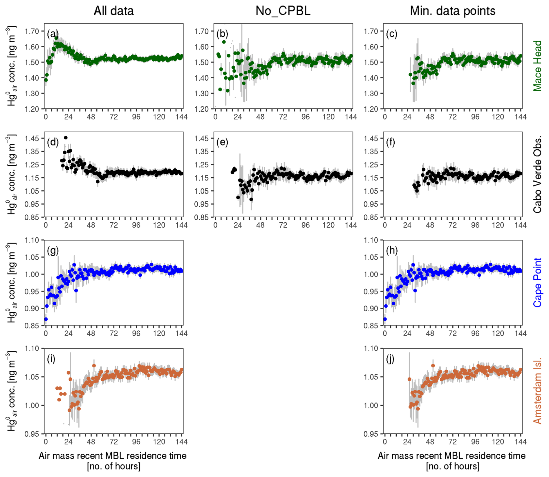
Figure A1 Mean ${\mathrm{Hg}}_{\text{air}}^{\mathrm{0}}$ concentration against air mass recent MBL residence time at Mace Head, Cabo Verde Observatory, Cape Point and Amsterdam Island, showing the progressive filtering applied. In the panel on the left (“All data”), the entire dataset is used at each site. In the middle panels (“No_CPBL”), ${\mathrm{Hg}}_{\text{air}}^{\mathrm{0}}$ data points in which the corresponding back trajectory has any segments categorised as CPBL have been removed; this is applied only at Mace Head and Cabo Verde Observatory. In the panels on the right (“Minimum data points”), the same data as on the left are used, but MBL residence times with fewer than 12 ${\mathrm{Hg}}_{\text{air}}^{\mathrm{0}}$ observations are removed. The bars show 2 times the standard error of the means. Note that the extent of the y axis differs across the four stations.

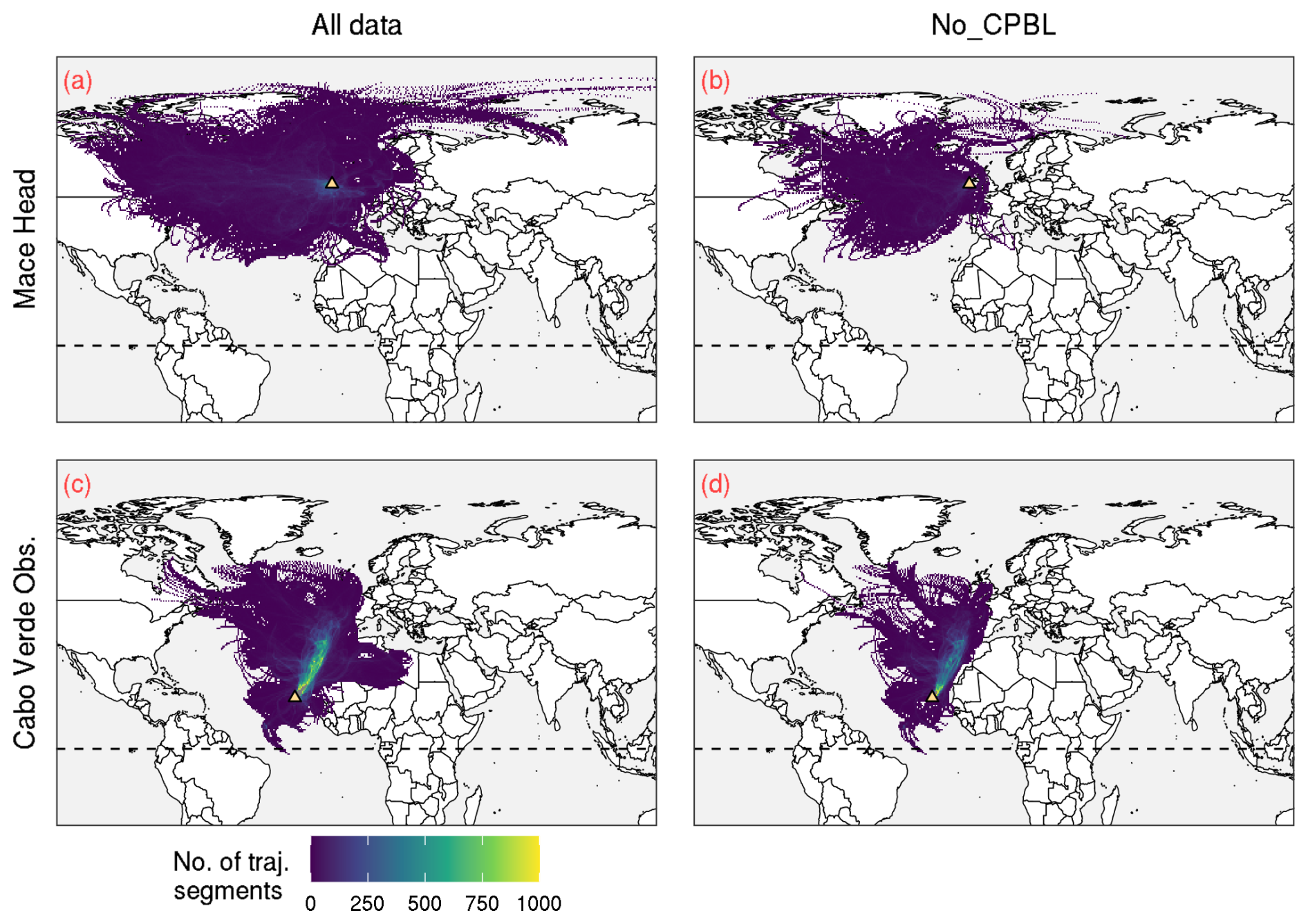
Figure A2 Illustration of the back-trajectory-based filtering applied at Mace Head and Cabo Verde Observatory, with a sample from July–December 2013. The left-side panels (a, c) show the trajectories corresponding to all data, and on the right (b, d) the trajectories which have any segments categorised as CPBL have been removed. The dashed horizontal line shows 0° latitude, and the location of the station is illustrated with the yellow triangle.

Figure A1 shows the mean ${\mathrm{Hg}}_{\text{air}}^{\mathrm{0}}$ concentrations against air mass recent MBL residence time at the four sites. The left-hand panels show the initial results. For Cape Point and Amsterdam Island (Fig. A1g and i, respectively), there is a clear pattern of increasing mean ${\mathrm{Hg}}_{\text{air}}^{\mathrm{0}}$ concentration with air mass recent MBL residence time, albeit with some outliers. At Mace Head, we observe an increase in mean ${\mathrm{Hg}}_{\text{air}}^{\mathrm{0}}$ concentration from 0 to about 14 h in the MBL, followed by a decline until about 48 h, a slight increase and then steady concentrations (Fig. A1a). Cabo Verde Observatory shows a similar pattern, with decreasing concentrations until about 60 h of MBL duration, followed by an increase until about 68 h and then mostly steady ${\mathrm{Hg}}_{\text{air}}^{\mathrm{0}}$ concentrations (Fig. A1d).

We expected the pattern observed at Cape Point and Amsterdam Island to be present at Mace Head and Cabo Verde Observatory as well, so we investigated further. Since anthropogenic Hg emissions are generally higher in the NH compared to the SH, we hypothesised that, at Mace Head and Cabo Verde Observatory, the relationship between mean ${\mathrm{Hg}}_{\text{air}}^{\mathrm{0}}$ concentrations and air mass recent residence time in the MBL is obscured by anthropogenic emissions. This would explain the relatively high mean ${\mathrm{Hg}}_{\text{air}}^{\mathrm{0}}$ concentrations at low MBL residence times at the two NH sites (Fig. A1a and d). To reduce the impact of anthropogenic emissions, we removed the hourly ${\mathrm{Hg}}_{\text{air}}^{\mathrm{0}}$ observations where the air mass recently had contact with the terrestrial surface, i.e. where the corresponding air mass back trajectory has any segments classified as CPBL (see Fig. A2 for an illustration of the trajectory filtering). These results, referred to as No_CPBL, are shown in the middle column of Fig. A1. We tested various (less strict) versions of this filter, for instance removing the ${\mathrm{Hg}}_{\text{air}}^{\mathrm{0}}$ observations where the back trajectory had a certain percentage of segments in the CPBL only in the last 6, 12 or 24 h before arrival at the site (not shown). These various filters produced more or less similar results to the No_CPBL filter.

As seen in Fig. A1b and e, reducing the influence of the terrestrial environment at Mace Head and Cabo Verde Observatory, respectively, reveals a similar pattern to that observed at the SH sites, albeit with considerable noise at the lower MBL residence time groups, particularly at Mace Head. Further investigation showed that the noisy values were due to a low number of observations in the groups (in some instances, a single data point). Therefore, we applied a 12-data-point (equivalent to half a day's observations) minimum filter, removing groups with fewer than 12 observations. This rule was applied to all sites, and the results (minimum data points) are presented in the right-hand panels of Fig. A1.

Influence of Agulhas Current region emissions at Amsterdam Island

The ${\mathrm{Hg}}_{\text{air}}^{\mathrm{0}}$ observations at Amsterdam Island show a clear pattern of increasing concentration with air mass recent MBL residence time (Fig. A1i and j). Nevertheless, there are occurrences of relatively high mean concentrations at low MBL residence time groups. We investigated these occurrences by studying the individual hourly observations in these groups. The investigation showed that for most of these occurrences, one or more of the hourly observations has an unusually high value (considering the site's mean of 1.06 ± 0.07 ng m⁻³), over 1.3 ng m⁻³. Further investigation into these unusually high concentrations showed a close association with air masses coming from the Agulhas Current region. This finding is analogous to that of Bieser et al. (2020), who observed that elevated ${\mathrm{Hg}}_{\text{air}}^{\mathrm{0}}$ concentrations at Cape Point were linked to air masses from the warm Agulhas Current region. We therefore remove all hourly observations at Amsterdam Island where the corresponding trajectory has travelled over the Agulhas Current region (Fig. A3). For Cape Point, we did not observe the same impact, and hence the same filtering was not applied.

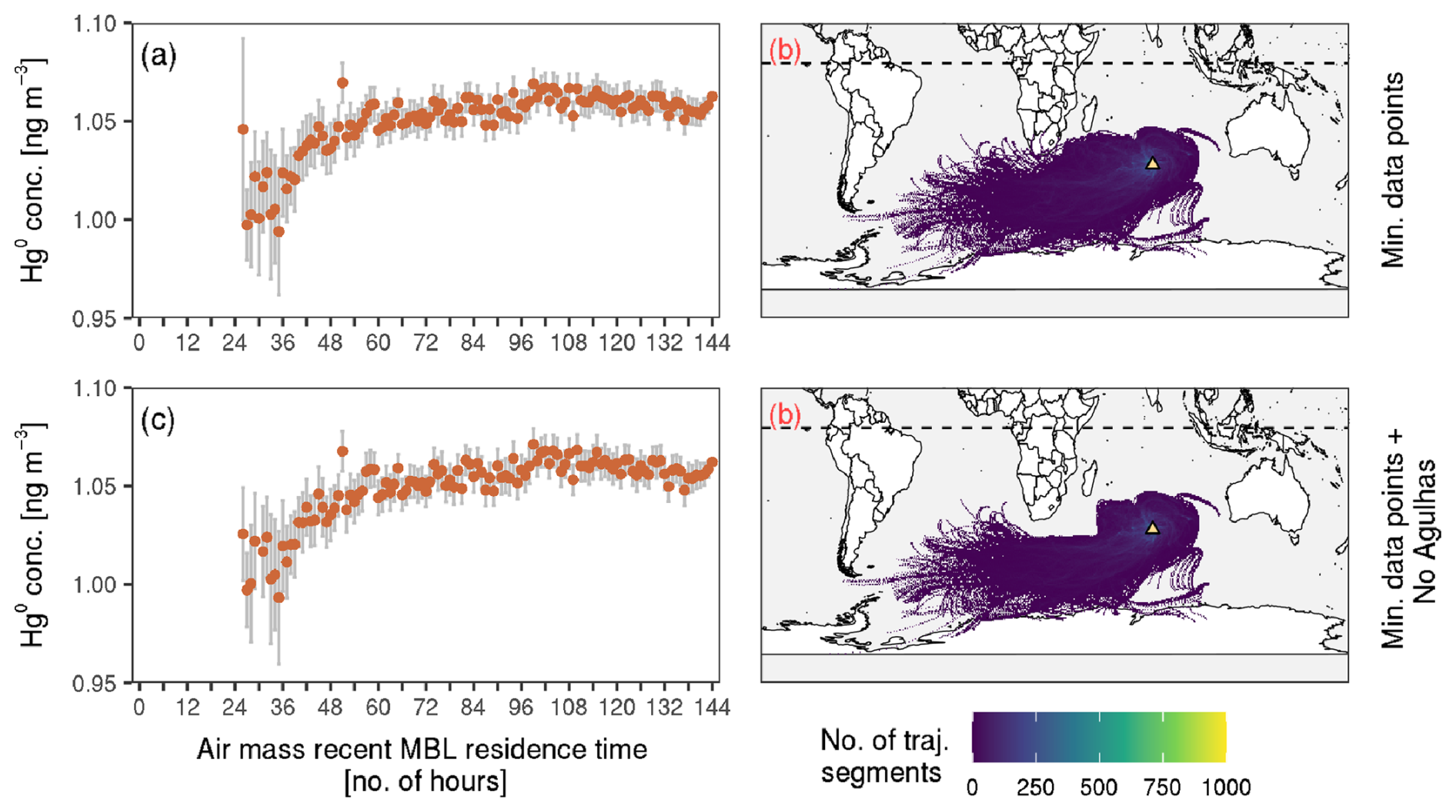
Figure A3 Illustration of the Agulhas Current filtering applied at Amsterdam Island. (a, c) Mean ${\mathrm{Hg}}_{\text{air}}^{\mathrm{0}}$ concentration against air mass recent MBL residence time and (b, d) the corresponding air mass back trajectories (a sample, January–June 2013). Panel (a) is the same as Fig. S7j, while in (c) ${\mathrm{Hg}}_{\text{air}}^{\mathrm{0}}$ observations where the back trajectory has travelled over the Agulhas Current (defined as latitude between 40 and 27° S and longitude between 20 and 50° E) have been removed (as shown in d). In panels (a) and (c) the bars show 2 times the standard error of the means. On the maps the location of the station is shown by the yellow triangle and the dotted horizontal line shows 0° latitude.

Appendix B: Constraining ocean net Hg⁰ evasion fluxes from the observed relationship between mean ${\mathrm{Hg}}_{\text{air}}^{\mathrm{0}}$ concentration and air mass recent MBL residence time

We use the observed relationship between mean ${\mathrm{Hg}}_{\text{air}}^{\mathrm{0}}$ concentration and air mass recent MBL residence time at the sites to constrain the associated mean ocean net Hg⁰ evasion fluxes. We apply the continuity equation in the Lagrangian form describing the change in Hg⁰ mixing ratio along a trajectory (Brasseur and Jacob, 2017):

$$\begin{array}{}\text{(B1)}& {\displaystyle \frac{\mathrm{d}\mathit{\mu }}{\mathrm{d}t}}={\displaystyle \frac{\mathrm{1}}{{\mathit{\rho }}_{\mathrm{a}}}}\left({\displaystyle \frac{F}{h_{\text{PBL}}}}-L\right),\end{array}$$

where $\mathit{\mu }=c/{\mathit{\rho }}_{\mathrm{a}}$ is the mass mixing ratio of Hg⁰ in air, c is the Hg⁰ air concentration and ρ_a the air density, h_PBL is the planetary boundary layer height, F is the air–sea Hg⁰ exchange flux, and L is the net chemical loss of Hg⁰. The flux F and net loss L terms are expressed according to

$$\begin{array}{}\text{(B2)}& {\displaystyle }F=k_{\mathrm{w}}\left(c_{\mathrm{w}}-{\displaystyle \frac{c}{H^{\prime }}}\right),\text{(B3)}& {\displaystyle }L=c{R}_{\text{ch}},\end{array}$$

where k_w is the gas transfer velocity, c_w is the seawater dissolved Hg⁰ concentration, $H^{\prime }=c/c_{\mathrm{w}}$ is the dimensionless Henry's law constant, and R_ch is the net chemical loss rate of Hg⁰ in the MBL.

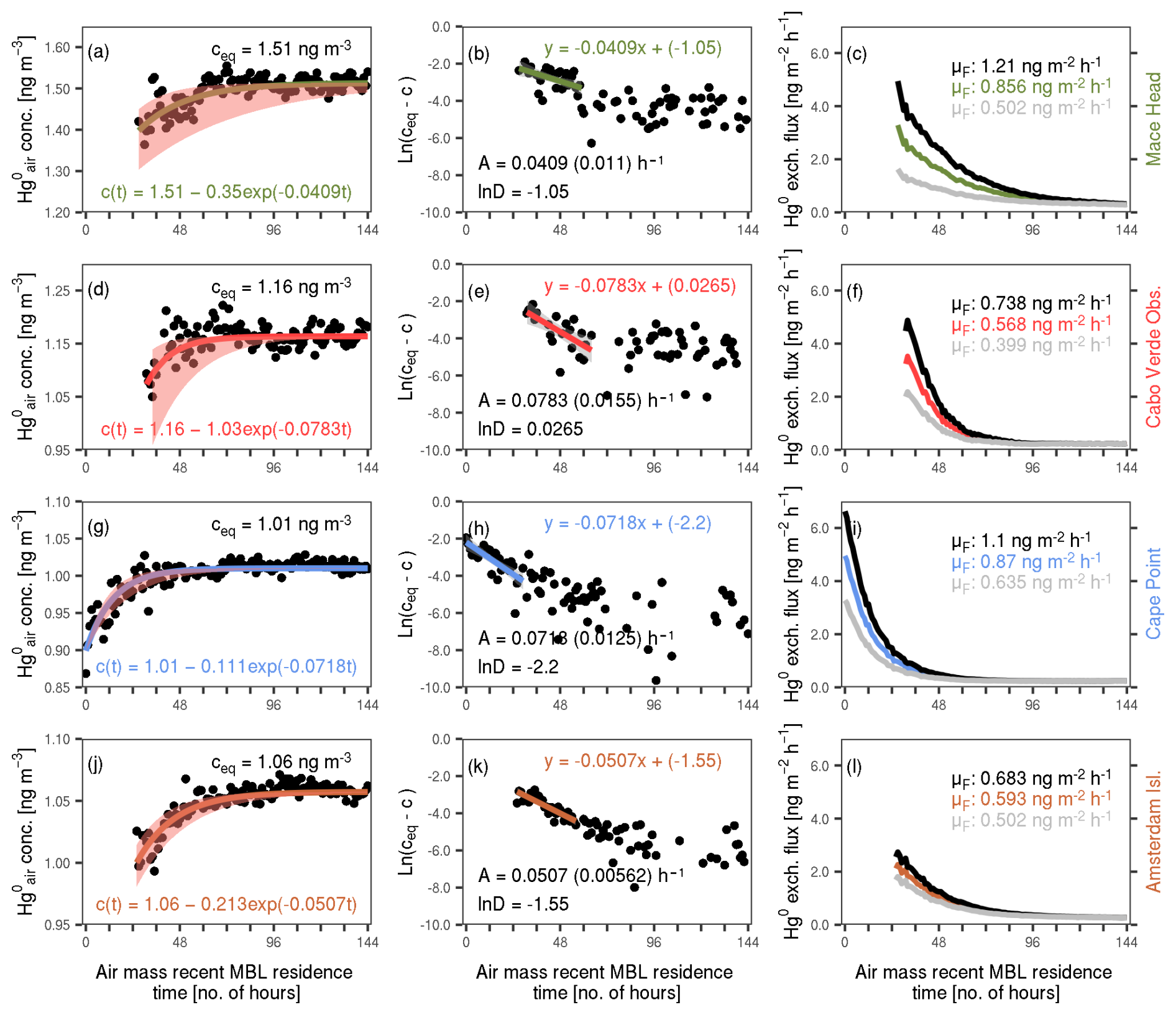
Figure B1 Sequential process of estimating mean ocean net Hg⁰ evasion fluxes from the relationship between mean ${\mathrm{Hg}}_{\text{air}}^{\mathrm{0}}$ concentration and air mass recent MBL residence time at the monitoring sites. Left-most panels (a, d, g, j): mean ${\mathrm{Hg}}_{\text{air}}^{\mathrm{0}}$ concentration against air mass recent MBL residence time (black dots), with the mean steady-state ${\mathrm{Hg}}_{\text{air}}^{\mathrm{0}}$ concentration (c_eq) and the approximation for c(t) (curve and equation) also shown. The shading gives the approximate 95 % confidence interval of c(t) (derived using A ± 2 times SE of A). Middle panels (b, e, h, k): ln (c_eq−c) against air mass recent MBL residence time. Also illustrated is the linear approximation of ln (c_eq−c) (curve and the equation) as well as the resultant A (including the SE of A, in brackets) and ln D estimates. Right-most panels (c, f, i, l): ocean net Hg⁰ evasion flux (F) against air mass recent MBL residence time. The three curves correspond to the best approximation and the upper and lower bounds of the 95 % confidence interval of F (calculated using A ± 2 times SE of A). The mean values of the curves, μ_F, are shown on the top right.

Substituting Eqs. (B2) and (B3) into Eq. (B1) and multiplying the resulting equation by air density ρ_st=1.275 kg m⁻³ at standard temperature and pressure (T_st=273.15 K, p_st=10⁵ Pa, IUPAC), we obtain the equation for Hg⁰ air concentration at standard temperature and pressure (as measured by Tekran):

$$\begin{array}{}\text{(B4)}& {\displaystyle \frac{\mathrm{d}c}{\mathrm{d}t}}=B-Ac,\end{array}$$

where $A=\frac{k_{\mathrm{w}}}{H^{\prime }{h}_{\text{PBL}}}+c{R}_{\text{ch}}$ and $B=\frac{{\mathit{\rho }}_{\text{st}}}{{\mathit{\rho }}_{\mathrm{a}}}\frac{k_{\mathrm{w}}{c}_{\mathrm{w}}}{h_{\text{PBL}}}$.

Assuming A and B are constants in the first approximation, Eq. (B4) has a solution:

$$\begin{array}{}\text{(B5)}& c\left(t\right)={\displaystyle \frac{B}{A}}-\left({\displaystyle \frac{B}{A}}-c_{\mathrm{0}}\right)e^{-At},\end{array}$$

where c₀ is the initial concentration at t=0.

Equation (B5) can be transformed to

$$\begin{array}{}\text{(B6)}& c\left(t\right)=c_{\text{eq}}-D{e}^{-At},\end{array}$$

where $c_{\text{eq}}=B/A$ is the equilibrium concentration (t→∞), and $D=c_{\text{eq}}-c_{\mathrm{0}}$.

Equation (B6) describes the temporal change in the Hg⁰ concentration (at standard temperature and pressure) in an air parcel moving along a trajectory.

We obtain c_eq by averaging the ${\mathrm{Hg}}_{\text{air}}^{\mathrm{0}}$ concentrations at the steady state. Shown in the left-most panels of Fig. B1 are the c_eq values (which are also described in Sect. 3.3 of the main text). Next, taking the natural logarithm of c_eq−c, we obtain from Eq. (B5)

$$\begin{array}{}\text{(B7)}& \ln (c_{\text{eq}}-c)=\ln D-At.\end{array}$$

Plotting ln (c_eq−c) against air mass MBL residence time and applying a linear approximation, we obtain A and ln D, as well as the standard error (SE) of A (see middle panels of Fig. B1). Using the A and ln D, we obtain the final approximation of c(t), as shown in the left-most panels of Fig. B1.

Flux estimations using the relationship between mean ${\mathrm{Hg}}_{\text{air}}^{\mathrm{0}}$ concentrations and air mass recent MBL duration

Substituting expressions for A and B from Eq. (B4) into Eq. (B2) and taking into account that $C_{\text{eq}}=B/A$, we derive

$$\begin{array}{}\text{(B8)}& F=h_{\text{PBL}}A\left({\displaystyle \frac{{\mathit{\rho }}_{\mathrm{a}}}{{\mathit{\rho }}_{\text{st}}}}{c}_{\text{eq}}-{\displaystyle \frac{A-R_{\text{ch}}}{A}}c\right).\end{array}$$

Assuming ρ_a≈ρ_st we finally obtain

$$\begin{array}{}\text{(B9)}& F\approx h_{\text{PBL}}A\left(c_{\text{eq}}-{\displaystyle \frac{A-R_{\text{ch}}}{A}}c\right),\end{array}$$

where h_PBL is the mean (ERA5-derived) planetary boundary layer height corresponding to the trajectories associated with the ${\mathrm{Hg}}_{\text{air}}^{\mathrm{0}}$ observations, considering only the trajectory segments assigned as MBL. The net chemical loss rate R_ch is determined by complex oxidation and reduction reactions of Hg° in the MBL and is difficult to evaluate directly. However, its order of magnitude can be roughly estimated using published results from chemical transport modelling. For instance, the average net chemical loss L of Hg° in the MBL can be approximately derived from Shah et al. (2021) as 1 ppq d⁻¹, which corresponds to $\mathrm{3.7}\times {\mathrm{10}}^{-\mathrm{4}}$ $\mathrm{ng}{\mathrm{m}}^{-\mathrm{3}}{\mathrm{h}}^{-\mathrm{1}}$ under standard temperature and pressure conditions. Dividing this by the average Hg° concentration of 1.5 ng m⁻³, we obtain an average net loss rate of $R_{\text{ch}}=\mathrm{2.5}\times {\mathrm{10}}^{-\mathrm{4}}$ h⁻¹. It should be noted that this value is 2 orders of magnitude lower than the estimated above values of the concentration change rate A (4–$\mathrm{8}\times {\mathrm{10}}^{-\mathrm{2}}$ h⁻¹), meaning that net chemical loss does not have a significant effect on the variation in Hg⁰ in the MBL over short timescales.

In particular, it can be easily shown that under steady-state conditions ($\mathrm{d}\mathit{\mu }/\mathrm{d}t=\mathrm{0}$) the air–sea exchange flux is close to zero, assuming an insignificant effect of redox chemistry. Indeed, from Eq. (B1) at steady state, we obtain

$$\begin{array}{}\text{(B10)}& {\displaystyle \frac{F}{h_{\text{PBL}}}}-L=\mathrm{0}.\end{array}$$

Substituting Eqs. (B2) and (B3) into Eq. (B10), expressing c_w, and substituting the expression for A from Eq. (B4), we derive

$$\begin{array}{}\text{(B11)}& c_{\mathrm{w}}={\displaystyle \frac{c}{H^{\prime }}}\left(\mathrm{1}+{\displaystyle \frac{R_{\text{ch}}}{A-R_{\text{ch}}}}\right),\end{array}$$

which simplifies to $c_{\mathrm{w}}\approx \frac{c}{H^{\prime }}$ by applying the earlier estimate R_ch≪A. Under these conditions, the air–sea flux transforms to

$$\begin{array}{}\text{(B12)}& F=k_{\mathrm{w}}\left(c_{\mathrm{w}}-{\displaystyle \frac{c}{H^{\prime }}}\right)\approx \mathrm{0}.\end{array}$$

The final approximation of F is shown in the right-most panels of Fig. B1. We assume that the coloured curves in Fig. B1 (left column) show the change in Hg⁰ concentrations during the recent (last 144 h) transport history of a typical air parcel travelling over the oceanic regions represented by our sites. To obtain the mean fluxes at each site (shown on the top right of the right-most panels), we integrated the instantaneous fluxes over the period from the shortest MBL residence time with a value to the mean MBL residence time. The integral was then normalised by the mean MBL residence time.