Vertical and horizontal variability and representativeness of the water vapor isotope composition in the lower troposphere: insight from ultralight aircraft flights in southern France during summer 2021

The isotopic composition of water vapor can be used to track atmospheric hydrological processes and to evaluate numerical models simulating the water cycle. Accurate model–observation comparisons require understanding the spatial and temporal variability of tropospheric water vapor isotopes. The challenging task of obtaining highly resolved water vapor isotopic observations is typically addressed through airborne measurements performed aboard conventional aircraft, but these offer limited microscale insights. This study uses ultralight aircraft observations to investigate water vapor isotopic composition in the lower troposphere over southern France in late summer 2021. Combining observations with models, we identify key drivers of isotopic variability and detect short-lived, small-scale processes. The key findings of this study are that (i) at hourly and sub-daily scales, vertical mixing is the primary driver of isotopic variability in the lowermost troposphere above the study site; (ii) evapotranspiration significantly impacts the boundary layer water vapor isotopic signature, as revealed by the δ¹⁸O–δD relationship; and (iii) while water vapor isotopes generally follow large-scale humidity patterns, with separation distances that might range up to 100–300 km, they also reveal distinct small-scale structures (approximately hundreds of meters) that are not fully explained by humidity variations alone, highlighting sensitivity of water vapor isotopic composition to additional fine-scale processes. The latter are particularly evident for δD, which also exhibit the largest differences in horizontal and vertical gradients. Combined with other airborne datasets, our results support a simple model driven by surface observations to simulate tropospheric δD vertical profiles, improving surface–satellite comparisons.

1 Introduction

Water vapor is one of the most important gases driving the dynamics of the Earth's climate system (Fersch et al., 2022; IPCC, 2007; Stevens and Bony, 2013). Nearly 99 % of atmospheric water vapor resides in the troposphere, where it plays a key role in the formation of clouds and the evapotranspiration process over land and oceans. Stable water isotopes are valuable for studying atmospheric water processes because phase changes influence their isotopic ratios through isotopic fractionation, hence becoming an essential tool for tracking the hydrological cycle at various spatial and temporal scales (Galewsky et al., 2016; Dee et al., 2023). In atmospheric water cycle research, the isotopic composition of water vapor is studied alongside the water vapor mixing ratio (H₂O, ppmv) or specific humidity (q, g kg⁻¹) because different processes delineate distinct patterns in the δ-humidity space. Here the δ notation expresses a relative deviation of the stable isotope ratio of a water (vapor) sample from a common reference standard in per mill units (‰) as follows:

$$\begin{array}{}\text{(1)}& \mathit{\delta }={\displaystyle \frac{R}{R_{\text{Standard}}}}-\mathrm{1},\end{array}$$

where R is the isotopic ratio of heavy to light isotopes of hydrogen (D/H for δD) and oxygen (¹⁸O/¹⁶O for δ¹⁸O), respectively, and the “Standard” subscript denotes the ratio in the international standard VSMOW (Gat, 1996). For instance, in this notation, the turbulent mixing of two air parcels with different mixing ratios and different isotopic composition is outlined by a hyperbolic shape in q, δ space, while distillation occurring during air parcel drying forms a logarithmic curve (Kendall and McDonnell, 1998; Noone 2012). A commonly used second-order parameter linked to the δD and δ¹⁸O isotopic composition of water is deuterium excess (d-excess = $\mathit{\delta }\mathrm{D}-\mathrm{8}\times {\mathit{\delta }}^{\mathrm{18}}\mathrm{O}$), which provides additional information on non-equilibrium isotopic fractionation processes. Such processes, like evaporation from a water surface, evaporation from water droplets, or condensation of ice crystals are more sensitive to the humidity gradient giving rise to a deuterium excess signature (e.g., Bolot et al., 2013; Merlivat and Jouzel 1979; Zannoni et al., 2022).

Weather regimes, surface topography and air parcel source–sink history all influence the water vapor δD, δ¹⁸O and d-excess at global and regional scales (e.g., Bonne et al., 2015; Dütsch et al., 2018; Smith and Evans, 2007; Steen-Larsen et al., 2015; Weng et al., 2021). However, uncertainties remain regarding the control of water vapor isotopic composition in the lower troposphere at meso- and microscales due to the limited number of resolving sub-hourly processes (e.g., Aemisegger et al., 2015; Graf et al., 2019), even though water cycle physics and isotope theory can provide insights on expected patterns. The number of observations of the isotopic composition of water vapor has significantly increased in the last 10 years (see, e.g., Wei et al., 2019). However, most of the recent water vapor isotope observations are sparse ground-based measurements of dedicated campaigns (e.g., Aemisegger et al., 2014; Steen-Larsen et al., 2017). Direct vertical observations in the contiguous troposphere are still scarce and challenging to obtain, especially in the boundary layer. This scarcity is indeed a limiting factor when investigating small-scale and short-lived processes of the water vapor isotopic composition. Remote sensing on satellites can provide important large-scale data that can serve as background for further small-scale investigations, providing nearly global coverage of H₂O and HDO pairs at daily resolution (see, e.g., Frankenberg et al., 2013; Herbin et al., 2007; Schneider et al., 2016; Schneider et al., 2020; Worden et al., 2006; Zadvornykh et al., 2023). However, satellite data also require validation with dedicated airborne data (Thurnherr et al., 2024).

Airborne observations are a suitable tool to investigate the horizontal and vertical distribution of water stable isotopes in the troposphere. Notable airborne measurements have been performed in the last 10 years, such as for the HyMeX project in the Mediterranean area (Sodemann et al., 2017) or over the subtropical North Atlantic Ocean for the MUSICA project (Dyroff et al., 2015) and western tropical North Atlantic for the EUREC4A project (Bailey et al., 2022). Recently, both unoccupied aerial vehicles (UAVs) and ultralight aircraft (ULA), such as ultralight trikes, have been used to observe the isotopic composition of water vapor, complementing conventional propeller-driven aircraft (Chazette et al., 2021; Rozmiarek et al., 2021). Despite challenges from large temperature variability due to the open fuselage pod and strong vibrations from proximity to the aircraft engine, ULA equipped with cavity ring-down spectroscopy (CRDS) analyzers can provide highly resolved spatial and temporal information on water vapor isotope composition over large areas (> 20 km²) within the lower troposphere (≤ 3500 $\mathrm{m}\mathrm{a}.\mathrm{s}.\mathrm{l}.$) multiple times within a day. These characteristics are essential for evaluating both the spatial and temporal representativeness of water vapor isotope composition observations in the troposphere. In this study, we utilize highly temporally and spatially resolved water vapor isotopic observations collected with an ULA during late summer 2021 in a Mediterranean climate region to provide insights into the main driving factors of the variability of water vapor isotopic composition in the lower troposphere (Zannoni et al., 2023). Specifically, our primary objective is to determine the horizontal and vertical variability of the stable water vapor isotope composition in the boundary layer and in the lowermost free troposphere. We further explore the drivers of the spatial short-lived and small-scale water isotope pattern using conceptual and numerical models and assess to which degree ground-based water isotope observations provide information about the vertical water vapor isotope structure.

Table 1 Overview of the flights performed between 17 September 2021 and 23 September 2021. Time in coordinated universal time (UTC). Altitude in meters above mean sea level ($\mathrm{m}\mathrm{a}.\mathrm{s}.\mathrm{l}.$).

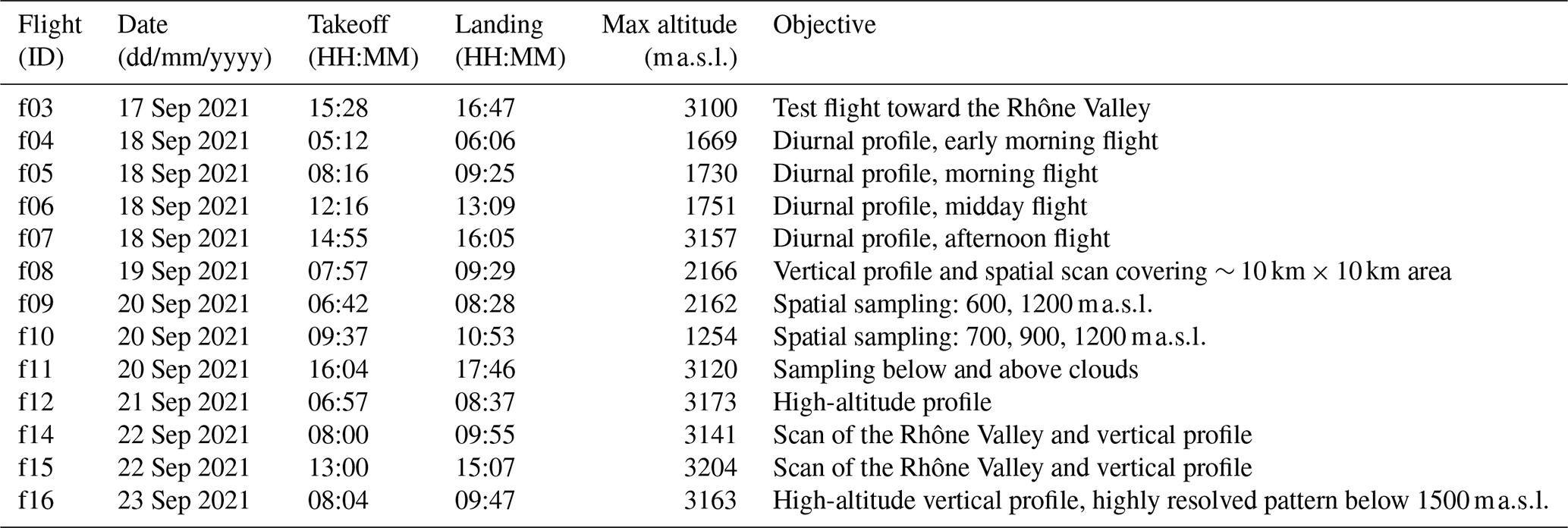
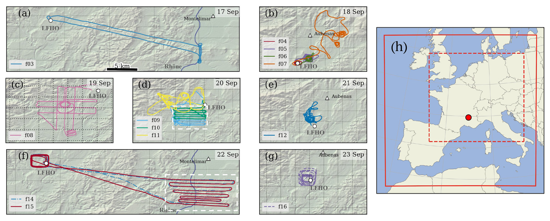
Figure 1 ULA flights f03 to f16 over the area of Aubenas (Aubenas Aerodrome) on each flying day in September 2021 (a–g). The airfield area is depicted in all the panels as a white circle (LHFO). The towns of Aubenas and Montélimar are reported for reference as white triangles. The Rhône Valley is visible on the east side of the map in panels (a) and (f) (Rhône river reported as a blue line). The areas of study cases for flights detailed in Sects. 3.6 and 3.7 are depicted with white dashed lines in panels (d) and (f). Horizontal scale reported in panel (a) (5 km) is valid for panels (a)–(f). (h) Geographical location of the Aubenas Aerodrome in France and COSMO_iso domains for coarse (0.1° × 0.1°, solid red) and fine (0.02° × 0.02°) resolutions.

2 Materials and methods

2.1 Study site and flight overview

From 17 to 23 September 2021, 13 flights were performed with an ULA near Aubenas (southern France) to probe the vertical and spatial structure of the isotopic composition of water vapor in the boundary layer and lowermost free troposphere (Table 1 and Fig. 1). Takeoff, landing and ground operations were conducted next to the Aubenas Aerodrome (ICAO: LFHO). LFHO is located on the top of a plateau bordering the west side of the Rhône Valley. The area is surrounded by low-altitude hills and mountains and is characterized by a Mediterranean climate. During the study period, the minimum and the maximum temperatures were 16 and 30 °C, respectively. Even though convective thunderstorms passed the area, only a single low-intensity precipitation event was recorded at the site during the night between 18 and 19 September 2021. Wind conditions only prevented flight operations on 19 September 2021 in the afternoon, when southerly winds of up to 14 m s⁻¹ prevailed.

2.2 Water vapor isotopic composition measurements

A Tanarg 912 XS ULA (Air Création, flown by Tignes Air Experience) was equipped with a CRDS water vapor isotope analyzer from Picarro (model L2130-i, s/n HIDS2254, hereafter CRDS analyzer). The CRDS analyzer is the same as that used in Chazette et al. (2021) and was placed on the back seat of the ULA. To minimize the effect of the large ambient temperature variability on the CRDS analyzer performances, the analyzer was wrapped with a layer of 3 mm thick neoprene sheet (RS 733-6757). A foldable aperture was made on the wrapping sheet to ensure air ventilation on the backside of the instrument. Ambient air was sampled by the CRDS analyzer in flight mode at a nominal flow rate of 80 sccm min⁻¹ through an unheated inlet of 80 cm length ($\mathrm{1}/\mathrm{4}$ in. o.d. stainless steel with Silconert coating) pointing backward on the right side of the aircraft. Despite the lack of inlet heating, no evidence of condensation was observed in the isotope data. This is likely due to the short length of the inlet, resulting in minimal air residence time within the system, as well as the ULA's infrequent exposure to high-relative-humidity conditions. The CRDS analyzer was set in flight mode, which enabled us to measure water vapor volume mixing ratio (H₂O, ppmv), δ¹⁸O and δD (‰) at ∼ 4 Hz sampling rate, hence more responsive than the conventional operating mode (∼ 40 sccm min⁻¹, ∼ 1 Hz). H₂O (ppmv) was converted to specific humidity q (g kg⁻¹) following Vaisala (2023). For both VSMOW-SLAP and humidity-isotope dependency calibration, the inlet was connected with a three-way valve to a water vapor generation module that allowed the injection of water isotope standards for q ranging between 0.6 and 12 g kg⁻¹ (Steen Larsen and Zannoni, 2024). Three water isotope standards provided by FARLAB, University of Bergen, were used every day, bracketing all the potential isotopic variability in water vapor isotopic composition in the lower troposphere of the study area. The reader is referred to Table S1 in the Supplement for details on frequency of usage, values of isotope standards and calibration performances of the CRDS analyzer. Four characterization curves were performed to check the consistency of the humidity-isotope dependency between laboratory test and field deployment (not reported). Calibration of q was performed once in the range 1.2–12 g kg⁻¹ using a calibrated chilled mirror hygrometer (Panametrics OptiSonde) as the reference instrument. The dry air source was obtained with a dry air compressor (cleanAIR CLR 20/25) equipped with an extra drying cartridge in series (Agilent MT400-4). The humidity level of the provided dry air was < 0.06 g kg⁻¹.

2.3 Estimation of precision and accuracy of water vapor isotope observations

A 90 min injection of BERM standard on 22 September was used to investigate the instrument precision in stable condition on the field with the ULA engine turned off. The first 30 min of the injection was discarded to ensure an acceptable removal of the memory effect in the inlet. The remaining 60 min was used to run an Allan deviation (ADEV) test at q = 8.3 ± 0.3 g kg⁻¹, yielding a 0.25 s ADEV of 0.20 ‰, 0.74 ‰ and 1.87 ‰ for δ¹⁸O, δD and d-excess, respectively, and a 1 s ADEV of 0.10 ‰, 0.38 ‰ and 0.95 ‰ for δ¹⁸O, δD and d-excess, respectively (for figure, see Fig. S1 in the Supplement), typical of L2130-i series. However, these values cannot be used as a reference for the precision of the instrument in flight conditions. Given that the L2130-i model uses peak absorption height for the spectral fitting, the precision of the instrument is highly sensitive to pressure broadening caused by vibrational noise transmitted by the ULA engine. As an example, Fig. S2 in the Supplement shows how cavity pressure, δ¹⁸O and d-excess measurement noise increase when the ULA engine was turned on just before takeoff for flights 7, 8 and 9. Assuming that the isotopic composition of atmospheric water vapor did not change significantly 30 s before and 30 s after turning on the engine, the standard deviations of δ¹⁸O, δD and d-excess calculated over 1 min provide insights on the decrease of instrumental precision due to engine vibrations. The standard deviations with the engine off (on) resulted in 0.22 (0.45) ‰, 0.78 (0.99) ‰ and 1.92 (3.54) ‰ for δ¹⁸O, δD and d-excess, respectively, at q = 8.2 ± 0.4 g kg⁻¹. Assuming white noise for an averaging time between 0.25 and 10 s, it is possible to normalize the results of the ADEV for when the engine is running, yielding a 1 s ADEV of 0.23 ‰, 0.50 ‰ and 1.78 ‰ for δ¹⁸O, δD and d-excess, respectively. These ADEV values can therefore be assumed representative of the instrumental precision at a 1 s averaging time and at q = 8.2 g kg⁻¹ in the taxi to runway phase. On this latter point, it is worth noting that our approach does not adequately probe all vibrational modes; hence instrumental precision might be worse. Indeed, instrument performances should be evaluated under all normal operating conditions to obtain the full spectrum of vibrational noise (AC no. 20-66, 1970).

Similarly, the 0.25 s standard deviations for δ¹⁸O, δD and d-excess measured during each step of the humidity-isotope characterization curves were scaled for an averaging time of 1 s and accounting for engine vibrations (Fig. 2). Instrumental precision can therefore be considered constant between 4–12 g kg⁻¹, with a rapid decrease at low humidity (σ_1 s is 0.7 ‰, 2.9 ‰ and 8.0 ‰ at q = 1 g kg⁻¹ for δ¹⁸O, δD and d-excess, respectively).

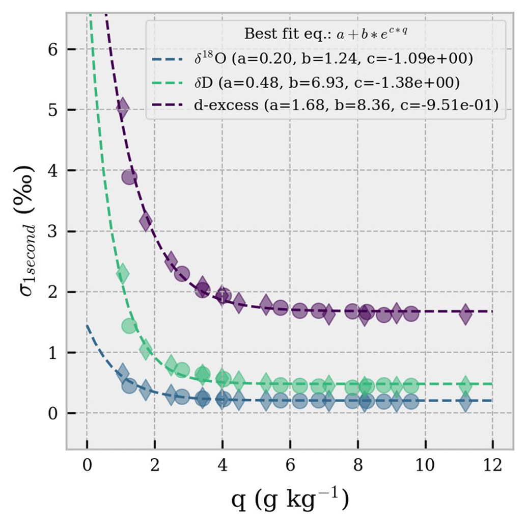
Figure 2 Precision of the CRDS analyzer as a function of humidity affected by ULA engine vibrations at ground level. Circles and diamonds represent data from GLW humidity-isotope characterization performed on 19 and 20 September, respectively. Dashed lines are the best-fit curves.

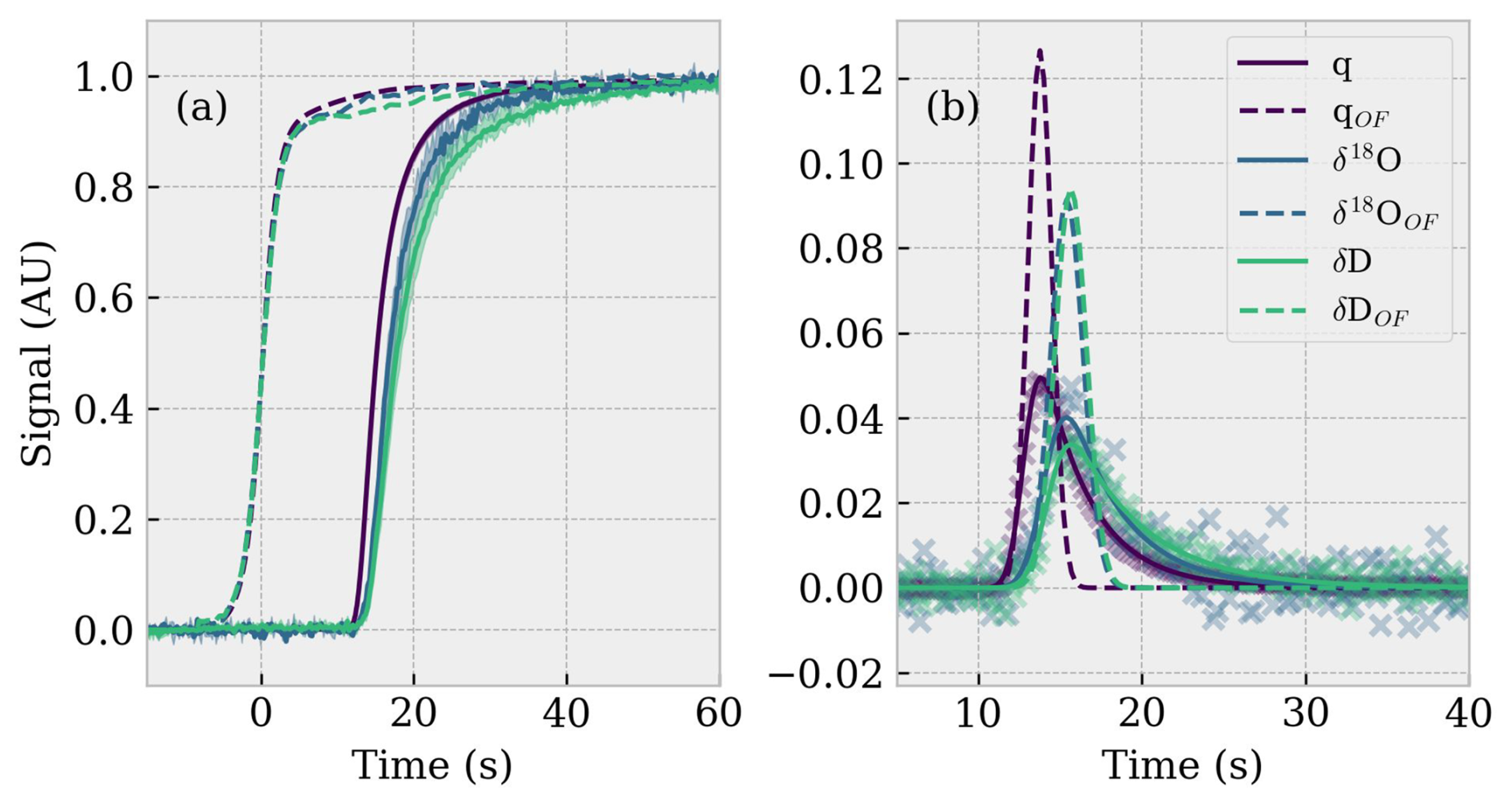
Figure 3 Analysis of the response of the CRDS analyzer to a Heaviside step function in q and the change in isotopic composition. (a) Min and max normalized step change (arbitrary units, AU) for q, δ¹⁸O and δD (averaged over three repetitions). Solid lines and shadings are average ± 1 standard deviation of raw observations of the three repetitions, respectively. Dashed lines represent filtered and sync data. Origin of the horizontal axis set when the three-way valve was switched from ambient air to the calibration line. (b) Exponentially modified Gaussian (EMG) best fit of the first derivative of the observed step changes (solid lines). Gaussian impulses with the same areas of EMG impulses (dashed lines).

2.4 Postprocessing of the water vapor isotopic composition signal: time response correction

The measuring system of the isotopic composition of water vapor is characterized by its own response time, which in turn depends on the inlet design as well as on the characteristics of the CRDS analyzer itself (Aemisegger et al., 2012; Steen-Larsen et al., 2014). When working with high-frequency data such as for airborne measurements, it becomes important to consider the response time of the measuring system. Indeed, different response times for q, δ¹⁸O and δD can introduce artifacts when looking at a combination of the signals (e.g., q vs. isotopes, or δ¹⁸O vs. δD for d-excess). The impulse response of the system was estimated by inducing a large humidity and an isotope step change and by performing the spectral analysis of its first derivative. Briefly, using a three-way valve operated by the CRDS analyzer software, the inlet source was switched between ambient air and dry air for humidity analysis and between ambient air and standard water vapor for isotope analysis at the same humidity level (Fig. 3a). The test was repeated three times. The raw data of the CRDS analyzer were studied at the sampling frequency of the analyzer (4 Hz) to avoid any possible artifacts introduced by applying a running average or by data resampling.

First, the delay introduced by the inlet + analyzer was estimated by measuring the time required to observe a deviation of the signal larger than 2σ when compared to the previous average state. Such delay was estimated to be 13.75 ± 0.05, 15.36 ± 0.27 and 15.60 ± 0.13 s for q, δ¹⁸O and δD, respectively. Second, the first derivative of the normalized step change was fitted with an exponentially modified Gaussian (EMG) distribution to perform the fast Fourier transform and to investigate the impulse response of the system (Fig. 3b). The result of the fit shows that peaks for q, δ¹⁸O and δD are not symmetrical. In analogy with chromatography (Kalambet et al., 2011), the EMG can explain the peak shape by the convolution of two distinct physical processes: mixing (Gaussian) and absorption/desorption of tubing and cavity walls (exponential). In this context, the EMG peaks were transformed into the desired Gaussian peaks by maintaining the same Gaussian σ, estimated with EMG fit, and the same area under the peak. An optimal filter (OF) was then designed by calculating the ratio of the transfer functions of EMG and Gaussian peak and by applying a first-order Butterworth low-pass filter to remove ringing (frequency cutoff: 0.1 Hz). The effect of optimal filtering and synchronization of rising edges is reported as dashed lines for q, δ¹⁸O and δD in Fig. 3a. The data used in this study are corrected as described above and correspond to fields with an “_OF” extension in the Zannoni et al. (2023) dataset, where both uncorrected and corrected measurements are available.

2.5 Meteorological observations and position data

The ULA was equipped with an iMet XQ-2 probe (InterMet systems, s/n 61124) measuring temperature (T, °C), humidity (RH, %), pressure (P, hPa) and GPS position at 1 Hz. The probe was installed on the wing mast, ensuring excellent ventilation and easy maintenance. After postprocessing q, δ¹⁸O and δD signals (Sect. 2.4), no further alignment was required between the CRDS q and the iMet humidity data. The synchronization between GPS and CRDS was achieved via pressure readings, leveraging the CRDS analyzer's built-in atmospheric pressure sensor, which offered a rapid response time (∼ tens of milliseconds), making it preferable over humidity-based synchronization. Several other meteorological parameters were acquired from ERA5 reanalyses, available on the Copernicus Climate Data Store (CDS) (Hersbach et al., 2023). Boundary layer height (BLH, m), dew point temperature (d2m, K) and surface pressure (sp, Pa) were retrieved from ERA5 hourly data on single levels. For data on single levels, the reanalysis data were interpolated to the Aubenas Aerodrome coordinates. More specifically, the BLH variable was adjusted accounting for geopotential (z, m² s⁻²) to allow comparison with flight altitude ($\mathrm{m}\mathrm{a}.\mathrm{s}.\mathrm{l}.$). Air temperature (t, K) and specific humidity (q, kg kg⁻¹) data were also retrieved as hourly data on pressure levels (37 levels).

2.6 Spatial correlation indexes and spatial representativeness of the data

The spatial structure of the water vapor mixing ratio and its isotopic composition are investigated by means of the variogram and of Moran's I spatial autocorrelation index. The variogram is a tool used to describe the variability (semivariance) between pairs of data points that are separated by a certain lag distance in the 3D space. If a spatial structure exists in the data, the observed semivariance can be explained by means of a statistical model (experimental variogram), and the variable of interest can be predicted in between non-observed locations. The experimental variogram usually starts from a non-zero value (the nugget term) and increases until reaching a plateau (the sill term) within a certain distance (the range term, set at 95 % of the sill). Using such terminology, the range can be understood as the maximum distance at which observations are correlated. Several models can be used to fit the observed semivariance; in this study we used the spherical model, which is the standard choice when fitting the empirical variogram using the Python package SciKit-GStat (Mälicke, 2022). Moran's I, on the other hand, is a statistical test to measure the degree of spatial autocorrelation (also reported as the Global Moran's I, ESRI 2024). Its null hypothesis is that the variable under investigation is randomly distributed in the study region. Hence, similarly to the Pearson correlation index, Moran's I ranges between −1 and 1, where −1 indicates that observations tend to be dispersed and 1 indicates the tendency of observations toward clustering. A Moran's I value close to 0 indicates the absence of spatial autocorrelation. The Python package PySAL has been used to estimate Moran's I by attributing spatial weights with the distance band method (Rey and Anselin, 2007).

2.7 Conceptual models describing the vertical profile water vapor isotopic composition

To simulate the vertical profile of water vapor isotopic composition, two conceptual models were used: a Rayleigh distillation model and a binary mixing model. Both conceptual models are widely used for describing and generalizing the variability of the isotopic composition of atmospheric water vapor. The reader is referred to the literature for a full description of their validity and their mathematical derivation (Galewsky et al., 2016; Gat, 1996; Noone, 2012, and references therein). Specifically, here we report only the principal assumptions behind the two approaches, and we refer to equations in Noone (2012) for both models.

In the Rayleigh model the decrease in air temperature due to adiabatic lift in saturated conditions (RH = 100 %) drives the reduction of the saturation vapor pressure of the air. Under the assumption that excess water is completely removed immediately after the phase change, the isotopic ratio of the remaining water vapor follows a logarithmic curve whose shape is given by the temperature-dependent equilibrium fractionation factor between vapor and liquid or vapor and ice (Eq. 12 as seen in Noone, 2012). The average of the observations collected with the ULA at the lowest model level for each flight was used as the initial conditions for the Rayleigh model.

In the binary mixing model, the only process involved is the turbulent mixing between two end members: dry air coming from the free atmosphere and the water vapor flux from the surface (evapotranspiration). The main point of this model is that no isotopic fractionation is involved in the process. Mixing will make humidity and isotopic composition tend toward a well-mixed state with a hyperbolic curve connecting those two extreme values. An important assumption in this model is that vertical mixing between layers is the only active process. The average of the observations collected with the ULA at the highest level available for each flight was used as representative of the dry end member (q₀ and δ₀ as seen in Noone, 2012, Eq. 23). A linear fit between the upper (drier) end member and the average of the observations at the lowest level (moist) was used to identify the flux composition (δ_F as seen in Noone, 2012, Eq. 23). Finally, for each flight and for both models the atmospheric column above the study area was discretized into 20 evenly spaced layers, from 300 to 3300 m with a 150 m constant layer height.

2.8 COSMO_iso simulations

In addition to conceptual models, the isotope-enabled regional weather prediction model COSMO_iso (Pfahl et al., 2012) was used to investigate the vertical and spatial structure of the isotopic composition of water vapor. Two additional water cycles for the heavy water molecules ${\mathrm{H}}_{\mathrm{2}}^{\mathrm{18}}\mathrm{O}$ and HD¹⁶O, respectively, are implemented in COSMO_iso to simulate the isotopic composition of the atmospheric water cycle. The additional water cycles behave analogously to the ${\mathrm{H}}_{\mathrm{2}}^{\mathrm{16}}$O water cycle and, additionally, include isotopic fractionation during phase change processes. A 10 d COSMO_iso simulation from 15 to 24 September 2021 at 0.1° (∼ 10 km) horizontal resolution and a 5 d simulation from 16 to 21 September 2021 at 0.02° resolution (∼ 2 km) have been conducted. The domain of the coarser simulation is centered around Aubenas and covers western Europe including the Mediterranean and Baltic seas and the western Atlantic eastwards of approximately −14° E (Fig. 1h). The 2 km COSMO_iso domain lies within the 10 km domain covering France and adjacent coastal ocean basins. The simulations were performed with 41 vertical levels, coupled to the isotope-enabled land module TERRA_iso including prognostic isotopic compositions of terrestrial water reservoirs (Dütsch, 2016; Christner et al., 2018), and with a model time step of 30 s for the 10 km and 20 s for 2 km simulation, respectively. The COSMOiso fields are output at a 1-hourly resolution. 6-hourly outputs from the global, isotope-enabled atmosphere model ECHAM6-wiso (Cauquoin and Werner, 2021) provided the initial and boundary conditions. The ECHAM6-wiso wind fields were spectrally nudged to the COSMO_iso simulations above 850 hPa to ensure a good representation of the large-scale flow in the regional simulations. The global ECHAM6-wiso simulation was conducted at a horizontal resolution of 0.9°, with 95 vertical levels, and was spectrally nudged to ERA5 reanalysis data (Hersbach et al., 2020).

The representation of convection in numerical simulations depends on the grid-scale and chosen parameterizations. At a horizontal resolution on the order of 10 km or less, COSMO (Steppeler et al., 2003) simulations with explicitly resolved convection resulted in a better representation of precipitation distribution over Europe than simulations with parameterized convection (Vergara-Temprado et al., 2019). Further, COSMO_iso simulations with and without convection parameterization showed a good agreement in the isotopic composition of water vapor with satellite observations over West Africa (de Vries et al., 2022). We therefore performed both COSMO_iso simulations with explicit convection in accordance with previous studies (e.g., Villiger et al., 2023; Thurnherr et al., 2024).

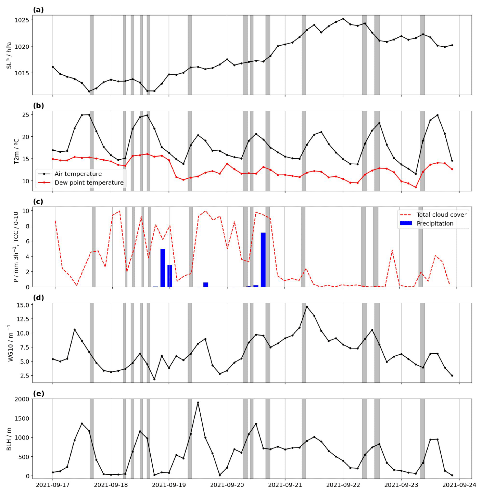
Figure 4 Evolution of weather parameters from ERA5 at the grid point closest to Aubenas compared to an automatic weather station in Montélimar (ca. 20 km distance in the Rhône Valley). Gray shading indicates flight periods. (a) Pressure at mean sea level from ERA5 (hPa, dots) and AWS (hPa, squares), (b) air temperature at 2 m (°C, black) and dew point temperature at 2 m (°C, red) from ERA5 and from AWS (°C, squares), (c) surface precipitation (mm 3 h⁻¹, bars) and total cloud cover ($\mathrm{1}/\mathrm{10}$ s, red dashed line), (d) wind gusts at 10 m (m s⁻¹), and (e) atmospheric boundary layer height (m). Note that an offset of 9 hPa was added to the AWS MSL at Montélimar for easier comparison.

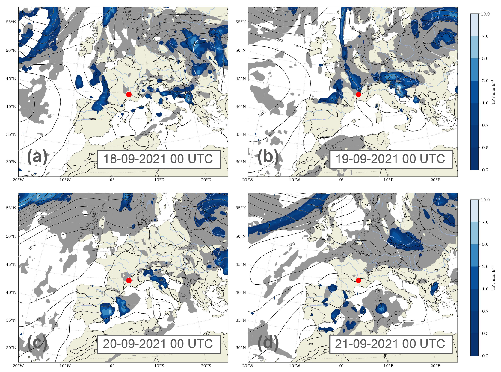
Figure 5 Total precipitation (blue shading, mm h⁻¹), total cloud cover (gray shading, 0.9 and above) and sea-level pressure (contour interval 4 hPa) from ERA5 at (a) 00:00 UTC on 18 September 2021, (b) 00:00 UTC on 20 September 2021, (c) 00:00 UTC on 21 September 2021 and (d) 00:00 UTC on 22 September 2021.

3 Results

3.1 Weather situation during the campaign

The overall weather situation during the campaign period can roughly be divided into three phases. During the first phase from 15 to 18 September, southeastern France was in between the influence of North Atlantic air masses belonging to a frontal system west of the British Isles and a high-pressure area east of Portugal (Fig. 5a). This period was characterized by low winds and generally low cloudiness (Fig. 4c), as well as a large diurnal temperature amplitude with up to 25 °C daily maximum temperatures (Fig. 4b). On 18 September, the frontal band had broken apart, shedding a short-wave trough over the Gulf of Biscay, which was then associated with intense showers over southern France during the night from 18 to 19 September (Fig. 4c). This precipitation initiated the second phase, lasting from 19–20 September (Fig. 5b). Inflowing North Atlantic air led to overall cooler temperatures with daily maxima of 20 °C, characterized by more overcast and rainy periods (Fig. 4b and c). The phase ended after an intense convective rainfall event during the midday of 20 September. Thereafter, a strengthening of the anticyclone over the Azores extending towards the English Channel (Fig. 5c and d) led to a mostly cloud-free period with increasing diurnal temperature amplitudes of up to 12 °C (Fig. 4b). Wind gusts reached up to 15 m s⁻¹ on 21 September, slowly decreasing over the next days until 24 September (Fig. 4d). The ERA5 boundary layer height shows clear diurnal cycles, reaching typically 1000–2000 m above ground (Fig. 4e).

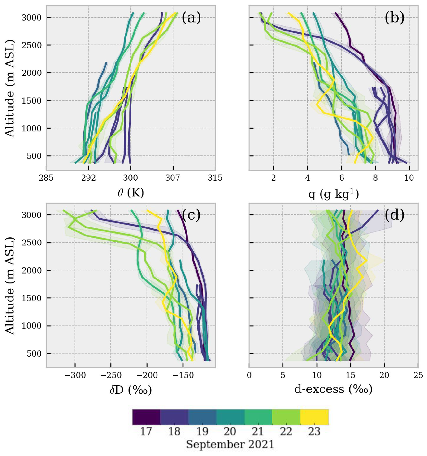
Figure 6 Vertical profiles of potential temperature (a), specific humidity (b), water vapor δD (c) and d-excess (d). Solid line represents the average calculated over a 150 m bin size. Shadings represent ± 1σ interval around the mean.

3.2 Observed daily and sub-daily vertical profiles of the water vapor isotopic composition: comparison with COSMO_iso

We now investigate the time evolution of the vertical profile measurements from the ULA during the campaign period. Figure 6 shows 150 m binned vertical profiles of potential temperature, specific humidity and water vapor isotopic composition (δD and d-excess). δ¹⁸O is not reported in Fig. 6 but is discussed in the text. The potential temperature profiles depict a stable atmosphere for most of the flights above ∼ 1200 m. The binned values of specific humidity and isotopic composition fall within a range of [1.1, 9.3] g kg⁻¹, [−40.91, −15.79 ] ‰, [−315.59, −114.25] ‰ and [9.1, 19.1] ‰ for q, δ¹⁸O, δD and d-excess, respectively. The general decrease of the mixing ratio and δD as a function of altitude is clearly visible. However, the specific humidity decrease with height is rather uniform and mirrors the general potential temperature increase up to 3000 m (for air temperature, see Fig. S3e in the Supplement).

A pronounced change in δD is visible at ∼ 2500 m altitude. Using 2500 m as a cutoff altitude, it is possible to define the isotopic lapse rate for δ¹⁸O and δD, which yields −0.20 ± 0.14 ‰ 100 m⁻¹ and −1.5 ± 1.2 ‰ 100 m⁻¹. These isotopic lapse rates are fully comparable to vertical gradients observed for surface precipitation as a function of the altitude of several sampling stations in the Mediterranean region (see, e.g., Balagizi and Liotta, 2019; Masiol et al., 2021).

Below 2500 m, d-excess shows no particular feature for all the flights despite the large RH variability observed (Fig. S3f in the Supplement). Among the flights which reached altitudes > 3000 m (flights 3, 7, 11–16), only flight 7 exhibits a consistent positive deviation of d-excess from the mean value observed at lower altitudes, ranging from 12 ± 2 ‰ at 2000 m to 19 ± 3 ‰ at 3000 m. We speculate that the absence of a similar trend in the other flights may be due to a well-mixed boundary layer and relatively homogeneous RH profiles. Notably, the d-excess increase during flight 7 begins after passing a relative humidity maximum around 1800–2000 m, which may correspond to the cloud base and suggest the impact of cloud droplet evaporation. The d-excess increase as a function of the altitude is a well-known feature of atmospheric water vapor, typically resulting from non-equilibrium fractionation processes under low humidity at higher elevations, as shown by both in situ observations and model studies (e.g., Bony et al., 2008; Samuels-Crow et al., 2014).

On a temporal perspective, temperature profiles observed on 17 and 18 September are similar to profiles observed on 22 and 23 September but different than profiles observed on 19–21 September. The average lapse rate observed is 6.54 °C km⁻¹, with minimum–maximum ranging from 4.10 to 8.88 °C km⁻¹, respectively. The temperature variability is characterized by a symmetrical fluctuation of the mean values during the study period. No such fluctuation is observed for specific humidity and water vapor δD (δ¹⁸O). The fact that humidity and water vapor isotopic composition show instead a monotonic decrease during the campaign likely reflects a large-scale circulation control on the moisture properties.

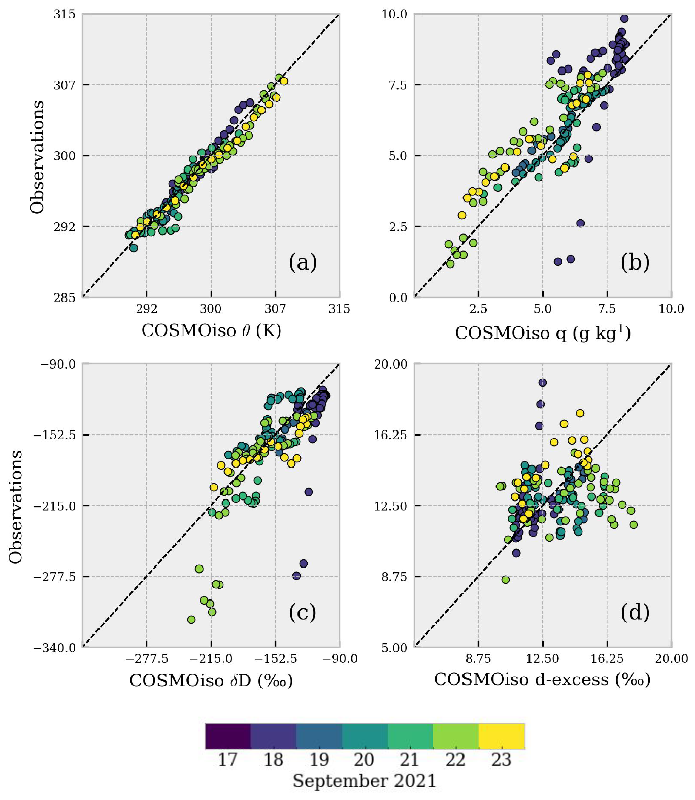
Figure 7 Comparison between COSMO_iso interpolated profiles and observations for the same variables of Fig. 6a–d. Dashed line represents a 1:1 relationship.

Potential temperature, q and δD simulated by COSMO_iso are in close agreement with observations for most of the flights as shown in Fig. 7 (r > 0.95 for 7 out of 12 flights, Fig. 6e–g). Noticeable differences between the model and observations are visible for flights on 18 and 22 September (blue and light green circles). The difference in δ values for 18 September flight can likely be attributed to the mismatch in simulated humidity: the COSMO_iso model simulates a more humid vertical profile above 2000 m, in terms of specific and relative humidity, which yields a more enriched water vapor in δ¹⁸O and δD at high-altitude levels. On the other hand, the difference in δ values for 22 September is not related to differences between simulated and observed humidity profiles. In general, COSMO_iso simulates a less depleted water vapor above 2500 $\mathrm{m}\mathrm{a}.\mathrm{s}.\mathrm{l}.$ for flights 7, 14 and 15, which are the flights where the largest δ¹⁸O and δD gradients were observed (such a bias is on average 10 ± 5 ‰ and 80 ± 37 ‰ for δ¹⁸O and δD, respectively). For the d-excess, the COSMO_iso model shows a similar or slightly higher variability than the observations which are relatively constant with height. A medium correlation (r > 0.5, p value < 0.01) was found between COSMO_iso and observed d-excess profiles for ∼ 50 % of the flights, but it is also worth noting that the direction of the correlation is negative for 3 out of 12 flights (5, 9, 10). Discrepancies between observed and modeled d-excess can be attributed to a weak correlation between observed and modeled RH profiles (r = 0.40) and to the influence of the land surface scheme and how this treats fractionation (Aemisegger et al., 2015).

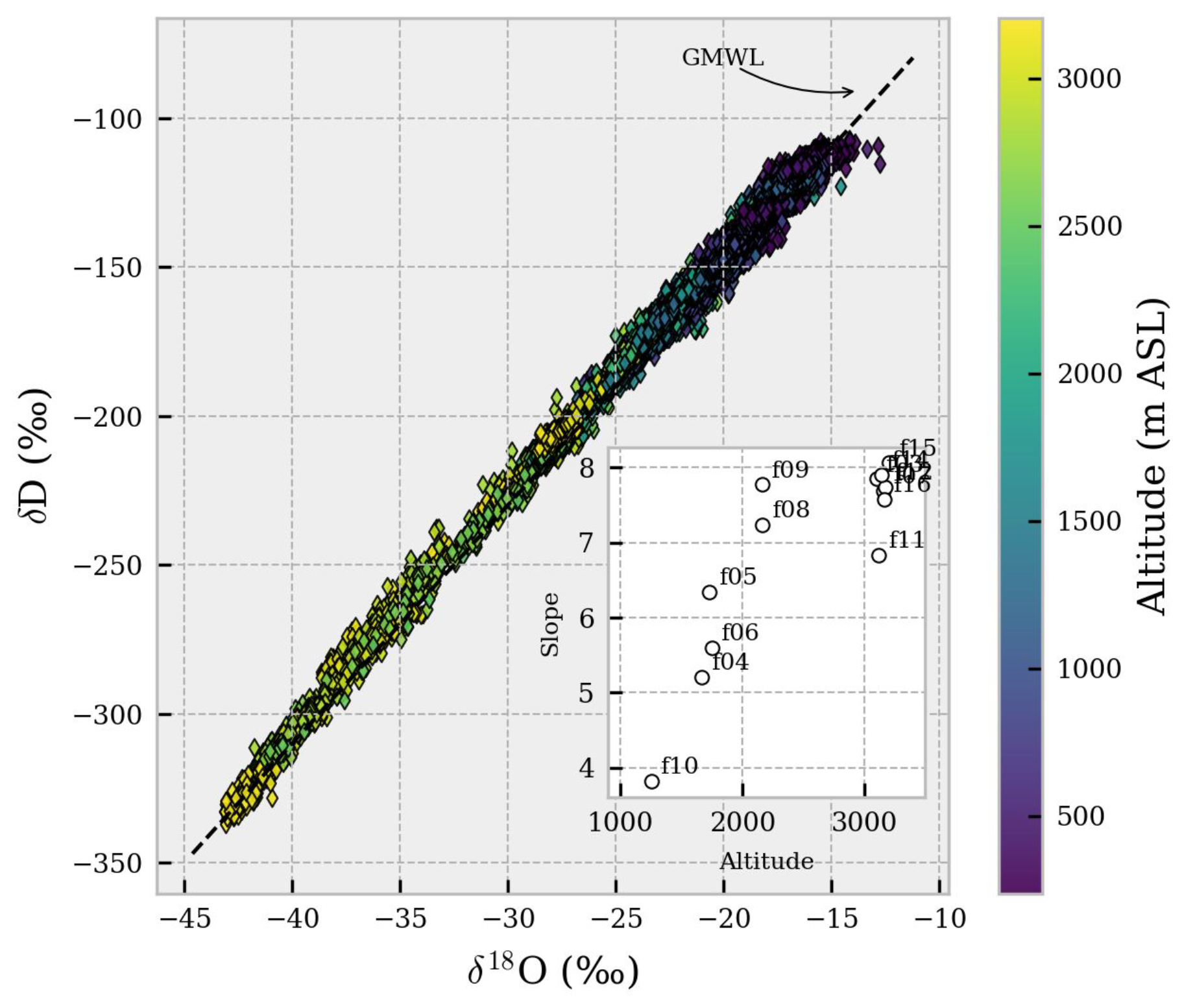
Figure 8 Distribution of the observations for all the flights on the δ¹⁸O vs. δD space. The GMWL (δD = 8 × δ¹⁸O + 10 ‰) is reported for reference. Inset plot: slope of the δ¹⁸O vs. δD (‰ ‰⁻¹) linear correlation for individual flights as a function of the maximum altitude (m) reached by each flight (r=0.84).

Table 2 Slopes of the δ¹⁸O vs. δD linear fit for individual flights (‰ ‰⁻¹). Flight extent below BLH reported as the percentage of data points collected below the BLH for each flight.

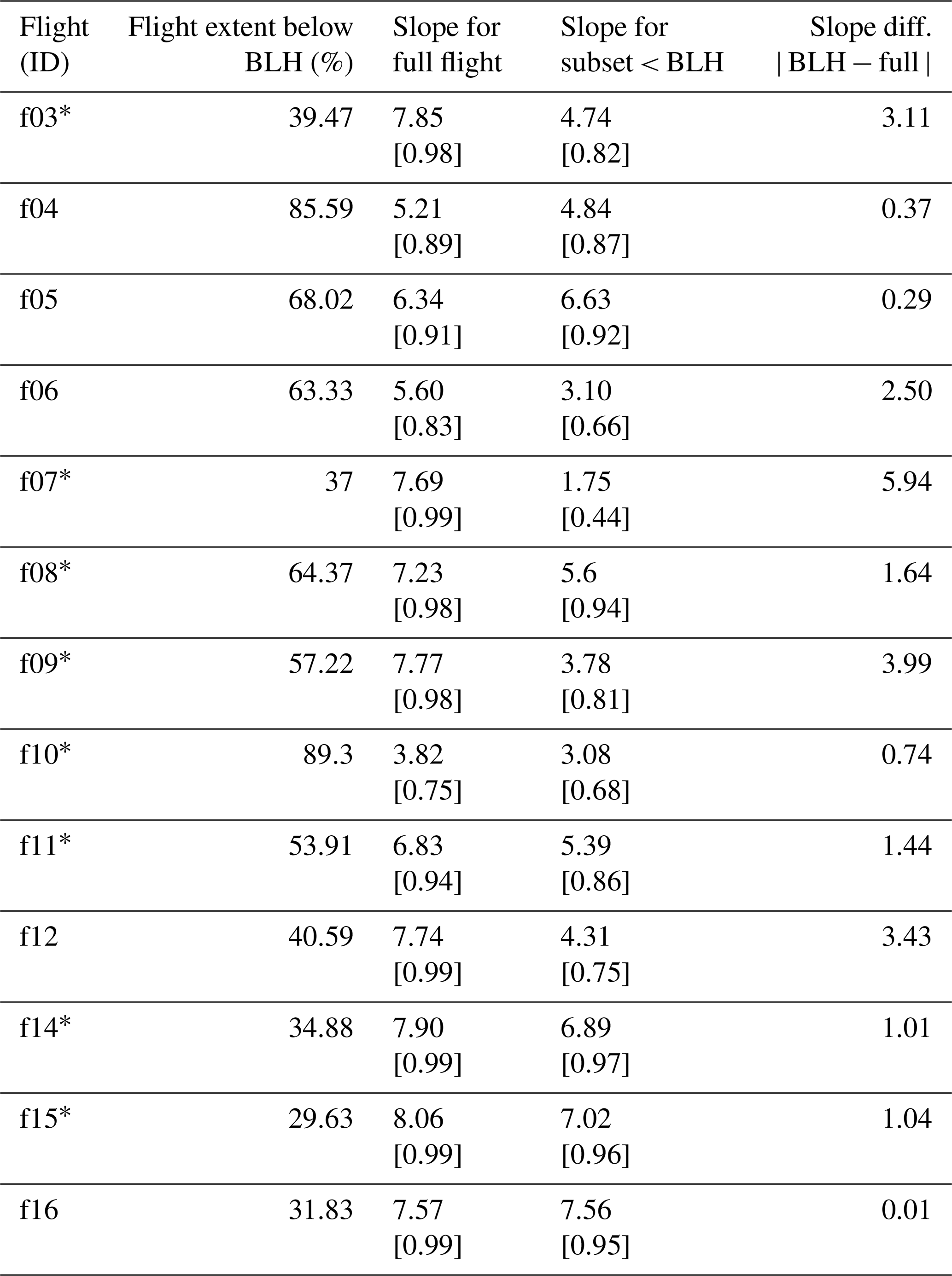
^∗ Denotes flights which flew over an area > 20 km². Correlations reported in brackets.

3.3 Water vapor δ¹⁸O vs. δD relationship in the lower troposphere: correlation with altitude and the impact of surface flux on boundary layer moisture

All the ULA flights crossed the boundary layer top (min, mean, max: 949, 1221, 1681 $\mathrm{m}\mathrm{a}.\mathrm{s}.\mathrm{l}.$, respectively). The observed water vapor isotopic composition retrieved from the ULA can therefore be considered representative of the water vapor within the boundary layer and can also provide insights about the water vapor composition of the lowest part of the free troposphere. When the δ¹⁸O and δD data points from all the flights are combined together, the regression becomes δD = (7.88 ± 0.003) × δ¹⁸O + (10.53 ± 0.07 ‰) (Fig. 7). This regression line matches closely to the Global Meteoric Water Line δD = 8 × δ¹⁸O + 10 ‰ (e.g., Rozanski et al., 1993). A similar meteoric water line of δD = (7.76 ± 0.005) × δ¹⁸O + (8.12 ± 0.09 ‰) is obtained with COSMO_iso interpolated data. A slope close to 8 suggests that the same main process is modulating the water vapor isotopic composition and the isotopic composition of global precipitation. However, the δ¹⁸O vs. δD slope for each flight ranges from 3.82 to 8.06, indicating that a simple distillation is not the sole process involved. The Fig. 8 inset indeed depicts an evident positive correlation (r = 0.84, p value < 0.01) between the maximum altitude reached by the ULA and the δ¹⁸O vs. δD slope. This positive correlation reflects the imprint of enriched water vapor in the boundary layer moisture. Given the undersaturated conditions during the flights and the typical Mediterranean vegetation of the study area, this enrichment can be attributed to the local evapotranspiration signal. The BLH was then used as a threshold, assuming water vapor being more influenced by the surface evaporation flux below the BLH. Table 2 reports evident differences between the δ¹⁸O vs. δD slopes calculated only within the boundary layer or for the full vertical extent of the flight. A slope value > 7 is always observed when the water vapor sampled below the BLH accounts for ⪅ 50 % of the flight observations, indicating that a δ¹⁸O vs. δD slope smaller than ∼ 7 is typical of water vapor sampled within the boundary layer, as observed in several ground-based studies (e.g., Aemisegger et al., 2014).

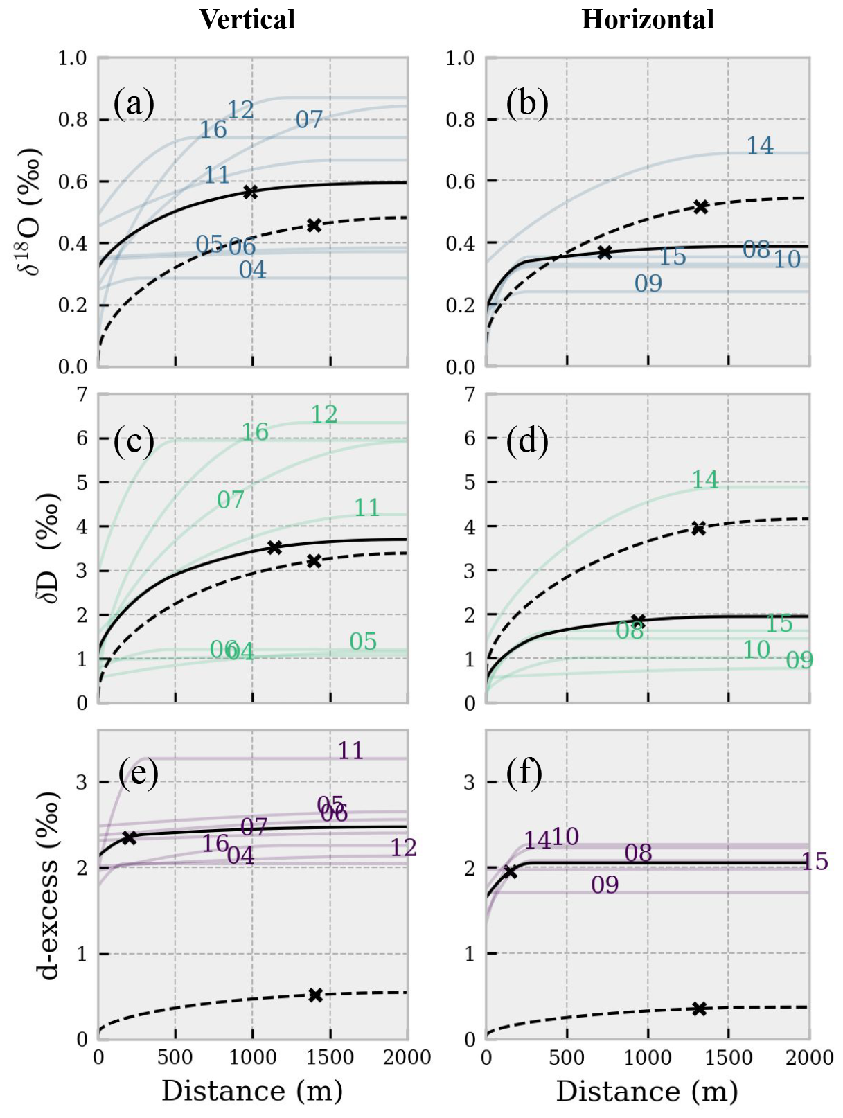
Figure 9 Square root of the semivariance of the δ vs. log(H₂O) model residuals as a function of the distance. δ¹⁸O (a, b); δD (c, d); d-excess (d, e). The colored lines represent the square root of the spherical model variograms estimated for each flight. Solid black lines are the ensemble means considering all the flights of the panel. Dashed black lines are the ensemble means calculated on COSMO_iso output interpolated on flight paths (variograms for each flight are not reported to improve visual interpretation). The “x” on the ensemble mean curves denotes the average distance at which residuals are uncorrelated (95 % of the sill).

Table 3 Span (max–min) and standard deviation of flights selected to probe the vertical and the horizontal variability of the water vapor isotopic signal.

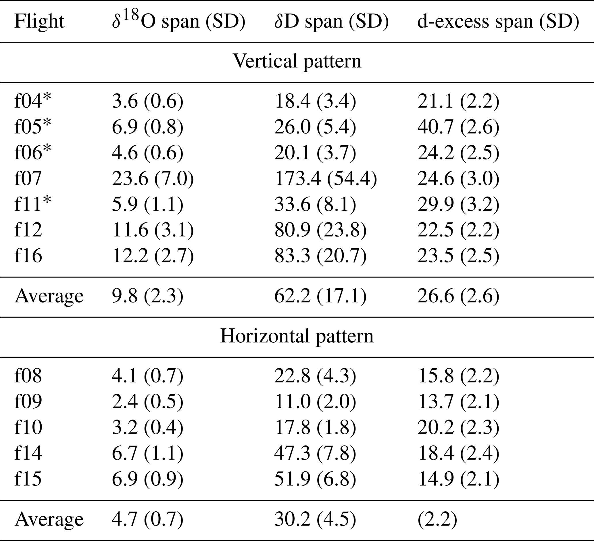
^∗ Denotes vertical profiles with number of observations within boundary layer > 50 %. All values in per mill (‰).

3.4 The vertical and horizontal variability of the isotopic composition of water vapor

Two types of flight patterns were used to investigate the 3D variability of water vapor isotopic signal in detail: vertical profiles (flights 4–7, 11, 12, 16) and horizontal scans (8–10, 14, 15). Specifically, flights 9 and 10 were designed to investigate the spatial variability at two and three different altitude levels, respectively. Flights 8–10 were performed over the hilly Aubenas area, while flights 14 and 15 were performed over the Rhône Valley, near the town of Montélimar. Figure 9 focuses on δD, as remote sensing techniques such as lidar and satellite instruments only target ${\mathrm{H}}_{\mathrm{2}}^{\mathrm{16}}\mathrm{O}$ and HD¹⁶O absorption bands, not ${\mathrm{H}}_{\mathrm{2}}^{\mathrm{18}}\mathrm{O}$. δ¹⁸O and d-excess maps are provided in Figs. S4 and S5 in the Supplement. The δ¹⁸O, δD and d-excess variability is discussed hereafter in terms of range (max–min) and of standard deviation (Table 3). The isotopic variability is larger in vertical profiles than in horizontal scans, consistent with expected temperature and humidity gradients. The vertical-to-horizontal range ratio is 2:1 for δ¹⁸O, δD and d-excess, while the vertical-to-horizontal standard deviation ratio is 3:1, 4:1 and 1:1, respectively, highlighting δD as the most sensitive parameter in both directions. The standard deviation correlates strongly with the flight extent for vertical flights (0.65, 0.66 and 0.40 for δ¹⁸O, δD and d-excess, respectively), meaning that a wider range of δ¹⁸O and δD values were observed as the ULA traversed a larger vertical extent. Horizontal scans show a similar correlation for δ¹⁸O and δD with flown-over area but not for d-excess. Similar to other studies, this dataset also shows a good correlation between the water vapor isotopic composition (δ¹⁸O and δD) and the logarithm of the specific humidity, allowing a linear regression model with log(q) as the sole predictor to explain over 90 % of δD variability in vertical flights. Notably, for flight 7, a high-altitude sounding, log(q) can explain over 99 % of the δD variability. For horizontal scans, the explained variance is smaller but still high on average ($r_{\mathit{\delta }\mathrm{D}}^{\mathrm{2}}$ vs. q=0.74; see Table S2 in the Supplement reporting all the r² values). While COSMO_iso reproduces observed vertical δ−log(q) patterns, best-fit parameters differ between horizontal and vertical flights in model simulation. Indeed, observed δD vs. log(q) slopes average are very similar at 69.4 and 68.9 for vertical and horizontal flights, whereas COSMO_iso estimates 65.8 and 122.2, respectively.

3.5 The vertical and horizontal spatial structure of the isotopic composition of water vapor

Determining the spatial correlation of water vapor isotopes helps optimize the interpolation of sparse observations and assess the ability of CRDS technology to detect fine-scale atmospheric processes using fast-moving airborne observations like from ULA. However, given that water vapor isotopic composition is strongly correlated with the specific humidity (and consequently with air temperature), here we explore the variogram of the residuals of the linear model defined between log(q) and δ values. This approach enabled the investigation of the spatial correlation of different isotopologues of water vapor alone. The variograms for δ¹⁸O, δD and d-excess for both flight patterns are shown in Fig. 9. A spherical model was used to fit the observed semivariance within a maximum lag distance of 5 km. The same procedure was applied to COSMO_iso output. Even though each flight presents a specific pattern, some general observations can be made. First, a large part of the variance in isotopes can be explained by the variability of the specific humidity, and the average variability of model residuals is only ∼ 0.5 ‰, ∼ 2.8 ‰ and ∼ 2.3 ‰ for δ¹⁸O, δD and d-excess, respectively (the sill values for observations in Fig. 9). Such values are only slightly larger than instrumental precision and must therefore be interpreted carefully. In this context, it is clearly visible that the average variograms computed on observations and those from COSMO_iso output are offset by ∼ 0.3 ‰, ∼ 1 ‰ and ∼ 2 ‰ at 0 m distance (i.e., the nugget values), consistent with the values attributed to instrumental uncertainty (0.23 ‰, 0.50 ‰ and 1.78 ‰ for δ¹⁸O, δD and d-excess, respectively). Secondly, the spatial structure extrapolated from observations differs between vertical and horizontal flights. This spatial anisotropy is especially noticeable for δD, as highlighted in Sect. 3.4, and the COSMO_iso model seems to not capture such anisotropy. Finally, the spatial correlation of the model residuals acts over a short range, averaging ∼ 1000 m for both δ¹⁸O and δD in observations. The key takeaway is that beyond such a distance, the isotopic composition of water vapor becomes largely independent of spatial separation, with most of its variability being driven by changes in humidity. For d-excess, the range is limited to less than 250 m in observations and ∼ 1300 m in COSMO_iso. Given such a limited variability, it is not possible to formulate more detailed hypotheses about d-excess.

Focusing on the observations, the vertical variograms in Fig. 9 show a striking difference between low-altitude and high-altitude flights (flights 4, 5, and 6 and flights 7, 11, 12 and 16). Hence, the spatial correlations for vertically resolved observations of water vapor isotopic composition are stronger the larger the atmospheric column probed is. This is reasonable, since different height levels can be representative of different large-scale circulation and therefore can be imprinted by water vapor with different isotopic signatures. Flight 10 provides insights on how the spatial pattern of water vapor isotopic composition is sensitive to the fine-scale (< 100 m) process, as further discussed in Sect. 3.6. For horizontal flights on single levels, all the flights but fight 14 show a similar pattern in spatial structure. As can be noted from Fig. 1, flight 15 is almost a replica of flight 14 in terms of flight pattern, location and altitude level. However, flight 14 was performed in the morning and flight 15 in the early afternoon. The key differences between these two flights are further discussed in Sect. 3.7.

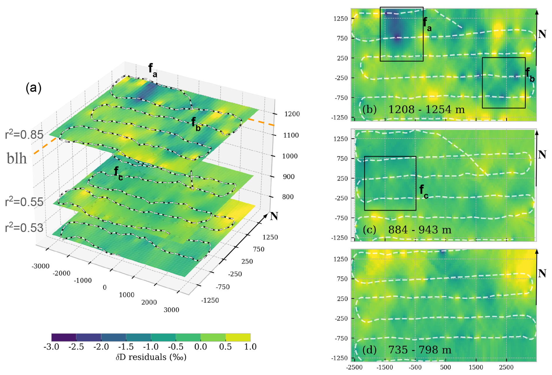
Figure 10 Residual field of the δD vs. log(q) model at different altitudes during flight 10 obtained by ordinary kriging. (a) Stacked view of levels L1200, L900 and L700 at average altitude level (1229, 917 and 763 $\mathrm{m}\mathrm{a}.\mathrm{s}.\mathrm{l}.$). The orange dashed line indicates the boundary layer altitude (1120 $\mathrm{m}\mathrm{a}.\mathrm{s}.\mathrm{l}.$). (b–d) Details of residual fields for each level. The text reports the min–max altitude recorded by ULA for that level. For all panels, the zebra-style lines indicate the ULA path. Areas marked with f_x are discussed in the text. All axis values in meters (the arrow points to the geographical north). For panel (a) vertical exaggeration is ∼ 9 to emphasize vertical features.

3.6 Detection of water vapor isotope spatial structures at different altitudes in the boundary layer

Now we analyze the fine-scale horizontal structures in the variations of the stable isotope composition across different levels of the boundary layer targeted during specific flights. The second part of flight 10 consisted in the spatial sampling of the atmosphere at three different altitudes in the boundary layer near the Aubenas Aerodrome: 763 ± 12 m, 917 ± 13 m and 1229 ± 8 m, hereafter L700, L900 and L1200 (Fig. 10a). Each level was probed for 20–30 min and covered a horizontal scale of 6.1 km × 2.8 km. A well-mixed atmosphere and low variability of δD can be observed within the boundary layer, as shown in Fig. 10c and d. The small-scale variability of δD and q is reflected by the low r² for the δD vs. log(q) regression model of individual horizontal scans at L700 and L900 (0.53 and 0.55, respectively).

At L1200, close to the boundary layer height, the r² significantly increases (0.83) and the spatial features in the residual field are more evident (Fig. 10b). While the q variability remains similar across levels (∼ 0.1 g kg⁻¹), the slightly larger δD variability at L1200 (3 ‰ vs. 1 ‰) can be attributed to the short-range exchange of water vapor with different isotopic signatures between the boundary layer and the free atmosphere. The non-random spatial structure of residuals is confirmed by Moran's I, which is statistically significant for all the three altitude levels, and it is the highest for the top level (Moran's I =0.44, p value < 0.01, estimated with a distance band of 250 m). More specifically, the features f_a and f_b highlight short-lived and size-limited processes that are characterized by more depleted water vapor than predicted by the δD vs. log(q) relationship. These coherent features are not related to water vapor analyzer performances, since no correlation was observed between model residuals and instrument performance indicators such as sudden changes in cavity temperature or cavity pressure, proving that these features are measurable changes in the water vapor isotopic composition. Additional proof of the presence of such spatial features is given by the fact that each feature is probed by the ULA at least twice, in the opposite cruise direction. Interestingly, there is no apparent direct link between spatial features at the different levels observed. For instance, feature f_c on L900 cannot be easily associated with feature f_a on L1200, meaning that such features are highly resolved on the vertical axis and distributed over the horizontal plane on the order of ∼ 1 km. Therefore, we speculate that the ULA may have captured intermittent coherent structures which are commonly observed at the boundary layer top over terrain with high surface roughness (Thomas and Foken, 2007), while residual fields for horizontal scans within the lowermost layers are mostly driven by instrumental uncertainty (∼ 1 ‰ for δD).

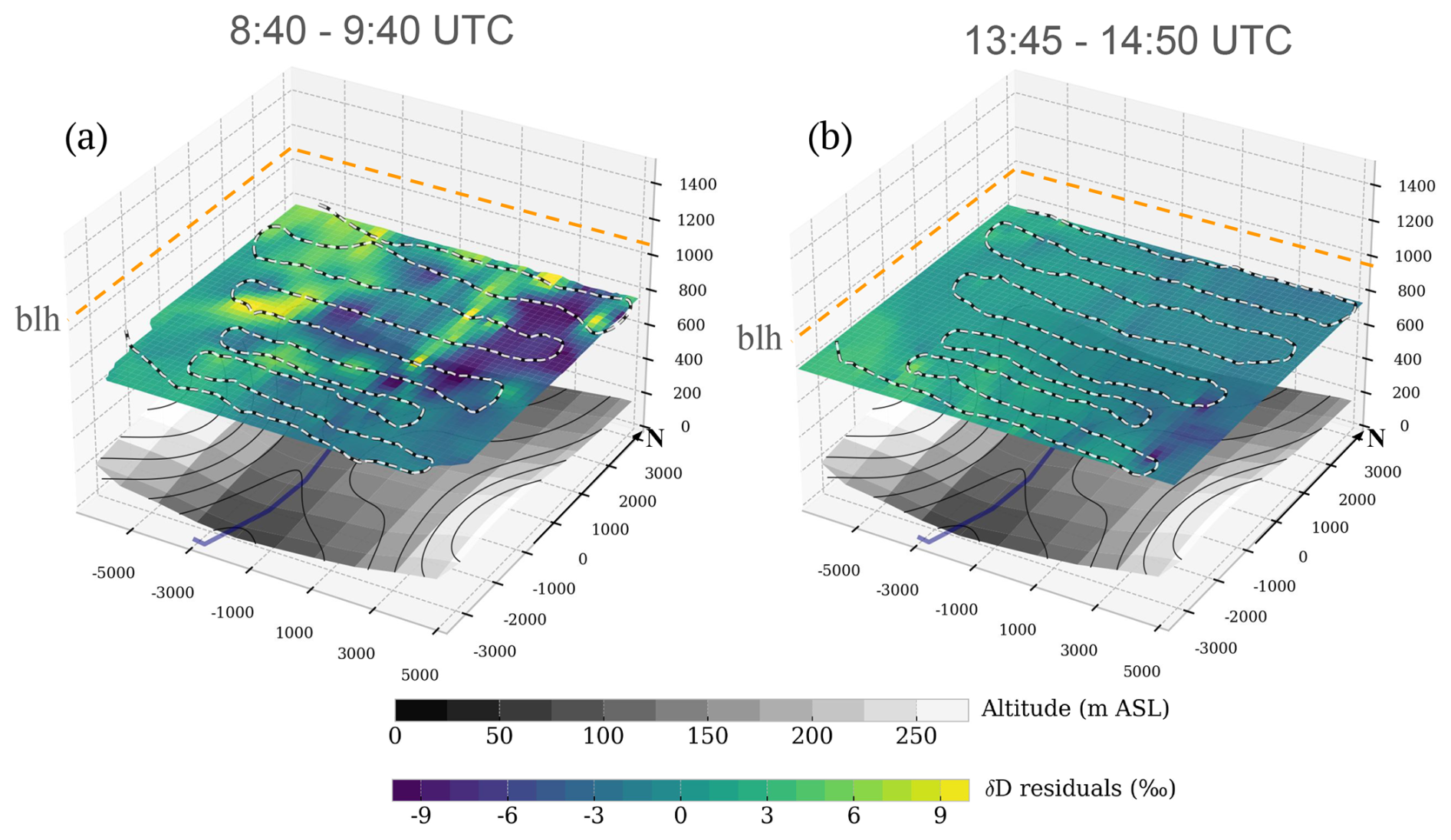
Figure 11 Residual field of the δD vs. log(q) model obtained by ordinary kriging for the same location above the Rhône Valley at different times of the day: (a) morning flight 14 and (b) afternoon flight 15. Color, unit and line format like Fig. 10. Underlying topography and the Rhône River are reported for reference. All axis values in meters (the arrow points to the geographical north). For altitude, the vertical exaggeration is ∼ 5 to emphasize vertical features.

3.7 Temporal evolution of water vapor isotope spatial structures throughout the day

Flights 14 and 15 were designed to probe the spatial variability of water vapor isotopic composition above the Rhône Valley at different times during the day, as shown in Fig. 11. Notably, flights 14 and 15 are characterized by large spatial autocorrelation (Moran's I = 0.87 and 0.72), but flight 14 is characterized by the strongest spatial autocorrelation structure among all the horizontal pattern flights (see Fig. 9).

A few hours later, flight 15 shows that the same area is characterized by a less evident spatial structure, and a larger r² of the δD vs. log(q) model can be observed with respect to flight 14 (0.53 vs. 0.90). As briefly shown on the three layers of flight 10, the more evident the spatial features in the residual fields are, the smaller the r². Following the underlying topography, it is possible to see that the simple specific humidity estimate reveals larger positive deviations on the west side of the map, where the morning sun very likely caused uneven heating of the Rhône Valley, promoting the formation of a thermal on the east-exposed slopes and enhancing the influence of enriched surface evaporation on the isotopic composition of atmospheric water vapor. In summary, the variability in the residual field is linked to early-stage boundary layer development during flight 14, while for flight 15, it reflects a well-mixed boundary layer state.

3.8 Application of a simplified conceptual model for simulating the vertical variability of water vapor isotopic composition

Having seen that the water vapor mixing ratio can provide a first-order approximation of the vertical and horizontal water vapor isotopic structure in the atmosphere, we will see here how conceptual models, based on humidity only, would deviate from expectation in terms of water vapor isotopic composition. As described for the observational data in Sect. 3.2, the specific humidity, water vapor isotopic composition and air temperature were binned and averaged over 20 height levels with 150 m vertical resolution for each flight. The squared difference (error) between modeled δ¹⁸O, δD, and d-excess and the bin-averaged observations was used as a metric to evaluate the performance of the conceptual models.

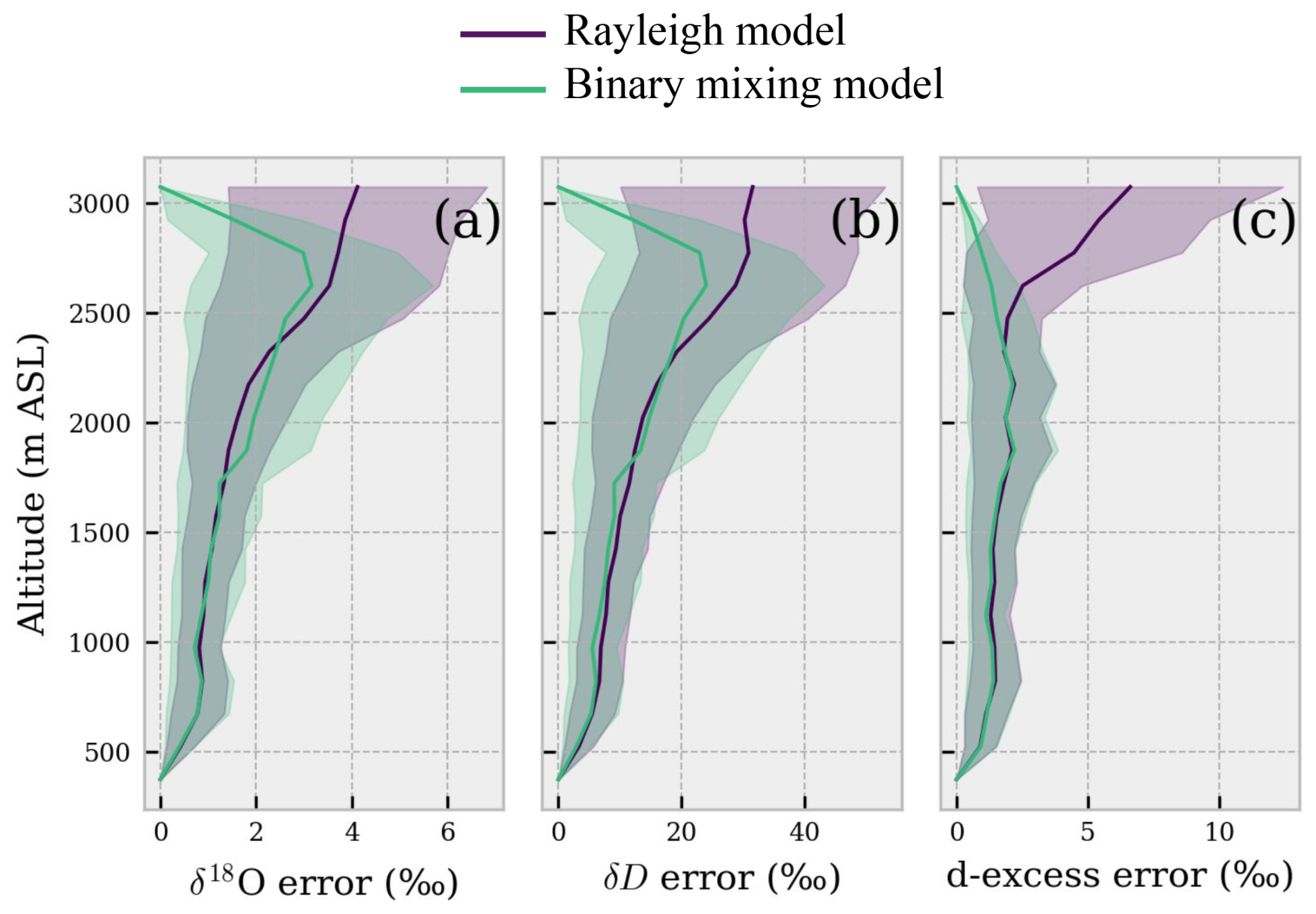
Figure 12 Root mean squared error (RMSE) between models and observations averaged per height levels for δ¹⁸O (a), δD (b) and d-excess (c). The solid lines represent the average error calculated over a 150 m bin size for all the flights, and shadings represent the standard error of the mean.

In general, both models can predict the variability of water vapor isotopic composition to a reasonable degree, as shown in Fig. 12. The actual modeled vertical profiles compared to observations are available in Fig. S6a–c in the Supplement. Globally, considering all flights and vertical levels, the root mean squared error (RMSE) varies within narrow ranges: [1.5–1.8] ‰ for δ¹⁸O, [11–15] ‰ for δD and [1–2] ‰ for d-excess. Both conceptual models achieved very similar results within the boundary layer (< 1000 $\mathrm{m}\mathrm{a}.\mathrm{s}.\mathrm{l}.$). However, it is worth noting that even though both models produce similar results, the Rayleigh model is in principle less suited to explain the processes of a strongly mixed and turbulent boundary layer, where there is water vapor mixing between the free troposphere and surface evaporation flux, as suggested, e.g., in Benetti et al. (2018) for marine environment. This hypothesis is partially supported by the fact that the binary mixing model generally performed better than the Rayleigh model. Indeed, the Rayleigh model should be better suited to describe the development of a convective cloud, which was not the case for most of the flights in this study except for flight 11, which was specifically designed for sampling water vapor above and below (but not within) a convective cloud. Nevertheless, results show that water vapor isotopic observations measured above 2500 m are challenging to capture for both the Rayleigh and mixing models, as both methods yield large errors for δ¹⁸O and δD. Similar results are obtained using COSMO_iso as reported in Fig. S7 in the Supplement. The mixing model performs better than the Rayleigh model in simulating d-excess, although the differences between the two models are small. The mixing model shows a smaller RMSE (∼ 1 ‰) and a d-excess error distribution that is consistent across different height levels. Further, the error for the Rayleigh model is more spread out above 2000 $\mathrm{m}\mathrm{a}.\mathrm{s}.\mathrm{l}.$. The analysis of d-excess profiles for individual flights reveals that the shape of Rayleigh-simulated profiles is almost flat below 2500 $\mathrm{m}\mathrm{a}.\mathrm{s}.\mathrm{l}.$ (not shown), which is expected because d-excess variability is small during equilibrium fractionation in the Rayleigh distillation process. The d-excess simulated with the mixing model follows the general trend of observed d-excess within the vertical profile.

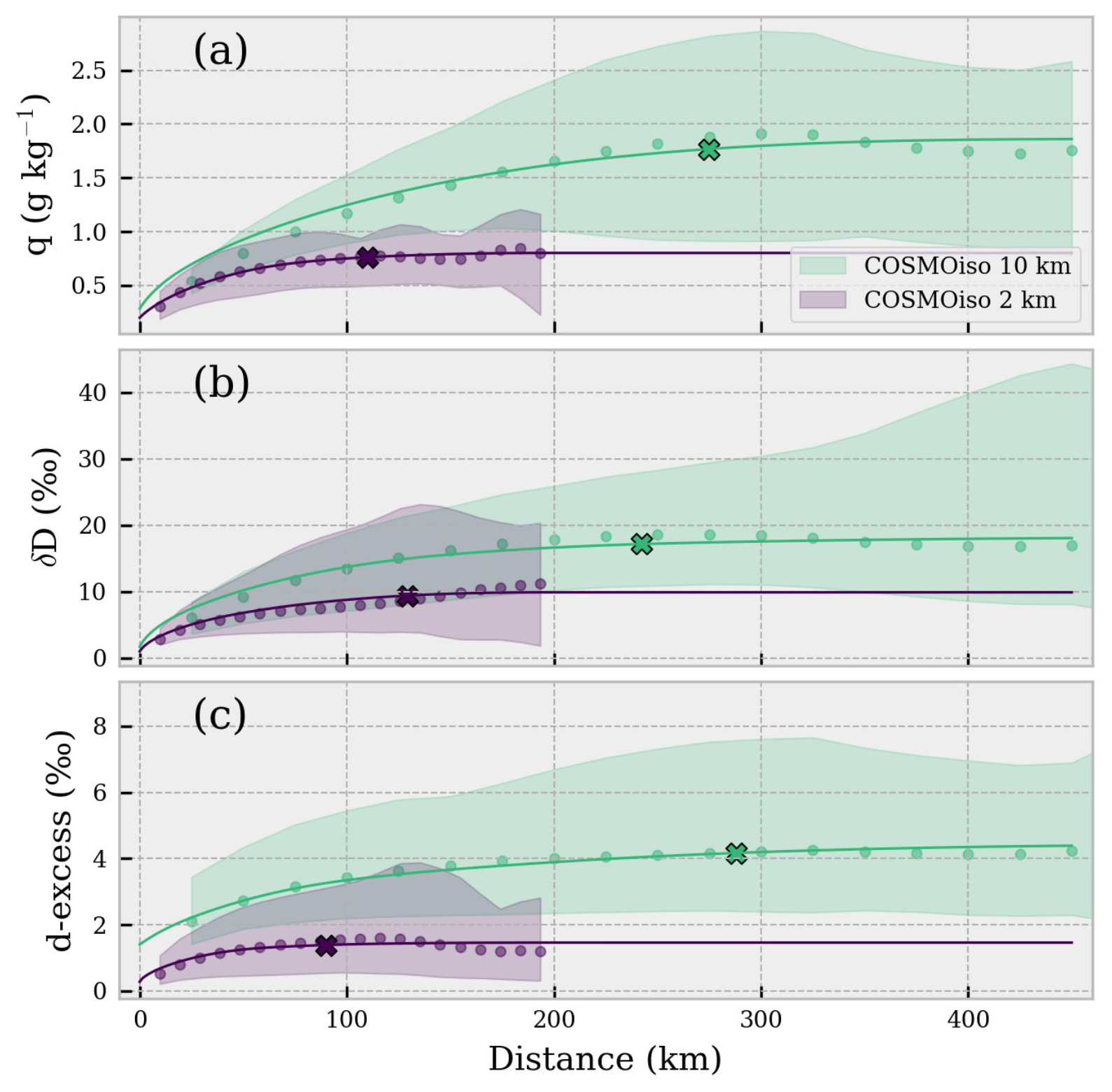
Figure 13 Similar to Fig. 9, the square root of the semivariance of q, δD and d-excess (a–c, respectively) in the COSMO_iso model. For all panels, colors are representative of model runs at different resolutions, dots are the average experimental variogram, and solid lines and shadings represent the ensemble mean and min–max interval of the square root of the spherical model variogram. The “x” on the ensemble mean curves denotes the average distance at which residuals are uncorrelated (95 % of the sill).

4 Discussion

4.1 Spatial representativeness: at what distance are water vapor isotope observations statistically independent?

As shown here and in several other studies, the log of specific humidity and the water vapor isotopic composition are strongly correlated (e.g., Lee et al., 2007; Sodemann et al., 2017). Therefore, the spatial representativity of water vapor isotope observations is intrinsically related to the spatial representativeness of water vapor mixing ratio to a first order (if dominated by turbulent mixing). The spatial correlation scale of the atmospheric water vapor is a quantity that depends on the turbulence conditions of the atmosphere and on the weather regime among other factors. Therefore, the spatial representativeness of specific humidity can exhibit patterns across different spatial and temporal scales. In this study we observed that the semivariance of specific humidity at a given spatial separation estimated from horizontal pattern flights at different altitudes tends to continuously increase as a function of the distance, and no observable plateau can be identified within a radius of 5000 m (see Fig. S8 in the Supplement). Hence, the 2 and 10 km resolution COSMO_iso lowest level data were used to replicate a similar analysis on a large area (3° × 4°) centered over Aubenas. The results in Fig. 13a, extrapolated at the same time of the flights, reveal the occurrence of one or more plateaus for specific humidity at different separation distances, depending on the model resolution. As a further control, the same analysis was performed on the specific humidity of ERA5 at the lowest pressure level, confirming that a first plateau can be identified between 100–300 km, varying from day to day (data not shown). The results reported in this study agree with the findings by Park et al. (2018) which report a drop in spatial correlation for water vapor concentration at a separation distance > 100 km. As expected, similar results in term of separation distance and drop in spatial correlation are obtained for δ values and d-excess (Fig. 13b and c; the observed semivariance pattern in this study is similar for δ¹⁸O and δD and is not reported here). A similar separation distance (300 km) has also been used by Thurnherr et al. (2024) to obtain total-column-averaged δD retrievals from the S5P satellite in southern France. In conclusion, 100 km can be considered an approximate threshold for collecting statistically independent water vapor isotope observations when considering processes acting on the mesoscale.

4.2 Stable isotopes of water vapor highlight fine-scale processes and coherent structures of the water vapor field: current limits using CRDS analyzers

When the covariance between the humidity and its isotopic composition is accounted for through simple linear regression or by means of conceptual models, fine-scale processes can be detected by fast and localized changes in the isotopic composition of water vapor alone. The example of flight 10 shown in Sect. 3.6 highlights how localized fine structures in the 3D isotopic composition water vapor field are. Spatial autocorrelation of δ vs. log(H2O) model residuals drops rather quickly, and, considering the features identified in Fig. 10, such intermittent coherent structures in the water vapor stable isotope field can be approximated to a spheroid with a horizontal radius ∼ 500–1000 m and vertical radius ∼ 150 m in the boundary layer. In a very simplistic approach, considering horizontal wind speed on the order of 3–5 m s⁻¹ the lifetime of such structures is on the order of 100–300 s, which is well below the response time of the CRDS analyzer. However, the lifetime of water vapor coherent structures has been reported to vary over a wide range, and their occurrence can change throughout the day (see, e.g., Tyagi and Satyanarayana, 2014; Dias-Júnior et al., 2013). Hence, spatial autocorrelation can change quickly as a function of time depending on changes in wind speed, thermodynamic conditions and stability within the boundary layer. For instance, flight 14 and 15 in Sect. 3.6 showed that differential heating due to topography, likely introducing the development of thermals, can produce significant changes in the water vapor stable isotope field. Our results demonstrate that water vapor isotopes are a valuable tool for investigating boundary layer development, turbulent mixing processes, and the influence of coherent structures on the exchange between the boundary layer and the free troposphere. The high instrumental precision and acquisition rate enable the detection of short-lived turbulence-related processes with sufficient accuracy. However, technical issues might arise when studying such water vapor isotopic composition structures at a higher frequency, due to the slow response time and the memory effect in current CRDS measurement technology. Thus, optimal filtering of isotopic signals as proposed in Sect. 2.4 is paramount and has been used for a fixed two-level keeling plot with a roughly hourly timescale to accurately determine the isotopic composition of the ocean evaporation flux (Steen-Larsen et al., 2014; Zannoni et al., 2022) and evapotranspiration (Aemisegger et al., 2014). Further corrections are indeed necessary when fluxes are estimated at an even higher frequency, such as with eddy covariance–CRDS coupled systems (Wahl et al., 2021). The recent work by Meyer and Welp (2024) highlights that flow rate and optical cavity volume are indeed key factors contributing to the overall memory effect in laser analyzers. In addition to this, we suggest using a short, low-memory inlet material (e.g., polished or coated stainless steel, copper), suitable heating or insulation, and fast flow rates when performing high-frequency measurements. We also emphasize the need for a dedicated study to identify the best materials and optimized high-flow-rate settings for water vapor isotope flux analysis, which would greatly benefit the isotope-hydrology community.

4.3 Vertical representativeness: to what extent do surface observations reflect water vapor isotopic composition in the atmospheric column? Toward a tentative extrapolation of δD

The results of this study depict a limited variability in water vapor isotopic composition in the horizontal space and a large variability in the vertical direction. Such a variability accounts roughly for a 1:4 ratio, based on δD standard deviations, which might be sensitive to measurement uncertainty and to the shape of the isotope data distributions. As mentioned before, the large vertical variability is not surprising given the large temperature and humidity gradients in the atmospheric column. However, the results of the comparison between the conceptual models and ULA observations suggest that a few data points within the boundary layer can be used to estimate the vertical profile of the water vapor isotopic composition up to several kilometers with a certain degree of confidence. Despite the results in Sect. 3.4 indicating vertical turbulent mixing as the main controlling process of the water vapor isotopic composition in the lower troposphere, the quantities involved in such idealized two-end-member models are not straightforward to predict. Most important, information about the average water vapor isotopic composition of the free atmosphere (δ₀) and information about the isotopic composition of the surface flux (δ_F) are required terms in the mixing equation. For example, we estimated a change from δ¹⁸O_F = −6.12 ‰ at 05:00 UTC to δ¹⁸O_F = −13.38 ‰ at 15:00 UTC on 18 September (flights 4 to 7) with the keeling-plot method applied on 150 m binned vertical profiles. Intriguingly, the average δ¹⁸O of water vapor in isotopic equilibrium with precipitation for September 2021, estimated from altitude-corrected GNIP (IAEA) data and air temperature records from Avignon (∼ 100 km south, ECA&D), is −13.38 ‰. Although this estimate assumes saturation and equilibrium, making it approximate, it supports the hypothesis that evapotranspiration influences boundary layer moisture during the day. However, the observed shift in the δ¹⁸O_F end-member composition from morning to afternoon also indicates that assigning a constant isotopic signature based on nearby precipitation is not reliable. The same applies for the variability of the dry end member δ₀, whose composition can only be guessed or measured with dedicated high-altitude flights. However, it should be noted that the results showed the δD vs. log(q) relationship holding even if the controlling physical process modulating the isotopic composition in the lower troposphere is mixing, which in principle should be represented by a hyperbole in the q–δ space (the reader is referred to Fig. S9 in the Supplement for a comparison among observations, Rayleigh distillation and mixing model). Mathematically this can be explained by the fact that a hyperbolic curve can be fitted by a logarithmic curve within a limited range of values.

Focusing on δD, which can be also retrieved with remote sensing through the atmosphere, the best-fit parameters of the log-linear model δD = ${\mathit{\beta }}_{\mathrm{0}}\times \text{log}\left(q\right)+{\mathit{\beta }}_{\mathrm{1}}$ [‰] for all the flights of this study are β₀ = 93.86 and β₁ = −324.0 (see Table S3a and b in the Supplement for individual best-fit parameters of each flight). It is worth noting that the shape of the δD vs. q relationship is similar across different airborne datasets, as shown in Fig. 14 (Chazette et al., 2021; Dyroff et al., 2015; Dyroff et al., 2021; Salmon et al., 2019; Schneider et al., 2015; Schneider et al., 2018; Sodemann et al., 2017; Wei et al., 2019). Figure S10 in the Supplement shows the resulting plot on a semi-log space.

Indeed, β₀ shows small variability, ranging from 70.62 (Annecy, Chazette et al., 2021) to 103.96 (Indianapolis, Salmon et al., 2019). When all the observations are combined β₀ = 72.31 ± 0.94, where the uncertainty is the standard error of the slope. Similarly, the β₁ parameter ranges from −324.0 to −243.1 (yielding β₁ = −269.4 ± 1.6 for all combined observations). Such a limited variability in the best-fit parameters highlights that the log-linear approximation of the mixing process holds its shape across different locations and for different vertical extents of the tropospheric column probed with each flight. Changes in the weather conditions, such as strong/weak convection, strong/weak entrainment, atmospheric stratification, and presence of clouds, are likely to affect the shape parameter (β₀). Changes in the isotopic composition of the two end members of the binary mixing (i.e., the water vapor in the boundary layer and in the free troposphere) are likely to affect the intercept parameter (β₁).

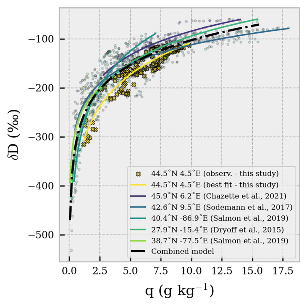
Figure 14 δD vs. q over 150 m binned vertical profiles estimated for different airborne campaigns. The legend reports the coordinates of the flights and the reference study. Symbols are observations; solid lines are best-fit curves. The black dot-dashed line is the best-fit curve combining all the binned vertical profiles from all the datasets. The best-fit model for all the curves is δD = ${\mathit{\beta }}_{\mathrm{0}}\times \text{log}\left(q\right)+{\mathit{\beta }}_{\mathrm{1}}$.

The main advantage of such a log-linear approximation is that just a single-level observation of δD and the tropospheric humidity profile are necessary to produce an approximation of the tropospheric profile of water vapor δD in clear-sky conditions. This in turn can be used to estimate the weighted average water vapor column δD, providing information on the total column water vapor δD (assuming the measured humidity profile captures ∼ 100 % of the total column water vapor). Following this approach, the single-level observation can be surface observations of water vapor isotopic composition that are representative of the boundary layer. The vertical distribution of the water vapor mixing ratio can be retrieved with regular vertical profiling such as radiosounding. To scale the log-linear model for a specific location and time, the model can be rearranged in the form

$$\begin{array}{}\text{(2)}& \mathit{\delta }\mathrm{D}={\mathit{\beta }}_{\mathrm{0}}\text{log}\left({\displaystyle \frac{q}{q_{\text{SURF}}}}\right)+{\mathit{\delta }\mathrm{D}}_{\text{SURF}},\end{array}$$

where β₀ is the best-fit parameter reported above (72.31 ± 0.94), q is the specific humidity profile [g kg⁻¹], q_SURF is the mixing ratio measured at the surface [g kg⁻¹] and δD_SURF is the water vapor δD measured at the surface. Figure 15 shows the distribution of the differences between modeled and observed weighted average water vapor column δD considering all the datasets used to generate Fig. 4. The mean difference between observed and modeled weighted average δD is 4.2 ± 12.7 ‰ (n = 59). However, when considering only flights which probed the troposphere for a vertical extent of at least 5000 $\mathrm{m}\mathrm{a}.\mathrm{s}.\mathrm{l}.$, the difference becomes 12.2 ± 6.7 ‰ (n = 6, all flights from Dyroff et al., 2015). On average, the log-linear model returns negatively biased δD values. The root mean squared error between observed and modeled weighted average δD can be representative of the uncertainty of the log-linear model approximation, being also very similar when using all the datasets and when using only datasets with flights > 5000 $\mathrm{m}\mathrm{a}.\mathrm{s}.\mathrm{l}.$ (13 ‰ and 14 ‰, respectively). It is worth noting that with the simple generalization of the log-linear model important processes such as advection and cloud formation can be easily missed. Hence, model extrapolations should be approached with caution, and a clearer understanding of the factors influencing the β₀ and β₁ parameters is essential to provide an initial approximation of the δD profile for potential satellite validation. It is important to note that the analysis presented in this section focuses on a limited latitudinal range, specifically the mid-latitudes (38–46° N), with only a few data points from the subtropics (Dyroff et al., 2015). Consequently, the findings reported here may not be directly applicable to equatorial or polar regions. Additionally, most of the studies included in this analysis were conducted over continental areas, with the exceptions of Sodemann et al. (2017) and Dyroff et al. (2015), which include observations over the Mediterranean Sea (Corsica) and the Atlantic Ocean (Tenerife), respectively. The impact of different weather regimes must also be considered, as data collection during aircraft campaigns is typically constrained by flight safety conditions. As a result, observations during periods of strong updrafts, convection or intense winds are unlikely to be available. In fact, all the flights analyzed in this study were conducted under mostly clear-sky conditions, with minimal cloud presence and low convection. An exception is found in Salmon et al. (2019) and Dyroff et al. (2015), where one flight of the former study was carried out in the presence of large stratocumulus clouds and an inversion layer just below the cloud base and one flight of the latter study was performed with haze conditions during a Saharan dust transport event. It is worth noting that in Salmon et al. (2019), that specific flight case was used to investigate how a stratocumulus cloud layer can influence the isotopic composition of water vapor in the lower stratosphere, similarly to flight 11 in this study. Furthermore, this study and Sodemann et al. (2017), Dyroff et al. (2015) and Chazette et al. (2021) were all conducted under the presence of strong high-pressure systems, characterized by large-scale subsidence. Additionally, the flights analyzed in Chazette et al. (2021) were performed over a large lake in a valley, where the strong influence of lake moisture on the boundary layer can be observed as a significantly different δD vs. log(q) relationship compared to this study (see the purple vs. yellow lines in Fig. 14). This discrepancy occurred despite the geographical distance, similar latitude, comparable weather conditions and the same time of year (∼ summer). Despite these limitations, this exploratory analysis highlights the value of incorporating the stable isotopic composition of water vapor to improve the parameterization of atmospheric hydrological processes. This approach may offer more accurate insights than relying solely on variations in specific humidity, as demonstrated by numerical weather forecast simulations (Yoshimura et al., 2014; Toride et al., 2021).

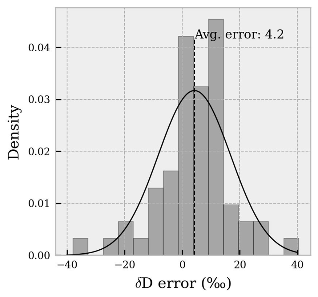
Figure 15 Error distribution (observed – modeled) of the estimated weighted average atmospheric δD. The solid black line represents a normal distribution with mean = 4.2 ‰ and standard deviation = 12.7 ‰.

5 Conclusions

In this study, we used a highly temporal and spatially resolved airborne dataset in combination with conceptual and numerical models (COSMO_iso) to gain insights into the controlling factors of water vapor isotopic composition in the lower troposphere and its spatiotemporal representativeness. Our findings indicate that vertical mixing is the dominant process affecting isotopic variability in the lower troposphere at hourly and sub-daily scales for this study. Within such a temporal scale, significant isotopic fractionation effects, as well as possible advection, become important at altitudes above 3000 m. At these higher altitudes, both conceptual and numerical models struggle to accurately simulate water vapor isotopic composition. Interestingly, our flights' combined data perfectly align with the Global Meteoric Water Line (GMWL), unlike typical surface-only studies which often report δD vs. δ¹⁸O slopes smaller than 8. However, the δD vs. δ¹⁸O slope varied by flight, showing a strong positive correlation between the maximum altitude reached by each flight and the slope. Small slope values (< 8 ‰ ‰⁻¹) have been observed mostly within the boundary layer, indicating the influence of evapotranspiration flux in the lower boundary layer moisture. The increase in slope at higher altitudes is due to the larger number of data points at the more depleted end of the mixing curve during higher-altitude flights. The analysis of isotopic composition variability revealed substantial differences in the spatial structure of water vapor isotopes between vertical and horizontal flights, indicating a clear spatial anisotropy for δD. This anisotropy at a distance up to 5000 m is not captured by the COSMO_iso model. More broadly, the analysis highlighted a large-scale horizontal control of the water vapor δD and δ¹⁸O signals (100–300 km), which can be approximated by a simple δ–log(q) relationship. Instead, the rapid and localized changes in δD and δ¹⁸O 3D fields (1000–1500 m range) underscore the utility of isotopic measurements in studying atmospheric dynamics at the microscale. Although our observations cover a short period of time and a limited geographical area, combining our dataset with other airborne measurements allowed us to approximate full-column δD as a function of specific humidity gradient. This, in turn, improves the scaling of surface δD observations to the tropospheric column, enhancing, e.g., δD satellite validation. We believe that the dataset and findings of this study will aid future research aiming to combine observations, numerical simulations and satellite retrievals of water vapor isotopic composition.