Improving the computational efficiency of a source-oriented chemical mechanism for the simultaneous source apportionment of ozone and secondary particulate pollutants

Source-oriented chemical mechanisms enable direct source apportionment of air pollutants by explicitly representing precursor emissions and their reaction products in atmospheric models. These mechanisms use source-tagged species to track emissions and their evolution. However, scalability was previously limited by the large number of reactions required for interactions between two tagged species, such as the NO_x–NO_x or volatile organic compound (VOC)–NO_x reactions. This study improves computational efficiency and scalability with a new method that tracks the total concentration of tagged species, reducing the n² second-order reactions for n sources into 2n pseudo-first-order reactions. The overall production and removal rate of individual species remain unchanged in the new approach. The number of reactions and number of model species increase linearly with the number of source types, thus greatly improving the computational efficiency. In addition, a source-oriented Euler backward iterative (EBI) solver was implemented to replace the Gear solver used in previous applications of the source-oriented mechanism. The source-oriented EBI solver has been assessed by comparing predicted results with those of the Gear solver. Good agreement between those two methods has been achieved, as the results from the EBI scheme are linearly correlated to Gear and the average of absolute relative error is below 5 %. In the timing assessment, the proposed EBI scheme can effectively reduce the total chemistry time by 73 %–90 % for grids with different resolutions, which leads to a reduction in total simulation time by 46 %–74 %. The proposed source-oriented scheme is efficient enough for practical long-term source apportionment applications on nested domains.

1 Introduction

1.1 Source-oriented chemical mechanisms

Source-oriented air quality models have been used extensively in source apportionment modeling studies to determine source (or source region) contributions to NO_x (Zhang and Ying, 2011), volatile organic compounds (VOCs; Ying and Krishnan, 2010), secondary inorganic (Ying and Kleeman, 2006) and organic aerosols (Wang et al., 2018), and ozone (Wang et al., 2019a, 2020). In these models, source-tagged species and their reactions are introduced in the gas-phase chemical mechanisms to track primary emissions and their reaction products from different sources. For the source apportionment of secondary aerosol products from gas-to-particle partitioning, aerosol and cloud processes are also modified to include additional model species to represent the semi-volatile products from different sources.

While this is conceptually simple, the source-oriented mechanisms are computationally expensive because the number of reactions increases almost quadratically with the number of source types due to reactions that involve two source-tagged species. For example, consider the simple reaction of $\mathrm{NO}+{\mathrm{NO}}_{\mathrm{3}}\to \mathrm{2}{\mathrm{NO}}_{\mathrm{2}}$; if the source-oriented mechanism is designed to track two explicit sources, four reactions in reaction set 1 (RS1, Reactions R1–R4) are needed:

$$\begin{array}{}\text{(R1)}& {\displaystyle }{\mathrm{NO}}^{\mathrm{S}\mathrm{1}}+{\mathrm{NO}}_{\mathrm{3}}^{\mathrm{S}\mathrm{1}}\to {\mathrm{NO}}_{\mathrm{2}}^{\mathrm{S}\mathrm{1}}+{\mathrm{NO}}_{\mathrm{2}}^{\mathrm{S}\mathrm{1}},\text{(R2)}& {\displaystyle }{\mathrm{NO}}^{\mathrm{S}\mathrm{1}}+{\mathrm{NO}}_{\mathrm{3}}^{\mathrm{S}\mathrm{2}}\to {\mathrm{NO}}_{\mathrm{2}}^{\mathrm{S}\mathrm{1}}+{\mathrm{NO}}_{\mathrm{2}}^{\mathrm{S}\mathrm{2}},\text{(R3)}& {\displaystyle }{\mathrm{NO}}^{\mathrm{S}\mathrm{2}}+{\mathrm{NO}}_{\mathrm{3}}^{\mathrm{S}\mathrm{1}}\to {\mathrm{NO}}_{\mathrm{2}}^{\mathrm{S}\mathrm{2}}+{\mathrm{NO}}_{\mathrm{2}}^{\mathrm{S}\mathrm{1}},\text{(R4)}& {\displaystyle }{\mathrm{NO}}^{\mathrm{S}\mathrm{2}}+{\mathrm{NO}}_{\mathrm{3}}^{\mathrm{S}\mathrm{2}}\to {\mathrm{NO}}_{\mathrm{2}}^{\mathrm{S}\mathrm{2}}+{\mathrm{NO}}_{\mathrm{2}}^{\mathrm{S}\mathrm{2}},\end{array}$$

where the superscripts ^Sn are tags attached to the name of the species to differentiate their source origins. For a total of N_s sources of NO_x to be tracked explicitly, $N_{\mathrm{s}}^{\mathrm{2}}$ reactions are needed instead of one reaction. As there are quite a number of such NO_x+NO_x reactions in the gas-phase inorganic chemistry, the number of reactions needed for the chemical mechanism grows quickly. The need to deal with N₂O₅, which can be generated from NO₂ and NO₃ from different sources, is handled with double-source-tagged species N₂O_5,Sij. In addition to a potential quadratic scaling of the number of reactions, the number of N₂O₅ species also increases quadratically with the number of explicit sources, leading to near-quadratic growth of the overall number of species when the number of types to track gets higher.

In ozone source apportionment calculations, it is also necessary to track the sources of primary emitted VOCs as well as some of their reaction products in addition to the sources of NO_x (Wang et al., 2020). Some of the unsaturated VOCs, such as olefins, can react with the NO₃ radical. In the source-oriented mechanism, the number of reactions needed for these VOC + NO₃ reactions also increases quadratically, as shown in Reactions (R5)–(R8) below, using the ethene (ETHE) + NO₃ reaction from the SAPRC-07 mechanism (Carter, 2010) as an example for two sources. For accurate VOC source apportionment calculations that involve reactions between two source-oriented species, such quadratic dependence of source types and reaction numbers also arises (Ying and Krishnan, 2010).

$$\begin{array}{}\text{(R5)}& {\displaystyle }\begin{array}{rl}{\mathrm{TERP}}^{\mathrm{S}\mathrm{1}}+{\mathrm{NO}}_{\mathrm{3}}^{\mathrm{S}\mathrm{1}}\to & {\mathrm{TRPRXN}}^{\mathrm{S}\mathrm{1}}+\mathrm{0.287}x{\mathrm{NO}}_{\mathrm{2}}^{\mathrm{S}\mathrm{1}}\\ & +\mathrm{1.786}{\mathrm{RO}}_{\mathrm{2}}\mathit{\_}R+\mathrm{\dots }\end{array}\text{(R6)}& {\displaystyle }\begin{array}{rl}{\mathrm{TERP}}^{\mathrm{S}\mathrm{1}}+{\mathrm{NO}}_{\mathrm{3}}^{\mathrm{S}\mathrm{2}}\to & {\mathrm{TRPRXN}}^{\mathrm{S}\mathrm{1}}+\mathrm{0.287}x{\mathrm{NO}}_{\mathrm{2}}^{\mathrm{S}\mathrm{2}}\\ & +\mathrm{1.786}{\mathrm{RO}}_{\mathrm{2}}\mathit{\_}R+\mathrm{\dots }\end{array}\text{(R7)}& {\displaystyle }\begin{array}{rl}{\mathrm{TERP}}^{\mathrm{S}\mathrm{2}}+{\mathrm{NO}}_{\mathrm{3}}^{\mathrm{S}\mathrm{1}}\to & {\mathrm{TRPRXN}}^{\mathrm{S}\mathrm{2}}+\mathrm{0.287}x{\mathrm{NO}}_{\mathrm{2}}^{\mathrm{S}\mathrm{1}}\\ & +\mathrm{1.786}{\mathrm{RO}}_{\mathrm{2}}\mathit{\_}R+\mathrm{\dots }\end{array}\end{array}$$

$$\begin{array}{}\text{(R8)}& \begin{array}{rl}{\mathrm{TERP}}^{\mathrm{S}\mathrm{2}}+{\mathrm{NO}}_{\mathrm{3}}^{\mathrm{S}\mathrm{2}}\to & {\mathrm{TRPRXN}}^{\mathrm{S}\mathrm{2}}+\mathrm{0.287}x{\mathrm{NO}}_{\mathrm{2}}^{\mathrm{S}\mathrm{2}}\\ & +\mathrm{1.786}{\mathrm{RO}}_{\mathrm{2}}\mathit{\_}R+\mathrm{\dots }\end{array}\end{array}$$

Due to the necessity of explicitly handling some or all of these reactions in source-oriented mechanisms, the source-oriented modeling approach is computationally intensive; hence, previous applications were limited to up to nine explicit sources for secondary nitrate in a single run (Kleeman and Cass, 2001; Ying et al., 2004, 2014). In some previous work for VOC and secondary organic aerosol source apportionment, only one explicit source was tracked at a time to simplify the reactions and to reduce the computation burden (Ying and Krishnan, 2010; Wang et al., 2018). However, multiple model runs are needed to determine the contributions from all sources. To make the source-oriented approach practical for a larger number of source types, it is necessary to improve the computational efficiency of the source-oriented approach.

1.2 Numerical solution of stiff ODEs for gas-phase reaction kinetics

The gas-phase chemical reaction kinetics are described by a non-linear system of stiff ordinary differential equations (ODEs) that must be solved to predict the transient evolution of the concentrations of gas species. One of the most widely used schemes is the Gear method (Ralph, 1973):

$$\begin{array}{}\text{(1)}& \begin{array}{rl}{\displaystyle }\left(\mathbf{I}-h{\mathit{\beta }}_{\mathrm{s}}\mathbf{J}\right)\mathrm{\Delta }{\mathit{C}}_t^{m+\mathrm{1}}=& {\displaystyle }-{\mathit{C}}_t^m+{\sum }_{j=\mathrm{1}}^s{\mathit{\alpha }}_j{\mathit{C}}_{t-jh}\\ {\displaystyle }& {\displaystyle }+h{\mathit{\beta }}_{\mathrm{s}}{\displaystyle \frac{\mathrm{d}{\mathit{C}}_t^m}{\mathrm{d}t}},\end{array}\end{array}$$

where h is the integration time step; ${\mathit{C}}_t^m$ is the vector of species concentrations to be solved for time t during the mth iteration; $\mathrm{\Delta }{\mathit{C}}_t^{m+\mathrm{1}}$ is the correction vector to estimate ${\mathit{C}}_t^{m+\mathrm{1}}$; and J is the Jacobian matrix of partial derivatives for all species such that $J_{i,k}=\frac{{\partial }^{\mathrm{2}}{C}_{i,t}}{\partial C_{k,t}\partial t}$. It is calculated either analytically or numerically initially based on C_t−h and updated when necessary using the most recent values of C_t. I is the identity matrix; s is the order of the accuracy; and β_s and α_j are scalar multipliers that depend on the order of the method. For each iteration, the new concentrations for the next time step t are evaluated as ${\mathit{C}}_t^{m+\mathrm{1}}={\mathit{C}}_t^m+\mathrm{\Delta }{\mathit{C}}_t^{m+\mathrm{1}}$. The iteration stops when $\mathrm{\Delta }{\mathit{C}}_t^{m+\mathrm{1}}$ becomes less than a provided error. A practical solver also needs to automatically adjust the time step size h and order of accuracy s and recalculate the Jacobian matrix when necessary to ensure that the estimated error in one time step is less than a prescribed criteria (Jacobson, 2006).

The advantage of using the Gear solver is that it is a general stiff solver; thus, no special modifications are needed for a specific chemical mechanism. However, it is computationally intensive, as it involves evaluating the Jacobian matrix and performing LU factorization for the left-hand-side matrix. A sparse-matrix vectorized Gear (SMVGEAR) solver was developed by Jacobson and Turco (1994) and has been included in a number of atmospheric chemical transport models (Zhang et al., 2011; Hu et al., 2012, 2014). The SMVGEAR solver was also used previously to solve the gas-phase reaction kinetics in the source-oriented chemical transport model (CTM; Shi et al., 2017; Li et al., 2021). A test based on the reported Texas Air Quality Study 2006 ozone episode showed that a source-oriented SAPRC-07 mechanism that simultaneously performs the source apportionment of NO_x, SO₂, primary VOCs, HCHO, and ozone for 16 sources needs 11 times the computation time of the original non-source-oriented mechanism (Parrish et al., 2009). The gas chemistry is the most time-consuming step, normally taking more than half of the total simulation time, as shown in Fig. 1.

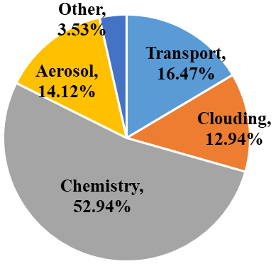
Figure 1 Typical fraction of time spent in the scientific processes in the source-oriented CMAQ model. This is based on a 36 km resolution domain (160 rows × 130 columns × 44 layers) and six source types and solved using the SMVGEAR solver.

The Euler backward iterative (EBI) approach (Hertel et al., 1993) is a faster method for solving the stiff ODE systems arising from a gas-phase photochemical mechanism. The basis of this method is the backward Euler method, as shown in Eq. (2):

$$\begin{array}{}\text{(2)}& C_{i,t}={\displaystyle \frac{C_{i,t-h}+h{P}_{i,t}}{\mathrm{1}+h{L}_{i,t}}},\end{array}$$

where C_i,t and $C_{i,t-h}$ are the concentrations of species i at time t and t−h, respectively; h is the integration time step; and P_i,t and L_i,t are the chemical production and loss terms, respectively, evaluated using the concentrations of the species at time t. Equation (2) represents a set of coupled non-linear equations, and a solution can be obtained by first evaluating the production and loss terms using the concentrations from the previous time step t−h to calculate an initial estimation of the species concentrations for the time step t based on Eq. (2). These concentrations are applied to update the P and L terms so that an updated estimation of the species concentrations for time step t is obtained. This procedure is repeated until the changes in C_i,t for a new iteration are less than a prescribed value.

For atmospheric photochemical reactions, there are several families of species whose concentrations are strongly coupled in reversible reactions. The general backward Euler method described above has a slow rate of convergence or even fails to converge. In the EBI solver, four family groups of strongly coupled species are excluded from the general Eq. (2): (1) NO, NO₂, O₃, and O(³P); (2) OH, HO₂, HONO, and HNO₄; (3) peroxyacetyl radical (CH₃C(O)OO^•, or C₂O₃) and peroxyacetyl nitrate (PAN); and (4) NO₃ and N₂O₅. For these species, analytical solutions of four sets of non-linear algebraic equations (Eqs. 9–12 in Hertel et al., 1993) are applied to determine their concentrations at time t instead of using the P and L terms with Eq. (2). The detailed mathematical procedures involved in obtaining these analytical solutions are listed in Appendices A.1–A.4 of Hertel et al. (1993).

The accuracy of the EBI solver has been evaluated against more accurate solvers (Hertel et al., 1993) and is the default choice in the CMAQ model for a number of built-in chemical mechanisms. However, it cannot be directly used to solve the source-oriented chemical mechanisms because the solution procedures of the aforementioned four strongly coupled groups calculate only the total concentrations of species, and source-tagged species are not included in the analytical solutions. Thus, for source-oriented mechanisms, groups of tagged reactive nitrogen species require additional solution steps. Direct replication of the procedures for total concentrations to treat the source-tagged species are infeasible, as this would dramatically increase the computational cost and the difficulty of source code implementation. An EBI solver capable of handling the chemical mechanisms with source-tagged species and their reactions while maintaining brevity and ease of implementation is highly desirable. Ideally, it should be able to predict the concentrations of source-tagged reactive nitrogen species based on their pre-determined total concentrations, which would greatly improve the computational efficiency and consequently enhance the applicability of the source-oriented air quality model.

The objective of this study is to develop a computationally efficient source-oriented gas-phase chemical mechanism for the simultaneous source apportionment of O₃ and other gaseous pollutants such as CO, primary VOCs, NO, NO₂, SO₂, and NH₃. The mechanism, when linked with a proper source-oriented aerosol mechanism, can be used to determine the source contributions to nitrate, sulfate, and ammonium ion. The method for improving the efficiency of the source-oriented mechanism through simplification of the reaction representation and modification of the EBI ODE solver for source-oriented nitrogen species is described in Sect. 2. Section 3 details the testing of the improved mechanism and the source-oriented EBI solver.

2 Method

2.1 Reduce the number of reactions and source-tagged species

In the original source-oriented model, a general reaction set that involves two source-tagged species as reactants for N_s source types can be written in the following form:

$$\begin{array}{}\text{(R9)}& \begin{array}{rl}& A_i+B_j\stackrel{k_{AB}}{⟶}{C}_i+D_j+E,\\ & i=\mathrm{1},\mathrm{2},\mathrm{\dots },N_{\mathrm{s}};j=\mathrm{1},\mathrm{2},\mathrm{\dots },N_{\mathrm{s}},\end{array}\end{array}$$

where A, B, C, and D are source-tagged model species and the subscripts denote the source origin index of these species. For simplicity, assume that C and D are the reaction products from A and B, respectively. E represents a general product whose source origin is not tracked in the model simulation. k_AB is the second-order reaction rate coefficient, which is the same for all the reactions in this reaction set. Reaction sets RS1 (Reactions R1–R4) and RS2 (Reactions R5–R8), as shown in the examples in Sect. 1, can both be expressed in this form. The loss rate of A_i is calculated using Eqs. (3a) and (3b):

$$\begin{array}{}\text{(3a)}& {\displaystyle }& {\displaystyle }\begin{array}{rl}{\displaystyle \frac{\mathrm{d}\left[A_i\right]}{\mathrm{d}t}}=& {\displaystyle }-k_{AB}\left[B_{\mathrm{1}}\right]\left[A_i\right]\mathrm{\dots }-k_{AB}\left[B_{N_{\mathrm{s}}}\right]\left[A_i\right],\\ {\displaystyle }& {\displaystyle }=-k_{A,\text{eff}B}\left[A_i\right],\end{array}\text{(3b)}& {\displaystyle }& {\displaystyle }{k}_{A,\text{eff}B}=k_{AB}\left[B_{\text{tot}}\right]=k_{\text{AB}}{\sum }_{j=\mathrm{1}}^{N_{\mathrm{s}}}\left[B_i\right],\end{array}$$

where k_A,effB is the pseudo-first-order reaction rate coefficient for [A_i] based on the total concentration of B, [B_tot], as defined in Eq. (3b). This method applies to reactions governed by bilinear rate laws, where the rate is proportional to the product of reactant concentrations (e.g., rate=k[A][B]). This form is prevalent in atmospheric chemistry, as most rate laws in apparent mechanisms are bimolecular. For termolecular reactions, their rate laws can be recursively converted into effective bimolecular representations using the same approach. A similar set of equations can be derived for the loss rate of individual tagged species B_i. Thus, the $N_{\mathrm{s}}^{\mathrm{2}}$ second-order reactions represented by Reaction (R9) can be equivalently described by the following 2N_s pseudo-first-order reactions:

$$\begin{array}{}\text{(R10)}& \begin{array}{rl}& A_i\stackrel{k_{A,\text{eff}B}}{⟶}{C}_i+E,i=\mathrm{1},\mathrm{2},\mathrm{\dots },N_{\mathrm{S}},\\ & B_i\stackrel{k_{B,\text{eff}A}}{⟶}{D}_i,i=\mathrm{1},\mathrm{2},\mathrm{\dots },N_{\mathrm{S}}.\end{array}\end{array}$$

For the non-typed product E, it can appear in either the A_i reactions or the B_i reactions, and it is easy to show that the formation rate of E based on Reaction (R10) is the same as these from Reaction (R9).

The dual-tagged N₂O₅ species and their reactions can be simplified as well. For ${{\mathrm{N}}_{\mathrm{2}}\mathrm{O}}_{\mathrm{5},ij}$, which represents N₂O₅ based on NO₂ from source i and NO₃ from source j, it can be equivalently written as $\mathrm{0.5}{\mathrm{N}}_{\mathrm{2}}{\mathrm{O}}_{\mathrm{5},\mathit{\text{i}}}+\mathrm{0.5}{\mathrm{N}}_{\mathrm{2}}{\mathrm{O}}_{\mathrm{5},\mathit{\text{j}}}$, as shown in Reaction (R11), in terms of preserving the source contributions to NO₂ and NO₃:

$$\begin{array}{}\text{(R11)}& \begin{array}{rl}& {\mathrm{NO}}_{\mathrm{2},i}+{\mathrm{NO}}_{\mathrm{3},j}\stackrel{k_{{\mathrm{NO}}_{\mathrm{2}}{\mathrm{NO}}_{\mathrm{3}}}}{⟶}\mathrm{0.5}{\mathrm{N}}_{\mathrm{2}}{\mathrm{O}}_{\mathrm{5},\mathit{\text{i}}}+\mathrm{0.5}{\mathrm{N}}_{\mathrm{2}}{\mathrm{O}}_{\mathrm{5},\mathit{\text{j}}},\\ & i=\mathrm{1},\mathrm{2},\mathrm{\dots },N_{\mathrm{s}};j=\mathrm{1},\mathrm{2},\mathrm{\dots },N_{\mathrm{s}}.\end{array}\end{array}$$

With this simplification, as well as the pseudo-first-order reaction technique described above, the reactions of N₂O₅ formation from N_s types of NO_x can be expanded into 2N_s reactions with N_s-tagged N₂O₅ species as shown in the general Reaction (R10), where A is NO₂, B is NO₃, and C and D are N₂O₅ species that have the same source tag as A and B, respectively. This dual-tagged reaction reduction method significantly decreases the number of species as well as the number of reactions for the source-oriented mechanism.

The total concentration of tagged species needed in Eq. (3b) for the pseudo-first-order reaction rate coefficient need not be tracked separately in the dual-tagged reaction reduction method. Instead, they are calculated on-the-fly and then used to calculate the pseudo-first-order rate coefficients for the reactions of the tagged species shown above. The function that calculates the reaction rates to be used in the stiff ODE solvers needs to be modified to recognize these special pseudo-first-order reactions. The CMAQ model is capable of dealing with these special pseudo-first-order reactions natively with its included mechanism preprocessor (CHEMMECH). An example input to the CHEMMECH on how the reactions are constructed for $\mathrm{NO}+{\mathrm{NO}}_{\mathrm{3}}\to \mathrm{2}{\mathrm{NO}}_{\mathrm{2}}$ for 10 source types is illustrated in Listing A1 of Appendix.

2.2 Source-oriented Euler backward iteration (EBI) scheme

2.2.1 Solution for family of source-tagged species in coupled reversible reactions

For source apportionment of ozone and secondary inorganic aerosols, the reactive nitrogen species NO, NO₂, HONO, HNO₄, PAN, NO₃, and N₂O₅ are source-tagged. For PAN, its source is determined by the source of NO₂, while the peroxyacetyl group is not source-tagged.

The standard solution procedure of the source-tagged species in the source-oriented EBI method includes two major steps: (1) evaluating total concentrations of these tagged species using equation sets (9–12) in Hertel et al. (1993) and (2) predicting the concentrations for each tagged species based on the total concentrations. In the following, the equations for step (1) are summarized first, followed by the equations for step (2). Equations are separately listed for each family.

The first set of equations, i.e., Eqs.(4a)–(4d), is used to solve the total concentrations of NO, NO₂, O₃, and O(³P). These equations are based on the corresponding ones in Hertel et al. (1993).

$$\begin{array}{}\text{(4a)}& {\displaystyle }& {\displaystyle }\begin{array}{rl}{\displaystyle }& {\displaystyle }[{\mathrm{NO}}_{\text{tot}}{]}_t=[{\mathrm{NO}}_{\text{tot}}{]}_{t-h}+h{P}_{\mathrm{1}}^{\prime }+h(r_{\mathrm{1},\mathrm{2}}+J_{\mathrm{1}})[{\mathrm{NO}}_{\mathrm{2},\mathrm{tot}}{]}_t\\ {\displaystyle }& {\displaystyle }-h{k}_{\mathrm{1},\mathrm{3}}\left[{\mathrm{O}}_{\mathrm{3}}{]}_t\right[{\mathrm{NO}}_{\text{tot}}{]}_t-h{r}_{\mathrm{2},\mathrm{1}}[{\mathrm{NO}}_{\text{tot}}{]}_t\\ {\displaystyle }& {\displaystyle }-h{L}_{\mathrm{1}}^{\prime }[{\mathrm{NO}}_{\text{tot}}{]}_t\end{array}\text{(4b)}& {\displaystyle }& {\displaystyle }\begin{array}{rl}{\displaystyle }& {\displaystyle }[{\mathrm{NO}}_{\mathrm{2},\mathrm{tot}}{]}_t=[{\mathrm{NO}}_{\mathrm{2},\mathrm{tot}}{]}_{t-h}+h{P}_{\mathrm{2}}^{\prime }+h{r}_{\mathrm{2},\mathrm{1}}[{\mathrm{NO}}_{\text{tot}}{]}_t\\ {\displaystyle }& {\displaystyle }+h{k}_{\mathrm{1},\mathrm{3}}\left[{\mathrm{O}}_{\mathrm{3}}{]}_t\right[{\mathrm{NO}}_{\text{tot}}{]}_t-h(r_{\mathrm{1},\mathrm{2}}+J_{\mathrm{1}})[{\mathrm{NO}}_{\mathrm{2},\mathrm{tot}}{]}_t\\ {\displaystyle }& {\displaystyle }-h{L}_{\mathrm{2}}^{\prime }[{\mathrm{NO}}_{\mathrm{2},\mathrm{tot}}{]}_t\end{array}\text{(4c)}& {\displaystyle }& {\displaystyle }\begin{array}{rl}{\displaystyle }& {\displaystyle }[{\mathrm{O}}_{\mathrm{3}}{]}_t=[{\mathrm{O}}_{\mathrm{3}}{]}_{t-h}+h{J}_{\mathrm{2}}[\mathrm{O}{(}^{\mathrm{3}}\mathrm{P}){]}_t-h{k}_{\mathrm{1},\mathrm{3}}[{\mathrm{NO}}_{\text{tot}}{]}_t[{\mathrm{O}}_{\mathrm{3}}{]}_t\\ {\displaystyle }& {\displaystyle }-h{L}_{\mathrm{3}}^{\prime }[{\mathrm{O}}_{\mathrm{3}}{]}_t\end{array}\text{(4d)}& {\displaystyle }& {\displaystyle }\begin{array}{rl}{\displaystyle }& {\displaystyle }[\mathrm{O}{(}^{\mathrm{3}}\mathrm{P}){]}_t=[\mathrm{O}{(}^{\mathrm{3}}\mathrm{P}){]}_{t-h}+h{P}_{\mathrm{12}}^{\prime }+h{J}_{\mathrm{1}}[{\mathrm{NO}}_{\mathrm{2},\mathrm{tot}}{]}_t\\ {\displaystyle }& {\displaystyle }-h{J}_{\mathrm{2}}[\mathrm{O}{(}^{\mathrm{3}}\mathrm{P}){]}_t-h{L}_{\mathrm{12}}^{\prime }[\mathrm{O}{(}^{\mathrm{3}}\mathrm{P}){]}_t\end{array}\end{array}$$

In the above equations, species with a subscript “tot” represent the total concentration of a set of tagged species, which is calculated by adding the concentrations of the individual tagged species; h is the size of the current time step; r_1,2 is the production rate coefficient of NO from NO₂, excluding photo-dissociation; J₁ is the photolysis rate of NO₂ to form NO; k_1,3 is the second-order rate coefficient for the NO+O₃ reaction to form NO₂; and r_2,1 is the pseudo-first-order rate constant for the production of NO₂ from NO from all other pathways, excluding the NO+O₃ reaction. J₂ is the first-order reaction rate constant for O(³P)+O₂ to form O₃. The terms $P_{\mathrm{1}}^{\prime }$, $P_{\mathrm{2}}^{\prime }$, and $P_{\mathrm{12}}^{\prime }$ account for all the remaining production for the total concentrations of NO, NO₂, and O(³P) in the mechanism, and the terms $L_{\mathrm{1}}^{\prime }$, $L_{\mathrm{2}}^{\prime }$, $L_{\mathrm{3}}^{\prime }$, and $L_{\mathrm{12}}^{\prime }$ are the losses of the total concentrations of NO, NO₂, O₃, and O(³P), respectively. Analytical solutions for the total concentrations based on Eqs. (4a)–(4d) were derived and described in detail in Appendix A of Hertel et al. (1993) and are not repeated here.

Once the total concentrations of NO, NO₂, O₃, and O(³P) are solved, concentrations of the source-tagged NO and NO₂ are solved from the following two equations:

$$\begin{array}{}\text{(5a)}& {\displaystyle }& {\displaystyle }\begin{array}{rl}{\displaystyle }& {\displaystyle }[{\mathrm{NO}}_i{]}_t=[{\mathrm{NO}}_i{]}_{t-h}+h{P}_{\mathrm{1},i}^{\prime }+h(r_{\mathrm{1},\mathrm{2}}+J_{\mathrm{1}})[{\mathrm{NO}}_{\mathrm{2},i}{]}_t\\ {\displaystyle }& {\displaystyle }-h{k}_{\mathrm{1},\mathrm{3}}\left[{\mathrm{O}}_{\mathrm{3}}{]}_t\right[{\mathrm{NO}}_i{]}_t-h{r}_{\mathrm{2},\mathrm{1}}[{\mathrm{NO}}_i{]}_t-h{L}_{\mathrm{1}}^{\prime }[{\mathrm{NO}}_i{]}_t,\end{array}\text{(5b)}& {\displaystyle }& {\displaystyle }\begin{array}{rl}{\displaystyle }& {\displaystyle }[{\mathrm{NO}}_{\mathrm{2},i}{]}_t=[{\mathrm{NO}}_{\mathrm{2},i}{]}_{t-h}+h{P}_{\mathrm{2},i}^{\prime }+h{r}_{\mathrm{2},\mathrm{1}}[{\mathrm{NO}}_i{]}_t\\ {\displaystyle }& {\displaystyle }+h{k}_{\mathrm{1},\mathrm{3}}\left[{\mathrm{O}}_{\mathrm{3}}{]}_t\right[{\mathrm{NO}}_i{]}_t-h(r_{\mathrm{1},\mathrm{2}}+J_{\mathrm{1}})[{\mathrm{NO}}_{\mathrm{2},i}{]}_t\\ {\displaystyle }& {\displaystyle }-h{L}_{\mathrm{2}}^{\prime }[{\mathrm{NO}}_{\mathrm{2},i}{]}_t,\end{array}\end{array}$$

where i is the source index for the tagged species. For each i, the two unknowns [NO_i]_t and [NO_2,i]_t are solved analytically using the following equations:

$$\begin{array}{}\text{(6a)}& {\displaystyle }[{\mathrm{NO}}_i{]}_t={\displaystyle \frac{\mathrm{1}}{\text{det}\left(\mathbf{A}\right)}}(A_{\mathrm{22}}{b}_{\mathrm{1}}-A_{\mathrm{12}}{b}_{\mathrm{2}}),\text{(6b)}& {\displaystyle }[{\mathrm{NO}}_{\mathrm{2},i}{]}_t={\displaystyle \frac{\mathrm{1}}{\text{det}\left(\mathbf{A}\right)}}(-A_{\mathrm{21}}{b}_{\mathrm{1}}+A_{\mathrm{11}}{b}_{\mathrm{2}}),\text{(6c)}& {\displaystyle }\mathbf{A}=\left[\begin{array}{cc}\mathrm{1}+h{k}_{\mathrm{1},\mathrm{3}}[{\mathrm{O}}_{\mathrm{3}}{]}_t+h{r}_{\mathrm{1},\mathrm{2}}+h{L}_{\mathrm{1}}^{\prime }& -h(r_{\mathrm{2},\mathrm{1}}+J_{\mathrm{1}})\\ -h(r_{\mathrm{2},\mathrm{1}}+k_{\mathrm{1},\mathrm{3}}[{\mathrm{O}}_{\mathrm{3}}{]}_t)& \mathrm{1}+h{r}_{\mathrm{1},\mathrm{2}}+h{J}_{\mathrm{1}}+h{L}_{\mathrm{2}}^{\prime }\end{array}\right],\text{(6d)}& {\displaystyle }\mathbf{b}=\left[\begin{array}{c}[{\mathrm{NO}}_i{]}_{t-h}+h{P}_{\mathrm{1},i}^{\prime }\\ [{\mathrm{NO}}_{\mathrm{2},i}{]}_{t-h}+h{P}_{\mathrm{2},i}^{\prime }\end{array}\right].\end{array}$$

In Eqs. (6a) and (6b), det(A) is the determinant of the 2×2 matrix A, as defined in Eq. (6c).

The second set of equations is for the total concentrations of OH, HO₂, HONO, and HNO₄, as shown in Eqs. (7a)–(7d).

$$\begin{array}{}\text{(7a)}& {\displaystyle }& {\displaystyle }\begin{array}{rl}{\displaystyle }& {\displaystyle }[\mathrm{OH}{]}_t=[\mathrm{OH}{]}_{t-h}+h{P}_{\mathrm{4}}^{\prime }+h{r}_{\mathrm{4},\mathrm{5}}[{\mathrm{HO}}_{\mathrm{2}}{]}_t\\ {\displaystyle }& {\displaystyle }+h{r}_{\mathrm{4},\mathrm{19}}[{\mathrm{HONO}}_{\text{tot}}{]}_t-h{L}_{\mathrm{4}}[\mathrm{OH}{]}_t\end{array}\text{(7b)}& {\displaystyle }& {\displaystyle }\begin{array}{rl}{\displaystyle }& {\displaystyle }[{\mathrm{HO}}_{\mathrm{2}}{]}_t=[{\mathrm{HO}}_{\mathrm{2}}{]}_{t-h}+h{P}_{\mathrm{5}}^{\prime }+h{r}_{\mathrm{5},\mathrm{4}}[\mathrm{OH}{]}_t\\ {\displaystyle }& {\displaystyle }+h{r}_{\mathrm{5},\mathrm{21}}[{\mathrm{HNO}}_{\mathrm{4},\mathrm{tot}}{]}_t-\mathrm{2}h{k}_{\mathrm{5},\mathrm{5}}[{\mathrm{HO}}_{\mathrm{2}}{]}_t^{\mathrm{2}}-h{L}_{\mathrm{5}}^{\prime }[{\mathrm{HO}}_{\mathrm{2}}{]}_t\end{array}\text{(7c)}& {\displaystyle }& {\displaystyle }\begin{array}{rl}{\displaystyle }& {\displaystyle }[{\mathrm{HONO}}_{\text{tot}}{]}_t=[{\mathrm{HONO}}_{\text{tot}}{]}_{t-h}+h{r}_{\mathrm{19},\mathrm{4}}[\mathrm{OH}{]}_t\\ {\displaystyle }& {\displaystyle }-h{L}_{\mathrm{19}}[{\mathrm{HONO}}_{\text{tot}}{]}_t\end{array}\text{(7d)}& {\displaystyle }& {\displaystyle }\begin{array}{rl}{\displaystyle }& {\displaystyle }[{\mathrm{HNO}}_{\mathrm{4},\mathrm{tot}}{]}_t=[{\mathrm{HNO}}_{\mathrm{4},\mathrm{tot}}{]}_{t-h}+h{r}_{\mathrm{21},\mathrm{5}}[{\mathrm{HO}}_{\mathrm{2}}{]}_t\\ {\displaystyle }& {\displaystyle }-h{L}_{\mathrm{21}}[{\mathrm{HNO}}_{\mathrm{4},\mathrm{tot}}{]}_t\end{array}\end{array}$$

The notations and symbols used in the above equations are similar to those used in Eqs. (4a)–(4d). r_4,5 and r_4,19 are pseudo-first-order production rate coefficients of OH from HO₂ and HONO, respectively. r_5,4 and r_5,21 are pseudo-first-order production rate coefficients of HO₂ from OH and HNO₄, respectively. k_5,5 is the HO₂+HO₂ self-reaction rate coefficient. r_19,4 and r_21,5 are pseudo-first-order rate coefficients for the production of HONO and HNO₄ from OH+NO and HO₂+NO₂, respectively. The terms $P_{\mathrm{4}}^{\prime }$ and $P_{\mathrm{5}}^{\prime }$ account for all the remaining production of OH and HO₂, and the terms L₄, $L_{\mathrm{5}}^{\prime }$, L₁₉, and L₂₁ account for all the other losses of OH, HO₂, HONO, and HNO₄, respectively. Analytical solutions for Eqs. (7a)–(7d) were also derived and described in detail in Appendix A of Hertel et al. (1993). As the OH and HO₂ concentrations are determined, concentrations of individual HONO and HNO₄ from different sources are solved using Eqs. (8a) and (8b), respectively.

$$\begin{array}{}\text{(8a)}& {\displaystyle }& {\displaystyle }[{\mathrm{HONO}}_i{]}_t={\displaystyle \frac{[{\mathrm{HONO}}_i{]}_{t-h}+h{r}_{\mathrm{19},\mathrm{4}}^i[\mathrm{OH}{]}_t}{\mathrm{1}+h{L}_{\mathrm{19}}}}\text{(8b)}& {\displaystyle }& {\displaystyle }[{\mathrm{HNO}}_{\mathrm{4},i}{]}_t={\displaystyle \frac{[{\mathrm{HNO}}_{\mathrm{4},i}{]}_{t-h}+h{r}_{\mathrm{21},\mathrm{5}}^i[{\mathrm{HO}}_{\mathrm{2}}{]}_t}{\mathrm{1}+h{L}_{\mathrm{21}}}}\end{array}$$

Here, $r_{\mathrm{19},\mathrm{4}}^i$ and $r_{\mathrm{21},\mathrm{5}}^i$ are pseudo-first-order production rate coefficients of HONO and HNO₄ from source i due to NO and NO₂ from the same source with OH and HO₂, respectively. Concentrations of NO_i and NO_2,i for the current time step have already been determined using Eq. (6a) and (6b), and these concentrations will be applied to calculate $r_{\mathrm{19},\mathrm{4}}^i$ and $r_{\mathrm{21},\mathrm{5}}^i$ used in the above two equations.

The third set of equations is for C₂O₃ and PAN:

$$\begin{array}{}\text{(9a)}& {\displaystyle }& {\displaystyle }\begin{array}{rl}{\displaystyle }& {\displaystyle }[{\mathrm{C}}_{\mathrm{2}}{\mathrm{O}}_{\mathrm{3}}{]}_t=[{\mathrm{C}}_{\mathrm{2}}{\mathrm{O}}_{\mathrm{3}}{]}_{t-h}+h{P}_{\mathrm{8}}^{\prime }+h{r}_{\mathrm{8},\mathrm{9}}[{\mathrm{PAN}}_{\text{tot}}{]}_t\\ {\displaystyle }& {\displaystyle }-\mathrm{2}h{k}_{\mathrm{8},\mathrm{8}}[{\mathrm{C}}_{\mathrm{2}}{\mathrm{O}}_{\mathrm{3}}{]}_t^{\mathrm{2}}-h{L}_{\mathrm{8}}^{\prime }[{\mathrm{C}}_{\mathrm{2}}{\mathrm{O}}_{\mathrm{3}}{]}_t,\end{array}\text{(9b)}& {\displaystyle }& {\displaystyle }\begin{array}{rl}{\displaystyle }& {\displaystyle }[{\mathrm{PAN}}_{\text{tot}}{]}_t=[{\mathrm{PAN}}_{\text{tot}}{]}_{t-h}+h{r}_{\mathrm{9},\mathrm{8}}[{\mathrm{C}}_{\mathrm{2}}{\mathrm{O}}_{\mathrm{3}}{]}_t\\ {\displaystyle }& {\displaystyle }-h{L}_{\mathrm{9}}[{\mathrm{PAN}}_{\text{tot}}{]}_t.\end{array}\end{array}$$

In the equations, it is assumed that, in the source-oriented mechanism, PAN is a source-tagged species and its source is based on the source of NO₂, whereas C₂O₃ is not source-tagged. This is sufficient for the source apportionment of ozone, as described in Sect. 2.1. A quadratic equation for C₂O₃ can be obtained (see Appendix A of Hertel et al., 1993). In r_9,8, the total NO₂ concentration at the current time step t has already been determined by solving Eqs. (4a)–(4d). Once the concentrations of C₂O₃ at time step t are solved, the concentrations of each of the tagged PAN species can be used as follows:

$$\begin{array}{}\text{(9c)}& [{\mathrm{PAN}}_i{]}_t={\displaystyle \frac{[{\mathrm{PAN}}_i{]}_{t-h}+h{r}_{\mathrm{9},\mathrm{8}}^i[{\mathrm{C}}_{\mathrm{2}}{\mathrm{O}}_{\mathrm{3}}{]}_t}{\mathrm{1}+h{L}_{\mathrm{21}}}},\end{array}$$

where $r_{\mathrm{9},\mathrm{8}}^i$ includes the concentration of NO_2,i (NO₂ attributed to source i) at the current time step t.

The last set of equations treated in the source-oriented EBI solver is for NO₃ and N₂O₅, as shown in Eq. (10).

$$\begin{array}{}\text{(10a)}& {\displaystyle }& {\displaystyle }\begin{array}{rl}{\displaystyle }& {\displaystyle }[{\mathrm{NO}}_{\mathrm{3},\mathrm{tot}}{]}_t=[{\mathrm{NO}}_{\mathrm{3},\text{tot}}{]}_{t-h}+h{P}_{\mathrm{15}}^{\prime }\\ {\displaystyle }& {\displaystyle }+h{r}_{\mathrm{15},\mathrm{16}}[{\mathrm{N}}_{\mathrm{2}}{\mathrm{O}}_{\mathrm{5},\mathrm{tot}}{]}_t-h{L}_{\mathrm{15}}[{\mathrm{NO}}_{\mathrm{3},\mathrm{tot}}{]}_t\end{array}\text{(10b)}& {\displaystyle }& {\displaystyle }\begin{array}{rl}{\displaystyle }& {\displaystyle }[{\mathrm{N}}_{\mathrm{2}}{\mathrm{O}}_{\mathrm{5},\mathrm{tot}}{]}_t=[{\mathrm{N}}_{\mathrm{2}}{\mathrm{O}}_{\mathrm{5},\mathrm{tot}}{]}_{t-h}+h{r}_{\mathrm{16},\mathrm{15}}[{\mathrm{NO}}_{\mathrm{3},\mathrm{tot}}{]}_t\\ {\displaystyle }& {\displaystyle }-h{L}_{\mathrm{16}}[{\mathrm{N}}_{\mathrm{2}}{\mathrm{O}}_{\mathrm{5},\mathrm{tot}}{]}_t\end{array}\end{array}$$

The two equations are linear equations and can be solved easily for NO_3,tot and N₂O_5,tot. Both NO_3,i and ${{\mathrm{N}}_{\mathrm{2}}\mathrm{O}}_{\mathrm{5},i}$ (as discussed in Sect. 2.1, sources of N₂O₅ can be tracked with a single type instead of a double type) can be solved analytically based on the two equations as well, as shown in Eqs. (10c) and (10d).

$$\begin{array}{}\text{(10c)}& {\displaystyle }& {\displaystyle }\begin{array}{r}{\displaystyle }[{\mathrm{NO}}_{\mathrm{3},i}{]}_t={\displaystyle \frac{\begin{array}{l}(\mathrm{1}+h{L}_{\mathrm{16}})\left([{\mathrm{NO}}_{\mathrm{3},i}{]}_{t-h}+h{P}_{\mathrm{15}}^{i{,}^{\prime }}\right)\\ +h{r}_{\mathrm{15},\mathrm{16}}[{\mathrm{N}}_{\mathrm{2}}{\mathrm{O}}_{\mathrm{5},\mathrm{tot}}{]}_{t-h}\end{array}}{(\mathrm{1}+h{L}_{\mathrm{15}})(\mathrm{1}+h{L}_{\mathrm{16}})-h^{\mathrm{2}}{r}_{\mathrm{15},\mathrm{16}}{r}_{\mathrm{16},\mathrm{15}}}}\end{array}\text{(10d)}& {\displaystyle }& {\displaystyle }\begin{array}{r}{\displaystyle }[{{\mathrm{N}}_{\mathrm{2}}\mathrm{O}}_{\mathrm{5},i}{]}_t={\displaystyle \frac{\begin{array}{l}(\mathrm{1}+h{L}_{\mathrm{15}})[{\mathrm{N}}_{\mathrm{2}}{\mathrm{O}}_{\mathrm{5},\mathrm{tot}}{]}_{t-h}\\ +h{r}_{\mathrm{16},\mathrm{15}}\left([{\mathrm{NO}}_{\mathrm{3},i}{]}_{t-h}+h{P}_{\mathrm{15}}^{i{,}^{\prime }}\right)\end{array}}{(\mathrm{1}+h{L}_{\mathrm{15}})(\mathrm{1}+h{L}_{\mathrm{16}})-h^{\mathrm{2}}{r}_{\mathrm{15},\mathrm{16}}{r}_{\mathrm{16},\mathrm{15}}}}\end{array}\end{array}$$

Note that r_16,15 includes the total concentration of NO₂ and thus is the same as that used in Eq. (10b). However, the production of NO₃ from other reactions does have to be source-specific; thus, the P15's used in Eqs. (10c) and (10a) are different.

To avoid round-off errors introduced in the calculation for the source-tagged species involved in these four groups so that the sum of the source-tagged species always exactly matches the total concentrations, their concentrations are readjusted by the pre-determined total concentrations of photochemical species by solving the algebraic equations for the special groups in the original EBI scheme.

2.2.2 Successive under-relaxation

During the testing of the above algorithm, non-converging oscillations were sometimes observed, mostly due to the low concentration of source-tagged species. The iterative process used in the EBI solver can be modified to include a relaxation factor α so that the concentration array at the end of each iteration is updated by a weighted average of the results from the previous iteration and the present estimated values in the current iteration, as shown in Eq. (11).

$$\begin{array}{}\text{(11)}& C_{i,\text{iter}}^{\text{update}}=(\mathrm{1}-\mathit{\alpha })C_{i,\text{iter}-\mathrm{1}}+\mathit{\alpha }{C}_{i,\text{iter}}\end{array}$$

The selection of α influences only the number of iterations required for convergence, not the final converged solutions. Generally, larger α values lead to faster convergence but have a higher chance of falling into oscillation. Based on the testing, α=0.8 appears to be a conservative choice that always leads to convergence. A dynamic under-relaxation scheme using a set of varying α values between 0.79 and 1.0, based on the number of iterations in the EBI scheme, is shown to lead to faster convergence. This is further discussed in the Results section.

Table 1 Computation time needed for a 1 d simulation using two different versions of the source-oriented chemical mechanism and two versions of the ODE solvers. Both versions are capable of tracking 10 different source types in a single simulation.

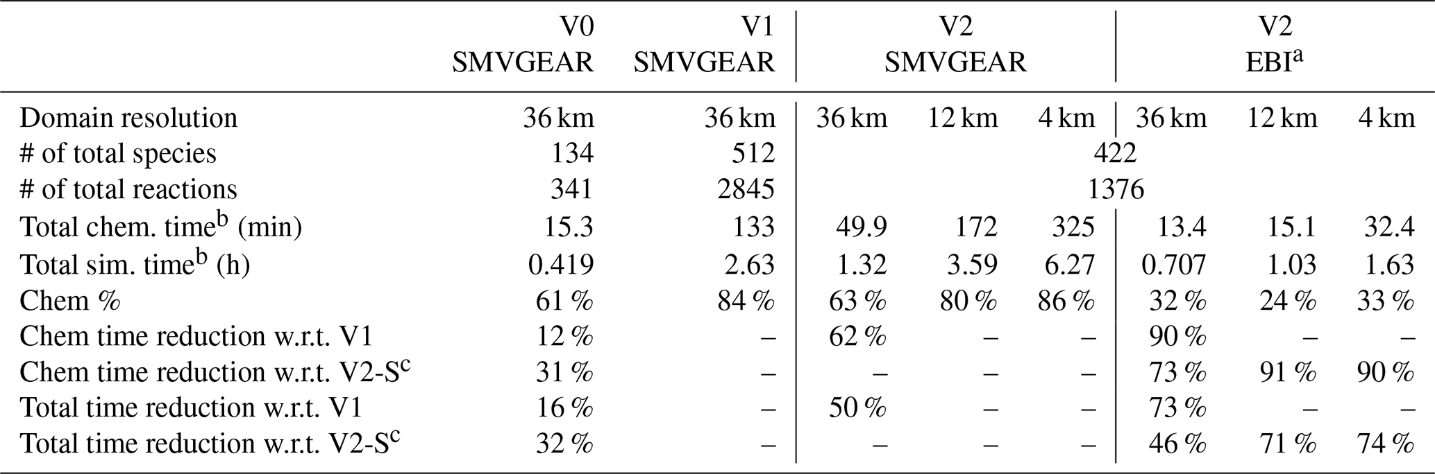
^a Simulation time based on dynamic under-relaxation coefficient. ^b Wall-clock time. ^c V2-S: V2 reaction mechanism with SMVGEAR solver.

2.3 Test mechanism and model setup

To evaluate how much improvement in computational efficiency can be achieved by using the simplified reaction representation and source-oriented EBI solver, a series of source-oriented mechanisms for simultaneous attribution of ozone and secondary inorganic aerosol was constructed based on the SAPRC-07 photochemical mechanism and implemented in CMAQv5.2. The SAPRC-07 mechanism is chosen instead of the more recent versions of SAPRC because it is faster with fewer species and reactions and thus is more suitable for simulations requiring rapid response, such as operational air quality forecasting and for source apportionment of ozone and secondary inorganic aerosols. The source-oriented mechanism based on this will be applied in a future air quality forecasting model that also forecasts source-tagged species concentrations and source-region contributions to air pollution. As the primary goal of this paper is to evaluate the efficiency of the gas-phase algorithm, aerosol results, despite being enabled in the simulations along with cloud processes, are not included in the analyses described below.

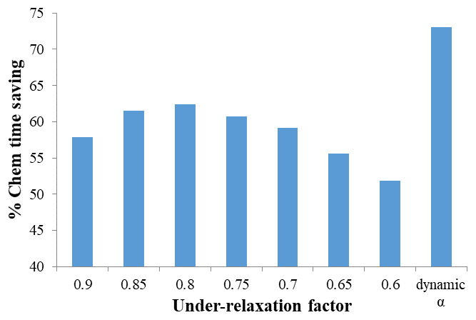
Figure 2 Percentage chemistry time saving with respect to the SMVGEAR solver for the identical source-oriented chemical mechanism for the 36 km domain. See text and Table 2 for the details of the dynamic under-relaxation scheme.

The tested SAPRC-07 mechanism used in this study contains a total of 134 species and 341 reactions. Among these species, 15 species are reactive nitrogen species. For each of these species, tagged species are used to track their source origins. Reactions involving these species are expanded in the source-oriented mechanism. In addition, CO, SO₂, and sulfuric acid (SULF) are also expanded in the source-oriented mechanism. To evaluate source contributions to ozone, 14 primary VOC species are also treated as source-oriented species in addition to source-tagged non-reactive O₃ species to track contributions from different sources of NO_x and VOCs to O₃ formation. As HCHO is an important oxidation product from several parent VOCs, sources of secondary HCHO from the first-generation oxidation of parent VOCs are also tracked. Details regarding the source apportionment of O₃ have been given by Wang et al. (Wang et al., 2019a, b) and are not repeated here. While the dual-tagged reaction reduction method and EBI solver for source apportionment can be employed separately, their integration could lead to enhanced performance and more significant benefits. Two versions of the source-oriented SAPRC-07 mechanisms are prepared. The first version (V1) uses dual-tagged N₂O₅ and fully expanded reactions without the pseudo-first-order reactions described in Sect. 2. The second version (V2) is based on single-tagged N₂O₅ and a dual-tagged reaction reduction treatment applied to the fully expanded V1 mechanism, as described in Sect. 2.1. Both mechanisms are constructed to track emissions from 10 source types. The number of reactions and species in each mechanism is listed in Table 1, while the accuracy of this method is presented in Fig. A1, which shows the EBI solver's predictions scattered on the 1:1 line when compared to the SMVGEAR solver's results for tagged species concentrations and the total.

Table 2 Dynamic section of the under-relaxation factor (α) based on the iteration count.

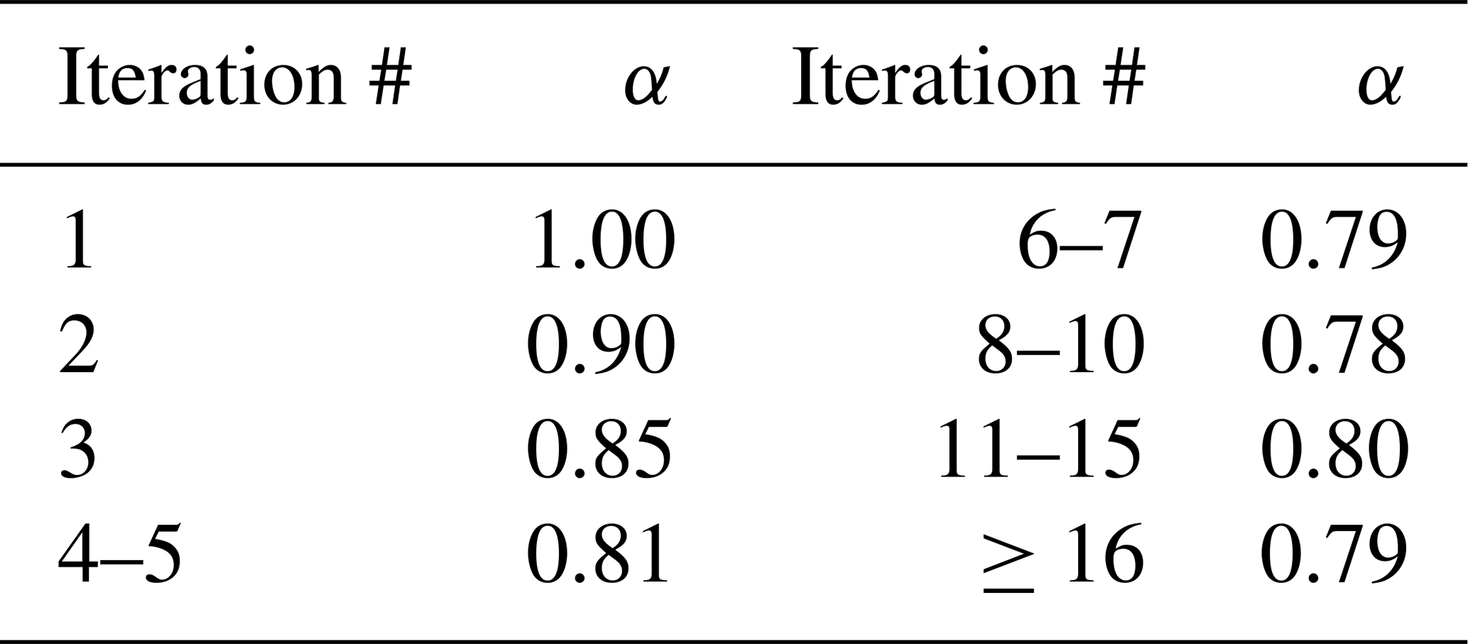
Table 3 Max and mean values of the normalized error* for selected species in the 36 km domain.

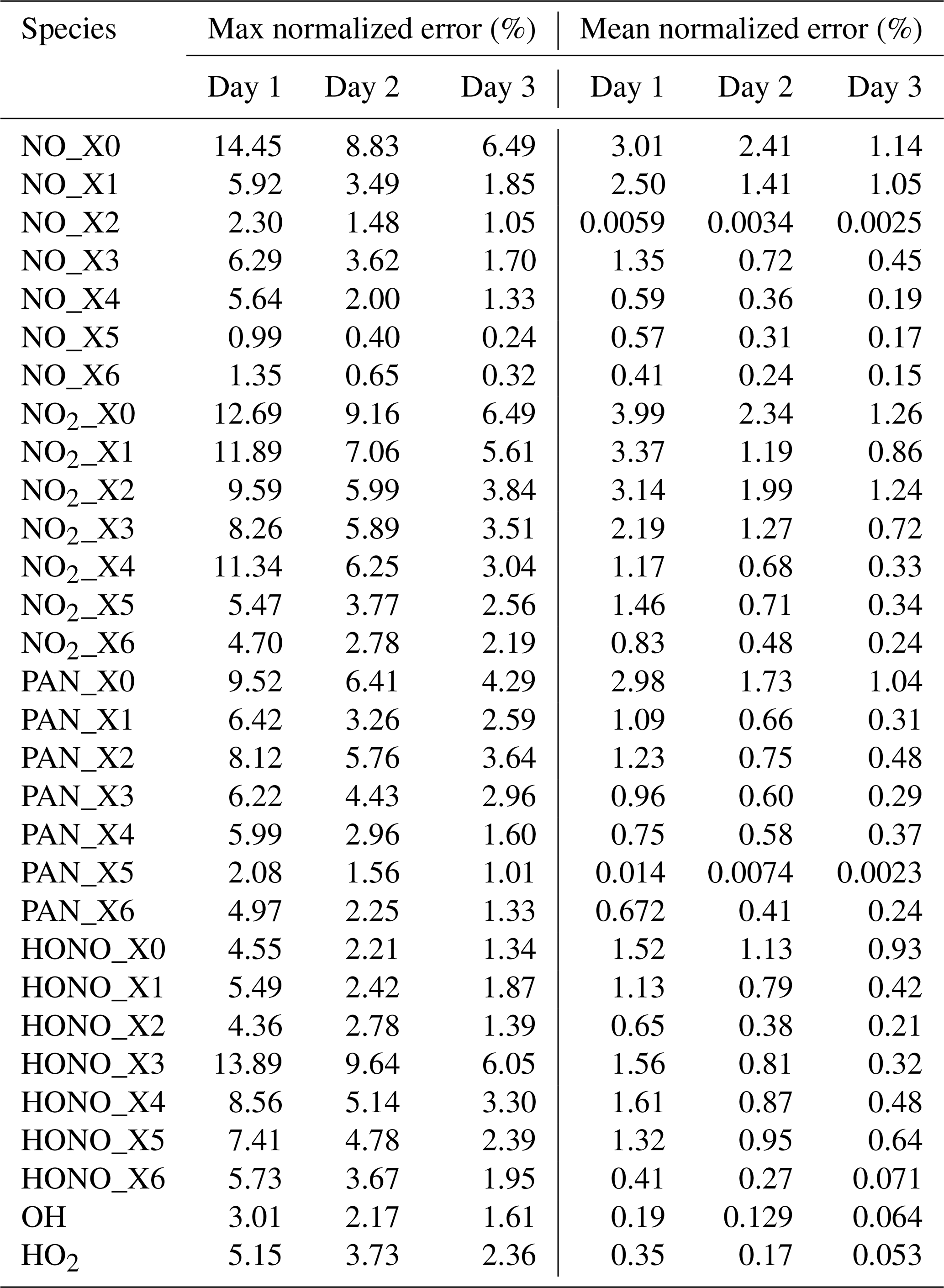
* Normalized error is calculated as $|C_{\text{V2-EBI}}-C_{\text{V2-SMVGEAR}}|/C_{\text{V2\_SMVGEAR}}$. This is calculated for hourly concentrations for all the grid cells in the entire day. The mean normalized error is calculated by averaging the normalized error for all the grid cells.

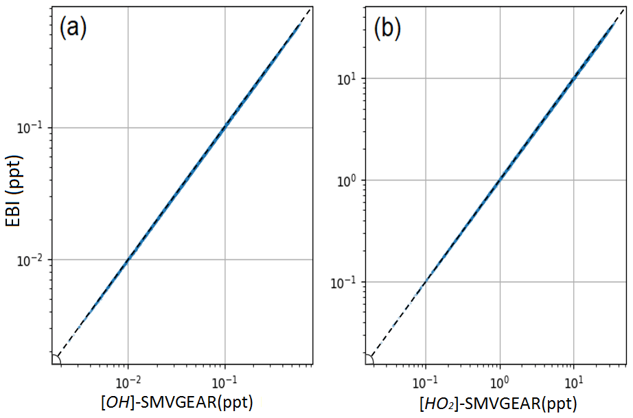
Figure 3 Comparison of predicted OH (a) and HO₂ (b) radicals in the surface layer of the 36 km resolution domain using the source-oriented EBI (new) and the SMVGEAR (baseline) solvers. Concentrations at hour 6 (local time 14:00–15:00) are shown.

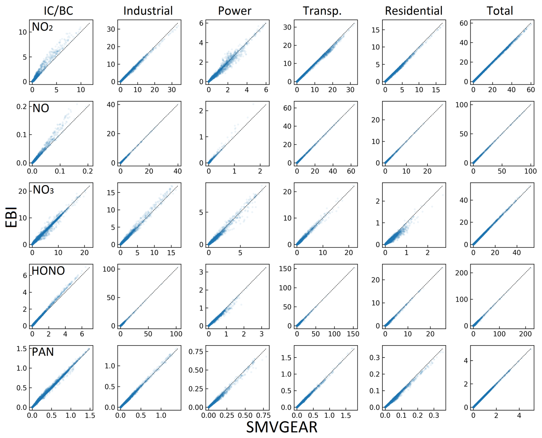
Figure 4 Predicted hourly averaged NO₂, NO, NO₃, HONO, and PAN concentrations for different source types in the last hour of the day-1 simulation using the source-oriented EBI (new) and SMVGEAR (baseline) solvers. Concentrations of all grid cells in the surface layer are included in the plot. Concentrations are in units of ppb for NO, NO₂, and PAN and in units of ppt for NO₃ and HONO.

The testing is performed for a 3 d (1–3 July 2020) simulation using three-level nested domains with 36, 12, and 4 km resolutions that cover eastern Asia, central and eastern China, and the Henan province in central China, respectively. The meteorology inputs were based on the Weather Research and Forecasting (WRF) model v4.1.4. The anthropogenic emissions are based on the Multi-scale Emission Inventory for China (MEIC, for the 36 and 12 km domains, available from http://www.meicmodel.org/, last access: 10 June 2025) and a local emission inventory (for the 4 km domain) (Lu et al., 2023). Emissions are grouped into six source categories, including five anthropogenic source sectors (power, industrial, residential, transportation, and agriculture) and one biogenic sector, whose emission is based on MEGAN (Model for Emissions of Gases and Aerosol from Nature) v2.1(Guenther et al., 2006). The initial concentrations of the species are based on a 7 d non-source-oriented simulation. The boundary conditions for the 36 km domain are based on the clean continental vertical profiles included in the CMAQ model. The boundary conditions of the 12 and 4 km domains are based on results from the parent 36 and 12 km domains, respectively.

Three sets of simulations using the source-oriented mechanisms were conducted: (1) V1, solved using the SMVGEAR solver (V1-GEAR), (2) V2, solved with SMVGEAR (V2-GEAR), and (3) V2, solved with the source-oriented EBI (V2-EBI). For SMVGEAR, a relative tolerance (RTOL) of $\mathrm{1}\times {\mathrm{10}}^{-\mathrm{3}}$ and an absolute tolerance (ATOL) of $\mathrm{1}\times {\mathrm{10}}^{-\mathrm{9}}$ were used. For the EBI solver, only a relative tolerance RTOL was used in the convergence check. For most of the species, a relative tolerance of $\mathrm{1}\times {\mathrm{10}}^{-\mathrm{3}}$ was used. Exceptions include pseudo-steady-state species like O₃P and O₁D, for which a tolerance of 1.0 was applied, indicating that a convergence check is not applicable. Integrated reaction rate (IRR) analysis was used in all three simulations, as it is needed for the ozone source apportionment algorithm (Wang et al., 2019b). In addition to the source-oriented model simulations, two base case simulations (V0) were conducted using the unmodified SAPRC-07 solved with the SMVGEAR (V0-SMVGEAR) and EBI (V0-EBI) solvers, respectively.

All the simulations were conducted on a Dell Precision-Tower 7810 working station (2XE-2660-v4, 28/56 cores/threads, and 256G of DDR4 RAM), and the run was in parallel in a configuration of 8×6 domain decomposition.

3 Results

3.1 Timing results

For the first day of simulation, the wall-clock time for the gas-phase mechanism as well as the total run time were recorded using the time function (MPI_WTIME) in the Message Passing Interface. An MPI_BARRIER call was issued before each MPI_TIME call to make sure that the measured wall-clock time represents the actual time for a chemistry time step in a static domain decomposition setting with imbalanced loads.

The wall-clock time for the 1 d simulation using the source-oriented EBI solver was compared with the SMVGEAR solver and presented in Table 1. The fully expanded source-oriented mechanism with SMVGEAR (V1-SMVGEAR) is the slowest, and only the 36 km resolution simulation was conducted. The simplified reaction representation alone (V2-SMVGEAR, see Sect. 2.1) led to a reduction in chemistry time by ∼62 % when compared with V1-SMVGEAR (133–49.9 min) and a reduction in the total computation time by ∼50 % (2.63–1.32 h). Using the source-oriented EBI on V2 (V2-EBI) further reduced the total chemistry time to ∼13.4 min. Compared to V1-SMVGEAR, V2-EBI reduced the chemistry time by ∼90 % and the total time by ∼75 % for a 1 d simulation in the 36 km domain.

The EBI solver represents a significant reduction in both chemistry time and total computation time compared to the SMVGEAR solver. When V2-SMVGEAR and V2-EBI are compared, the total chemistry time saving of the EBI scheme increases with grid resolution, from 70 % for 36 km to 90 % for 4 km. As a result, the total simulation time saving increases from 46 % for a coarse grid to 74 % for a fine grid. The increase in time saving of the EBI solver with grid resolution can be attributed to the smaller time step size, which is determined from the flow Courant stability criterion. For a fixed simulation duration (1 d in this study), the required total number of chemistry steps increases dramatically with grid resolution, which results in a significant reduction in total chemistry time with the faster EBI scheme for a finer grid. Therefore, for time-consuming applications such as long-term source apportionment simulation of nested domains, the time efficiency can be improved by a factor of 3 or more.

The V2-EBI results shown in Table 1 are based on the dynamic under-relaxation using an iteration-count-dependent under-relaxation factor (α) shown in Table 2. In this scheme, α is initially set to 1.0 and gradually decreases to smaller values. If the solution does not converge in 15 iterations, a constant α of 0.79 is used. Using this dynamic α scheme is demonstrated to be more efficient than using a constant α, as shown in Fig. 2. The optimal value for fixed α is 0.8, at which the total chemistry time could be reduced by ∼62 %, for the 36 km domain simulations, which is approximately 10 % less than the dynamic α scheme.

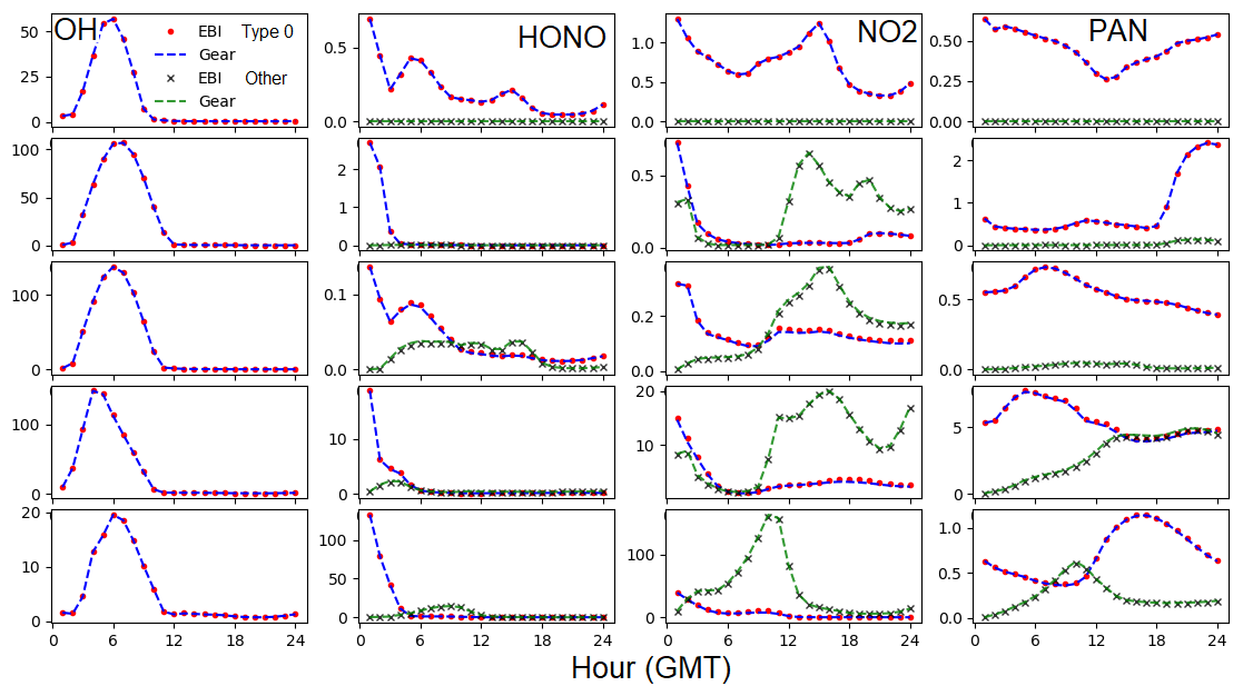
Figure 5 Time series of OH, HONO, NO₂, and PAN at grid cells that represent different emission conditions (no emissions, low emission, medium emission, high emission, and intense emission) for the 1 d simulation. Units are ppq (parts per quadrillion) for OH, ppt for HONO, and 0.1 ppb for NO₂ and PAN. Type 0 is the concentration for the IC/BC source type, and “Other” represents the sum of the concentrations of all other tagged species.

The values of α in Table 2 have been fine-tuned through a series of numerical experiments to optimize the convergence rate for the source-oriented chemical mechanisms. The dynamic α strategy demonstrates superior performance due to its adaptive nature. Larger α values in the early iterations aggressively propel a rapid movement of the solution vector towards the region of the true solution. Subsequently, in later iterations, a more conservative approach with smaller α values is adopted to gradually refine the solution and effectively damp out residual errors and potential overshoots by assigning more weight to the solution of the previous iteration. For the majority of test cases, convergence is achieved within 10 iterations. However, in instances where convergence is slower, a slightly larger adjustment step (an increase in α between iterations 11 and 15) can be beneficial for a faster approach to the true solution. The ultimate value of α=0.79 is aimed at effectively damping oscillations in the final convergence stages.

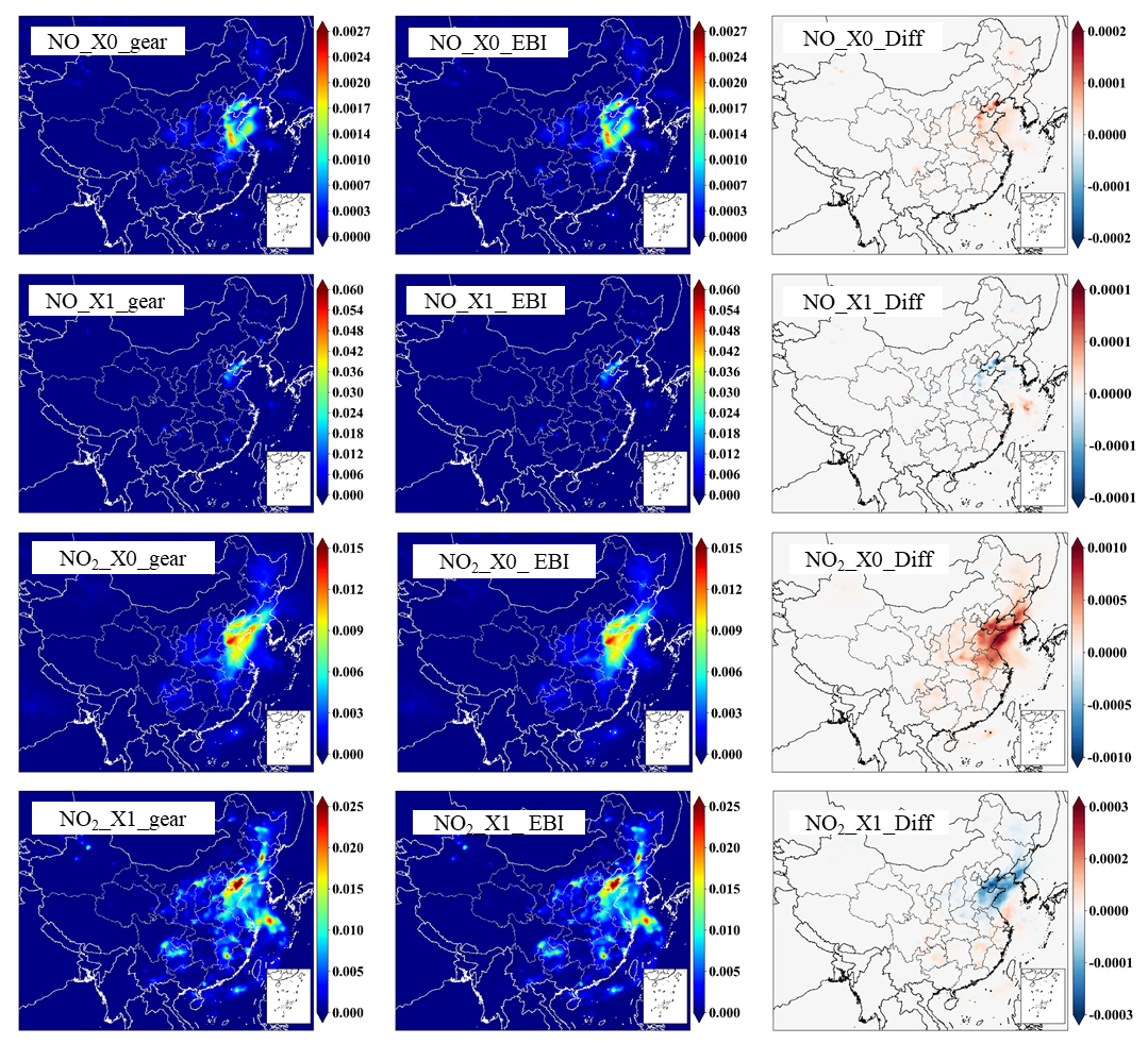
Figure 6 Regional distribution of NO and NO₂ from a day-1 CMAQ simulation with 36 km resolution and meteorological fields from WRFv4.1.4. Units are ppm. Publisher's remark: please note that the above figure contains disputed territories.

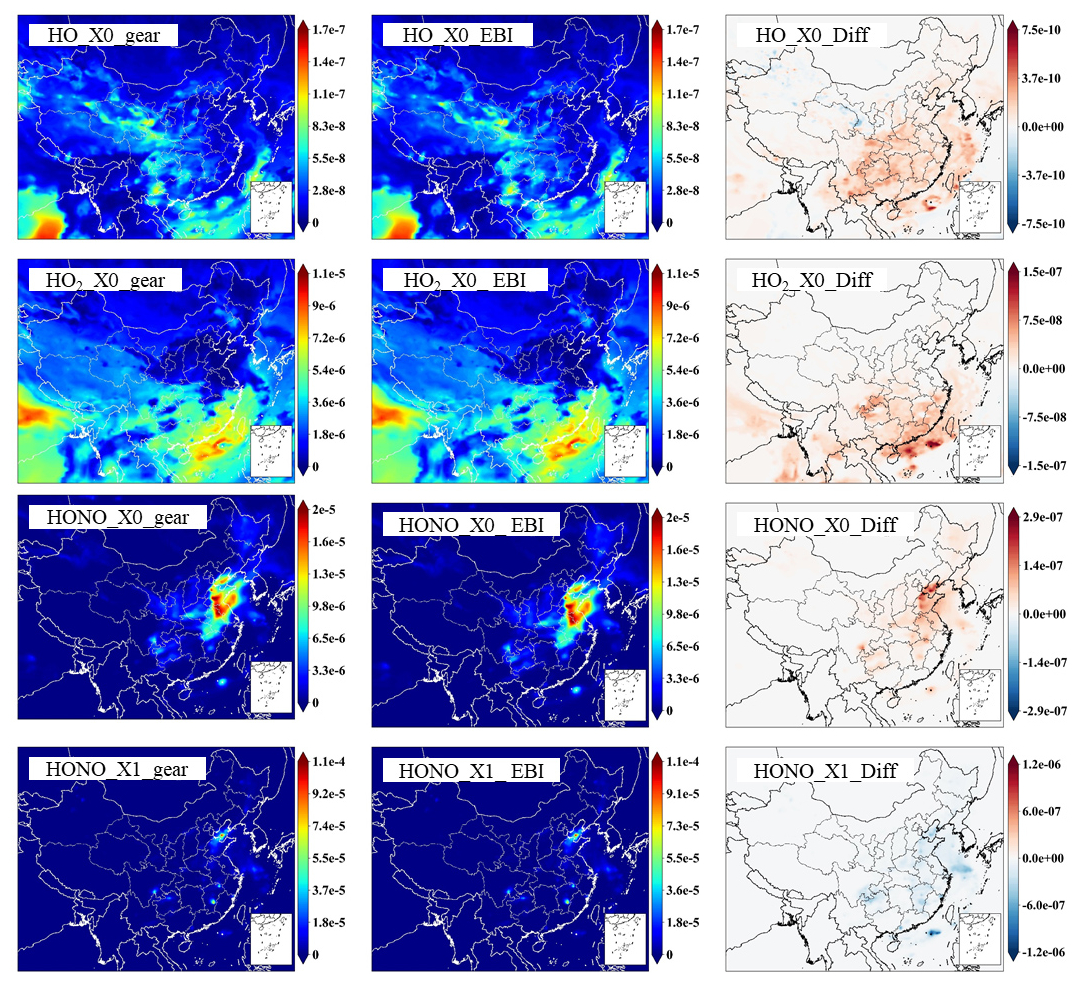
Figure 7 Regional distribution of HO, HO₂, and HONO from a day-1 CMAQ simulation with a 160-row × 130-column, 36 km resolution domain and meteorological fields from WRFv4.1.4. Units are ppm. Publisher's remark: please note that the above figure contains disputed territories.

3.2 Accuracy assessment of the source-oriented EBI solver

The general accuracy of the EBI solver has been tested by Hertel et al. (1993). The accuracy of the proposed source apportionment EBI scheme was evaluated by comparing predicted results with those from SMVGEAR. For this comparison, results from the first day of a 3 d simulation are primarily presented to highlight the maximum potential discrepancy between EBI and SMVGEAR.

Hourly average concentrations of the 3 d NO, NO₂, PAN, HONO, OH, and HO₂ at each grid cell in the surface layer of the 36 km domain were selected as sample species for accuracy evaluation because these are the important species treated by the source-oriented EBI solver. The maximum and mean values of the normalized error of these species are listed in Table 3. For all these species, the maximum normalized error among all grid cells is less than 15 %, and the mean normalized error does not exceed 4 % on the first day. Subsequently, the error gradually decays over the following 2 d, reaching an order of magnitude of 0.1 % to 1 % by the third day. This indicates that the accuracy of the source-oriented EBI scheme is acceptable, as the errors are anticipated to diminish further with increasing flow time.

For OH and HO₂, the EBI solver agrees with the SMVGEAR solver very well, with mean differences of ∼0.19 % and 0.35 %, respectively. This indicates that the overall gas-phase chemistry is not significantly influenced by replacing the SMVGEAR solver with the EBI scheme. Figure 3 shows the comparison of all the hourly concentrations of OH and HO₂ at hour 6, which represent average concentrations between 14:00 and 15:00 local time. The EBI results agree with the SMVGEAR solver results across all concentration ranges that span more than 3 orders of magnitude. Figure 4 shows the comparison of hourly concentrations of NO₂, NO, NO₃, HONO, and PAN for hour 24 of day-1, with the day-2 and day-3 results presented in Figs. A2 and A3, respectively. For the total concentrations of these species (i.e., sum of the concentrations of the source-tagged species), the source-oriented EBI predictions agree very well with the observations. For the individual source-tagged species, differences between the EBI and SMVGEAR results are highest among the NO₂, NO, and HONO species that are used to track the initial and boundary contributions (IC/BC type, first column of Fig. 4). The results shown in the plots are essentially initial concentrations because the boundary conditions for NO and NO₂ are quite low and will not contribute to such high concentrations (see Fig. 6 – the regional NO₂ and NO plots). The source-oriented EBI predictions for IC/BC species are biased high, while those for other tagged species are biased low, compared to those predicted using the Gear solver. The observed discrepancies arise because the dynamic stage solution predicted by the backward Eulerian scheme is generally slower, exhibiting a significant time lag. In this test, the IC/BC species inherited a concentration field from a 7 d non-source-oriented simulation, while the other tagged species started from near-zero concentrations. Consequently, the decay of IC/BC species (with no emission associated) was overestimated, while the accumulation of other tagged species (associated with emissions) was underestimated. These over-predictions are balanced by the general under-predictions of EBI for species associated with emissions, resulting in close agreement in total concentrations. Furthermore, the errors associated with the EBI prediction exhibit a decreasing trend with advancing flow time and diminish to within a tolerable range (on the order of 0.1 %–1 %) by the end of day 3. This phenomenon suggests that species concentrations asymptotically approach a new steady state dictated by external inputs, with emission intensity being the primary factor.

Figure 5 shows the predicted hourly time series of OH, HONO, NO₂, and PAN at five grid cells that represent no emission and low, medium, high, and intense emission conditions, respectively. For HONO, NO₂, and PAN, predicted concentrations are shown for the IC/BC type and the sum of the tagged species for other emission-related types. This again demonstrates that predicted OH from EBI and SMVGEAR agree with each other at all times under all emission conditions. The fraction of initial concentrations to the total concentration decreases as the emission intensity increases, and the difference between EBI and SMVGEAR remains very small.

Figures 6 and 7 illustrate the spatial distribution of daily average concentrations predicted by the two methods. HO, HO₂, and source-tagged NO, NO₂, and HONO of the 36 km grid were selected as sample species, and the results from the proposed EBI scheme are very close to the SMVGEAR results. The concentration of X0 species predicted by the EBI scheme at high concentration is higher than that predicted by Gear; the reason for such slight deviation is mainly the aforementioned time lag in the results of the backward Euler scheme.

4 Conclusions

In this study, the computational efficiency and thus scalability of the source-oriented approach is greatly improved with a new approach of dealing with these dual-tagged-species reactions. The new approach is based on tracking the total concentration of the source-tagged species and reducing the n² number of second-order reactions into 2n pseudo-first-order reactions for a chemical system with n sources. This method preserves individual species' production and loss rates, thus leading to improved computational efficiency because the total number of reactions increases linearly with the source number. Additionally, the Euler backward iterative (EBI) solver has been successfully implemented with respect to the source-oriented mechanism, with an average of absolute relative error below 5 % and an up to 90 % chemistry time reduction in comparison to SMVGEAR. While efficient source-oriented approaches for primary particles are already available to track a large number of sources simultaneously, the efficient approach developed in this study has the potential to track a large number of sources to evaluate their impact on secondary pollutant formation and can be applied in air quality forecasting models that provide source or source-region contribution information for policymakers towards better emission regulations under meteorological conditions that exacerbate pollution.

Appendix A

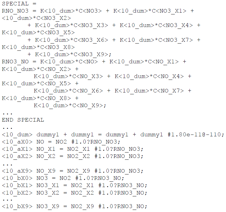
Listing A1 The special reaction rate section (between the keywords SPECIAL and END SPECIAL) and reactions used to implement the source-oriented NO₂+NO₃ reactions in dual-tagged reaction reduction with 10 source types using the chemical mechanism preprocessor CHEMMECH for the CMAQ model. Due to the limitation of the current mechanism preprocessor, a dummy reaction (<10_dum>) is needed so that the original reaction rate can be included in the calculation of the special rate constants. Use of the special rate expression is signaled by including the symbol “?” in the reaction rate coefficient expression.

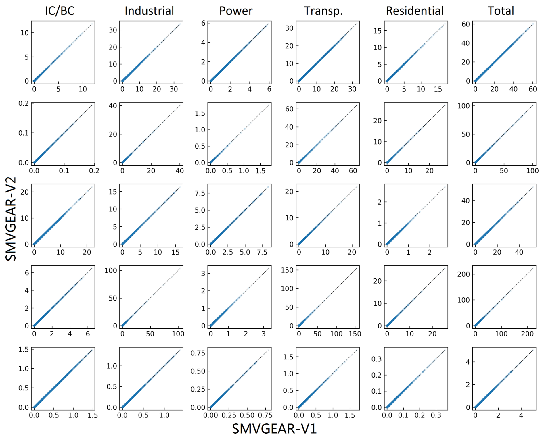
Figure A1 Predicted hourly averaged NO₂, NO, NO₃, HONO, and PAN concentrations for different source types in the last hour of the day-1 simulation using the SMVGEAR solver with the fully expanded source-oriented (V1) and dual-tagged reaction reduction method (V2) mechanism. Concentrations of all grid cells in the surface layer of the 160×130 36 km resolution domain are included in the plot. Concentrations are in units of ppb for NO, NO₂, and PAN and in units of ppt for NO₃ and HONO.

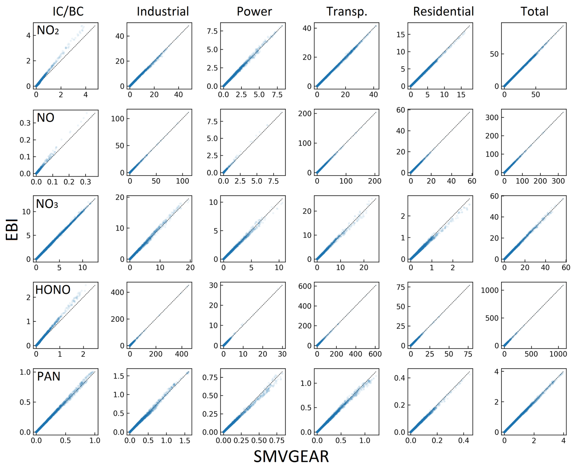
Figure A2 Predicted hourly averaged NO₂, NO, NO₃, HONO, and PAN concentrations for different source types in the last hour of the day-2 simulation using the source-oriented EBI (new) and SMVGEAR (baseline) solvers. Concentrations of all grid cells in the surface layer of the 160×130 36 km resolution domain are included in the plot. Concentrations are in units of ppb for NO, NO₂, and PAN and in units of ppt for NO₃ and HONO.

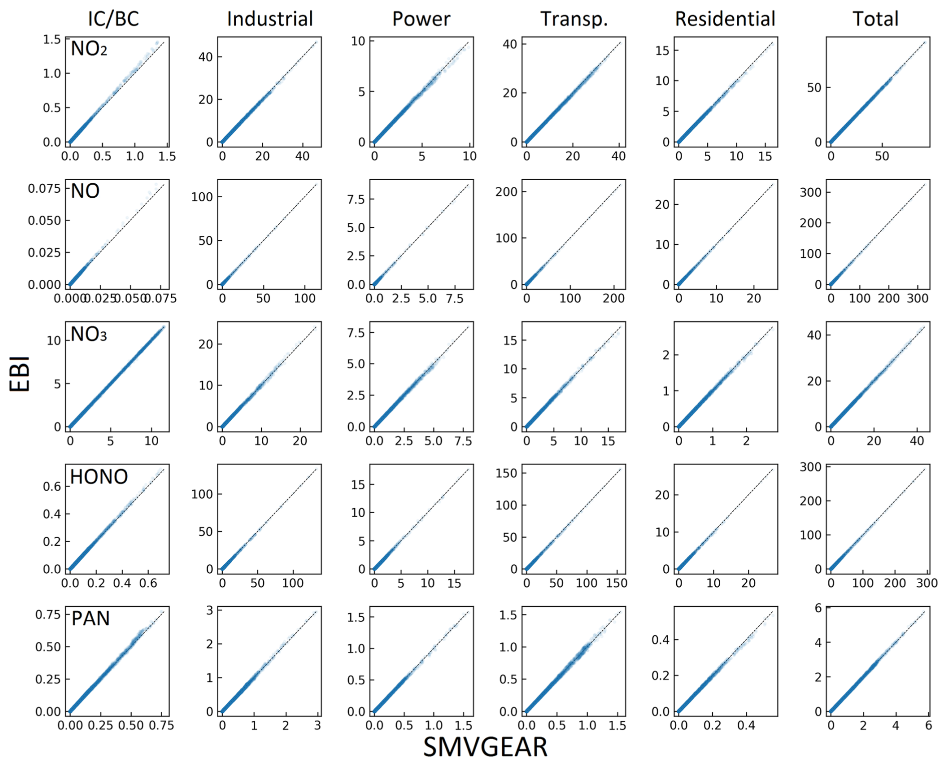
Figure A3 Predicted hourly averaged NO₂, NO, NO₃, HONO, and PAN concentrations for different source types in the last hour of the day-3 simulation using the source-oriented EBI (new) and SMVGEAR (baseline) solvers. Concentrations of all grid cells in the surface layer of the 160×130 36 km resolution domain are included in the plot. Concentrations are in units of ppb for NO, NO₂, and PAN and in units of ppt for NO₃ and HONO.