Disentangling the chemistry and transport impacts of the quasi-biennial oscillation on stratospheric ozone

The quasi-biennial oscillation (QBO) in tropical winds perturbs stratospheric ozone throughout much of the atmosphere via changes in transport of ozone and other trace gases, as well as via temperature changes, both of which alter ozone chemistry. Attributing these causes of QBO–ozone variability may provide insights into model-to-model differences that contribute to ozone simulation. Here we develop a novel metric of steady-state ozone (SSO) to separate these effects: SSO calculates the local steady-state response of ozone due to the changes in temperature, chemical species, and overhead ozone column; the response due to circulation change is presumed when SSO shows no response. It is applied to the nudged Department of Energy's Energy Exascale Earth System Model version 2 (E3SMv2) with interactive ozone chemistry to demonstrate its validity. The E3SMv2 simulations nudged to reanalysis data produced reasonable wind and ozone patterns, especially in the tropics. Consistent with previous studies, we find clear demarcations with pressure. Ozone perturbations in the upper stratosphere (<6 hPa) are predicted by temperature changes; those between 6 and 20 hPa are predicted by NO_y changes, and those in the lower stratosphere show no temperature or NO_y response and are presumably driven by circulation changes. These results are important for diagnosing model-to-model discrepancy in QBO–ozone response and enhancing the reliability of ozone projections.

1 Introduction

The quasi-biennial oscillation (QBO) is the principal mode of dynamical variability in the stratosphere. It is the key source of interannual variability in the overall chemical composition of the stratosphere (Randel et al., 1998; Shuckburgh et al., 2001; Park et al., 2017), manifesting primarily through ozone (Reed, 1964; Bowman, 1989; Wang et al., 2022).

The QBO affects ozone through both transport via atmospheric circulation and chemical processes via the changed composition of the atmosphere (Reed, 1964; Holton, 1989; Gray and Dunkerton, 1990; Chipperfield and Gray, 1992; Chipperfield et al., 1994; Politowicz and Hitchman, 1997; Jones et al., 1998; Baldwin et al., 2001). The alternate change in QBO phase speeds up and slows down the vertical ascent in the tropics, which pushes the ozone profile up and down; the QBO temperature warms and cools the stratosphere, which accelerates and decelerates the ozone cycle; and QBO-associated vertical transport of trace gases, such as a reactive nitrogen reservoir NO_y, may also affect the ozone cycle.

Disentangling these causes of QBO–ozone variability is useful for understanding model-to-model discrepancies in QBO–ozone simulations, which in turn contributes to improved ozone projections, such as the rate of ozone recovery, which is still accompanied by large uncertainties due to internal climate variabilities like the QBO (Chipperfield et al., 2017; Stone et al., 2018). Yet, the role of chemical and dynamical processes in QBO–ozone variability is still under debate (Zhang et al., 2021). Ling and London (1986) pointed to a close relationship between ozone and QBO-induced temperature anomalies and their associated photochemistry above 15 hPa. Chipperfield et al. (1994) and Tian et al. (2006) attribute the QBO–ozone relationship to QBO modulation of NO_y species rather than temperature changes above 10–15 hPa. Butchart et al. (2003), on the other hand, used a 3-D chemistry–climate model to argue that transport is just as important above 15–20 hPa. Currently, challenges in attributing QBO–ozone variability remain due to the co-existence of chemistry and transport impacts (Baldwin et al., 2001) and model limitations in simulating free-running QBO variability (Richter et al., 2020), including asymmetries between QBO phases – namely a stronger and shorter QBO easterly phase and a weaker and longer QBO westerly phase (Scaife et al., 2014; Richter et al., 2020). To separate the co-existing impacts, we built upon a novel use of the steady-state ozone (SSO) metric derived from linearized stratospheric ozone chemistry (Linoz; McLinden et al., 2000; Hsu and Prather, 2009). The SSO assumes a steady state of ozone chemistry in the stratosphere and is calculated in the absence of dynamics, thereby isolating the impacts due to chemical reactions and those due to temperature perturbations. The determination of transport-driven ozone is then based on the difference in modeled ozone from the steady-state ozone. Studies have shown the validity of using linearized chemistry to represent ozone (McLinden et al., 2000) and ozone's response to 4×CO₂ (Meraner et al., 2020), and our study builds on this. Current state-of-the-art Earth system models still have problems in simulating a realistic QBO. To date, only 15 of the 30 models in the Coupled Model Intercomparison Project phase 6 (CMIP6) include an internally generated QBO (Richter et al., 2020). Within these models, the simulated QBO amplitudes and periods often fail to match those of the observed pattern. The World Climate Research Programme (WCRP) Atmospheric Processes And their Role in Climate (APARC) project started a QBO initiative (QBOi) in 2015 to improve chemistry–climate model (CCM) simulations of tropical variability (Butchart et al., 2018). Phase II of QBOi includes a set of nudging experiments to examine the QBO's impact on climate, and here we build on those experiments.

In this study, we use the newly developed SSO metric on experiments following the QBOi phase II protocol to disentangle the chemical and transport impacts of QBO on ozone. Our primary modeling tool is the Department of Energy (DOE) Energy Exascale Earth System Model version 2 (E3SMv2; Golaz et al., 2022) with interactive stratospheric ozone (Linoz v2 and Linoz v3; McLinden et al., 2000; Hsu and Prather, 2009), and we secondarily examine certain QBOi experiments from the National Center for Atmospheric Research (NCAR) Community Earth System Model (CESM). We also develop a new index of the QBO phase using a nonlinear principal component analysis (NLPCA) of tropical zonal winds, which better retains the asymmetric patterns of the QBO than the standard linear PCA QBO index (Wallace et al., 1993). Phase-based composite diagrams are then created to investigate the temporal evolution of ozone patterns, both observed and modeled. We show that the SSO is a novel and effective tool for separating the chemical and transport processes associated with the QBO's effect on ozone, and it may be applied to diagnose the model-to-model discrepancies in QBO–ozone response. The observational data and ozone modeling, the NLPCA method, and the SSO are described in Sect. 2. The results are given in Sect. 3. The discussion and conclusions are summarized in Sect. 4.

2 Data and methods

2.1 CCM models

The primary model for this study is E3SMv2. E3SM's atmospheric component (EAMv2) is run here as a CCM with specified sea surface temperatures (SSTs) and has 72 vertical layers and a horizontal resolution of about 100 km. Following Richter et al. (2019), EAMv2 employs gravity wave (GW) parameterizations that include orographic GWs (McFarlane, 1987), convective GWs (Beres et al., 2004), and GWs generated by frontal systems (Charron and Manzini, 2002). Tunable parameters in the orographic and frontal GW parameterizations remain the same as in EAMv1 (Xie et al., 2018; Rasch et al., 2019). The tunable parameters in convective GWs were explored to produce a more realistic QBO in EAMv1 with a period of around 27 months, which is much closer to observations (28 months) compared to 16 months in the default EAMv1 (Richter et al., 2019). Nevertheless, the modeled QBO remains weak in amplitude. Stratospheric ozone in E3SMv2 is calculated interactively through transport and the chemical Linoz module (McLinden et al., 2000; Hsu and Prather, 2009), which was updated from the E3SM O3v1 to O3v2 module (Tang et al., 2021). Linoz v2 data tables are used to calculate the 24 h average ozone tendency (i.e., net production minus loss) from an adopted climatological mean state for key species (CH₄, H₂O, NO_y, Cl_y, Br_y) and first-order Taylor series expansions of the local ozone, temperature, and overhead ozone column (see Eq. 3 in Sect. 4.1). The data tables are generated for each year assuming key chemical species and families (CH₄, H₂O, NO_y, Cl_y, Br_y) follow monthly zonal mean climatologies that scale with the slowly varying changes in the tropospheric mean abundance of their source gases (e.g., N₂O, CFCs, halons, CH₄, tropopause H₂O). The Linoz model produces a reasonable stratospheric ozone climatology, including seasonal and interannual variability and the Antarctic ozone hole (Tang et al., 2021; Ruiz and Prather, 2022). The tropospheric chemical package for E3SMv2 (chemUCI) was not used, and the lower boundary for Linoz was set to 30 ppb. Thus, none of the ozone column variability arises from tropospheric ozone chemistry. E3SMv2 diagnostics on the tendency of tropospheric ozone calculate a geographically resolved stratosphere–troposphere exchange (STE) flux of ozone at every time step (Hsu et al., 2005; Tang et al., 2013).

The secondary model for this study is CESM2 (Emmons et al., 2020), using a modified version of the Community Atmosphere Model (CAM) with 83 vertical levels (Randall et al., 2023), which is run here as a CCM with specified sea surface temperatures (SSTs). CAM uses a finite-volume dynamical core with a nominal 1° horizontal resolution and with physics from the Whole Atmosphere Community Climate Model version 6 (WACCM6; Gettelman et al., 2019). The parameters for the convective GW momentum transport scheme are tuned specially for this version to obtain a realistic, naturally generated QBO (Randall et al., 2023). The inline ozone calculation in CESM2 is replaced with a monthly mean 3-D ozone climatology specified from a previous WACCM simulation. This input ozone forcing is formed by merging WACCM simulations for historical (1850–2014, three members) and future periods (2015–2100, one member). As the mean of free-running CCM simulations, this ozone input climatology does not have any significant QBO-like variability, and thus it cannot trigger a QBO in the CCM (Butchart et al., 2023).

Both models are run with tropical winds being nudged to the observations, and hence the synchronicity of the QBO should be similar, and we can thus compare them directly with observations. With the CESM2 QBO simulation, we must limit our analysis to examining the forced dynamical response (temperature, circulation), but with E3SM results we can compare the modeled QBO–ozone interactions with observations.

2.2 Observed ozone and wind

For ozone, we derive the observed QBO signal from the monthly zonal mean total column ozone (TCO) using Multi-Sensor Reanalysis version 2 (MSRv2) data (van der A, et al., 2015). This latitude-by-month dataset initially covers the 1979–2012 period and is later extended to 2020. For stratospheric profiles, we use the zonal monthly mean latitude-by-altitude dataset from the Concentration Monthly Zonal Mean (CMZM) product (Sofieva et al., 2023). This altitude-by-month profile dataset covers the period of 1985–2020. The vertical levels are converted to pressure levels, inverting the pressure–altitude formula, $z^{*}=\mathrm{16}{\log }_{\mathrm{10}}(\mathrm{1000}/P)\mathrm{km}$. We compared these ozone data with the overlapping period from microwave limb sounder (MLS) data (v5 level 3, Schwartz et al., 2021) and found only small differences with regard to QBO patterns.

We use ERA5 data (wind, temperature, geopotential height) from the reanalysis produced by the European Centre for Medium-Range Weather Forecasts (ECMWF) Integrated Forecasting System (Hersbach et al., 2020). The version we use has 137 hybrid sigma model levels from the surface to the model top at 0.01 hPa, and the horizontal resolution is about 31 km. We use monthly mean data for the period of 1979–2020 to analyze QBO-related dynamical changes and 6-hourly ERA5 tropical zonal wind (15° N–15° S) to nudge the model simulations mentioned below. We use the 5° S–5° N tropical average zonal wind from ERA5 and simulations to determine the QBO phase index. The combined station zonal wind data from the Freie University of Berlin (Naujokat, 1986) for the period of 1979–2020 are also used.

2.3 The QBOi simulations

We use two experiments from the protocol for phase 2 of QBOi (Butchart et al., 2018; Bushell et al., 2020; Richter et al., 2020):

1. Exp1-ObsQBO (E3SMv2 nudged). The zonal wind in the tropical stratosphere is constrained to follow the observed QBO evolution by nudging it toward ERA5 reanalysis (Hitchcock et al., 2022). Thus, the stratospheric climate, including temperature and circulation in the tropics, is constrained.

2. Exp1-AMIP (E3SMv2 natural). The zonal wind in the tropical stratosphere evolves freely in each CCM, being forced only by SSTs and trace gas radiative forcing; there is no nudging. The SSTs are historical and include interannual variability, primarily from the El Niño–Southern Oscillation (ENSO).

The nudging is applied to the zonal wind over the range 8–80 hPa and 15° S–15° N (Fig. S1 in the Supplement – nudging coefficient shown is for E3SMv2; that for CESM2 is similar). There is a slight difference in how the models were nudged: E3SMv2 is nudged to the “full-field” ERA5 wind field, including the longitudinal variability, while CESM2 is nudged to the zonally averaged ERA5 zonal wind field. The nudging relaxation timescale is 5 d. The current setup forces the models to match the tropical QBO dynamic variability while allowing other variabilities to evolve freely (e.g., semi-annual oscillation). For each experiment we produced three ensemble members, and the ensemble mean is used for analysis.

To better understand the QBO–chemistry interactions, we performed two additional nudged single-ensemble 1979–2020 runs with E3SMv2 using different chemical models: one with an expanded stratospheric chemistry, Linoz v3 (referred to as E3SMv2 Linoz v3 nudged; Hsu and Prather, 2010), which calculates NO_y–N₂O–CH₄–H₂O as prognostic tracers and includes their interactions with ozone, and a second with fixed-ozone climatology as prescribed for CESM2 (E3SMv2 fixed-ozone nudged).

2.4 NLPCA of QBO phase

To build a timeline composite picture of the QBO in any variable, we need to define the phases of each QBO and align these phases over a 28-month period. Phase asymmetry and nonlinear features of the evolution of the QBO phase are found in many studies (Lindzen and Holton, 1968; Holton and Lindzen, 1972; Giorgetta et al., 2002). The most obvious and sharply defined synchronization point is when the QBO west phase (QBOw; i.e., prevailing westerlies) transitions to the east phase (QBOe; prevailing easterlies) at some pressure level in the middle stratosphere (taken as 10 hPa here) (Naujokat, 1986; Pahlavan et al., 2021a, b; Kang et al., 2022). The QBOe phase is typically longer (e.g., Bushell et al., 2020), with wind speeds about twice as strong as those of the QBOw (Naujokat et al., 1986; Kang et al., 2022). The problem with defining the QBO phase (index) simply as the month-to-month difference relative to the synchronization point (e.g., Ruiz et al., 2021) is that the duration of different phases varies across successive QBOs.

Previous use of PCA-derived QBO indices (Wallace et al., 1993) did not allow for this asymmetric and nonlinear behavior. Lu et al. (2009) noted that the reconstructed wind series from the PCA looked more sinusoidal in time than the actual winds, and thus the asymmetries between phases did not show up in the PCA-based indices. To address these issues, we use an NLPCA method that utilizes a hierarchical-type neural network with an auto-associative architecture (Scholz and Vigário, 2002). It is a nonlinear generalization of the standard PCA from straight lines to curves in the original data space and a natural extension to the PCA method by forcing the nonlinear components to the same hierarchical order as in the standard PCA (Scholz and Vigário, 2002). The NLPCA model described here has five layers with three hidden layers of neurons. The layers of the neural network for NLPCA follow the sequence input–encoding–bottleneck–decoding–output, with a structure of $n-(\mathrm{2}k+\mathrm{2})-k-(\mathrm{2}k+\mathrm{2})-n$, where n refers to the dimension of the input/output dataset, and k is the number of dimensions for the bottleneck layer. To achieve robustness, the NLPCA is applied to the tropical zonal wind data (5° S–5° N; 10–70 hPa) for a set of k varying from 2 to 5, with 100 runs (different in random initialization weights) for each k. The optimal number of k is set as 5 as it gives the lowest root-mean-square error between the input and output. The comparisons of QBO phase angles and QBO transition points are shown in Fig. S2a and b. It is shown that the first and second principal components (PC1 and PC2) of the NLPCA account for approximately 90 % of the whole variance (Fig. S2c and d).

Following previous studies (Wallace et al., 1993; Hamilton and Hsieh, 2002; Lu et al., 2009), the QBO phase index ψ is calculated using PC1 and PC2 as follows:

$$\begin{array}{}\text{(1)}& \mathit{\psi }=\arctan (v/u)(-\mathit{\pi }\le \mathit{\psi }\le \mathit{\pi }),\end{array}$$

where u and v are the time series of PC1 and PC2, respectively. The positive and negative phase angle index ψ corresponds to QBOw and QBOe, respectively.

We compare the reconstructed zonal wind anomalies using NLPCA and PCA (Wallace et al., 1993) with the QBO cycle in the observation (Fig. 1). It is shown that the observed QBO transition corresponds to an abrupt downward propagation in QBOw and a slower downward transition in QBOe (indicated by clustering points from B to C to A in the black triangular shape in Fig. 1a). The NLPCA captures a large part of this sharp transition in QBOw, while PCA underestimates it (indicated by points near C in Fig. 1a). This difference is also clearly shown in a typical QBO cycle of September 1970–March 1972 (Fig. 1b–d, black arrows exhibit the downward propagation in QBOw) and the time series of the NLPCA/PCA QBO phase (index) (Fig. S2).

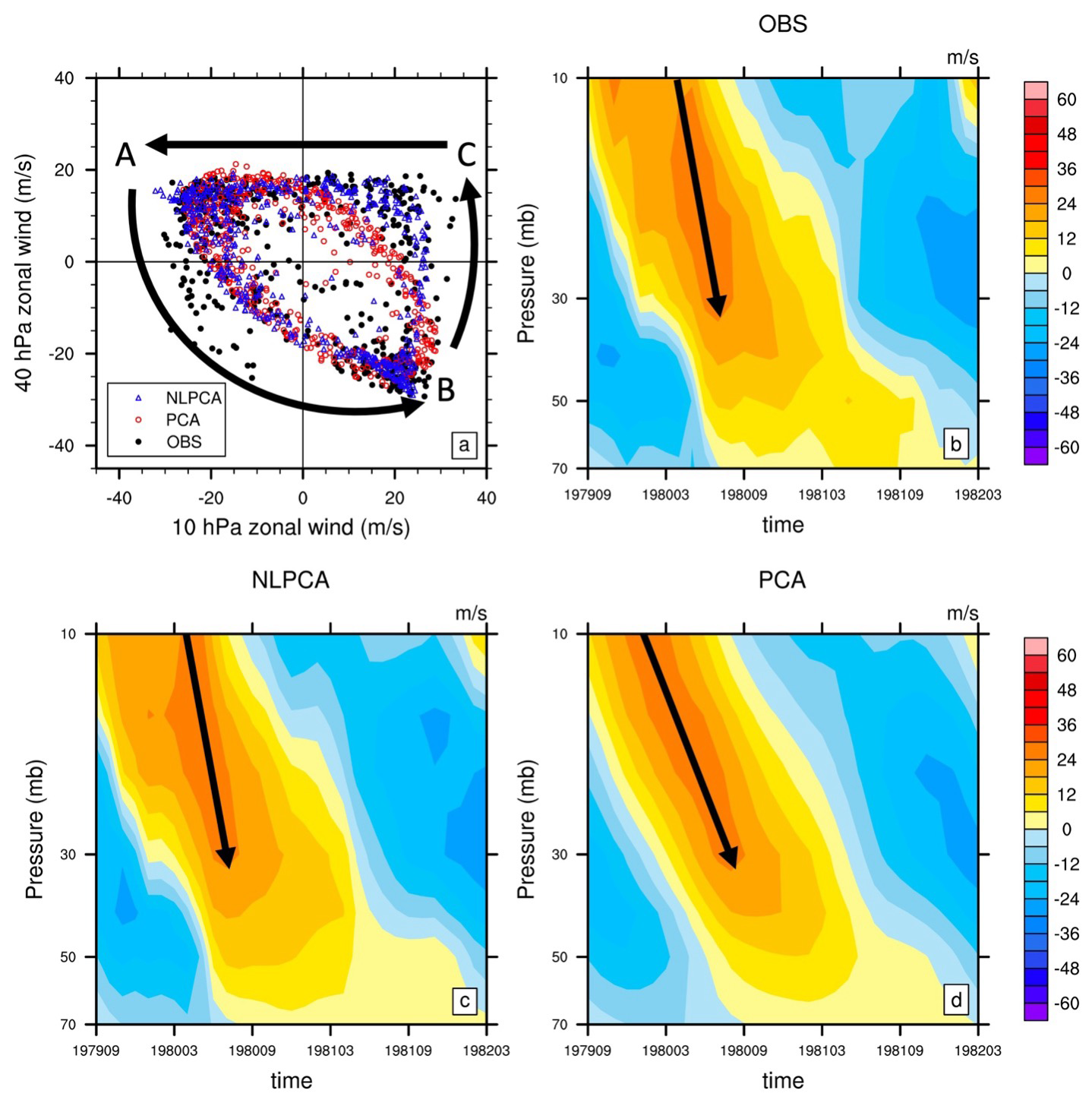
Figure 1 (a) Scatterplot of 1979–2020 monthly mean zonal wind anomaly (m s⁻¹) at 10 vs. 40 hPa for observations (black), the NLPCA reconstruction (blue), and the PCA reconstruction (red). Typical cycle of QBO (September 1979–March 1982) from (b) observational station data from the University of Berlin, (c) the NLPCA reconstruction, and (d) the PCA reconstruction.

The NLPCA-derived QBO index is more realistic in following the atmospheric changes; therefore, it is impractical to map the NLPCA phases onto the monthly mean model diagnostics. Thus, our QBO composites use simple monthly time steps around our best synchronization point, which, from the NLPCA, we take to be at the transition where phase angle index ψ crosses 0, with negative values before and positive values after it (from the QBO easterly to the QBO westerly phase). It is demonstrated that, compared to QBO composites produced using the PCA-derived QBO index, those that are produced using the NLPCA-derived index show a shifted QBO synchronization month (Fig. S2b). This results in a larger contrast in observed tropical zonal wind anomalies between QBOw and QBOe (Fig. S3a and b) that is consistent with contrasts described in previous literature (Hamilton and Hsieh, 2002; Lu et al., 2009). This larger contrast between NLPCA and PCA in zonal wind anomalies corresponds with the larger contrast in the total column ozone anomalies (Fig. S3c and d).

2.5 Linoz calculation of steady-state ozone

To examine the chemical ozone response to the QBO, we use the SSO calculated from both Linoz v2 and Linoz v3 models. For Linoz v2, this metric calculates the local SSO response of ozone to the modeled changes in temperature, chemical species, and overhead ozone column; for Linoz v3, more long-lived species are added. For Linoz v2, the SSO is derived from Eq. (4) of McLinden et al. (2000). The photochemical SSO mole fraction f_ss (parts per million, moles per mole of dry air) is expressed as follows:

$$\begin{array}{}\text{(2)}& \begin{array}{rl}{f}^{\text{ss}}=f^{\mathrm{o}}+[& (P-L{)}^{\mathrm{o}}+{\displaystyle \frac{\partial (P-L)}{\partial T}}{\mathrm{|}}^{\mathrm{o}}(T-T^{\mathrm{o}})\\ & +{\displaystyle \frac{\partial (P-L)}{\partial C_{{\mathrm{O}}_{\mathrm{3}}}}}{\mathrm{|}}^{\mathrm{o}}(C_{{\mathrm{O}}_{\mathrm{3}}}-C_{{\mathrm{O}}_{\mathrm{3}}}^{\mathrm{o}})]\mathit{\tau }.\end{array}\end{array}$$

This is derived by setting $\frac{d(P-L)}{dt}=\mathrm{0}$ for Eq. (1) as in McLinden et al. (2000). The values f^o, T^o, and $C_{{\mathrm{O}}_{\mathrm{3}}}^{\mathrm{o}}$ are the climatological values of the local ozone, temperature, and overhead column ozone tables used to calculate the Linoz tendencies. (P−L)_o is the ozone net production minus loss tendency, and the partial derivatives are the sensitivity of the net production to temperature and overhead column ozone.

A major assumption of Linoz v2 here is that the key chemical families (NO_y, Cl_y, Br_y) and long-lived reactive gases (N₂O, CH₄, H₂O) do not change from their climatological values used to generate the tables (Hsu and Prather, 2009). This steady-state calculation ignores transport tendencies and are thus applied only where the photochemistry is rapid; i.e., $\mathit{\tau }=-[\frac{\partial (P-L)}{\partial f}{\mathrm{|}}_{\mathrm{o}}{]}^{-\mathrm{1}}<\mathrm{100}\mathrm{d}$. Figure 2 shows this Linoz v2 steady-state calculation (f_SS, T, τ) for January and July using ERA5 monthly mean temperature.

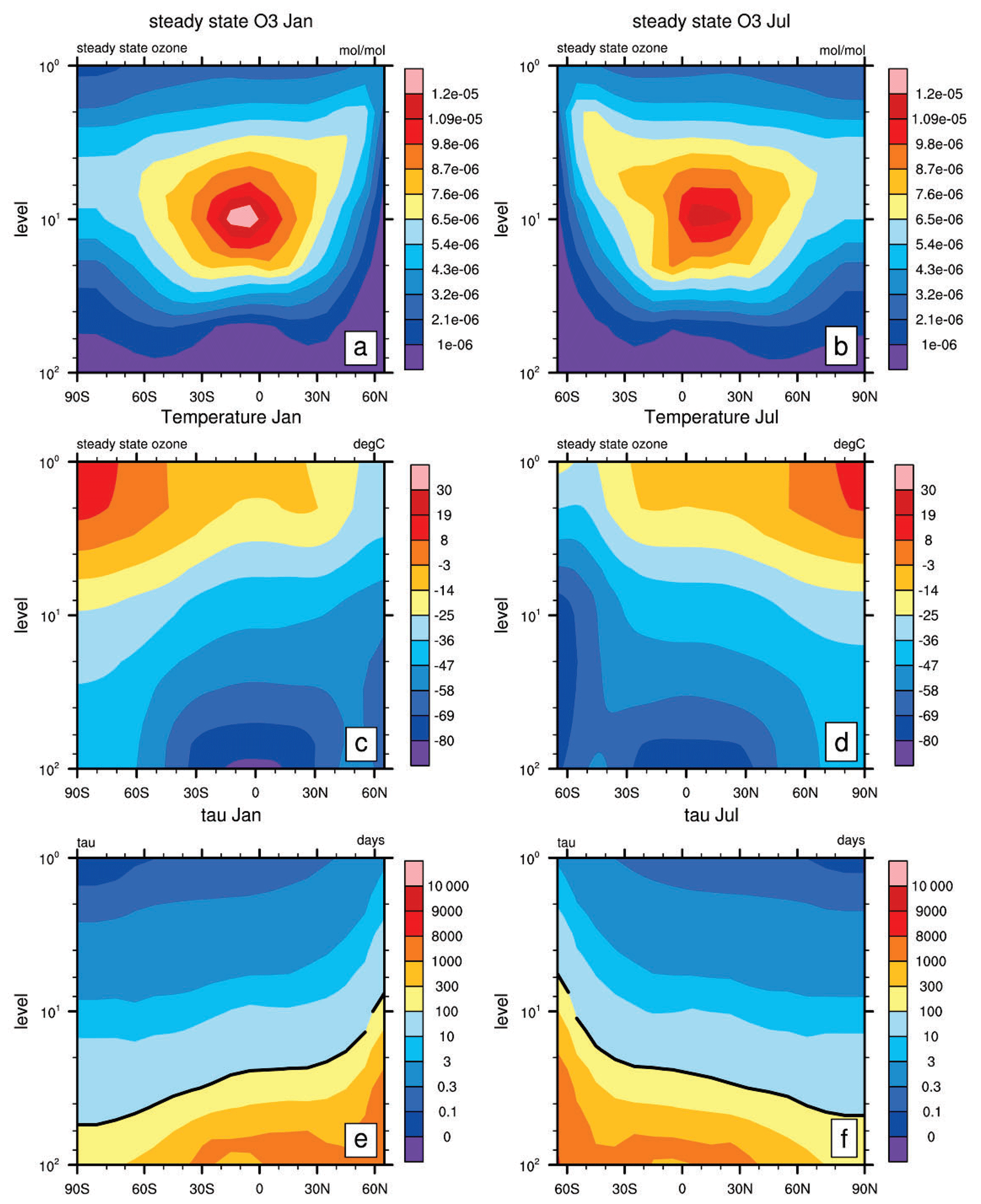
Figure 2 The (a, b) steady-state ozone (mol mol⁻¹) derived using Linoz v2 for E3SMv2 temperature, (c, d) ERA5 temperature (°C), and (e, f) photochemical relaxation time τ (days) in January and July. The thick black line in (c, d) denotes the 300 value line.

An alternative version (Linoz v3) of the SSO derived from Hsu and Prather (2010) is expressed as follows:

$$\begin{array}{}\text{(3)}& \begin{array}{rl}{f}_{\text{ss}}=f_{\mathrm{o}}+[& (P-L{)}_{\mathrm{o}}+{\displaystyle \frac{\partial (P-L)}{\partial T}}{\mathrm{|}}_{\mathrm{o}}(T-T_{\mathrm{o}})\\ & +{\displaystyle \frac{\partial (P-L)}{\partial C_{{\mathrm{O}}_{\mathrm{3}}}}}{\mathrm{|}}_{\mathrm{o}}(C_{{\mathrm{O}}_{\mathrm{3}}}-C_{{\mathrm{O}}_{\mathrm{3}}}^{\mathrm{o}})\\ & +{\sum }_{j=\mathrm{1}}^{j=\mathrm{5}}{\displaystyle \frac{\partial (P-L)}{\partial f_j}}{\mathrm{|}}_{\mathrm{o}}(f_j-f_j^{\mathrm{o}})]\mathit{\tau }.\end{array}\end{array}$$

This is similar to Eq. (2), except it includes the contribution from sources of $f_{{\mathrm{N}}_{\mathrm{2}}\mathrm{O}}$, $f_{{\mathrm{NO}}_y}$, $f_{{\mathrm{CH}}_{\mathrm{4}}}$, and $f_{{\mathrm{H}}_{\mathrm{2}}\mathrm{O}}$. This may be used to provide a more precise diagnosis of the SSO from models that have outputs of these chemistry species in addition to the temperature profile.

3 Impact of QBO on circulation and stratospheric ozone

Nudging the tropical zonal wind creates QBO-driven perturbations to the temperature and residual circulation that we can diagnose in both the E3SMv2 and the CESM2 runs and compare with observations. For E3SMv2 with interactive ozone, we are able to see the changes in ozone. This also applies to the simulations with an internally generated QBO.

We create a similar composite of the QBO cycle using E3SMv2/CESM2 following Ruiz et al. (2021) to see the full QBO cycle influence on stratospheric ozone. The time composite is created for each month starting 14 months prior to and extending 14 months after the QBO transition for 1979–2020. The center of the composite is when the NLPCA-derived QBO phase angle index (see Sect. 2.4) shifts from negative to positive (QBOe → QBOw). We create composites for circulation (zonal wind, temperature, and residual circulation) and chemistry tracers (total column ozone (TCO), ozone concentration, NO_y) as a function of QBO phase. For TCO, we calculate the zonal mean averages to produce the global map of composites; for all other fields, we process the tropical (15° S–15° N) and extratropical (30–60° S, 30–60° N) vertical profiles of the regional average using latitudinal weight to produce the composites. The CESM2 ozone composite is not shown since its ozone is prescribed.

The structure of this section is as follows. We first analyze the impact of nudged QBO on circulation in E3SM and CESM in Sect. 3.1. Following this, we analyze its impact on global TCO and tropical/extratropical ozone in Sects. 3.2 and 3.3. The chemistry and transport impacts of QBO are further analyzed using the SSO metric in Sect. 3.4. The overall performances of the models are summarized in Sect. 3.5.

3.1 Impact of QBO on circulation

In this section, we examine the impact of nudged QBO on circulation in both E3SMv2 and CESM2. We first analyze its impact on zonal wind and subsequently on temperature and residual circulation (e.g., ${\underset{\mathrm{¯}}{w}}^{\ast }$, which characterizes the transport impact of the Brewer–Dobson circulation).

Through nudging, the anomalous tropical zonal winds (15° S–15° N) in nudged E3SMv2 and CESM2 simulations exhibit a similar negative–positive–negative pattern to that of ERA5 from QBOe to QBOw (Fig. 3). In terms of the magnitude, E3SMv2's zonal wind pattern above 6 hPa is slightly stronger than that of ERA5 and CESM2. Despite this minor difference, both models generally reproduce the QBO signal in the tropical nudging regions. Corresponding to the zonal wind changes shown in Fig. 3, the tropical temperature (Fig. 4a–c) in both models exhibits a negative–positive–negative–positive pattern, similar to that of ERA5. Also shown is the residual vertical transport ${\underset{\mathrm{¯}}{w}}^{\ast }$ that exhibits a positive–negative–positive–negative pattern, similar to that of ERA5 (Fig. 4d–f). Studies have shown that QBOe tends to relate to cooling and upward advection, while QBOw relates to warming and downward advection (Baldwin et al., 2001). The tropical temperature and ${\underset{\mathrm{¯}}{w}}^{\ast }$ results are thus in phase with zonal wind change in both models.

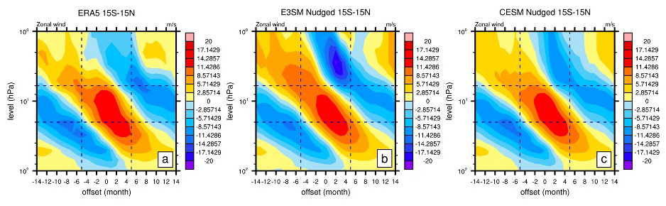
Figure 3 Pressure–time cross-section of the tropical (15° S–15° N) zonal wind anomaly (m s⁻¹) as a function of the QBO phase for (a, d) ERA5, (b, e) E3SMv2, and (c, f) CESM2 for 1979–2020. Here, 0 is centered on the month when the QBO index shifts from QBOe to QBOw (determined by when the current QBO index <0 and the next QBO index >0). The QBO phase is determined by the 5° S–5° N average of the zonal wind.

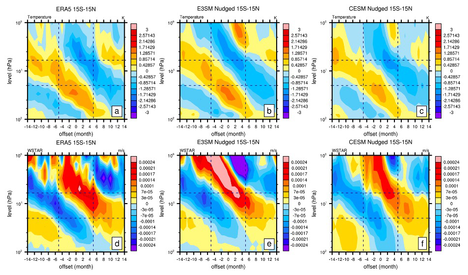
Figure 4 Pressure–time cross-section of the tropical (15° S–15° N) temperature (K) and ${\underset{\mathrm{¯}}{w}}^{\ast }$ anomaly (transformed Eulerian mean residual vertical transport, m s⁻¹) as a function of the QBO phase for (a, d) ERA5, (b, e) E3SMv2, and (c, f) CESM2 for 1979–2020. Here, 0 is centered on the month when the QBO index shifts from QBOe to QBOw (determined by when the current QBO index <0 and the next QBO index >0). The QBO phase is determined by the 5° S–5° N average of the zonal wind.

In the extratropical region (30–60° N, 30–60° S), the results for the zonal wind are noisier (Fig. S4). The ERA5 results exhibit scattered signals of zonal wind changes for both hemispheres (Fig. S4a). The two models exhibit noisy results like those of ERA5, with CESM2 being closer to ERA5. This is expected since the extratropics are more likely to be affected by dynamic noise from the polar regions. Unlike the results of the zonal wind, the temperature and residual vertical transport ${\underset{\mathrm{¯}}{w}}^{\ast }$ results are smoother for both observations and nudged simulations. It is shown that ERA5 exhibits about two cycles of a positive–negative phase shift for temperature (Fig. 5a and d) and a negative–positive phase shift for ${\underset{\mathrm{¯}}{w}}^{\ast }$ (Fig. 6a and d) from QBOe to QBOw, although the Southern Hemisphere (SH) is noisier than the Northern Hemisphere (NH). Both models seem to have better agreement with ERA5 in the NH (Figs. 5b and c and 6b and c), while E3SMv2 performs better than CESM2 in the SH (Figs. 5e and f and 6e and f). Studies have shown that the QBO signal in extratropical temperature and vertical advection is at an approximately 180° phase shift relative to the tropical QBO signal (Baldwin et al., 2001). The results shown here are in phase with our nudged QBO signal in the tropics. Overall, the two models show some signs of QBO-related signals outside of the regions of nudging on temperature and ${\underset{\mathrm{¯}}{w}}^{\ast }$, exhibiting the “spillover” effect of QBO nudging.

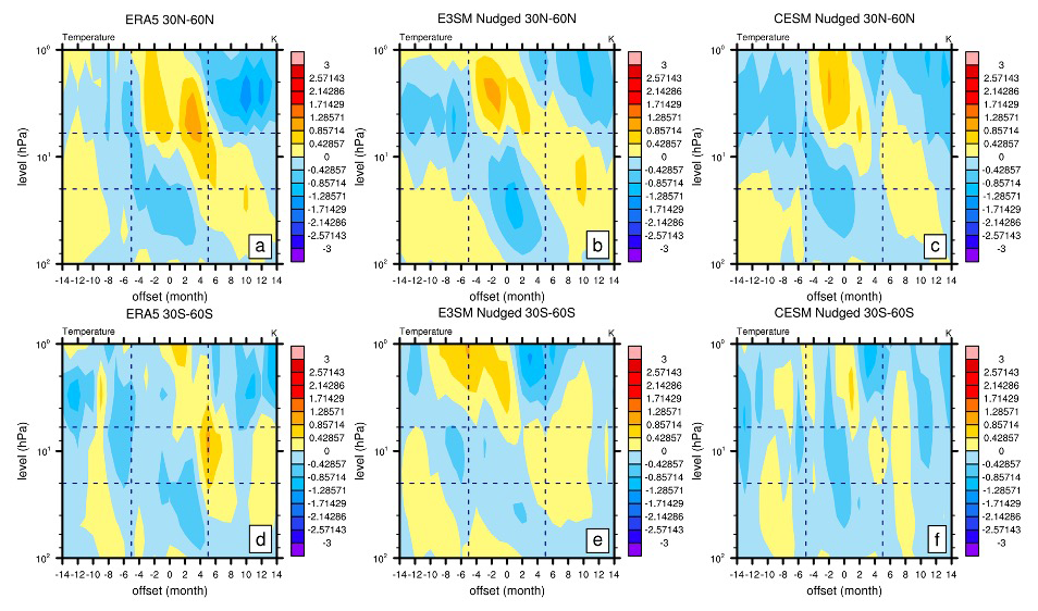
Figure 5 As in Fig. 4 but for the extratropical (30–60° N, 30–60° S) temperature anomaly (K) as a function of the QBO phase for (a, d) ERA5, (b, e) E3SMv2, and (c, f) CESM2 for 1979–2020.

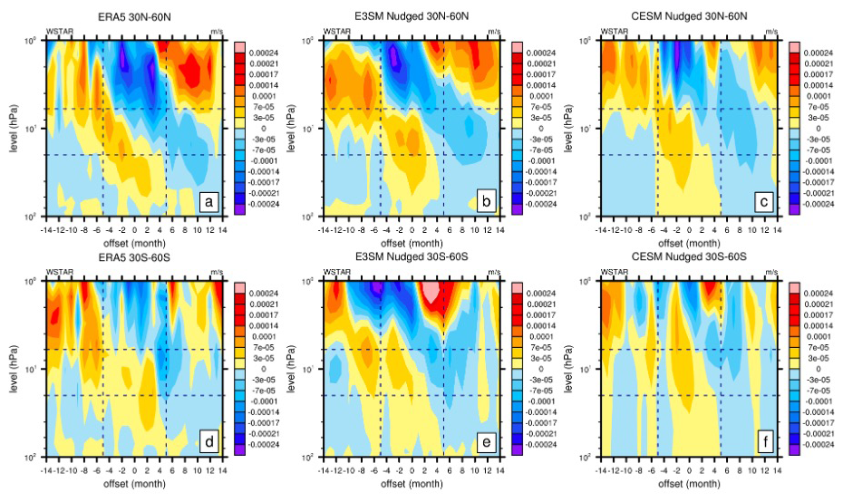
Figure 6 As in Fig. 4 but for the extratropical (30–60° N, 30–60° S) ${\underset{\mathrm{¯}}{w}}^{\ast }$ anomaly (m s⁻¹) as a function of QBO for (a, d) ERA5, (b, e) E3SMv2 nudged, and (c, f) CESM2 nudged for 1979–2020.

To sum up, nudging creates a more realistic QBO signal in both E3SMv2 and CESM2, especially in the tropical region. Outside of the nudging region, the spillover effect of the nudged QBO is seen mostly in temperature and ${\underset{\mathrm{¯}}{w}}^{\ast }$ but less so in the noisier zonal wind.

3.2 Impact of QBO on global TCO

In this section, we examine the impact of QBO on ozone using TCO reanalysis (MSRv2) and E3SMv2 model simulations. The TCO composites from the nudged E3SMv2 simulation are compared in Fig. 7. It is shown that the anomalous MSRv2 TCO exhibits a significant shift of tripole pattern from QBOe to QBOw (Fig. 7a). MSRv2 exhibits a tripole pattern of anomalously low TCO in the tropics and high TCO in the extratropics during QBOe, which gradually changes to an anomalously high and low tripole pattern in the tropics and extratropics during QBOw, respectively. The magnitude of the negative pattern in QBOe (5 DU) is lower than that of the positive pattern (12 DU) in QBOw in the tropics, indicating an asymmetric phase response of TCO to QBO in the tropics. The nudged E3SMv2 simulation is similar to MSRv2 in that it captures most of the tripole patterns in both phases with similar amplitudes (Fig. 7b), indicating that the impact of nudged QBO on TCO is close to what is observed. It is shown that the internally generated QBO variability in the E3SMv2 natural simulations (Fig. S5a) only partly reproduces the patterns of MSRv2, with weaker amplitude (nearly 8 times weaker). Since the response of column ozone is mainly driven by the wind in the lower stratosphere, this discrepancy likely indicates that the internally generated QBO is too weak there. This, along with the good result in the nudging run (Fig. 7b), indicates that nudging the tropical zonal wind contributes to the modulation and enhancement of this QBO-driven TCO variability in E3SMv2.

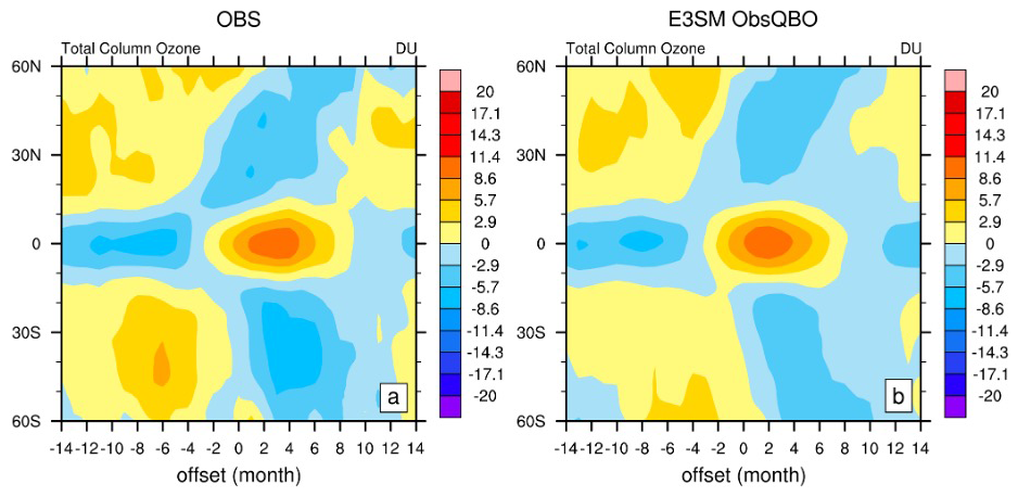
Figure 7 As in Fig. 4 but for a time–latitude map of total column ozone (TCO) anomaly composites (in Dobson, relative to the 1979–2020 mean) as a function of the QBO phase (determined by the NLPCA QBO index) for (a) OBS (Multi-Sensor Reanalysis version 2) and the (b) nudged E3SMv2 simulation for 1979–2020.

Overall, the nudged E3SMv2 simulations show QBO-driven TCO variability in accordance with observations, which is also partly present in E3SMv2 natural simulations and enhanced by QBO nudging.

3.3 Impact of QBO on tropical and extratropical stratospheric ozone

In this section, we analyze the impact of QBO on tropical (15° S–15° N) and extratropical (30–60° S, 30–60° N) stratospheric ozone concentrations. The composites of the ozone vertical profile (1–100 hPa) from nudged E3SMv2 and E3SMv2 Linoz v3 simulations are compared with the CMZM satellite data (Fig. 8).

Figure 8 As in Fig. 4 but for the tropical (15° S–15° N) ozone concentration anomaly (mol mol⁻¹) as a function of the QBO phase for (a) observations (Concentration Monthly Zonal Mean), (b) the nudged E3SMv2 simulation, and (c) the nudged E3SMv2 Linoz v3 simulation for 1979–2020.

In the tropics, it is shown that the ozone observed by the CMZM satellite exhibits a double-peak vertical structure with large ozone variations between 1–20 hPa and 20–100 hPa (Fig. 8a). Both peaks shift in a negative–positive–negative sequence from QBOe to QBOw, and the amplitude of the upper peak is smaller than that of the lower peak (Fig. 8a). The nudged E3SMv2 simulation captures most of the double-peak structure (Fig. 8b) with minor exceptions – the anomalously high ozone in CMZM from month −14 to month −8 around 10 hPa and the anomalously low ozone around 10 hPa from month −2 to month 2 are missed. Studies have shown NO_y variations as the primary drivers of ozone QBO changes around this range (Chipperfield et al., 1994; Tian et al., 2006). Since the nudged E3SMv2 simulation uses Linoz v2, where the chemical species such as CH₄ and NO_y remain constant, the deficiency may be due to uncertainty in these chemical species. To test this assumption, we also compared the nudged E3SMv2 Linoz v3 simulation (with chemistry of NO_y–N₂O–CH₄–H₂O included) with CMZM (Fig. 8c). It is shown that the nudged E3SMv2 Linoz v3 simulation captures both missing ozone fluctuations between 6 and 10 hPa in the nudged E3SMv2 simulation, indicating that this missing chemistry may be responsible for this deficiency. The E3SMv2 natural simulations, on the other hand, show similar double-peaked patterns but with a smaller amplitude (3 times weaker) and shorter period (Fig. S5b). This may be because the period of internally generated QBO in E3SMv2 is ∼21 years (Golaz et al., 2022). Overall, the nudged E3SMv2 simulation modifies the period and enhances the QBO response in tropical ozone, showing a pattern that is mostly consistent with the CMZM – weaker above 20 hPa and stronger below 20 hPa.

This analysis is extended to the nudged E3SMv2 simulations in the extratropical region in both hemispheres (30–60° N, 30–60° S). Since the nudging is imposed only in the tropical regions, we can further examine the impact of nudged QBO in the extratropics where it is free running. Figure 9 shows the pressure–time cross-section of the extratropical (30–60° N, 30–60° S) ozone concentration as a function of the QBO phase for CMZM satellite ozone, the nudged E3SMv2 simulation, and the nudged E3SMv2 Linoz v3 simulation. Unlike that of the tropics, the extratropical ozone for CMZM is noisier, despite an overall in-phase shift with QBO (Fig. 9a and d). The exception is in the NH, where QBOw exhibits an extra phase shift to positive (Fig. 9a). It is shown that nudged E3SMv2 simulations follow a similar positive–negative ozone phase shift in both hemispheres (Fig. 9b and e) without the noisy phase shift in the NH. In terms of the amplitude, QBOw is similar for both hemispheres but weaker than CMZM in QBOe. The ozone change in the nudged E3SMv2 Linoz v3 simulation tends to be similar to that in the nudged E3SMv2 simulation, except that the amplitude in QBOw is stronger (Fig. 9c and f). Overall, the nudged E3SMv2 and E3SMv2 Linoz v3 simulations partly capture the in-phase shift with QBO in extratropical ozone in both hemispheres, despite the amplitude difference.

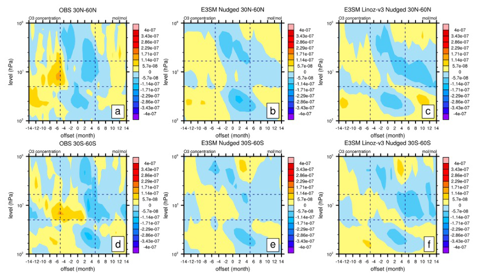
Figure 9 As in Fig. 4 but for the extratropical (30–60° N, 30–60° S) ozone concentration anomaly (mol mol⁻¹) as a function of the QBO phase for (a, d) OBS (CMZM), (b, e) E3SMv2, and (c, f) CESM2 for 1979–2020. The nudged E3SMv2 Linoz v3 simulation is produced using E3SMv2 nudged, with stratospheric chemistry replaced with Linoz v3.

3.4 Separating the chemistry and transport impacts of QBO on ozone using steady-state ozone

In this section, we utilize the SSO (Eqs. 2 and 3; see Sect. 2.5 for details) introduced in Sect. 2.5 to separate the chemistry and transport impacts of QBO on ozone. As a coupled system, the QBO chemical and transport impacts on ozone are intertwined, making it difficult to determine which QBO impact is more important for the ozone differences between models and observations or among different models. Here we try to quantitatively separate these two terms with this new diagnostic tool, recognizing their timescale differences. We first derive the Linoz v2 SSO (Eq. 2) for nudged E3SMv2 and CESM2 simulations (Fig. 10). Although ozone is prescribed in CESM2, the SSO for CESM2 shown here is the temperature–ozone impact due to the CESM2 temperature profiles. To further analyze the impact of temperature and different chemistry species (NO_y, N₂O, H₂O, CH₄) in ozone simulations, the SSO using temperature only (Eq. 2) and using temperature and chemistry species (Eq. 3) is derived for E3SMv2 Linoz v3 nudged (Fig. 11).

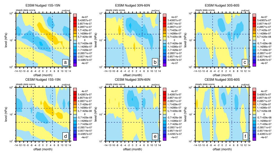
Figure 10 As in Fig. 4 but for the tropical (15° S–15° N) and extratropical (30–60° N, 30–60° S) steady-state ozone anomaly (mol mol⁻¹) as a function of the QBO phase for (a) E3SMv2 and (b) CESM2 for 1979–2020.

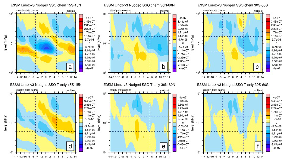
Figure 11 As in Fig. 4 but for the tropical (15° S–15° N) and extratropical (30–60° N, 30–60° S) steady-state ozone anomaly (mol mol⁻¹) as a function of QBO for the nudged E3SMv2 Linoz v3 simulation using (a–c) Linoz v3 chemistry (NO_y–N₂O–CH₄–H₂O) and (d–f) temperature only for 1979–2020.

In the tropics (15° S–15° N), the Linoz v2 SSO from E3SMv2 and CESM2 nudged exhibits an apparent negative–positive–negative pattern above 20 hPa (Fig. 10a and d). This pattern corresponds to the temperature patterns above 20 hPa shown in the previous section (Fig. 4b and c). This pattern in E3SMv2 is similar to that of the E3SMv2 ozone pattern above 20 hPa (Fig. 8b), indicating a temperature impact mostly above 20 hPa. Below 20 hPa, the prognostic ozone in E3SMv2 corresponds to the alternating ${\underset{\mathrm{¯}}{w}}^{\ast }$ shift patterns (Fig. 4e). The residual meridional circulation shows a weaker magnitude below 20 hPa and is thus less likely to play a major role in ozone change (Fig. S6). This and the lack of response in SSO indicate that the prognostic ozone below 20 hPa in E3SMv2 is transport driven. Similar to that of the analysis in the tropics, the temperature impact in the extratropics (30–60° N, 30–60° S) is stronger above 20 hPa for both nudged E3SMv2 (Fig. 10b and c) and nudged CESM2 (Fig. 10e and f) simulations. The difference is that temperature in the SH (30–60° S) is overall noisier than that in the Northern Hemisphere (30–60° N). This noisier SH SSO above 20 hPa in the nudged simulations corresponds to the noisier temperature for the two models (Fig. 5c and f), which may be largely affected by a stronger and noisier southern polar vortex (Fig. S7), as also documented by other studies (Ribera et al., 2004). The intrusion of the polar vortex via events like sudden stratospheric warming (Butler et al., 2017) may have an impact on the QBO–ozone relationship in the extratropics. Below 20 hPa, the nudged E3SMv2 ozone corresponds to ${\underset{\mathrm{¯}}{w}}^{\ast }$ (Fig. 10b and e), indicating it is transport driven. Overall, with the application of Linoz v2 on the nudged E3SMv2 simulation, we can partly separate the temperature-driven and transport-driven QBO–ozone around the boundary of 20 hPa in both the tropics and the extratropics. The limitation of this application lies in the uncertainty in the exclusion of chemistry transport, such as NO_y, in the simulations.

To test the sensitivity of the results to the chemistry variations, we further applied Linoz v2 SSO (Eq. 2, temperature only) and Linoz v3 SSO (Eq. 3, temperature and chemistry) to the nudged E3SMv2 Linoz v3 simulation (Fig. 11). It is shown that the SSO including temperature and chemistry variation shows better agreement with MSRv2 ozone (Figs. 8a and 9a and d) compared to the SSO including temperature only, especially in both the tropics (Fig. 11a and d) and the extratropics (Fig. 11c–f). This better agreement is especially apparent between 6 and 20 hPa and is in good agreement with the NO_y change (Fig. 12), indicating the impact of chemistry variation within this height. To further examine the variable responsible for the change, we also conducted the single-species sensitivity test (not shown). It is shown that including temperature and NO_y variation can reproduce the patterns in Fig. 11a–c. This indicates that the NO_y variation is an important driver around 6 to 20 hPa in QBO–ozone, in accordance with previous studies (Chipperfield et al., 1994; Tian et al., 2006).

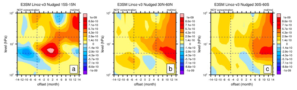
Figure 12 As in Fig. 4 but for the tropical (15° S–15° N) and extratropical (30–60° N, 30–60° S) NO_y anomaly (mol mol⁻¹) as a function of QBO for (a–c) E3SMv2 Linoz v3 between 1979–2020.

The results here indicate demarcations of QBO-induced ozone at 6 and 20 hPa. These demarcations of the QBO-induced ozone at 6 and 20 hPa may be due to the separation of ozone lifetime below and above 20 hPa (Reed, 1964) and NO_y variation (Chipperfield et al., 1994; Tian et al., 2006). The ozone lifetime is relatively long compared with the dynamical process below 20 hPa, while it is shortened considerably above 20 hPa. Temperature affects ozone above 20 hPa (especially above 6 hPa) through ozone destruction – warmer anomalies accelerate ozone destruction, leading to a correspondent ozone decrease (Wang et al., 2022); vice versa, the transport effect of QBO-related wind modulates temperature through thermal wind balance enhancing/lessening the upward motion in the tropics (Plumb and Bell, 1982; Baldwin et al., 2001; Ribera et al., 2004; Punge et al., 2009). In the extratropics, the process is similar, except that is controlled by the downward branch of QBO-induced circulation that is in 180° phase reversal with the tropics (Baldwin et al., 2001). This explains the apparent separation of transport- and chemistry-driven ozone changes above and below 20 hPa. Between 6 and 20 hPa, QBO modulation of NO_y variation, in addition to the temperature impact, is shown to be an important contributor to the QBO–ozone cycle (Chipperfield et al., 1994). This explains the better reproduction of SSO above 20 hPa when including NO_y variation. Ozone transport, on the other hand, plays a relatively weaker role above 20 hPa. Overall, the demarcations of QBO-induced ozone shown here can generally be explained by photochemical processes above 6 hPa, NO_y variation between 6 and 20 hPa, and circulation change in vertical advection below 20 hPa. It is also worth mentioning that the nudged CESM2 also produces a similar temperature and ${\underset{\mathrm{¯}}{w}}^{\ast }$. This indicates that nudged CESM2 may produce similar prognostic ozone if Linoz were to be implemented as an interactive ozone module.

3.5 Model performance in simulating QBO impact

In this section, we examine the overall performance of E3SMv2 and CESM2 QBOi simulations in simulating the QBO–ozone relationship. We evaluate the pattern correlation and standard deviation of the area-weighted TCO pattern (60° S–60° N), vertically weighted ozone concentration (15° S–15° N, 30–60° N, 30–60° S), zonal wind (15° S–15° N, 30–60° N, 30–60° S), temperature (15° S–15° N, 30–60° N, 30–60° S), and ${\underset{\mathrm{¯}}{w}}^{\ast }$ (15° S–15° N, 30–60° N, 30–60° S). For ozone, only E3SMv2 results are shown since CESM2 has fixed ozone. The results are summarized in a Taylor diagram shown in Fig. 13. The observed pattern is plotted at the (1,0) reference point.

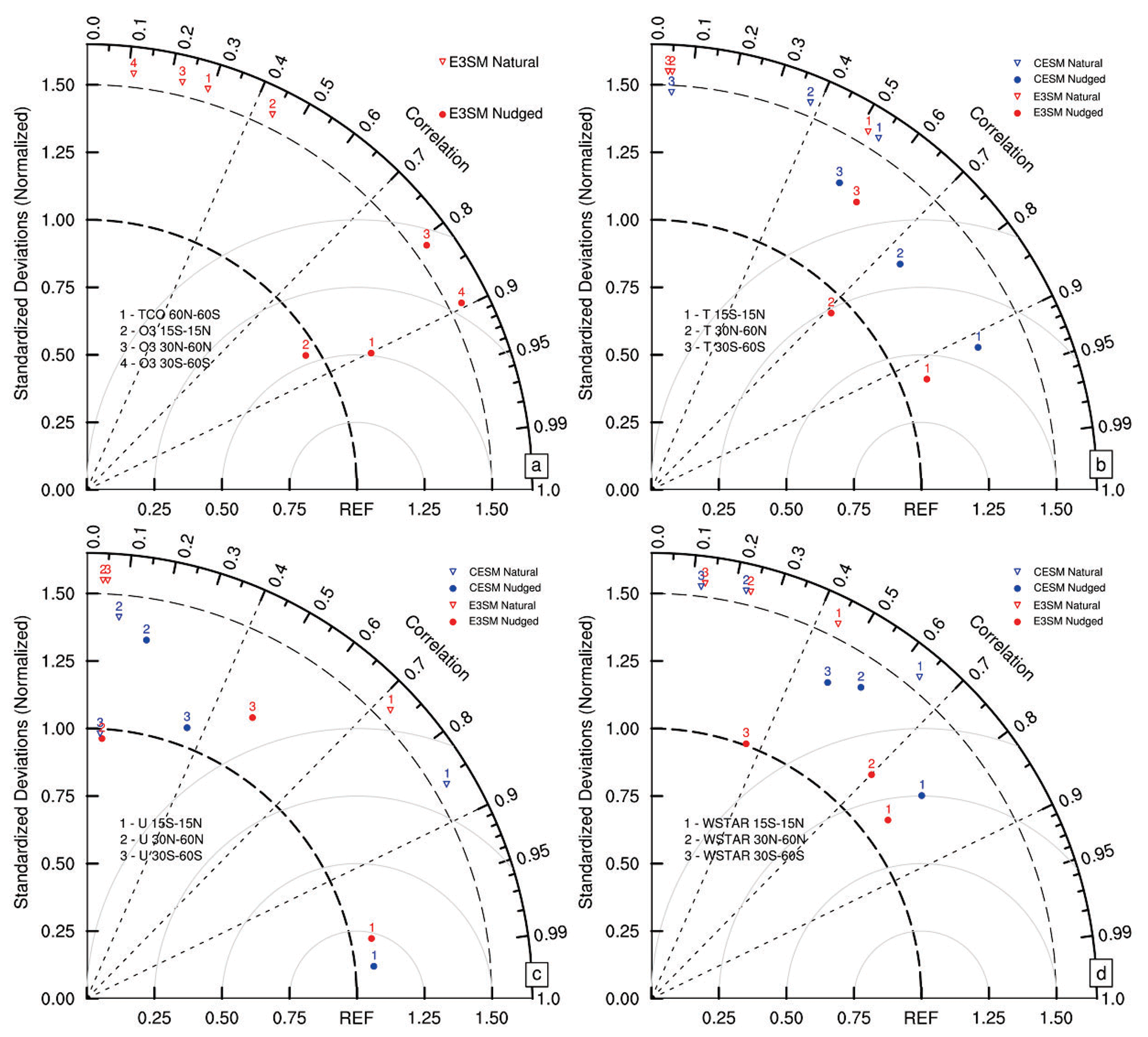
Figure 13 Taylor diagram of the E3SMv2 and CESM2 simulations for various datasets for 1979–2020. (a) The area-weighted total column ozone (60° S–60° N; DU) and pressure–time cross-sections of ozone concentration (15° S–15° N, 30–60° N, 30–60° S; mol mol⁻¹) anomalies with OBS (MSR and CMZM). (b) The area-weighted pressure–time cross-sections of temperature (15° S–15° N, 30–60° N, 30–60° S; K) anomalies with ERA5. (c) The area-weighted pressure–time cross-sections of zonal wind (15° S–15° N, 30–60° N, 30–60° S; m s⁻¹) anomalies with ERA5. For pattern correlations, the cross-sections are weighted by pressure layer thickness. On all Taylor diagrams, the model standard deviations are normalized by dividing the standard deviations of the reference.

In terms of ozone (Fig. 13a), there are remarkable differences between the simulations. Overall, the nudged E3SMSv2 simulations perform the best, with the pattern correlation of all four variables over 0.8, while that of other simulations are below 0.5. This indicates nudging realistic QBO variability may increase the model performance in simulating ozone. In the extratropics, the nudged E3SMv2 simulation has good pattern correlations, but the amplitude is off by over 1.5. The results for temperature, zonal wind, and ${\underset{\mathrm{¯}}{w}}^{\ast }$ are similar with ozone in the tropics (Fig. 13b–d). What is different is in the extratropics – both nudged E3SMv2 and nudged CESM2 temperature, zonal wind, and ${\underset{\mathrm{¯}}{w}}^{\ast }$ show better performance in the NH extratropics than in the SH extratropics. This may be due to stronger polar vortices in SH and NH that disturb the QBO signal (Ribera et al., 2004). Another difference is in the natural simulations – the tropical temperature (15° S–15° N) and zonal wind signals exhibit reasonable correlations of over 0.7 in zonal wind and over 0.5 in temperature. This indicates a discernable internally generated QBO signal in E3SMv2 and CESM2, although it is weaker and does not extend to the extratropics.

4 Discussion and conclusion

4.1 Discussion

There are some interesting issues worth discussing in this section. First, the use of the SSO provides a useful tool to determine the dynamical and chemical impact of the QBO on ozone. The Linoz v2 SSO metric can be applied to all models with the minimum need of a temperature profile only. One caveat of this approach is that the Linoz v2 SSO neglects the potential impact of cross-over chemical species such as NO_y, as this has been shown to be an important driver of QBO–ozone change between 6 and 20 hPa in SSO. Thus, it is recommended to include at least the NO_y output by the CCMs in SSO calculation (Eq. 3) for a more precise diagnostic between this height range. The QUasi-Biennial oscillation and Ozone Chemistry interactions in the Atmosphere (QUOCA) proposed a new joint QBOi–CCMI project to improve our understanding of the QBO–ozone feedback in present-day and future climates. The tools shown here may be useful to determine the uncertainty in the QBO–ozone relationship among different model simulations in this project.

Another noteworthy issue is the nudging employed in the current study. Nudging has been adopted by models from different climate centers in the QBOi project to ensure the realistic simulation of QBO by constraining the tropical climate. The different strategies of nudging in these models and their effects on the QBO climate thus need to be analyzed with care. Our study showed that the nudging overall constrains both E3SMv2 and CESM2 towards a realistic representation of QBO-associated temperature and a residual circulation field outside of the nudged regions (15° S–15° N; tropics). However, differences in the nudging strategies can play a role in the detailed features of the zonal wind and temperature simulated by the two models. For example, the extratropical zonal wind and temperature in CESM2 showed more scattered features than those in E3SMv2 in our simulations. This may be partly because the full-field nudging in E3SMv2 nudges all zonal wavenumbers. This may pose a stronger constraint on the field than the zonal mean nudging in CESM2, which may nudge a narrower spectrum of zonal wavenumbers.

Thirdly, our study shows the importance of including NO_y–N₂O–CH₄–H₂O chemistry in the linearized ozone representation of a climate model. We show that the E3SMv2 Linoz v2 simulation with linearized ozone may underestimate the QBO–ozone amplitude above 10 hPa, as also documented in Meraner et al. (2020). The E3SMv2 Linoz v3 simulation with NO_y–N₂O–CH₄–H₂O chemistry, on the other hand, improves this QBO–ozone magnitude, especially between 6 and 10 hPa. Meraner et al. (2020) demonstrated the usefulness of linearized ozone in representing ozone due to negligible computational cost, despite its deficiency in simulating QBO–ozone magnitude. The inclusion of NO_y–N₂O–CH₄–H₂O chemistry may contribute to alleviating this issue.

Last, the impact of ozone feedback on the climate in this study requires further attention. The two models compared here show overall similar QBO signals over the nudging runs, despite having two different ozone modules – one interactive and the other non-interactive. One may question what the results would be with the same modules under nudging. The sensitivity test of the nudged E3SMv2 fixed-ozone simulation shows that with fixed ozone, the temperature patterns are still retained, although with an amplified magnitude in both the tropics and the extratropics (Fig. S8). This indicates a strong nudging impact and an overall damping effect of interactive ozone in E3SMv2.

4.2 Conclusion

In this study, we utilize the SSO on nudged climate model simulations to separate the chemical and transport responses of the QBO ozone impact. We derive a new QBO phase index using the NLPCA method and utilize this index to form QBO cycle composites to analyze QBO–ozone relationships in observations and simulations. By analyzing the simulations from two QBOi participant models (E3SMv2 and CESM2), we found that the nudged simulations can produce a reasonable QBO impact in the tropics and create a spillover impact on extratropical fields, like temperature and residual circulation. The nudged E3SMv2 simulation captures the tripole composite pattern in the observed TCO. Nudging was also shown to improve the double-peaked vertical structure in observed ozone data between 1–20 and 20–100 hPa over the tropics. In the extratropics outside of the nudging region, the nudged E3SMv2 simulated ozone tends to generally be in phase with the observations but with a magnitude difference, indicating the spillover impact of the nudged QBO signal.

Utilizing the SSO metric, we separated the chemical and transport responses of ozone in E3SMv2 nudged to QBO. It is shown that these impacts have rather clear demarcations on both the tropical and the extratropical ozone response at 6 and 20 hPa – the chemistry impact corresponding to QBO-related temperature changes dominates the response above 6 hPa, linked to photochemical processes, and between 6 and 20 hPa, linked to NO_y variation. The transport impact associated with QBO-related vertical advection dominates the response below 20 hPa. The results here are important for diagnosing model–model and model–observation differences in the QBO with free-running climate simulations, allowing us to separate chemical effects from circulation effects.

Stratospheric ozone is essential not only for protecting life on Earth but also for impacting the climate. More and more studies report the important role of ozone variations in modifying stratospheric circulation and therefore influencing the surface climate (e.g., Xie et al., 2020). Since the QBO has relatively high predictability, considering its impacts on stratospheric ozone and subsequent atmospheric circulations may help improve the predictions of surface weather and climate (e.g., Li et al., 2023).

Despite the above studies, however, there are still caveats. The current study makes use of only one model in QBOi that has an interactive ozone feature. More models may be used in the future to examine the QBO–ozone relationship. These are to be assessed in future studies.