the Creative Commons Attribution 4.0 License.
the Creative Commons Attribution 4.0 License.
To what extent is the description of streets important in estimating local air quality: a case study over Paris
Alexis Squarcioni
Yelva Roustan
Myrto Valari
Youngseob Kim
Karine Sartelet
Lya Lugon
Fabrice Dugay
Robin Voitot
Modeling atmospheric composition at street level is challenging because pollutant concentrations within street canyons depend on both local emissions and the transport of polluted air masses from remote areas. Therefore, regional-scale modeling and local applications must be combined to provide accurate simulations of the atmospheric composition at street locations. In our study, we compare two strategies: (i) a subgrid-scale approach embedded in the chemistry–transport model (denoted Subgrid) and (ii) the street-network model MUNICH (Model of Urban Network of Intersecting Canyons and Highways). In both cases, the regional-scale chemistry–transport model CHIMERE provides the urban background concentrations, and the meteorological model Weather Research and Forecasting (WRF), coupled with CHIMERE, is used to provide meteorological fields. Simulation results for NOx, NO2, and PM2.5 concentrations over the city of Paris from both modeling approaches are compared with in situ measurements from traffic air quality stations. At stations located in downtown areas, with low traffic emissions, the street-network model MUNICH exhibits superior performance compared to the Subgrid approach for NOx concentrations, while comparable results are obtained for NO2. However, significant discrepancies between the two methods are observed for all analyzed pollutants at stations heavily influenced by road traffic. These stations are typically located near highways, where the difference between the two approaches can reach 58 %. The ability of the Subgrid approach to estimate accurate emission data is limited, leading to potential underestimation or overestimation of gas and fine-particle concentrations based on the emission heterogeneity it handles. The performance of MUNICH appears to be highly sensitive to the friction velocity, a parameter influenced by the anthropogenic heat flux used in the WRF model. Street dimensions do contribute to the performance disparities observed between the two approaches, yet emissions remain the predominant factor.
- Article
(6103 KB) - Full-text XML
- BibTeX
- EndNote
Numerous research studies assessed the consequences of atmospheric pollutants in terms of harmful health effects and premature deaths (WHO, 2013, 2021), as well as the impacts on ecosystems and biodiversity (Marcoa et al., 2019; WGE, 2016). A vast majority of the world's cities suffer from significant atmospheric pollution problems (Sicard et al., 2023), representing a prominent threat to human health and the global environment. A significant part of the European population is exposed to concentrations above the limit or target values (EEA, 2023). Exposure to a high concentration of particulate matter is one of the most harmful effects of atmospheric pollution (Lelieveld et al., 2015).
Results from these investigations motivate progress in air quality modeling, in order to more precisely estimate pollutant concentrations and dispersion at decisive (i.e., local) spatial scales (Lugon et al., 2022). Models are valuable to understand and support the control of the evolution of air quality inside cities.
Several approaches exist to assess air pollutant concentrations at local scales in urban built-up environments. The scientific and practical relevance of their use depends on the objectives and issues to be addressed.
As explained in Kiesewetter et al. (2013), local estimations of gas or particulate matter concentrations are obtainable from regional modeling by the implementation of downscaling coefficients to determine urban and roadside increments. Despite variations on the mathematical implementation, the general methodology of the local increments has been used (Lenschow et al., 2001), and it is based on the estimation of the impact of the city and of the local traffic, which is added to the regional background.
However, some research studies (Longley et al., 2014; Thunis, 2017) highlight the dependence of these local increments on crucial parameters such as wind direction, wind speed, and station location. The implicit empirical adjustment inherent in this type of approach, based on statistical processing of observation data, makes them difficult to transfer from one city to another. Alternative statistical methods, introducing more explicitly site-specific geographical information, exist and can be efficient in terms of computation time or quantity of necessary data. For instance, land-use regression (LUR) models (Azmi et al., 2023; Dons et al., 2013) based on regression methods to solve the spatial variability of concentrations through a set of spatialized information (traffic, population density, etc.) are often used in dense urban areas. However, as reported in Hatzopoulou et al. (2017), LUR models are only robust in regions where dense measured data are available. The quantity of necessary data for optimum results could change from one city to another, depending on the urban density.
In the range of methods based on first principles (i.e., resolution of conservation equations), the computational fluid dynamics (CFD) models provide very fine descriptions of air pollution concentrations at the street scale. This modeling technique handles extremely intricate wall shapes and other boundary conditions through the use of flexible fine-scale grids. Additionally, CFD models incorporate advanced approaches to take into account turbulence, making it well-suited for applications involving small-scale dispersion of pollutants. This type of model is widely used to analyze specific urban configurations on a neighborhood scale (Sabatino et al., 2013; Zhang et al., 2020; Pantusheva et al., 2022; Lin et al., 2023), but the computing times required to simulate a large urban area over periods of time on the order of a year are currently unattainable. With this type of temporal and spatial constraint, compatible with regulatory objectives (e.g., compliance with a threshold for an annual average concentration) or a health impact study, methods with lower computational burdens are currently mandatory. Deterministic models, relying on simplified representations of street topology and atmospheric flow in streets, have been developed for years. In this category, we can mention the Operational Street Pollution Model (OSPM; Berkowicz, 2000) and its evolution in the Atmospheric Dispersion Modeling System (ADMS-urban; Stocker et al., 2012). These models combine a Gaussian plume to estimate the direct contributions of traffic emissions and a box model to calculate the background concentration in the recirculation zone attributable to the surrounding buildings. Additionally, the street-network model SIRANE (Soulhac et al., 2011) has also been developed to represent pollutant dispersion within a dense urban canopy. This model assumes that pollutant concentrations are uniform along each street section but explicitly represents the pollutant transfer via street intersections. The dispersion above roof level is handled by a Gaussian plume model. The Model of Urban Network of Intersecting Canyons and Highways (MUNICH; Kim et al., 2018) also uses an explicit representation of street sections, but the dispersion above roof level can be treated with an Eulerian approach by coupling to a chemistry–transport model.
The aforementioned approaches use simplified chemical mechanisms to represent the formation and evolution of atmospheric pollutants. The use of a Gaussian plume model indeed implies a stationary assumption which is not compatible with the modeling of complex physicochemical transformations. This may be a source of substantial uncertainties in air pollution simulations. Particulate matter can be emitted directly but can also appear after a series of complex chemical formation processes (Fuzzi et al., 2015). Thus, more comprehensive chemical modules must be applied for a consistent representation of the gas-phase chemistry and the secondary formation of aerosols (condensation/evaporation, coagulation, nucleation). The coupling of models from different scales is an efficient way to represent local pollutant concentrations, especially near roadside sites for NOx, NO2, and O3 (Hooyberghs et al., 2022; Hamer et al., 2020; Lugon et al., 2020; Benavides et al., 2019; Karl et al., 2019; Hood et al., 2018; Berchet et al., 2017; Beevers et al., 2012). To be able to represent the formation of secondary gas and particles at local scales, the MUNICH street-network model was coupled to the “SSH-aerosol” chemistry and aerosol dynamic model (Sartelet et al., 2020) to provide a detailed evolution of primary and secondary aerosols (Lugon et al., 2021; Kim et al., 2022a).
The purpose of this paper is to compare two different downscaling methods, both using as starting point regional-scale simulations with CHIMERE (Menut et al., 2021) driven by meteorological fields derived from the Weather Research and Forecasting (WRF) model (Skamarock et al., 2005; Mailler et al., 2017; Briant et al., 2017; Tuccella et al., 2019) at 1 km × 1 km resolution. The first method consists of the subgrid-scale model embedded in CHIMERE (denoted Subgrid) (Valari and Menut, 2010), which splits the grid-averaged pollutant concentration into a set of source-specific components based on land-use fractions to represent the subgrid-scale area. The other approach is to use the MUNICH model, which requires explicit information on the street sections of the road network, namely, the length, the mean width, and the mean height of surrounding buildings. Therefore, we are interested in identifying the conditions under which these two approaches provide similar or diverging simulation results. The simulations performed to compare the methods are conducted over greater Paris, and model results are compared against observations at several traffic-monitoring sites with different characteristics: inside street canyons, at roundabouts, or at open roads not bounded by buildings. The street-network model MUNICH and the Subgrid method of CHIMERE are briefly described in Sect. 2. The model setup and input databases for the simulations, with an emphasis on the use of an urban canopy model in WRF, are described in Sect. 3; monitoring data are detailed in Sect. 3.3. The results of the study are presented in Sect. 4. Section 5 is the conclusion of the comparative study between the two methods.
Only the main concepts of the two modeling approaches are recalled here. The details of the implementations of the models are provided in Valari and Menut (2010) for the Subgrid method of CHIMERE and in Kim et al. (2018, 2022a) and Lugon et al. (2020) for the MUNICH model.
2.1 The CHIMERE subgrid-scale method
CHIMERE is a 3D Eulerian model that numerically solves a set of equations which represents the transport and chemical transformation of several chemical species in the atmosphere. It is a mesoscale model with a horizontal resolution that ranges from 1 to 100 km, corresponding to study areas that may cover an urban agglomeration to an entire hemisphere.
The SSH-aerosol model, named after the three models it incorporates – SCRAM (Zhu et al., 2015), SOAP (Couvidat and Sartelet, 2015), and H2O (Couvidat et al., 2012) – has been recently integrated into CHIMERE. This model provides a detailed representation of the formation and dynamic evolution of atmospheric aerosols (Maison et al., 2024; Wang et al., 2024). Typically, CHIMERE, as all 3D Eulerian models, assumes that surface emissions are homogeneous over each model grid cell. However, the subgrid-scale model introduced in Valari and Menut (2010) has been implemented in CHIMERE v2020 (Menut et al., 2021) and accounts for the heterogeneity of surface emissions due to the action of different activity sectors within the same model grid cell. The model transfers this emission heterogeneity to concentration variability (Valari and Menut, 2010). In practice, the model uses two pieces of information: emissions from different activity sectors and an area fraction for each model grid cell occupied by each sector taken into account. In this study, we separate emissions into two sectors: those from traffic and those from all other sectors. Following the subgrid-scale scheme implemented here, high emissions from roads are condensed over relatively narrow areas (roads), leading to intensified emissions from the traffic sector compared to the grid-averaged emission that would have been diluted to the entire grid-cell volume.
Following this approach, the set of transport equations is solved separately for each considered sector. Equation (1) gives the temporal evolution of the concentration for a given species for each different subgrid surface:
where ci is the concentration computed for the ith sector, and is the grid-averaged concentration in the cell. The terms from left to right represent the advection by the mean wind U, the turbulent mixing parameterized by a gradient diffusion hypothesis with K being a matrix of turbulent diffusion coefficient, the emissions from the ith sector (Ei), the source and loss terms associated with chemical transformations (Ri), and the deposition inside the ith subgrid volume (Li). Finally, the last term accounts for a mixing of concentrations calculated for the different subgrid volumes. The rate of the mixing is controlled by the term Tmix, which is the ratio between a characteristic length (different in every grid cell for each emitting surface) and the mean local wind speed.
The advantage of this approach is that the full chemical mechanism operates over each subgrid-scale volume, i.e., for each sector specifically considered, leading to subgrid-scale concentrations for all model species. The limitation of the approach is that it does not explicitly take into account (i) the effect of the buildings on the flow of pollutants and (ii) the emission over each road. As a result, the different street sections within a given cell are not treated separately but rather as an average road configuration inside the grid cell.
2.2 The street-network model MUNICH
MUNICH is a street-network model designed for simulating pollutant concentrations at a local scale. To achieve this, the model needs input data such as background pollutant concentrations, meteorological information, and emissions to accurately simulate concentrations within the street network. The street network is composed of two types of elements: the street segments and the street intersections. Pollutant concentrations are only resolved for street segments and are assumed to be homogeneous inside each one of them. The integration of the mass conservation equation (Eq. 2) provides the temporal evolution of the concentration for a given species for each different street segment treated as a box model:
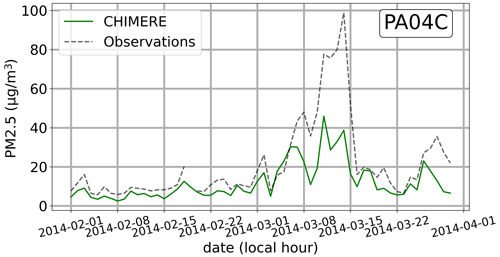
where ci is the concentration (in µg m−3) computed for the ith street segment to which are assigned a length (L), a mean width (W), and a mean buildings' height (H) assumed to be the same on both sides of the road. These three characteristics are in meters. Vi is the volume (in m−3) of this rectangular cuboid street. The mean wind in the street is parallel to the street axis. Qi,inflow and Qi,outflow (in µg s−1) are, respectively, the mass flux entering the street via the upwind intersection and the mass flux leaving the street via the downwind intersection (both in µg s−1). A double mass balance, for air and pollutants, determined for each intersection, allows us to constrain, relying on the concentrations in the others streets connected and the boundary conditions cbg, the advective entering flux. Qi,vert is the vertical turbulent flux (in µg s−1) between the background (here corresponding to concentrations simulated by CHIMERE) and the street. In the framework of the one-way coupling strategy applied in this work, as in many previous studies (e.g., Sarica et al., 2023; Wang et al., 2022), the background concentrations are not modified by MUNICH. These simulated background concentrations are evaluated against observations in Appendix D. This comparison shows that CHIMERE is able to provide boundary conditions for MUNICH that are representative of the background concentrations observed. Ei represents the emissions from traffic, Ri combines the source and loss terms associated with chemical transformations, and Li is the deposition inside the ith street segment (all three in µg m−3 s−1). As with the CHIMERE subgrid-scale model, the full chemical mechanism is applied to each street, leading to street-scale concentrations for all the species in the model.
Below, we recall a few more specific aspects of the MUNICH model parameterizations to highlight (i) the influence of the aspect ratio of the street (the ratio of the mean height to the mean width) and (ii) the influence of the friction velocity and the atmospheric stability.
The vertical turbulent flux is computed using the boundary condition cbg as follows:
where cbg is the background concentration (in µg m−3), and represents the aspect ratio of the street. When this parameter, αr, is less than or equal to , the street is classified as a “wide canyon”. For ratios between and , it is categorized as an “intermediate street”, and if the ratio is greater than , the street is designated as a “narrow canyon”. The parameter qv is the vertical transfer coefficient, that corresponds to the following equation:
where σw is the standard deviation of the vertical wind speed, and lm is the mixing length determined using the formulation from Wang (2011). Regarding σw, which depends on the friction velocity u∗ and atmospheric stability, three distinct parameterizations are employed to compute this variable, each corresponding to a different atmospheric state. As proposed for SIRANE in Soulhac et al. (2011) and Salizzoni et al. (2009), MUNICH computes σw following Cambridge Environmental Research Consultants (2001) and Hunt et al. (1988).
The implementation of the different parameterizations available in MUNICH to determine the average wind speed in a street is detailed in Maison et al. (2022). The first step is to compute the wind speed at the mean height of the building, uH. It can be derived in MUNICH from a representative wind speed above the urban canopy or from the friction velocity u∗. This second option and the parameterization of Macdonald et al. (1998) are used in the current work, allowing an estimate of uH based on an average vertical profile at the scale of a neighborhood.
Then, only the component of the wind in the direction of the street is taken into account to reconstruct the wind vertical profile in the street. It has been represented in the current study following the work of Wang (2011, 2014). Finally, the average wind speed in the street is obtained by integrating the chosen wind profile between the soil roughness and the building height.
The subsequent section outlines the input data for regional and local modeling, along with their configuration setup. It includes details about the regional domains utilized, the street network, and their associated emissions, as depicted in Fig. 1.
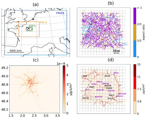
Figure 1(a) The three-level nested simulation domains used to calculate background concentrations (CHIMERE) and meteorological fields (WRF). (b) The street network used for the MUNICH simulations. The color bar represents the road aspect ratio (ratio between the mean height and the mean width of the street); (c) 2-month-averaged NO2 emission flux (February and March 2014) summed across all activity sectors over the CHIMERE IDF1 grid; (d) 2-month-averaged NO2 traffic emission flux (February and March 2014) on the MUNICH street network with the location of the measurement stations (dots) and the CHIMERE-WRF mesh (grid lines). Traffic stations are represented by black dots, and background stations are represented by purple dots.
3.1 Regional scale
Regional-scale concentrations are simulated with the CHIMERE-WRF coupled system (Menut et al., 2021, https://www.lmd.polytechnique.fr/chimere/, last access: 28 October 2024), enriched with the implementation of the SSH-aerosol model (Sartelet et al., 2020, https://sshaerosol.wordpress.com/, last access: 28 October 2024). To obtain pollutant concentrations at 1 km × 1 km resolution, we use a three-level nesting configurations, as shown in Fig. 1a. The largest domain (FRA9) covers France, with a spatial resolution of 9 km × 9 km. The intermediate domain (IDF3) covers part of the north of France, centered around the Île-de-France region with a spatial resolution of 3 km × 3 km. The innermost domain covers the entire Île-de-France region, centered around the city of Paris (IDF1) at a spatial resolution of 1 km × 1 km.
3.1.1 CHIMERE input data
Initial and boundary conditions for the largest CHIMERE domain (FRA9) are taken from the general circulation model LMDz-INCA (Hourdin et al., 2006), with a horizontal resolution of 2.5° × 1.27° and 39 vertical levels. Anthropogenic emissions for the two larger domains are computed from the 2014 EMEP (European Monitoring and Evaluating Program) emission inventory, with a spatial resolution of 0.1° × 0.1°. Anthropogenic emissions for the domain over the Île-de-France region (IDF1) stem from the local, bottom-up inventory of 2014, developed and provided by the Airparif air quality agency of Île-de-France. Biogenic emissions are estimated with MEGAN (Model of Emissions of Gases and Aerosols from Nature; Guenther et al., 2012), embedded in CHIMERE. Meteorological variables are computed with WRF running simultaneously with CHIMERE without activation of feedback from CHIMERE to WRF.
3.1.2 WRF model configuration and input data
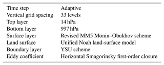
The WRF model configuration used for this study is shown in Table 1. The initial and boundary conditions for the WRF simulations come from the National Centers for Environmental Prediction (NCEP) model and the FNL (Final) dataset (NCEP Weather Service/NOAA/U.S. Department Of Commerce, 2000).
By default, the coupled CHIMERE-WRF model uses the 2004 land-use dataset derived from the Moderate Resolution Imaging Spectroradiometer (MODIS), with a resolution of 1 km. However, for the current study we used a reclassification of the CORINE categories (from CORINE Land Cover data 2018, with a resolution of 250 m) to MODIS-IGBP based on Vogel and Afshari (2020). With three distinct urban categories, this dataset provides a finer spatial representation of the heterogeneous urban area of the Île-de-France region.
This modification is motivated by the use of an urban canopy model, the SLUCM (Single-Layer Urban Canopy Model; Kusaka et al., 2001), applied for this study in the two inner nests, IDF1 and IDF3 (simulations over the largest FRA9 domain run without it). The use of an urban canopy model is required to avoid nonrealistic extremely low values of the friction velocity (u∗), which drives the transfer of mass between the background and the streets in MUNICH (see Eq. 3). Very low values of u∗ lead to concentration peaks in streets with high emissions.
3.1.3 Activation of the urban canopy model
WRF provides different surface layer schemes to compute u∗ and exchange coefficients for heat, moisture, and momentum. Among others, we can cite two surface layer schemes: (i) the MM5 (fifth-generation Pennsylvania State University National Center for Atmospheric Research Mesoscale Model) scheme and (ii) its revised version proposed by Jiménez et al. (2012). In our simulations, we used the revised MM5 scheme (see Table 1), which sets lower limit values for the friction velocity (0.001 m s−1 by Jiménez et al., 2012) than the original MM5 scheme (0.1 m s−1) over land surface, in order to apply a surface layer formulation capable of covering the full range of atmospheric stabilities.
Figure 2 shows u∗ time series at a model grid cell in the urban area with and without an urban canopy model. Without the urban canopy model, extremely low values of u∗ are especially observed during the air pollution episode (first half of March 2014), which is not surprising for a meteorological situation characterized by highly stable conditions (Dupont et al., 2016). However, these low values may not be realistic in urban environments (Liu et al., 2009). Urban canopy models apply urban roughness sublayer corrections to improve Monin–Obukhov similarity theory (Theeuwes et al., 2019) and result in more realistic vertical profiles of wind speed and friction velocity.
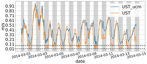
Figure 2Friction velocities simulated by the WRF model during the 2 weeks of the air pollution episode of March 2014 for one cell in Paris. The blue line represents a simulation with the SLUCM, and the orange line represents a simulation without the SLUCM. Nighttime is represented by the gray background. The upper dashed line is the minimum of the blue line, equal to 0.078 m s−1, and the lower dashed line is the minimum of the orange line, which corresponds to 0.01 m s−1.
The WRF model provides different urban canopy models to take into account the effects of urban spaces. Through different geometric and thermal parameters, these models evaluate the surface energy balance and the wind shear in the urban landscapes and provide better representations of the transfer of energy and momentum in cities (Wang et al., 2011). Three urban canopy models are available in WRF: (i) the Single-Layer Urban Canopy Model (SLUCM; Kusaka et al., 2001), (ii) the Building Environment Parameterization (BEP) model (Martilli et al., 2002), and (iii) the Building Energy Model (BEM; Salamanca and Martilli, 2009). The first one is composed of a single layer, whereas the others correspond to multi-layer models. According to Allen et al. (2010), the total anthropogenic heat flux released by a city can be divided into three components: the metabolic, the motorized vehicles, and the building heat emissions. The latter is well modeled by BEP and BEM; however, these models do not offer the possibility to add other sources of anthropogenic heat like the traffic component that cannot be neglected in a large city (Pigeon et al., 2007). Thus, we chose the SLUCM scheme for our simulations, which enables us to increase the anthropogenic sensible and/or latent heat flux in order to represent car traffic heat. Nonetheless, the current study does not consider latent anthropogenic heat flux due to limited literature data on this topic.
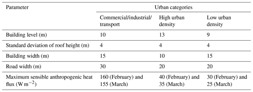
The SLUCM scheme requires maximum values of anthropogenic heat fluxes (Qf) for each considered urban category and a diurnal variation profile to modulate these fluxes over time. The daily profile of this heat flux is assumed to be constant from day to day in the model, and a single maximum is assigned for each urban category. In the case of long simulations (at least several months), the configuration of this urban canopy model must be changed, because the anthropogenic heat flux depends strongly on seasonal temperature variation. For instance, during the summer period, waste heat generated by air conditioning systems strongly impacts urban air temperatures (Salamanca et al., 2015; Tewari et al., 2017). Therefore, two different Qf maximums are settled for February and March 2014 according to Sailor et al. (2015) and Allen et al. (2010). Based on data from Sailor et al. (2015) for Paris, which reported a value of 39.95 W m−2 for the entire city during winter, we opted for a closely aligned value of 40 W m−2 for the urban category “High urban density”, representing the predominant urban category in Paris. Following several trial simulations against measured data, the optimal values for Qf were determined for other urban categories, as detailed in Table 2. In particular, to avoid a substantial overestimation of concentrations at relevant stations, it became evident that an increase in this maximum value by a factor of 4 was necessary for the “Commercial/industrial/transport” category.
As said previously, the total anthropogenic heat flux comes from different sources with potentially different daily profiles. However, in the SLUCM version used for the current study, we have the possibility to add only one daily profile for each urban category. The two approaches used to model the pollutant concentrations in the city of Paris are strongly influenced by car emissions. Thus, to depict road traffic as precisely as possible, the diurnal profile of anthropogenic heat flux built for this study is based on the traffic emission data from the Airparif inventory, which is displayed in Fig. 3.
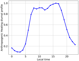
Figure 3Diurnal profiles of the anthropogenic heat flux in Paris for February and March 2014 constructed from traffic emission data for our study.
Furthermore, as in Lian et al. (2018), thanks to the fine spatial resolution of CORINE Land Cover data, we calculate the urban fraction for each 1 km × 1 km grid cell of the CHIMERE simulation domain. This fraction is used to modulate the anthropogenic heat flux at each model grid cell when the SLUCM is activated. Indeed, the anthropogenic heat flux computed by the urban canopy model is proportionate to the urban land cover (urban fraction); if this parameter is equal to 1, the entire anthropogenic heat flux settled in the SLUCM is taken into account. Hence, we are able to use a consistent urban canopy model parameterization for the city of Paris.
Concerning the configuration of the urban landscape geometry, we obtain the building heights and the road widths from the BD TOPO (version 3) database (https://geoservices.ign.fr/bdtopo, last access: 28 October 2024); roof widths follow Kim et al. (2013) and Thouron et al. (2017). The analysis of several test simulations allowed us to find the most suitable geometry configuration for each of the three urban categories from CORINE Land Cover data. All these parameters are presented in Table 2, and the unmentioned parameters are based on Kusaka et al. (2001).
The downtown Paris area is classified as “High urban density” in the CORINE Land Cover dataset. The Parisian suburban area is mainly classified as “Low urban density”, and finally, all the other urban areas corresponding to industrial areas, large shopping centers, highways, or railway networks are classified as “Commercial/industrial/transport”.
Without the urban canopy model, WRF calculates friction velocities that are often lower than the limit value of 0.01 m s−1. As mentioned earlier, this leads to unrealistic high-concentration peaks for all the studied pollutants modeled with MUNICH (NO2, PM2.5, and PM10). With the SLUCM configuration described in Table 2, the friction velocity remains consistently above 0.01 m s−1 in cells classified as urban areas.
In the context of our investigation, our findings suggest that raising the friction velocity threshold to 0.1 m s−1 within the surface layer scheme effectively mitigates the occurrence of unrealistic peaks in the simulation. However, it is noteworthy that this threshold value is insufficient for accurately representing the elevated pollutant concentrations observed during air pollution episodes. Our study underscores the significance of incorporating an urban model within the Weather Research and Forecasting (WRF) framework, which introduces an additional anthropogenic heat flux. This appears particularly crucial for locations near highways where traffic-related emissions are substantially high.
3.1.4 Configuration of the chemistry
The numerical algorithms used in the CHIMERE subgrid-scale and the CHIMERE MUNICH approaches are not exactly the same, but they lead to the same background concentrations. For example, simulated background concentrations for PM2.5 have a correlation greater than 0.99 at every background station, and the bias is on the order of 0.1 µg m−3.
For CHIMERE and MUNICH simulations, the same configuration of SSH-aerosol is used. Both simulations use the same chemical module for gas chemistry, the MELCHIOR2 mechanism (Derognat et al., 2003; Carter, 1990), and the H2O (“hydrophilic/hydrophobic organic”) reduced mechanism for the SOA (secondary organic aerosol) formation from VOCs (volatile organic compounds; Couvidat et al., 2012). For both models, the time integration of the gas-phase chemistry is solved explicitly and is not based on a stationarity assumption, which means that different timescales can be taken into account.
In addition, the time evolution of particulate concentrations in SSH-aerosol takes coagulation and condensation/evaporation of aerosols into account. The latter process is modeled based on a thermodynamic equilibrium hypothesis as detailed in Sartelet et al. (2020). For this study, CHIMERE and MUNICH use 10 particle size sections with the following cut-off diameters: 0.01, 0.022, 0.048, 0.107, 0.235, 0.516, 1.136, 2.5, 5, 10, and 40 µm. We do not account for nucleation in our simulations, because we focus our analysis on particle mass concentration indicators, especially PM2.5, which is hardly sensitive to this process (Sartelet et al., 2022).
3.2 Local-scale simulation setup
3.2.1 The street-network model MUNICH
The road segments of the street network considered in this study were originally defined by Airparif, the Île-de-France air quality agency. For each road segment, Airparif assigns emission fluxes for the main pollutants emitted by road traffic. To assign mean width and mean buildings' height to each road segment of the network, we use the national BD TOPO database (https://geoservices.ign.fr/bdtopo). The mean street width is calculated by adding the mean road width (also from the BD TOPO database) and the sidewalk width (public open-access data available at https://opendata.apur.org/datasets/Apur::trottoir/, last access: 28 October 2024). We combined streets that have intersections that are less than 4.5 m apart. The final street network comprises 4655 streets and extends over the city of Paris and its nearby suburbs. The minimum building height in the entire network is established at 1 m.
The emissions assigned to the streets are given as annual totals. We applied average temporal profiles provided by Airparif to obtain hourly fluxes for the period of the study. The period-averaged NO2 emission fluxes over the road network are shown in Fig. 1d and highlight the busiest roads. Also shown on the same map are the monitoring sites of the Airparif network (detailed in Sect. 3.3).
3.2.2 The Subgrid method
The subgrid-scale model is fully embedded in CHIMERE; therefore, both models share the same configuration. As explained in Sect. 2.1, grid cells split into several subgrid environments. Here, we split all cells containing a monitoring station into two subgrid environments: “roads”, including all emissions from the road network assuming that they are emitted over the grid-cell area fraction corresponding to the road network, and “other”, including all other emissions assumed to be released over the rest of the grid-cell area. The approach is applied only to cells containing a traffic station, representing a total of 8 cells. Their locations within the grid are illustrated in Fig. 1d.
3.3 Measurement stations and land use
Since our goal is to compare two methods that are able to represent pollutant concentrations at the street scale, we will essentially discuss comparisons at traffic stations (displayed in black in the Fig. 1). Model evaluation focuses on NOx, NO2, and PM2.5 concentrations. Not all stations measure these three pollutants. PM2.5 observations are only taken at two traffic stations, AUT and BP_EST, close to the ring road. The RN2 station is outside the city on a busy road, while the rest are within the city with lower emissions. Two key features of this measurement network should be noted:
-
BP_EST and SOULT are situated within the same grid cell, sharing identical emission data in the Subgrid approach, thus yielding equivalent results from this method. This is the same case for the stations HAUS and OPERA.
-
BASCH and OPERA are two stations situated on a roundabout. Assigning a specific street to these stations is not feasible. Some results are, however, discussed in Sect. 4.1.2.
The pixels in the CORINE Land Cover database around the station AUT were originally assigned to the category “Cropland/natural vegetation mosaic” due to their proximity to the Bois de Boulogne public park. However, this observation site is much more influenced by the vicinity of a road junction and the ring road. It was therefore decided to modify the category assigned to the pixel containing the site to “Commercial/industrial/transport”. The modification significantly enhanced the results of the MUNICH local model simulation for this site. Prior to this correction, MUNICH generated peaks of NOx approaching almost 4500 µg m−3 and peaks of fine particles exceeding 800 µg m−3, results that were deemed unrealistic. Notably, all stations, except AUT and RN2, are situated within model grid cells categorized as “high urban density” according to the CORINE urban classification (detailed in Sect. 3.1.3). AUT and RN2 are located within a model grid cell classified as “Commercial/industrial/transport”.
The concentrations of NOx, NO2, and PM2.5 simulated with MUNICH and Subgrid methods are compared with observations from measurement stations characterized by very dense traffic (BP_EST, AUT, and RN2) and from stations located inside the city (CELES, ELYS, HAUS, BONAP, and SOULT), where pollutant emissions from traffic are lower. For these stations, we analyze the impact of (i) differentiating emissions and aspect ratios () and (ii) the daily concentration profile for each approach. The specific cases of stations BASCH and OPERA are discussed independently in Sect. 4.1.2.
4.1 Evaluation against observations at traffic sites
4.1.1 Global analysis
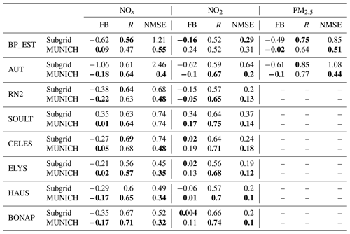
Model evaluation involves comparing the simulated concentrations with the observations through various statistical metrics that we deemed relevant to our analyses: the fractional bias (FB), the Pearson correlation (R), and the normalized mean square error (NMSE), which are described in Appendix A. The comparisons are done for hourly concentrations and for the entire simulation period. Table 4 shows model scores for NOx, NO2, and PM2.5 concentrations simulated with the two modeling methods.
For NOx concentrations, the fractional bias (FB) varies from −0.22 (RN2) to 0.09 (BP_EST) with MUNICH and from −1.06 (AUT) to 0.35 (SOULT) with the Subgrid method. The average of the FB for the studied measurement network (eight stations) is equal to −0.07 for MUNICH and −0.35 for the Subgrid method. For the two stations on the Paris ring road (BP_EST and AUT), the Subgrid approach significantly underestimates the concentrations with an FB of around −0.84. We observed that the Subgrid method significantly overestimates NOx concentrations at the SOULT station. An overarching problem with the description of emissions arises due to the heterogeneity between SOULT and BP_EST, located in the same cell. Indeed, this area is crossed by the heavily trafficked Paris ring road, which introduces significant urban spatial heterogeneity (see Fig. 4). This is extensively discussed in Sect. 4.2. The street-network model gives, in general, better performances than the Subgrid method for NOx. The correlation coefficient remains an exception, as both methods exhibit nearly identical performances, around 0.62.
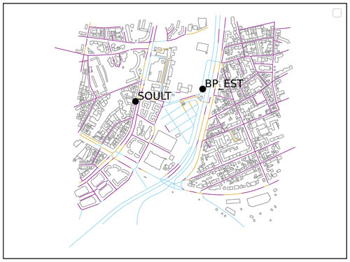
Figure 4The grid cell that contains the stations BP_EST and SOULT, displayed with the BD TOPO database: buildings are represented in gray, the open street in blue, the intermediate street in yellow, and the canyon street in purple.
For NO2 concentrations, the fractional bias (FB) varies from −0.1 (AUT) to 0.24 (BP_EST) with MUNICH and from −0.62 (AUT) to 0.34 (SOULT) with the Subgrid method. The average of the FB for the studied measurement network is equal to 0.08 for MUNICH and −0.07 for the Subgrid method. In contrast to NOx concentrations, MUNICH demonstrates an improvement in the correlation of approximately 8 % compared to the Subgrid approach. The average correlation for the street-network model is 0.67, while it is 0.59 for the Subgrid method. We also noted that for NO2 and NOx concentrations, the street-network model generates a lower NMSE for most of the studied stations. The superior performance of the Subgrid method for NO2 compared to NOx in terms of fractional bias is apparent. This distinction may be attributed to the regional component of NO2 being more prominent than that of NOx, which is more influenced by local traffic emissions.
The statistical analysis for PM2.5 is conducted solely on two stations situated along the Paris ring road (refer to Table 4). It is evident that MUNICH significantly outperforms the Subgrid approach for these two specific stations, albeit not in terms of correlation. The Subgrid method achieves an average correlation of 0.8, while MUNICH exhibits an average correlation of approximately 0.7 for the two stations. To complete this overview of the performances of each method, the summary of the criteria results from Herring and Huq (2018) for all the studied stations is shown in Appendix C.
The 2-month period under study includes a pollution episode from 5 to 17 March. When comparing the fractional bias and the NMSE of each method across different periods (during the pollution episode and outside it), no significant differences are observed between the two approaches for the three pollutants analyzed. The NMSE remains consistent throughout the entire period, and the fractional bias observed outside the air pollution episode is fairly similar to that calculated during the pollution episode (see Table C3 in Appendix C).
4.1.2 Analysis specific to stations
A substantial gas concentration disparity between the two approaches is evident throughout the entire period for AUT (see Fig. 5) and BP_EST. This pattern is also observed in PM2.5 concentrations. Notably, these are the only two stations in the measurement network located on the heavily trafficked Paris ring road. The Subgrid method provides concentrations at street level, but on average for an entire cell of 1 km × 1 km. The result provided by the Subgrid method should, therefore, be interpreted as an average on-road concentration for the different street segments located inside the grid cell. Considering, for instance, the grid cell containing the BP_EST station, the Subgrid method uses a single NO2 emission flux of 5.7 µg s−1 m−2 on average over the simulation period, representing a spatially averaged flux among all road segments located inside the grid cell. The NO2 emission flux for the road segment containing the BP_EST station, explicitly provided to MUNICH, is estimated equal to 18.8 µg s−1 m−2. It is therefore not surprising that the concentration simulated with the Subgrid method underestimates concentrations at the BP_EST station. Symmetrically, the common NO2 emission flux used by the Subgrid method for the SOULT station, located in the same grid cell than BP_EST, overestimates the one given for the street containing this station, equal to 2.49 µg s−1 m−2. An overestimation of the concentrations can therefore be expected. This a priori qualitative analysis, also valid for NOx and PM2.5 emission fluxes, appears to be confirmed by the comparison between concentrations simulated by the Subgrid method and observations, particularly for NOx: the fractional bias (FB) stands at −0.62 at the BP_EST station, and it equals 0.35 at the SOULT station. A similar trend is noted for NO2, albeit less pronounced at BP_EST, with an FB of −0.16, and still evident at SOULT with an FB of 0.34. While observation data for fine particles on SOULT are unavailable, simulations for BP_EST indicate an underestimation with an FB of 0.49.
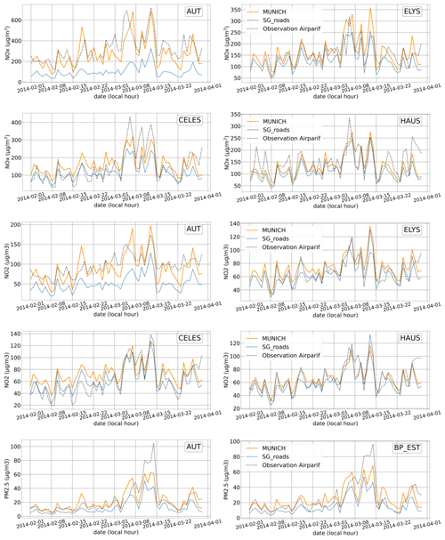
Figure 5Daily average concentrations observed (black dot), simulated by MUNICH (in orange), and simulated by the Subgrid method (in blue) over 2 months at some of the most representative stations in the Airparif measurement network for NOx, NO2, and PM2.5 concentrations.
Table 3Characteristics of traffic proximity sites in the Airparif observation network. Note: n/a represents not applicable.
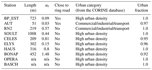
Table 4Statistical indicators for comparison of hourly concentrations of NOx, NO2 and PM2.5 from February to March 2014 at traffic stations. Bold numbers indicate the best performances.
For the other stations within the city, the differences between the two approaches are less noticeable. The simulated concentrations generated by each method appear nearly identical for stations such as HAUS and BONAP (the former station is depicted in Fig. 5). However, the discrepancies are slightly more important for CELES and ELYS. Regarding NOx concentrations, MUNICH performs better than the Subgrid method for these two stations throughout the entire study period (see Table 4), but this is not the case for NO2. CELES, located on the docks, is associated with a cell characterized by higher emission heterogeneity, which could contribute to the observed disparities between the approaches. In the case of ELYS, the station shares similarities in terms of traffic emissions with HAUS and BONAP. However, a crucial distinction lies in its aspect ratio, which is significantly lower (as detailed in Table 3). The impact of this aspect ratio on the observed discrepancies is described in Sect. 4.2.
Table 5Statistical indicators for comparison of hourly concentrations of NOx, NO2, and PM2.5 from February to March 2014 at traffic stations on a roundabout. MUNICH_1 represents the street providing the most accurate estimations of concentrations among the streets connected to the associated roundabout, while MUNICH_2 corresponds to the street with the least-accurate gas concentration estimations.
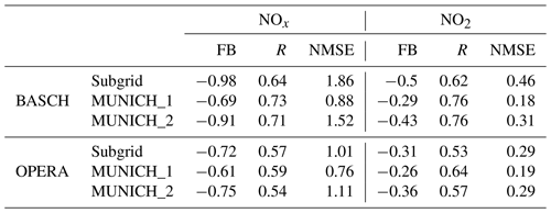
As mentioned above, the OPERA and BASCH measurement stations are located on roundabouts. The primary challenge in simulating pollutant concentrations at these stations comes from the uncertainty associated with the estimation of traffic emissions. Noticeably, the local congestion effects and the shutdowns and restarts that this entails are not explicitly taken into account to build the emission inventory. Consequently, there is a potential underestimation of traffic emissions at these locations. To further characterize this issue concerning MUNICH, we conducted an analysis of each street connected to one of these roundabouts, identifying two streets: one yielding the best statistical indicators and another producing the worst. Table 5 showcases significant fractional biases for each approach at the two stations. For OPERA, the performance of the Subgrid approach falls between the street with the best results (MUNICH_1 in Table 5) and the one with the least-accurate gas concentration (MUNICH_2). However, a different scenario unfolds for BASCH, where the Subgrid method even performs worse than the street that is generating the least-accurate results. The main distinction between these two cells lies in the fact that the urban environment surrounding OPERA is more homogeneous than that surrounding BASCH.
Through this first analysis, it becomes clear that the disparities between the approaches vary greatly depending on the location of the stations. These stations are characterized by different emissions and different types of buildings. These aspects are further explored in the subsequent sections.
4.2 Impact of differentiated emissions and aspect ratio
By definition, the Subgrid method is supposed to represent a portion of a neighborhood, whereas the MUNICH model generates concentrations for every single street. To emphasize the impact of this conceptual difference, we compare in Fig. 6 the concentrations simulated with MUNICH for each street to the corresponding CHIMERE Subgrid grid cell (area of 1 km2) but also with the mean of all the streets of the MUNICH road network located inside this CHIMERE grid cell. This new averaged MUNICH output is noted as MUNICH_cell in Fig. 6. The fractional bias generated by MUNICH_cell minus Subgrid (depicted by the blue bar plot) is significantly lower than that of MUNICH minus Subgrid (green bar plot) at all stations for each pollutant. This outcome underscores the similarity in the average behavior of each method.
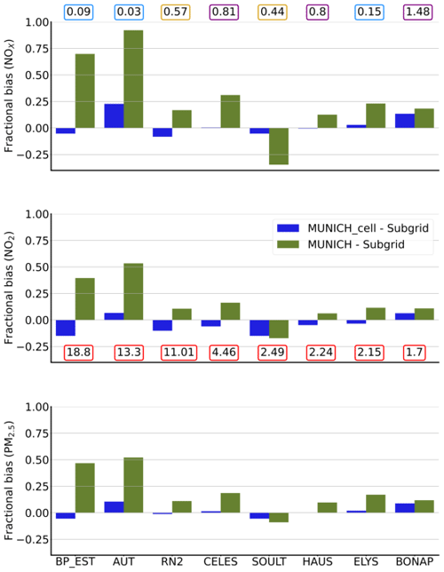
Figure 6Comparison of the fractional biases between MUNICH and the Subgrid method (in green) and between the mean of all the street segments computed by MUNICH inside the cell (MUNICH_cell) and the Subgrid method (in dark blue) for concentrations of NOx, NO2, and PM2.5 for each traffic station. The stations are ordered (from left to right) from the station with the highest NO2 emissions (BP_EST) to the station with the lowest NO2 emissions (BONAP). Below the middle panel, the NO2 mean emission values (in µg s−1 m−2) over the 2 studied months are displayed. Above the top panel, the aspect ratio associated with each station is indicated: light blue indicates that the stations are located in a wide street, yellow indicates that they are in an intermediate street, and purple indicates that they are inside a narrow canyon.
Stations located in cells intersected by the Paris ring road exhibit the most substantial difference between the two approaches for NOx, NO2, and PM2.5. Additionally, when examining AUT and RN2, two stations with comparable emissions (13.3 and 11.0 µg s−1 m−2, respectively), their FBs significantly differ for the three pollutants. The observed discrepancies are then not solely attributable to traffic emission levels, and this justifies the performance disparities as a consequence of urban heterogeneity tied to emissions and urban topography.
It is interesting to quantify the influence of these two factors separately for the differences observed. However, it is worth noting that they are not entirely independent: in our domain, a highway with substantial traffic emissions generally corresponds to a broad and open road. Moreover, in MUNICH, the impact of the aspect ratio, αr, on street concentrations is more pronounced for streets with high emissions than for those with low emissions. Additionally, a third factor could impact these discrepancies. Because the Subgrid method only has information about the street area, we could expect some contribution from the wind direction. Its influence on the discrepancies observed between the approaches has been studied and does not reveal any significant impact in our case. But this could be due to the fact that the wind direction barely changes over the studied period, making it challenging to analyze its influence.
As expected, through an extension of the analysis on all the streets in the cells calculated by the Subgrid method (see Appendix B), it is easy to show that emission heterogeneity is an important factor in the discrepancies observed between the two approaches.
However, as observed in Fig. B1b, comparing concentration differences with the aspect ratio of the street, the aspect ratio seems to be not very relevant. This can be explained by the absence of a direct use of the aspect ratio in the Subgrid approach, which only considers the surface area of the street.
Consequently, further data are required to ascertain the impact of street aspect ratios on the differences observed between the two approaches. We conducted four additional MUNICH simulations, each with an identical aspect ratio for the entire street network: one with αr = 0.25, another with αr = 0.5, a third with αr = 1.0, and a fourth with αr = 1.5. These values are chosen to cover the range of cases observed in our network. The heights and widths of the streets have been resized to maintain their volume following Kim et al. (2022a). Figure 7 presents the results of these investigations and underscores the importance of αr.
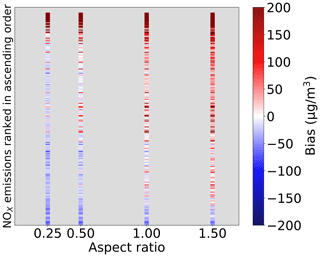
Figure 7Bias between four MUNICH simulations with identical αr with the Subgrid method for NOx as a function of αr (the x axis) and the average emissions of MUNICH (the y axis, without units, corresponding to the streets ranked in ascending order of emissions) of all the streets (points) for all the cells calculated by the Subgrid method in February and March 2014.
It logically shows that for a given emission level, the FB between MUNICH and the Subgrid method increases with αr due to the increase in MUNICH concentrations. However, this increase is very limited for the streets with low emissions (below ∼ 1 µg s−1 m−2), since for such streets the concentration level is mainly driven by background concentrations.
Regarding NOx, the MUNICH simulation with the highest αr (1.5) yields higher concentrations than the Subgrid method for most streets, while the opposite behavior is observed for the MUNICH simulation with the lowest αr (0.25). The average biases over the streets between the Subgrid method and the different MUNICH simulations are 5, 34, 92, and 153 µg m−3 for αr, respectively, equal to 0.25, 0.5, 1.0, and 1.5. The same trend on average biases is observed for NO2 and PM2.5, with values ranging from 3 µg m−3 with αr = 0.25 to 37 µg m−3 with αr = 1.5 for NO2 and from 0.7 to 8 µg m−3 for PM2.5.
The MUNICH simulation with αr = 0.25 closely mirrors the Subgrid simulation for NOx that can be approximately considered as a passive tracer with a linear behavior with respect to emissions. Both simulations rely on the same total traffic emissions, with only their spatial distribution changing. In other words, this simulation most accurately replicates the average dispersion conditions observed with the Subgrid method compared to the other simulations.
Following this observation, the biases between the Subgrid simulation and the MUNICH simulation with αr = 0.25 can be used to approximately assess the influence of the representation of emission heterogeneity in the difference between the two methods. The biases range from −39 to 122 µg m−3, with a standard deviation equal to 17 µg m−3 for cells within the city. However, we notice that for cells with heterogeneous emissions (including highways), this standard deviation is clearly higher (170 µg m−3), with biases ranging from −82 to 922 µg m−3.
If we carry out the same analysis but instead of using the Subgrid simulation we compute the bias between the original MUNICH simulation and the one with αr = 0.25, we can then approximately assess the impact of the aspect ratio. For cells within the city, we obtain a standard deviation of 21 µg m−3, with values ranging from −152 to 89 µg m−3. Once again, the biases computed for cells intersected by highways are generally higher, with a standard deviation reaching 93 µg m−3, ranging from −152 to 386 µg m−3.
Firstly, we noticed that the influence of both the aspect ratio and emission heterogeneities are more pronounced in cells intersected by highways. Secondly, although their impacts are fairly equivalent on city center cells, we observed for the cells intersected by highways that the impact of emission heterogeneity is considerably more significant than that of the aspect ratio. This is reflected in the standard deviation, which is almost twice as large for the influence of emissions compared to the aspect ratio.
The previous analysis performed on NOx cannot be directly extended to NO2 and PM2.5 due to the nonlinearity of the chemistry and its impact on the secondary contribution to the concentrations. Within the comparison between the Subgrid method and the four different MUNICH simulations with constant αr, the relative variation of simulated concentrations is greater in the case of NOx than for NO2 and PM2.5. For instance, the fractional bias between the original MUNICH simulation and the one with αr = 0.25 varies from −0.7 to 1.5. In comparison, the corresponding fractional bias for NO2 and PM2.5 ranges from −0.2 to 1.1. The NO2 and PM2.5 concentrations calculated by MUNICH are less affected by the street aspect ratio, because the concentrations of these pollutants have a more significant background component compared with NOx, whose concentration spatial patterns are more marked by road traffic emissions.
The influence of the local description of emissions is undoubtedly very important in the difference in performances of the two studied models, especially for highways where the Subgrid method is not capable of using sufficiently accurate emissions. Regarding the aspect ratio of the street, its impact on the disparities observed between each method is lower but present.
4.3 Analysis of daily cycles
The aspect ratio of the street and emissions play an important role in the differences observed between the approaches. Nevertheless, the impact of these factors may vary depending on the specific time periods under analysis. The subsequent section delves into the distinctions observed throughout different times of the day.
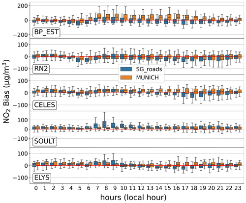
In Fig. 8, 2-month averaged 24 h profiles of the bias between observed and simulated concentrations for NOx and NO2 at AUT, HAUS, and BONAP stations are presented. The central horizontal bar in the boxplots represent the median of all the biases during the 2 months for a specific hour. The other horizontal bars represent the different quartiles. These three measurement stations have been selected to represent various cases highlighted in the previous section: AUT is situated in an urban zone characterized by a significant emission heterogeneity, HAUS is located in an area with more homogeneous emissions, and finally BONAP shares similarities with HAUS but is positioned on a street notably narrower than other ones around.
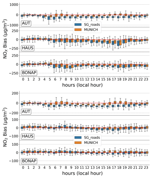
Figure 8Daily profiles of the bias (in µg m−3) between observed and simulated concentrations for the period of February–March 2014 for NOx and NO2 concentrations.
In areas with significant emission heterogeneity (such as AUT and BP_EST), the Subgrid approach underestimates gas concentrations at each hour of the day, with the discrepancies compared to MUNICH being particularly marked during the concentration peaks corresponding to rush hours (from 05:00 to 09:00 LT and from 17:00 to 20:00 LT). This pattern is also observed for PM2.5 concentrations. In areas with less emission heterogeneity (HAUS and BONAP), the two methods exhibit alternating periods of overestimation and underestimation of NOx and NO2 concentrations throughout the day, with the dispersion of the bias of each approach being quite similar. Specifically, the spreads of these biases (the difference between the maximum and minimum bias) for the two methods remain fairly similar for a given hour of the day. This underscores the similarity in the daily variability of the methods. The other stations are displayed in Appendix E.
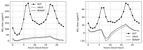
Figure 9Daily profiles of the bias (in µg m−3) between MUNICH and Subgrid simulations over the period of February–March 2014 for NOx and NO2 concentrations.
Figure 9 shows the averaged 24 h profiles of the bias between MUNICH and the Subgrid approach at each hour of the day for the same three stations. It illustrates that the discrepancies between the two approaches become more pronounced at certain times of the day. These differences are minimal during nighttime and escalate with traffic. Regarding NOx concentrations, the bias between the two methods remains positive and increases slightly throughout daylight hours. This indicates that for these streets MUNICH retains traffic emissions for longer than the Subgrid approach. Conversely, for NO2 concentrations, the sign of the bias varies throughout the day. While in most cases the street-network model generates higher concentrations of NO2 than the Subgrid method, the latter generates higher concentrations during the morning. It is noteworthy that all the other stations (apart from AUT and BP_EST) behave in the same way as HAUS and BONAP, as shown in Fig. 9.
At the end of the night, the O3 concentrations of Subgrid are higher than those of MUNICH. This appears consistent with higher exchange between these streets and the background environment in the Subgrid method (αr ∼ 0.25) compared to MUNICH. The peak in morning traffic emissions starts to bring NOx while the atmospheric boundary layer is not fully developed; the titration of O3 by NO then leads to higher NO2 chemical production in the Subgrid method. Around 07:00 LT (local time), the O3 concentrations are very similar in both models, but the development of the boundary layer then brings more O3 in the Subgrid method. This allows the chemistry production of NO2 to overcompensate during some hours for the greater dilution of the Subgrid method.
The daily profiles confirm that the representation of emission heterogeneity is the main factor contributing to the differences observed between the two models. These differences are more pronounced during the daylight and may vary depending on the moment of the day.
In the current paper, we compared two methods to simulate street-level pollutant concentrations of NOx, NO2, and PM2.5 with observations at traffic measurement stations. The simulations are performed over Paris during a winter period (February and March 2014). The first approach, the Subgrid method, is a statistical method capable of disaggregating emissions of different sectors (traffic, residential, park, etc.) inside a grid cell. In our case, we subdivide the cells where there are traffic stations into two environments in order to concentrate the traffic emissions on a road surface. The second approach is the MUNICH model, which is based on a street-network approach. The considered network in MUNICH is composed of 4655 streets and represents the city of Paris and its close suburbs. These two methods make use of identical emissions, meteorological data, and background concentrations.
An urban canopy model (the SLUCM) has been applied in the WRF model to generate the meteorological data used by each method. We integrated three different urban categories and the urban fraction per grid cell from the CORINE Land Cover database in the geographic data file used by the WRF model. The simulations carried out as part of this study confirm the need to represent the anthropogenic sensible heat flux in the SLUCM for a winter period, which comes mainly from traffic, domestic energy, and human metabolism. These adjustments significantly influence the friction velocity and improve the background concentration simulated by the CHIMERE model and the performance of MUNICH.
While the street-network approach respects all the strictest criteria for the entire studied measurement network for NOx, NO2, and PM2.5, this is not the case for the Subgrid method. This latter method failed to correctly represent gas and fine-particle concentrations at stations located in urban areas with important spatial or temporal emission heterogeneity. For stations situated in the city center of Paris, MUNICH exhibits a lower fractional bias relative to observations (approximately −0.06) for NOx concentrations compared to the Subgrid method (−0.28), but the results concerning NO2 concentrations are more similar.
The most significant differences observed between the two approaches concern cells containing highly trafficked roads. These disparities are not directly attributed to the elevated emissions in these areas but are influenced by the presence of the Paris ring road (highway), which substantially alters the urban landscape, leading to heterogeneous emissions and varying building dimensions. We proposed an analysis of the respective role of emission and topography heterogeneities. Those linked to emissions appear to generate a larger range of bias values between the two methods than those linked to topography in urban areas including the Paris ring road. In the city center of Paris, both aspects appear to have a similar impact.
The analysis of the daily cycles reveals that the discrepancies between the approaches are more pronounced during rush hours. At the city center stations, which are characterized by fairly homogeneous emissions, we noted in the morning that the Subgrid method can generate higher NO2 concentrations than MUNICH due to higher ozone import.
This paper has identified potential areas for improvement in each of the local approaches: the robustness of the street-network model could be improved by a better representation of local meteorology, and applying the Subgrid method with a more diverse range of traffic area zones could enhance its performance in cells containing highways. Finally, these results offer encouraging prospects for a potential dynamic coupling between MUNICH and the coupled model CHIMERE-WRF. In a future study, the pollution transfers between local and regional scales will be enhanced through the development of a dynamic coupling (a two-way nesting) between the CHIMERE and MUNICH models.
The subsequent equations present the definitions of the statistical indicators employed in this paper, with o representing observations, s representing simulation data, and n representing the number of observations.
-
Fractional bias (range between −2 and 2, perfect value: 0):
-
Pearson correlation (range between −1 and 1, perfect correlation: 1):
-
Spearman correlation, computed as the Pearson correlation applied to the ranks of the pairs of values compared (range between −1 and 1, perfect correlation: 1):
-
Normalized mean square error (range higher or equal to 0, perfect value: 0):
-
FAC2 is the proportion of data that meets the criteria (range between 0 and 1, perfect value: 1):
-
Geometric variance (range higher or equal to 1, perfect value: 1):
The strong correlation between the emissions and the disparities observed between MUNICH and the Subgrid method is confirmed by Fig B1a in Appendix B. The cell containing a part of the Paris ring road, leading to a wide range of emission values, presents a significantly greater range of bias values than the cell inside the city (illustrated by Fig. B1b in Appendix B). Indeed, we observed that for stations near the Paris ring road, namely, BP_EST, AUT, and RN2, the minimum fractional bias averages −0.61, while the maximum reaches 1.08. In contrast, for stations within the city, the fractional bias ranges between −0.29 and 0.53 on average. This observation confirms that the discrepancies between the approaches are significantly less pronounced in areas with a more homogeneous distribution of emissions compared to those adjacent to highways, which introduce heterogeneous emissions.
In order to quantify the impact of emissions on the differences observed between the two studied approaches, Spearman's correlation defined in Appendix A is used. Spearman's rank correlation coefficient (defined in Appendix A) between (1) the FBs in the mean concentrations (for the 2 months studied) calculated by the two approaches and (2) the differences, Ediff(i), between the local emission in street i (Ei) and the average of emissions over the Ns streets in the corresponding cell (weighted by street surfaces ) is used to quantify the strength of the relationship. Ediff(i) is then defined as
For NOx, NO2, and PM2.5, the coefficients are 0.88, 0.85, and 0.87, respectively. These values confirm a significant correlation (potentially nonlinear) between the emission heterogeneity and the observed disparities between the modeling approaches.
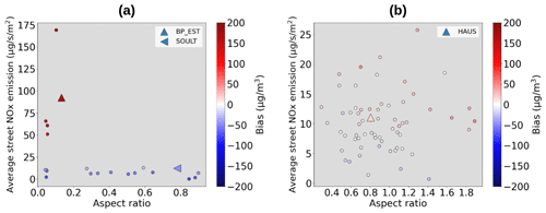
Figure B1Bias between MUNICH and the Subgrid method for NOx, as a function of αr (x axis), and the average emissions of MUNICH (y axis, in µg s−1 m−2) for all the streets (points) within a cell, over February and March 2014. The left panel shows the results for the cell containing stations BP_EST and SOULT (a), which includes part of the Paris ring road. The right panel shows the results for the cell containing HAUS (b), located within the city.
The tables below summarize whether each method adheres to the various criteria outlined by Herring and Huq (2018). An “O” indicates that the criteria is respected, while an “X” signifies rejection. “Sc” represents the strict criterion, which is the most stringent, and “Lsc” corresponds to the less strict criterion. The statistical indicator NMSE is not displayed in this appendix as it is not relevant in the current paper. Both approaches meet the criteria described by the normalized mean squared error (NMSE) for all the traffic stations.
Table C1Validation of the criterion from Herring and Huq (2018) on all the traffic stations for NOx and NO2.
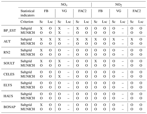
Table C2Validation of the criterion from Herring and Huq (2018) on all the traffic stations for PM2.5.
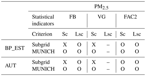
Table C3Comparison of the mean of the normalized mean square error (NMSE) and the fractional bias (FB) of all the stations during a normal period (NP) and during the air pollution episode (APE) for NOx, NO2 (at eight stations), and PM2.5 concentrations (at two stations), simulated by the Subgrid method and MUNICH.

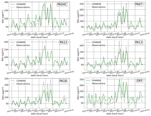
Figure D1Daily average concentrations observed (black dot) and simulated by CHIMERE (in green) over 2 months, at some measurement stations, for NOx concentrations.
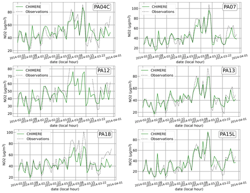
Figure D2Daily average concentrations observed (black dot) and simulated by CHIMERE (in green) over 2 months, at some measurement stations, for NO2 concentrations.
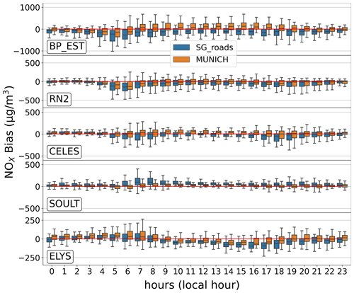
Figure E1Daily profiles of the bias (in µg m−3) between observed and simulated concentrations for the period of February–March 2014 for NOx concentrations.
The CHIMERE source code and its documentation, as well as the source code for the WRF model (version 3.7), are available at https://doi.org/10.14768/8afd9058-909c-4827-94b8-69f05f7bb46d (Menut et al., 2020, 2021). The MUNICH v2.0 model source code may be accessed at https://doi.org/10.5281/zenodo.6167477 (Kim et al., 2022b, a).
The observation data from Airparif for 2014 are publicly available and can be downloaded from: https://www.geodair.fr/donnees/export-advanced (Airparif, 2024). The meteorological and background data required by MUNICH (CHIMERE outputs) and the emissions data used by both models are provided on Zenodo at https://doi.org/10.5281/zenodo.14164944 (Squarcioni, 2024). The CORINE Land Cover 2018 dataset used in this study is available at https://doi.org/10.2909/960998c1-1870-4e82-8051-6485205ebbac (European Union's Copernicus Land Monitoring Service, 2020).
AS wrote the draft of the manuscript with contributions from YR and MV. AS, YR, and MV performed the analysis. AS and MV constructed the street network with contributions from FD. AS conducted the CHIMERE, WRF, and SSH-aerosol simulations with contributions from MV, LL, YK, and KS. AS conducted the MUNICH simulations with contributions from YR, YK, KS, and LL. RV provided the network emission data. AS, YR, MV, YK, KS, LL, and FD reviewed the final manuscript.
The contact author has declared that none of the authors has any competing interests.
Publisher's note: Copernicus Publications remains neutral with regard to jurisdictional claims made in the text, published maps, institutional affiliations, or any other geographical representation in this paper. While Copernicus Publications makes every effort to include appropriate place names, the final responsibility lies with the authors.
This article is part of the special issue “Air quality research at street level – Part II (ACP/GMD inter-journal SI)”. It is not associated with a conference.
The authors would like to thank Airparif for the discussions and emissions provided. We thank the TGCC (Très Grand Centre de Calcul du CEA); this work was carried out using the HPC high-performance computing resources of GENCI TGCC under grant no. A0130110274.
Alexis Squarcioni's PhD grant is funded by the Île-de-France region as part of the “Paris Region PhD” program (grant no. 20007179) and the Airparif air quality agency (grant no. C23/0946).
This paper was edited by Franziska Aemisegger and reviewed by two anonymous referees.
Airparif: L'observatoire de la qualité de l'air en Île-de-France, GeoD'air [data set], https://www.geodair.fr/donnees/export-advanced (last access: 20 December 2024), 2024. a
Allen, L., Lindberg, F., and Grimmond, C. S. B.: Global to city scale urban anthropogenic heat flux: model and variability, Int. J. Climatol., 31, 1990–2005, https://doi.org/10.1002/joc.2210, 2010. a, b
Azmi, W. N. F. W., Pillai, T. R., Latif, M. T., Koshy, S., and Shaharudin, R.: Application of land use regression model to assess outdoor air pollution exposure: A review, Environmental Advances, 11, 100353, https://doi.org/10.1016/j.envadv.2023.100353, 2023. a
Beevers, S. D., Kitwiroon, N., Williams, M. L., and Carslaw, D. C.: One way coupling of CMAQ and a road source dispersion model for fine scale air pollution predictions, Atmos. Environ., 59, 47–58, 2012. a
Benavides, J., Snyder, M., Guevara, M., Soret, A., Pérez García-Pando, C., Amato, F., Querol, X., and Jorba, O.: CALIOPE-Urban v1.0: coupling R-LINE with a mesoscale air quality modelling system for urban air quality forecasts over Barcelona city (Spain), Geosci. Model Dev., 12, 2811–2835, https://doi.org/10.5194/gmd-12-2811-2019, 2019. a
Berchet, A., Zink, K., Oettl, D., Brunner, J., Emmenegger, L., and Brunner, D.: Evaluation of high-resolution GRAMM–GRAL (v15.12/v14.8) NOx simulations over the city of Zürich, Switzerland, Geosci. Model Dev., 10, 3441–3459, https://doi.org/10.5194/gmd-10-3441-2017, 2017. a
Berkowicz, R.: OSPM – A Parameterised Street Pollution Model, Environ. Monit. Assess., 65, 323–331, https://doi.org/10.1023/a:1006448321977, 2000. a
Briant, R., Tuccella, P., Deroubaix, A., Khvorostyanov, D., Menut, L., Mailler, S., and Turquety, S.: Aerosol–radiation interaction modelling using online coupling between the WRF 3.7.1 meteorological model and the CHIMERE 2016 chemistry-transport model, through the OASIS3-MCT coupler, Geosci. Model Dev., 10, 927–944, https://doi.org/10.5194/gmd-10-927-2017, 2017. a
Cambridge Environmental Research Consultants: ADMS 3 User Guide, Cambridge Environmental Research Consultants, Cambridge, https://www.cerc.co.uk (last access: 19 December 2024), 2001. a
Carter, W. P. L.: A detail mechanism for the gas-phase atmospheric reactions of organic compounds, Atmos. Environ. A-Gen., 24, 481–518, https://doi.org/10.1016/0960-1686(90)90005-8, 1990. a
Couvidat, F. and Sartelet, K.: The Secondary Organic Aerosol Processor (SOAP v1.0) model: a unified model with different ranges of complexity based on the molecular surrogate approach, Geosci. Model Dev., 8, 1111–1138, https://doi.org/10.5194/gmd-8-1111-2015, 2015. a
Couvidat, F., Debry, E., Sartelet, K., and Seigneur, C.: A hydrophilic/hydrophobic organic (H2O) aerosol model: Development, evaluation and sensitivity analysis, J. Geophys. Res.-Atmos., 117, D10304, https://doi.org/10.1029/2011jd017214, 2012. a, b
Derognat, C., Beekmann, M., Baeumle, M., Martin, D., and Schmidt, H.: Effect of biogenic volatile organic compound emissions on tropospheric chemistry during the Atmospheric Pollution Over the Paris Area (ESQUIF) campaign in the Ile‐de‐France region, J. Geophys. Res.-Atmos., 108, 8560, https://doi.org/10.1029/2001jd001421, 2003. a
Dons, E., Van Poppel, M., Kochan, B., Wets, G., and Int Panis, L.: Modeling temporal and spatial variability of traffic-related air pollution: Hourly land use regression models for black carbon, Atmos. Environ., 74, 237–246, https://doi.org/10.1016/j.atmosenv.2013.03.050, 2013. a
Dupont, J.-C., Haeffelin, M., Badosa, J., Elias, T., Favez, O., Petit, J., Meleux, F., Sciare, J., Crenn, V., and Bonne, J.: Role of the boundary layer dynamics effects on an extreme air pollution event in Paris, Atmos. Environ., 141, 571–579, https://doi.org/10.1016/j.atmosenv.2016.06.061, 2016. a
EEA: Europe's air quality status 2023, EEA Briefing, Publications Office, https://doi.org/10.2800/59526, 2023. a
European Union's Copernicus Land Monitoring Service: CORINE Land Cover 2018 (raster 100 m), Europe, 6-yearly – version 2020_20u1, European Union's Copernicus Land Monitoring Service [data set], https://doi.org/10.2909/960998c1-1870-4e82-8051-6485205ebbac, 2020. a
Fuzzi, S., Baltensperger, U., Carslaw, K., Decesari, S., Denier van der Gon, H., Facchini, M. C., Fowler, D., Koren, I., Langford, B., Lohmann, U., Nemitz, E., Pandis, S., Riipinen, I., Rudich, Y., Schaap, M., Slowik, J. G., Spracklen, D. V., Vignati, E., Wild, M., Williams, M., and Gilardoni, S.: Particulate matter, air quality and climate: lessons learned and future needs, Atmos. Chem. Phys., 15, 8217–8299, https://doi.org/10.5194/acp-15-8217-2015, 2015. a
Guenther, A. B., Jiang, X., Heald, C. L., Sakulyanontvittaya, T., Duhl, T., Emmons, L. K., and Wang, X.: The Model of Emissions of Gases and Aerosols from Nature version 2.1 (MEGAN2.1): an extended and updated framework for modeling biogenic emissions, Geosci. Model Dev., 5, 1471–1492, https://doi.org/10.5194/gmd-5-1471-2012, 2012. a
Hamer, P. D., Walker, S.-E., Sousa-Santos, G., Vogt, M., Vo-Thanh, D., Lopez-Aparicio, S., Schneider, P., Ramacher, M. O. P., and Karl, M.: The urban dispersion model EPISODE v10.0 – Part 1: An Eulerian and sub-grid-scale air quality model and its application in Nordic winter conditions, Geosci. Model Dev., 13, 4323–4353, https://doi.org/10.5194/gmd-13-4323-2020, 2020. a
Hatzopoulou, M., Valois, M. F., Levy, I., Mihele, C., Lu, G., Minet, S. B. L., and Brook, J.: Robustness of Land-Use Regression Models Developed from Mobile Air Pollutant Measurements, Environ. Sci. Technol., 51, 3938–3947, 2017. a
Herring, S. and Huq, P.: A Review of Methodology for Evaluating the Performance of Atmospheric Transport and Dispersion Models and Suggested Protocol for Providing More Informative Results, Fluids, 3, 20, https://doi.org/10.3390/fluids3010020, 2018. a, b, c, d
Hood, C., MacKenzie, I., Stocker, J., Johnson, K., Carruthers, D., Vieno, M., and Doherty, R.: Air quality simulations for London using a coupled regional-to-local modelling system, Atmos. Chem. Phys., 18, 11221–11245, https://doi.org/10.5194/acp-18-11221-2018, 2018. a
Hooyberghs, H., De Craemer, S., Lefebvre, W., Vranckx, S., Maiheu, B., Trimpeneers, E., Vanpoucke, C., Janssen, S., Meysman, F., and Fierens, F.: Validation and optimization of the ATMO-Street air quality model chain by means of a large-scale citizen-science dataset, Atmos. Environ., 272, 118946, https://doi.org/10.1016/j.atmosenv.2022.118946, 2022. a
Hourdin, F., Musat, I., Bony, S., Braconnot, P., Codron, F., Dufresne, J.-L., Fairhead, L., Filiberti, M.-A., Friedlingstein, P., Grandpeix, J.-Y., Krinner, G., LeVan, P., Li, Z.-X., and Lott, F.: The LMDZ4 general circulation model: climate performance and sensitivity to parametrized physics with emphasis on tropical convection, Clim. Dynam., 27, 787–813, https://doi.org/10.1007/s00382-006-0158-0, 2006. a
Hunt, J. C. R., Holroyd, R. H., and Carruthers, D. J.: Preparatory Studies for a Complex Dispersion Model, Cambridge Environmental Research Consultants, Cambridge, https://admlc.com/wp-content/uploads/2014/09/admsrep.pdf (last access 18 December 2024), 1988. a
Jiménez, P. A., Dudhia, J., González-Rouco, J. F., Navarro, J., Montávez, J. P., and García-Bustamante, E.: A Revised Scheme for the WRF Surface Layer Formulation, Mon. Weather Rev., 140, 898–918, https://doi.org/10.1175/mwr-d-11-00056.1, 2012. a, b
Karl, M., Walker, S.-E., Solberg, S., and Ramacher, M. O. P.: The Eulerian urban dispersion model EPISODE – Part 2: Extensions to the source dispersion and photochemistry for EPISODE–CityChem v1.2 and its application to the city of Hamburg, Geosci. Model Dev., 12, 3357–3399, https://doi.org/10.5194/gmd-12-3357-2019, 2019. a
Kiesewetter, G., Borken-Kleefeld, J., Schöpp, W., Heyes, C., Bertok, I., Thunis, P., Bessagnet, B., Terrenoire, E., and Amann, M.: Modelling compliance with NO2 and PM10 air quality limit values in the GAINS model, Tech. Rep. Thematic Strategy on Air Pollution #9, International Institute for Applied Systems Analysis, https://previous.iiasa.ac.at/web/home/research/researchPrograms/air/policy/TSAP-Report-_9-v1_final-MA.pdf (last access: 2 November 2024), 2013. a
Kim, Y., Sartelet, K., Raut, J.-C., and Chazette, P.: Evaluation of the Weather Research and Forecast/Urban Model Over Greater Paris, Bound.-Lay. Meteorol., 149, 105–132, https://doi.org/10.1007/s10546-013-9838-6, 2013. a
Kim, Y., Wu, Y., Seigneur, C., and Roustan, Y.: Multi-scale modeling of urban air pollution: development and application of a Street-in-Grid model (v1.0) by coupling MUNICH (v1.0) and Polair3D (v1.8.1), Geosci. Model Dev., 11, 611–629, https://doi.org/10.5194/gmd-11-611-2018, 2018. a, b
Kim, Y., Lugon, L., Maison, A., Sarica, T., Roustan, Y., Valari, M., Zhang, Y., André, M., and Sartelet, K.: MUNICH v2.0: a street-network model coupled with SSH-aerosol (v1.2) for multi-pollutant modelling, Geosci. Model Dev., 15, 7371–7396, https://doi.org/10.5194/gmd-15-7371-2022, 2022a. a, b, c, d
Kim, Y., Sartelet, K., Lugon, L., Roustan, Y., Sarica, T., Maison, A., Valari, M., Zhang, Y., and André, M.: The Model of Urban Network of Intersecting Canyons and Highways (MUNICH), Zenodo [code], https://doi.org/10.5281/zenodo.6167477, 2022b. a
Kusaka, H., Kondo, H., Kikagawa, Y., and Kimura, F.: A Simple Single-Layer Urban Canopy Model For Atmospheric Models: Comparison With Multi-Layer And Slab Models, Bound.-Lay. Meteorol., 101, 329–358, https://doi.org/10.1023/a:1019207923078, 2001. a, b, c
Lelieveld, J., Evans, J., Fnais, M., Giannadaki, D., and Pozzer, A.: The contribution of outdoor air pollution sources to premature mortality on a global scale, Nature, 525, 367–371, https://doi.org/10.1038/nature15371, 2015. a
Lenschow, P., Abraham, H.-J., Kutzner, K., Lutz, M., PreuB, J.-D., and Reichenbficher, W.: Some ideas about the sources of PM10, Atmos. Environ., 1, S23–S33, 2001. a
Lian, J., Wu, L., Bréon, F.-M., Broquet, G., Vautard, R., Zaccheo, T. S., Dobler, J., and Ciais, P.: Evaluation of the WRF-UCM mesoscale model and ECMWF global operational forecasts over the Paris region in the prospect of tracer atmospheric transport modeling, Elem. Sci. Anth., 6, 64, https://doi.org/10.1525/elementa.319, 2018. a
Lin, C., Wang, Y., Ooka, R., Flageul, C., Kim, Y., Kikumoto, H., Wang, Z., and Sartelet, K.: Modeling of street-scale pollutant dispersion by coupled simulation of chemical reaction, aerosol dynamics, and CFD, Atmos. Chem. Phys., 23, 1421–1436, https://doi.org/10.5194/acp-23-1421-2023, 2023. a
Liu, G., Sun, J., and Jiang, W.: Observational verification of urban surface roughness parameters derived from morphological models, Meteorol. Appl., 16, 205–213, https://doi.org/10.1002/met.109, 2009. a
Longley, I., Somervell, E., and Gray, S.: Roadside increments in PM10, NOx and NO2 concentrations observed over 2 months at a major highway in New Zealand, Air Qual. Atmos. Hlth., 8, 591–602, 2014. a
Lugon, L., Sartelet, K., Kim, Y., Vigneron, J., and Chrétien, O.: Nonstationary modeling of NO2, NO and NOx in Paris using the Street-in-Grid model: coupling local and regional scales with a two-way dynamic approach, Atmos. Chem. Phys., 20, 7717–7740, https://doi.org/10.5194/acp-20-7717-2020, 2020. a, b
Lugon, L., Sartelet, K., Kim, Y., Vigneron, J., and Chrétien, O.: Simulation of primary and secondary particles in the streets of Paris using MUNICH, Faraday Discuss., 226, 432–456, https://doi.org/10.1039/D0FD00092B, 2021. a
Lugon, L., Kim, Y., Vigneron, J., Chrétien, O., André, M., André, J.-M., Moukhtar, S., Redaelli, M., and Sartelet, K.: Effect of vehicle fleet composition and mobility on outdoor population exposure: A street resolution analysis in Paris, Atmos. Pollut. Res., 13, 101365, https://doi.org/10.1016/j.apr.2022.101365, 2022. a
Macdonald, R. W., Griffiths, R. F., and Hall, D. J.: An improved method for the estimation of surface roughness of obstacle arrays, Atmos. Environ., 32, 1857–1864, 1998. a
Mailler, S., Menut, L., Khvorostyanov, D., Valari, M., Couvidat, F., Siour, G., Turquety, S., Briant, R., Tuccella, P., Bessagnet, B., Colette, A., Létinois, L., Markakis, K., and Meleux, F.: CHIMERE-2017: from urban to hemispheric chemistry-transport modeling, Geosci. Model Dev., 10, 2397–2423, https://doi.org/10.5194/gmd-10-2397-2017, 2017. a
Maison, A., Flageul, C., Carissimo, B., Tuzet, A., and Sartelet, K.: Parametrization of Horizontal and Vertical Transfers for the Street-Network Model MUNICH Using the CFD Model Code_Saturne, Atmosphere, 13, 527, https://doi.org/10.3390/atmos13040527, 2022. a
Maison, A., Lugon, L., Park, S.-J., Baudic, A., Cantrell, C., Couvidat, F., D'Anna, B., Di Biagio, C., Gratien, A., Gros, V., Kalalian, C., Kammer, J., Michoud, V., Petit, J.-E., Shahin, M., Simon, L., Valari, M., Vigneron, J., Tuzet, A., and Sartelet, K.: Significant impact of urban tree biogenic emissions on air quality estimated by a bottom-up inventory and chemistry transport modeling, Atmos. Chem. Phys., 24, 6011–6046, https://doi.org/10.5194/acp-24-6011-2024, 2024. a
Marcoa, A. D., Proietti, C., Anav, A., Ciancarella, L., D'Elia, I., Fares, S., Fornasier, M. F., Fusaro, L., Gualtieri, M., Manes, F., Marchetto, A., Mircea, M., Piersanti, E. P. A., Rogora, M., Salvati, L., Salvatori, E., Screpanti, A., and Leonardi, C.: Impacts of air pollution on human and ecosystem health, and implications for the national emission ceilings directive, Insights from Italy, Environ. Int., 125, 320–333, 2019. a
Martilli, A., Clappier, A., and Rotach, M. W.: An Urban Surface Exchange Parameterisation for Mesoscale Models, Bound.-Lay. Meteorol., 104, 261–304, https://doi.org/10.1023/A:1016099921195, 2002. a
Menut, L., Bessagnet, B., Briant, R., Cholakian, A., Couvidat, F., Mailler, S., Pennel, R., Siour, G., Tuccella, P., Turquety, S., and Valari, M.: The CHIMERE v2020r1 online chemistry-transport model, version 2020r1, IPSL Data Catalog [code], https://doi.org/10.14768/8afd9058-909c-4827-94b8-69f05f7bb46d, 2020. a
Menut, L., Bessagnet, B., Briant, R., Cholakian, A., Couvidat, F., Mailler, S., Pennel, R., Siour, G., Tuccella, P., Turquety, S., and Valari, M.: The CHIMERE v2020r1 online chemistry-transport model, Geosci. Model Dev., 14, 6781–6811, https://doi.org/10.5194/gmd-14-6781-2021, 2021. a, b, c, d
National Centers For Environmental Prediction/National Weather Service/NOAA/U.S. Department Of Commerce: NCEP FNL Operational Model Global Tropospheric Analyses, continuing from July 1999, Research Data Archive at the National Center for Atmospheric Research, Computational and Information Systems Laboratory, https://doi.org/10.5065/D6M043C6, 2000. a
Pantusheva, M., Mitkov, R., Hristov, P. O., and Petrova-Antonova, D.: Air pollution dispersion modelling in urban environment using CFD: A systematic Review, Atmosphere, 13, 1640, https://doi.org/10.3390/atmos13101640, 2022. a
Pigeon, G., Legain, D., Durand, P., and Masson, V.: Anthropogenic heat release in an old European agglomeration (Toulouse, France), Int. J. Climatol., 27, 1969–1981, https://doi.org/10.1002/joc.1530, 2007. a
Sabatino, S. D., Buccolieri, R., and Salizzoni, P.: Recent advancements in numerical modelling of flow and dispersion in urban areas: a short review, Int. J. Environ. Pollut., 52, 172–191, https://doi.org/10.1504/ijep.2013.058454, 2013. a
Sailor, D. J., Georgescu, M., Milne, J. M., and Hart, M. A.: Development of a national anthropogenic heating database with an extrapolation for international cities, Atmos. Environ., 118, 7–18, https://doi.org/10.1016/j.atmosenv.2015.07.016, 2015. a, b
Salamanca, F. and Martilli, A.: A new Building Energy Model coupled with an Urban Canopy Parameterization for urban climate simulations – part II. Validation with one dimension off-line simulations, Theor. Appl. Climatol., 99, 345–356, https://doi.org/10.1007/s00704-009-0143-8, 2009. a
Salamanca, F., Georgescu, M., Mahalov, A., and Moustaoui, M.: Summertime Response of Temperature and Cooling Energy Demand to Urban Expansion in a Semiarid Environment, J. Appl. Meteorol. Clim., 54, 1756–1772, https://doi.org/10.1175/jamc-d-14-0313.1, 2015. a
Salizzoni, P., Soulhac, L., and Mejean, P.: Street canyon ventilation and atmospheric turbulence, Atmos. Environ., 43, 5056–5067, https://doi.org/10.1016/j.atmosenv.2009.06.045, 2009. a
Sarica, T., Maison, A., Roustan, Y., Ketzel, M., Jensen, S. S., Kim, Y., Chaillou, C., and Sartelet, K.: Modelling concentration heterogeneities in streets using the street-network model MUNICH, Geosci. Model Dev., 16, 5281–5303, https://doi.org/10.5194/gmd-16-5281-2023, 2023. a
Sartelet, K., Couvidat, F., Wang, Z., Flageul, C., and Kim, Y.: SSH-Aerosol v1.1: A Modular Box Model to Simulate the Evolution of Primary and Secondary Aerosols, Atmosphere, 11, 525, https://doi.org/10.3390/atmos11050525, 2020. a, b, c
Sartelet, K., Kim, Y., Couvidat, F., Merkel, M., Petäjä, T., Sciare, J., and Wiedensohler, A.: Influence of emission size distribution and nucleation on number concentrations over Greater Paris, Atmos. Chem. Phys., 22, 8579–8596, https://doi.org/10.5194/acp-22-8579-2022, 2022. a
Sicard, P., Agathokleous, E., Anenberg, S. C., De Marco, A., Paoletti, E., and Calatayud, V.: Trends in urban air pollution over the last two decades: A global perspective, Sci. Total Environ., 858, 160064, https://doi.org/10.1016/j.scitotenv.2022.160064, 2023. a
Skamarock, W., Klemp, J., Dudhia, J., Gill, D., Barker, D., and Wang, W.: A Description of the Advanced Research WRF Version 2, Tech. rep., UCAR/NCAR, https://doi.org/10.5065/D6DZ069T, 2005. a
Soulhac, L., Salizzoni, P., Cierco, F.-X., and Perkins, R.: The model SIRANE for atmospheric urban pollutant dispersion part I, presentation of the model, Atmos. Environ., 45, 7379–7395, https://doi.org/10.1016/j.atmosenv.2011.07.008, 2011. a, b
Squarcioni, A.: munich_chimere_data_repository, Zenodo [data set], https://doi.org/10.5281/zenodo.14164944, 2024. a
Stocker, J., Hood, C., Carruthers, D., and McHugh, C.: ADMS-Urban: developments in modelling dispersion from the city scale to the local scale, Int. J. Environ. Pollut., 50, 308–316, https://doi.org/10.1504/ijep.2012.051202, 2012. a
Tewari, M., Salamanca, F., Martilli, A., Treinish, L., and Mahalov, A.: Impacts of projected urban expansion and global warming on cooling energy demand over a semiarid region, Atmos. Sci. Lett., 18, 419–426, https://doi.org/10.1002/asl.784, 2017. a
Theeuwes, N. E., Ronda, R. J., Harman, I. N., Christen, A., and Grimmond, C. S. B.: Parametrizing Horizontally-Averaged Wind and Temperature Profiles in the Urban Roughness Sublayer, Bound.-Lay. Meteorol., 173, 321–348, https://doi.org/10.1007/s10546-019-00472-1, 2019. a
Thouron, L., Seigneur, C., Kim, Y., Legorgeu, C., Roustan, Y., and Bruge, B.: Simulation of trace metals and PAH atmospheric pollution over Greater Paris: Concentrations and deposition on urban surfaces, Atmos. Environ., 167, 360–376, 2017. a
Thunis, P.: On the validity of the incremental approach to estimate the impact of cities on air quality, Atmos. Environ., 173, 210–222, 2017. a
Tuccella, P., Menut, L., Briant, R., Deroubaix, A., Khvorostyanov, D., Mailler, S., Siour, G., and Turquety, S.: Implementation of Aerosol-Cloud Interaction within WRF-CHIMERE Online Coupled Model: Evaluation and Investigation of the Indirect Radiative Effect from Anthropogenic Emission Reduction on the Benelux Union, Atmosphere, 10, 20, https://doi.org/10.3390/atmos10010020, 2019. a
Valari, M. and Menut, L.: Transferring the heterogeneity of surface emissions to variability in pollutant concentrations over urban areas through a chemistry transport model, Atmos. Environ., 44, 3229–3238, 2010. a, b, c, d
Vogel, J. and Afshari, A.: Comparison of Urban Heat Island Intensity Estimation Methods Using Urbanized WRF in Berlin, Germany, Atmosphere, 11, 1338, https://doi.org/10.3390/atmos11121338, 2020. a
Wang, T., Li, J., Pan, J., Ji, D., Kim, Y., Wu, L., Wang, X., Pan, X., Sun, Y., Wang, Z., Yang, W., and Du, H.: An integrated air quality modeling system coupling regional-urban and street models in Beijing, Urban Climate, 43, 101143, https://doi.org/10.1016/j.uclim.2022.101143, 2022. a
Wang, W.: An Analytical Model for Mean Wind Profiles in Sparse Canopies, Bound.-Lay. Meteorol., 142, 383–399, https://doi.org/10.1007/s10546-011-9687-0, 2011. a, b
Wang, W.: Analytically Modelling Mean Wind and Stress Profiles in Canopies, Bound.-Lay. Meteorol., 151, 239–256, https://doi.org/10.1007/s10546-013-9899-6, 2014. a
Wang, Z., Couvidat, F., and Sartelet, K.: Response of biogenic secondary organic aerosol formation to anthropogenic NOx emission mitigation, Sci. Total Environ., 927, 172142, https://doi.org/10.1016/j.scitotenv.2024.172142, 2024. a
Wang, Z.-H., Bou-Zeid, E., Au, S. K., and Smith, J. A.: Analyzing the Sensitivity of WRF’s Single-Layer Urban Canopy Model to Parameter Uncertainty Using Advanced Monte Carlo Simulation, J. Appl. Meteorol. Clim., 50, 1795–1814, 2011. a
WGE: Trends in ecosystem and health responses to long-range transported atmospheric pollutants, Tech. Rep., ICP Waters, ISBN 978-82-577-6681-8, https://unece.org/environment-policy/publications/trends-ecosystem-and-health-responses-long-range-transported (last access: 2 November 2024), 2016. a
WHO: Review of evidence on health aspects of air pollution – REVIHAAP Project, Tech. Rep., World Health Organization Regional Office for Europe, Bonn, ISBN 978-92-4-003422-8, https://apps.who.int/iris/handle/10665/341712 (last access: 2 November 2024), 2013. a
WHO: WHO global air quality guidelines. Particulate matter (PM2.5 and PM10), ozone, nitrogen dioxide, sulfur dioxide and carbon monoxide, Tech. Rep., World Health Organization, Geneva, ISBN 978-92-4-003422-8, https://apps.who.int/iris/handle/10665/345329 (last access: 2 November 2024), 2021. a
Zhang, Y., Gu, Z., and Yu, C. W.: Impact Factors on Airflow and Pollutant Dispersion in Urban Street Canyons and Comprehensive Simulations: a Review, Current Pollution Reports, 6, 425–439, https://doi.org/10.1007/s40726-020-00166-0, 2020. a
Zhu, S., Sartelet, K. N., and Seigneur, C.: A size-composition resolved aerosol model for simulating the dynamics of externally mixed particles: SCRAM (v 1.0), Geosci. Model Dev., 8, 1595–1612, https://doi.org/10.5194/gmd-8-1595-2015, 2015. a
- Abstract
- Introduction
- Description of the models
- Description of data and models setup
- Analysis of the simulated local concentrations
- Conclusions
- Appendix A: Definition of the statistical indicators
- Appendix B: Impact of the emissions and the aspect ratio of the street
- Appendix C: Different model evaluation criteria
- Appendix D: Comparison of background concentrations to observations
- Appendix E: Evaluation of daily profiles
- Code availability
- Data availability
- Author contributions
- Competing interests
- Disclaimer
- Special issue statement
- Acknowledgements
- Financial support
- Review statement
- References


