Synoptic and microphysical lifetime constraints for contrails

Contrail lifetime is constrained mainly by the sedimentation of ice crystals into lower levels that are subsaturated, by the blowing out of the ice crystals from the parent ice-supersaturated regions (ISSRs) as a result of the (horizontal) wind and by the reduction in supersaturation down to subsaturation due to large-scale subsidence. The first of these processes can be characterised by a sedimentation timescale. The second and third processes can together be characterised by a synoptic timescale. The synoptic timescale is determined in this paper by trajectory calculations for air parcels that initially reside in ice-supersaturated regions and which leave these either with the wind or where the ice supersaturation itself vanishes. It is crucial to know the timescales of contrails because their individual effect on the climate depends on their lifetime. The distinction between the two timescales is particularly important for planning flights that use alternative fuels, in order to mitigate contrail effects. This works in particular if sedimentation is the predominant contrail termination process – that is, if the sedimentation timescale is shorter than the synoptic one. Here we show that both timescales are of the order of a few hours. Actually, in nature, the three mentioned processes act simultaneously. The combined timescale is half of the harmonic mean of the two timescales in separation. Furthermore, we found as a side result that ISSRs emerge only in areas where the normalised geopotential height Z^∗ is at least 0.98. For contrail-avoiding flight planning, this means that contrail avoidance in regions with Z^∗ < 0.98 is not necessary.

1 Introduction

The individual radiative effect of a contrail (instantaneous radiative forcing or energy forcing) is the radiative flux change (infrared and solar radiation) that it causes during its complete lifetime. The lifetime of a single contrail is thus an important characteristic. Contrail lifetimes vary widely; most contrails are short and terminate after just a few minutes. These are contrails that have been formed under subsaturated conditions – that is, where the relative humidity of ice is below 100 %. (We usually conveniently label such situations “subsaturated air”, although it is not the air that is subsaturated but the water vapour it contains.) Ice crystals in such an environment sublimate quickly. The contrail lifetime can be as short as a few seconds in very dry air and up to a few minutes in slightly subsaturated air (Sussmann and Gierens, 2001). Such contrails are generally considered not climate relevant. Contrails that are formed within ice-supersaturated regions (ISSRs) become older than a few minutes. In fact, they can reach lifetimes exceeding 10 h (e.g. Minnis et al., 1998; Haywood et al., 2009). These contrails are persistent and they can spread and extend into contrail cirrus. They are relevant to the climate due to their interaction with radiation (Schumann et al., 2012; Wolf et al., 2023) and with nearby natural cirrus clouds (Verma and Burkhardt, 2022) and due to their effect on the upper-tropospheric water budget (Schumann et al., 2015). All these effects accumulate with increasing contrail lifetime, and thus it is important to consider the lifetime statistics from different viewpoints. Gierens and Vázquez-Navarro (2018) used contrail tracking data from a geostationary satellite to derive lifetime statistics. Taking into account unseen periods of contrail lifetimes, they derived a mean lifetime of the order of 3 h and concluded that about 5 % of contrails have lifetimes exceeding 10 h.

Contrail lifetimes are mainly constrained by three different processes, one of which is known as the microphysical pathway, while the two others form the synoptic pathway (Bier et al., 2017). In the microphysical pathway, contrails are dissolved by the sedimentation of their ice crystals into lower, drier layers. The synoptic pathway implies that either the air itself (which contains the contrail) becomes drier and subsaturated or the contrail is blown out of the ISSRs by the wind. Currently, it is unknown which of these pathways dominate or if they occur with similar frequency. This question, however, has some bearing on the use of alternative fuels in a given situation. Alternative fuels generally lead to reduced soot emission (Moore et al., 2017; Voigt et al., 2021), which in turn leads to fewer but larger ice crystals that sediment faster. This is beneficial for the contrail climate impact but only effective in the microphysical pathway; in the synoptic pathway, the ice crystals sublimate anyway in the subsaturated air. The application of alternative fuels (still expensive and not available in large amounts) for the benefit of the climate should thus be planned carefully. It would help to know in advance which contrail termination pathway is more likely in the current or forecast weather situation.

In this paper, we consider the contrail termination pathways from the viewpoint of two timescales: the sedimentation timescale τ_sed and the synoptic timescale τ_syn. Timescales are understood as e-folding times – that is, the time span needed for the process in question to reduce a characteristic contrail-related value (e.g. its ice mass) by e⁻¹. The lifetime of a contrail can be 2 or 3 times the timescale.

It turns out that both timescales are of the same order of magnitude (a couple of hours), which is probably the reason why it is not yet known which pathway dominates globally and climatologically or if one of them dominates at all.

However, if in a given situation the aviation weather forecast would result in τ_sed < τ_syn, then the microphysical pathway is likely, and alternative fuels can be used effectively. On the contrary, if τ_sed > τ_syn is predicted, the synoptic pathway will probably dominate, rendering the use of alternative fuels inefficient.

The paper is structured as follows. The data used in the study are described in Sect. 2. In Sect. 3, the methods to determine the timescale for the sedimentation of ice crystals in cirrus and contrails (in Sect. 3.1) and contrail movements out of ice-supersaturated regions (in Sect. 3.2) are shown. Case studies are presented in Sect. 4. The results are discussed in Sect. 5. At the end, we conclude in Sect. 6.

2 Data

Four times per day, the German Weather Service (DWD) provides aviation weather forecasts (WAWFOR data) with an hourly temporal resolution, based on the weather forecast model ICON (Zängl et al., 2015). For the present analysis, the temperature and the relative humidity for water (RH_w) are used to calculate the relative humidity for ice (RH_i). In addition, wind data are used, which are given in their zonal and meridional components. Usually, aviation users are informed about temperature, humidity, winds, etc. based on the WAWFOR data (WAWFOR Package 1). For the German D-KULT project (Demonstrator Klima- und Umweltfreundlicher Lufttransport; Demonstration of climate- and environmentally friendly air transport), additional datasets are produced. They provide information about the potential to form persistent contrails. There is a binary field called the potential of persistent contrails (PPC; either 0 or 1). PPC is obtained from the Schmidt–Appleman criterion (Schumann, 1996), applying an overall propulsion efficiency of η = 0.365 and using temperature and relative humidity from the regular forecast. For the compensation of a low-humidity bias in the forecast (Gierens et al., 2022), situations with RH_i > 93 % are considered ice-(super)saturated (Hofer et al., 2024). Unfortunately, it is not possible to directly test the sensitivity of the results on these assumptions, since the values are fixed in the system that produces the WAWFOR output. Experience from an earlier test with ICON output (Gierens, 2021) indicates that the appearance of ISSRs does not change very much between thresholds from 90 % to 99 % in the ICON data. Thus, PPC = 1 marks the grid points where persistent contrails are possible, and PPC = 0 marks all the rest either where no contrails occur or where merely short contrails can be formed. The data are available globally and with higher spatial resolution for the European region (EU nest, 0.0625° × 0.0625°, approx. 6.5 km × 6.5 km). The latter are used here in an area from 23.5° W to 62.5° E and 29.5 to 70.5° N. The WAWFOR data are provided on 57 flight levels (FLs), which are interpolated from the 120 vertical terrain-following levels of ICON. FLs (1 FL corresponds to approximately 60 m) are the usual altitude measure within the aviation community. In WAWFOR, they range from FL 50 (5000 ft., approximately 1500 m, altitude) to FL 600 in steps of 10 and additionally include FL 675.

We consider the situations at 250 hPa for 3 d with different weather conditions: 18 April, 1 May and 24 May 2024.

The data for the description of the synoptic situations have been obtained from the Pamore system (DWD, 2024) of DWD. They are based on ICON forecasts as well.

3 Methods and results

3.1 Timescale for sedimentation of ice crystals in cirrus and contrails

An analytical expression for the timescale of ice crystal sedimentation from contrails or cirrus clouds can be derived using equations provided by Spichtinger and Gierens (2009, in the following abbreviated as SG09).

Let us consider a contrail filling a volume of H × W × L (height, width, length). Let the ice mass inside this volume be M = HWL⋅ϱq_i (with air density ϱ and ice mass mixing ratio q_i). The change of M due to sedimentation is given by the sedimentation flux F_m × WL:

$$\begin{array}{}\text{(1)}& \begin{array}{l}{\left(\frac{\mathrm{d}M}{\mathrm{d}t}\right)}_{\mathrm{sed}}=HWL\mathit{\varrho }\frac{\mathrm{d}{q}_i}{\mathrm{d}t}=WL{F}_m;\\ \text{thus}H\mathit{\varrho }\frac{\mathrm{d}{q}_i}{\mathrm{d}t}=F_m.\end{array}\end{array}$$

Now, the flux density F_m is ϱq_iv_m, where v_m is the mass-weighted fall speed of an ensemble of ice crystals. The latter is computed in SG09 via general moments μ_k of the ice crystal mass distribution:

$$\begin{array}{}\text{(2)}& v_m=\mathit{\gamma }\left(m\right){\mathit{\mu }}_{\mathit{\delta }\left(m\right)+\mathrm{1}}/{\mathit{\mu }}_{\mathrm{1}}.\end{array}$$

γ(m) and δ(m) are mass-dependent but piecewise-constant. In the range relevant for contrails, their values are γ = 63 292.4 and δ = 0.57. (Please note that the given value of γ is valid only for SI units kg, m and s; see Table 2 in SG09.) Further, we note that $q_i={\mathit{\mu }}_{\mathrm{1}}=N_i\cdot \stackrel{\mathrm{‾}}{m}$, with the crystal number per kilogram of air N_i and the mean ice crystal mass $\stackrel{\mathrm{‾}}{m}$. The other moment required is given as ${\mathit{\mu }}_{\mathit{\delta }+\mathrm{1}}=N_i\cdot {\stackrel{\mathrm{‾}}{m}}^{(\mathit{\delta }+\mathrm{1})}{r}_{\mathrm{0}}^{(\mathit{\delta }+\mathrm{1})\mathit{\delta }/\mathrm{2}}$. Here, r₀ is a parameter that determines the width of the (lognormal) mass distribution (typically $\mathrm{2}\le r_{\mathrm{0}}\le \mathrm{4}$). Thus, ${\mathit{\mu }}_{\mathit{\delta }\left(m\right)+\mathrm{1}}/{\mathit{\mu }}_{\mathrm{1}}={\stackrel{\mathrm{‾}}{m}}^{\mathrm{0.57}}{r}_{\mathrm{0}}^{\mathrm{0.45}}$.

Finally, we determine the sedimentation timescale as ${\mathit{\tau }}_{\mathrm{sed}}^{-\mathrm{1}}=(\mathrm{1}/q_i)\mathrm{d}{q}_i/\mathrm{d}t$ and find by combining the expressions just derived

$$\begin{array}{}\text{(3)}& {\mathit{\tau }}_{\mathrm{sed}}={\displaystyle \frac{H}{\mathit{\gamma }{\stackrel{\mathrm{‾}}{m}}^{\mathrm{0.57}}{r}_{\mathrm{0}}^{\mathrm{0.45}}}}.\end{array}$$

Note that τ_sed is in seconds, and $\stackrel{\mathrm{‾}}{m}$ must be taken in kilograms (SI units). For H = 500 m and a mean mass of the order 10⁻¹² kg, the sedimentation timescale is a few hours (say 2.5 to 10 h; see Fig. 1).

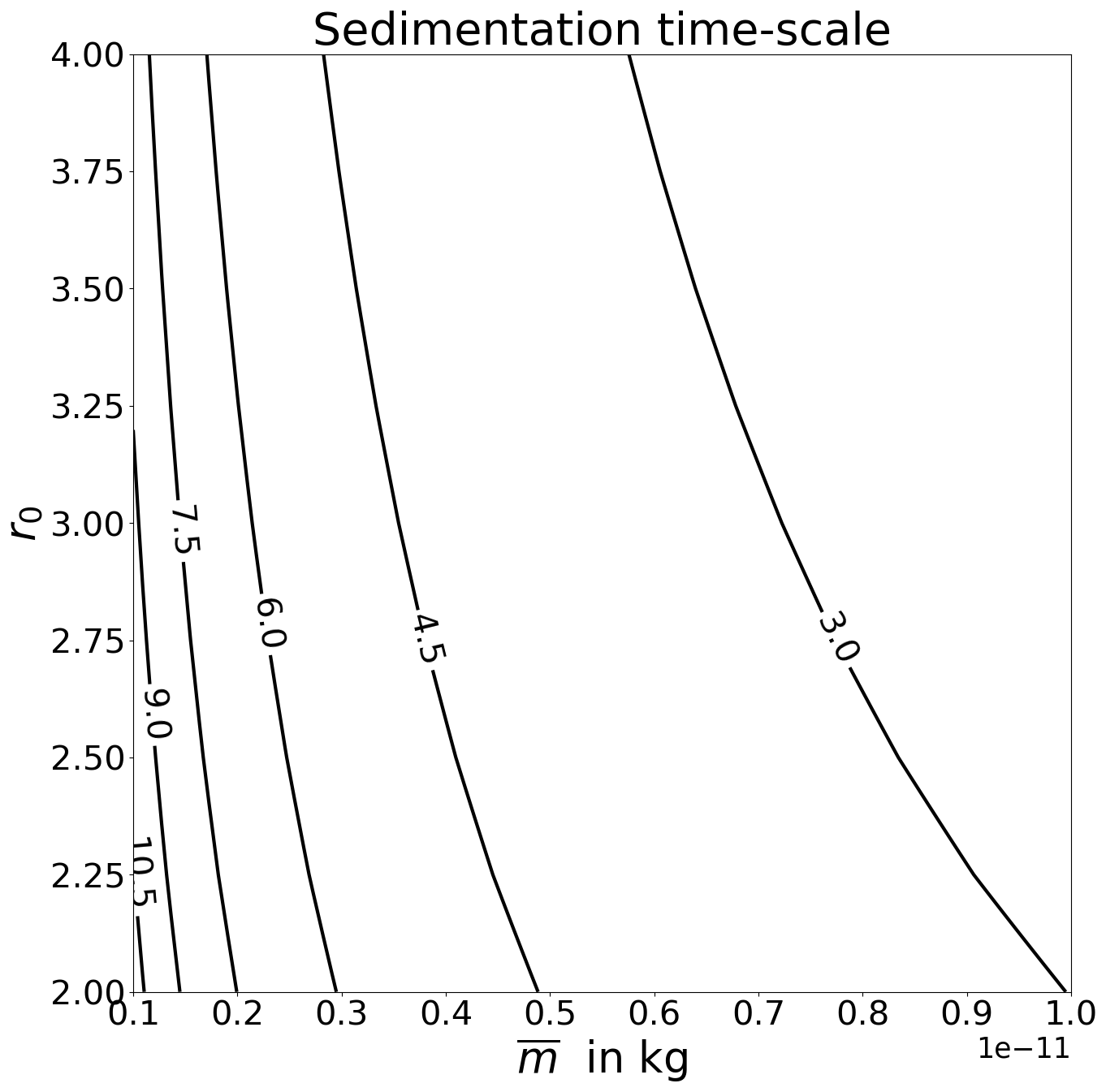
Figure 1 Timescale for sedimentation of ice crystals out of contrails with a 500 m vertical extension H, in hours as a function of mean crystal mass $\stackrel{\mathrm{‾}}{m}$ and mass distribution width parameter r₀. As the timescale is proportional to H, timescales for different values of H can easily be derived from these curves; for instance, a timescale of 6 h for an H = 500 m would reduce to 3 h for H = 250 m.

3.2 Contrail movements relative to ice-supersaturated regions

3.2.1 Timescale for contrails to leave an ISSR with the wind in theory

The following results show that the time span (T) for which an air parcel resides within an ISSR follows a Weibull distribution:

$$\begin{array}{}\text{(4)}& S\left(T\right)=\mathrm{1}-F\left(T\right)=\exp \left[-(T/T_{\mathrm{0}}{)}^k\right].\end{array}$$

Here, S(T) is the survival function and F(T) is the cumulative distribution function of T (see Gierens and Vázquez-Navarro, 2018). For the case of sedimentation, we defined a timescale as the time span during which a fraction of about e⁻¹ of the ice mass is still left in the contrail. To be consistent with that definition, we define the timescale τ_syn for leaving an ISSR as that time, where the survival function reaches the same value: $S\left({\mathit{\tau }}_{\mathrm{syn}}\right)=e^{-\mathrm{1}}$. This time is given by the parameter T₀, independently of the exponent k of the Weibull distribution. Our result is thus

$$\begin{array}{}\text{(5)}& {\mathit{\tau }}_{\mathrm{syn}}=T_{\mathrm{0}}.\end{array}$$

The Weibull fits in the paper yield straight lines of the form

$$\begin{array}{}\text{(6)}& \ln \left\{\ln \left[\mathrm{1}/\left(S\right)\right]\right\}=\mathit{\beta }+k\ln \left(T/T_{\mathrm{u}}\right),\end{array}$$

where β is the intercept, k is the slope and T_u is a unit of time, e.g. 1 s. Solving for the survival function and using Eq. (4) yields

$$\begin{array}{}\text{(7)}& {\mathit{\tau }}_{\mathrm{syn}}=T_{\mathrm{0}}=T_{\mathrm{u}}\exp \left[-(\mathit{\beta }/k)\right].\end{array}$$

A contour plot showing the synoptic timescale as a function of β and k is given in Fig. 2.

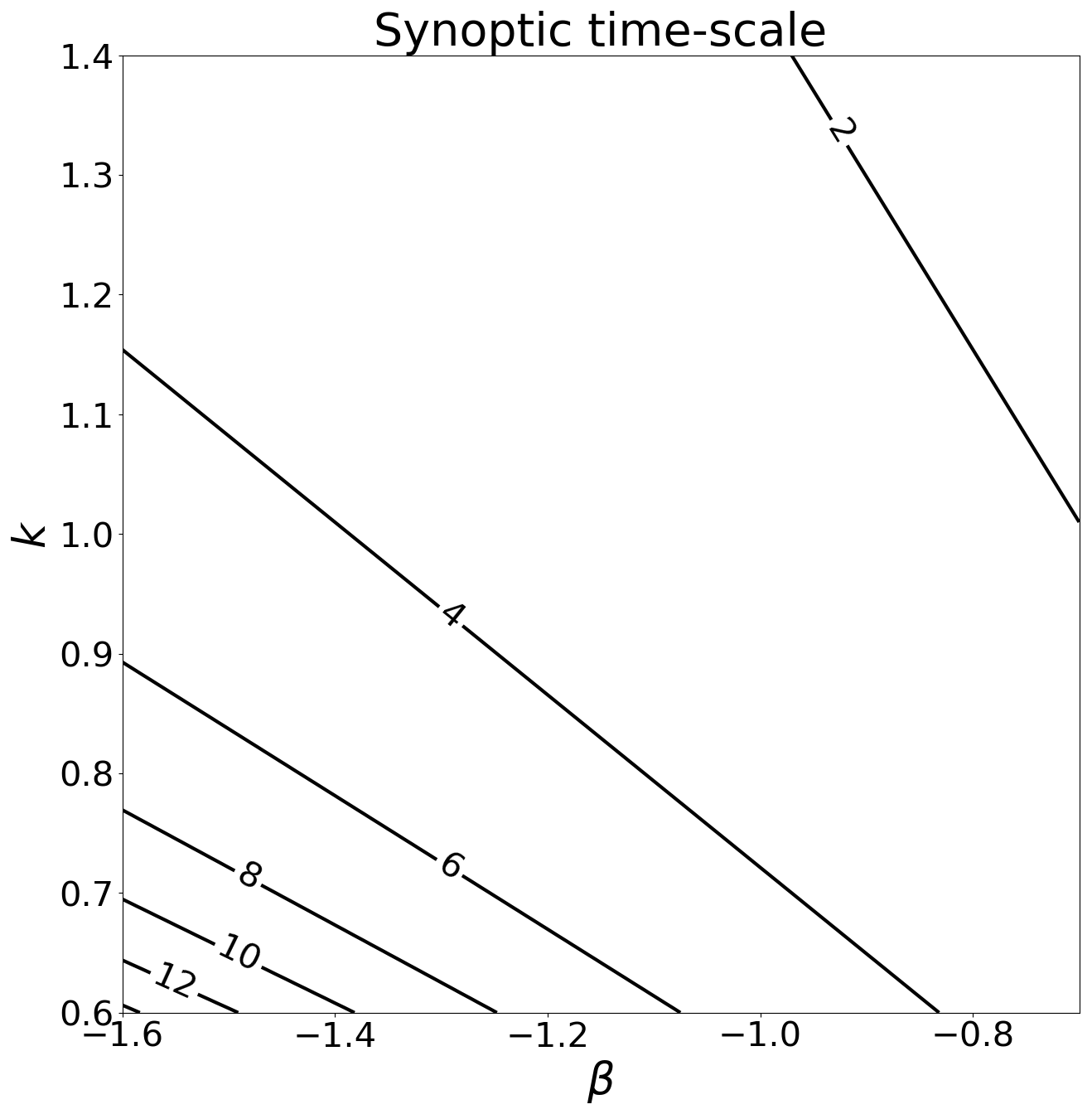
Figure 2 Timescale for contrails to leave an ISSR (in hours). Small values of τ_syn can be reached for small absolute values of β and large values of k and vice versa. Small values of τ_syn indicate that the synoptic pathway of contrail dissolution may dominate.

3.2.2 Trajectory calculations and determination of synoptic timescales

The synoptic timescales are computed statistically. We consider air parcels at grid points with PPC = 1 and determine how long they remain ice-supersaturated during a series of WAWFOR forecast times up to 25 h. To this end, we perform trajectory calculations, which are started 1 h after the initialisation of the forecast. For each subsequent hour, it is tested to confirm whether or not an initially ice-supersaturated air parcel is still supersaturated. For this decision, the RH_i value of the grid point where the air parcels arrive after 1 h (transported by the wind) is used. Air parcels that are still supersaturated are transported further for the next hour; the others are no longer transported. This procedure is repeated until the last forecast step, 24 h after starting time. Initially, and at each subsequent time step, the number of air parcels that are still supersaturated is recorded. These numbers yield the survival function S(t) (i.e. the number of air parcels that are supersaturated at time step t, divided by the number of initially supersaturated air parcels). The statistical analysis of this function provides the desired synoptic timescale.

However, systematic errors due to the 1 h time step cannot be excluded. Air parcels at the edge of an ISSR could leave and re-enter it within 1 h or even re-enter another ISSR that might be nearby or appear as a new ISSR. This can lead to errors, in particular when ISSRs in the forecast have small-scale structures such that their perimeter-to-area ratio is large. The problem should be small for large continuous ISSRs with little small-scale structure (in the forecast).

4 Case studies

In the following, various examples of the movement of areas with PPC = 1 at the forecast initialisation are shown under different weather conditions. The following three dates are selected: 18 April, 1 May and 24 May 2024. First, the synoptic weather situation is briefly described for each day. For this, we show maps of the normalised geopotential height Z^∗; the normalisation procedure is described in Wilhelm et al. (2022). The normalisation of the geopotential has the advantage of spanning a unique range, regardless of the pressure level considered. To this end, each pressure level is assigned a “nominal” geopotential height, and then the actual value of the geopotential height is divided by the nominal value. This results in a small range of values around unity. Furthermore, the maps show where the air moves upward (blue) or downward (red) together with the ISSRs (stippling). Then, a series of plots show both the initial PPC = 1 region (red outline) and the ISSRs 1 or more hours later (blue outline); additionally, the plots show (in green) all grid points where the initially supersaturated air parcels (potential persistent contrails) have been transported to and where they have survived so far. The green area thus diminishes during the plot series. Finally, the survival function is plotted on the so-called Weibull paper – that is, in such a way that a Weibull distribution appears as a straight line, from which we can determine slope and intercept.

In the first two examples, only the start and end times of the ISSR situations are shown. In the last example, some more steps in between are also shown for illustration purposes.

4.1 Case 1: 18 April 2024

The weather situation on 18 April 2024 (12:00 UTC) and in the following hours is characterised by a trough in the upper troposphere that begins over Sweden and extends over Germany and Italy and as far as North Africa. This trough is closely linked to the formation of high- and low-pressure regions on the ground. On the back of the trough, the isohypses run closer together and converge. Due to the greater curvature of the isohypses at the southwestern tip of the trough axis, the wind is slowed down. This leads to the air accumulating in front of the trough axis. In order to balance out the excess mass in front of the trough axis, air masses are transported away. Since the tropopause is soon reached above, the air masses are preferentially transported downwards. This motion increases the air pressure on the ground and a high-pressure region is formed on the back of the trough. On the front side of the trough, the curvature of the isohypses decreases as they diverge. This leads to a lack of mass, which is compensated for by air masses rising from below. This causes the air pressure on the ground to fall, and a low-pressure region is created.

The large-scale sinking of air masses on the back of the trough and the rising in the front of the trough can also be seen in Fig. 3: there, on the back of the trough, mainly red areas (sinking) and, on the front of the trough, mainly blue areas can be seen (rising). Consequently, ice supersaturation occurs on the front side of the trough, in particular at its northeastern edge. It should also be emphasised that ice supersaturation occurs mainly at Z^∗ ≥ 0.98.

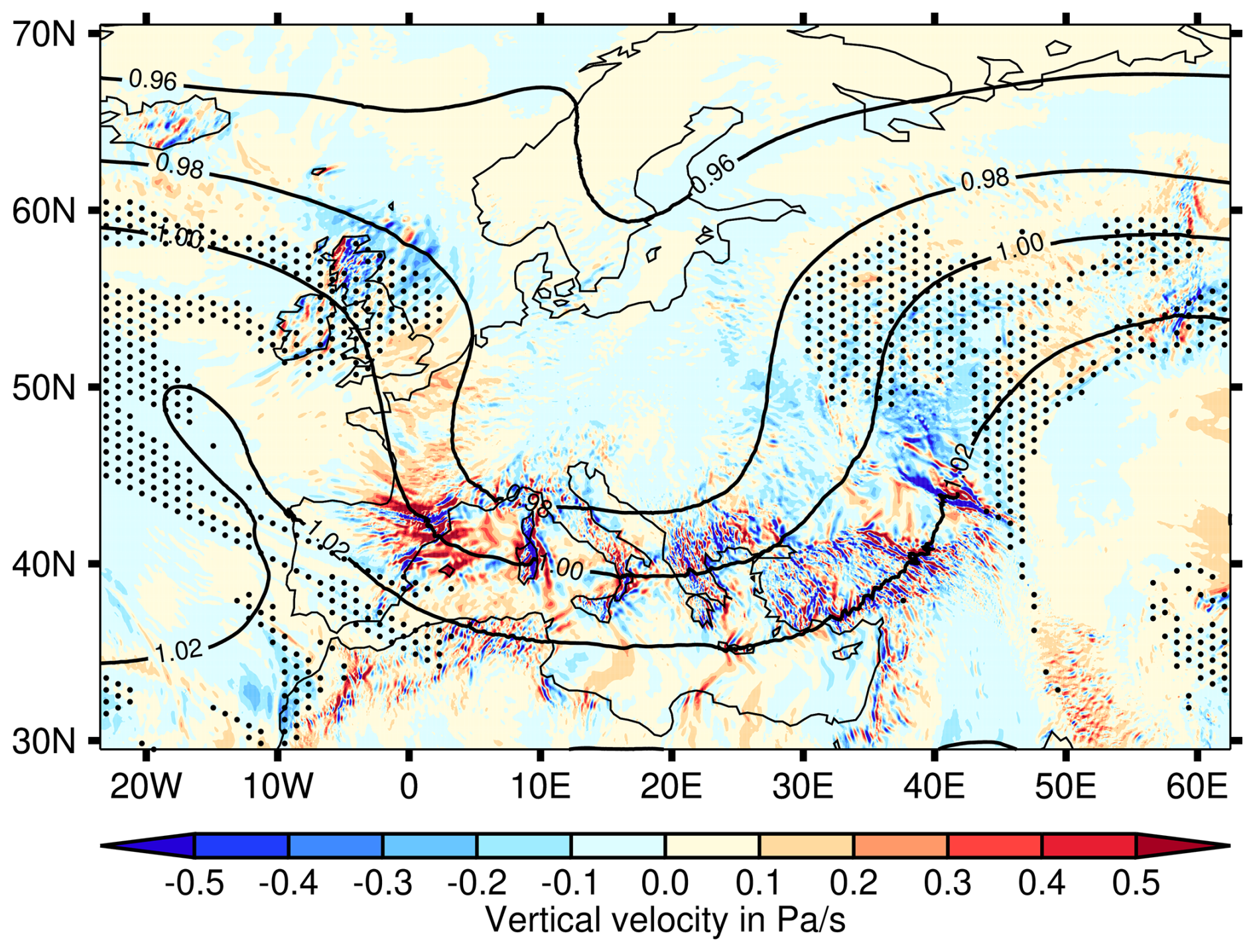
Figure 3 The synoptic situation for 18 April 2024 at 12:00 UTC. Shown are the normalised geopotential height (contours), the vertical velocity (in pressure coordinates) and the ISSRs (stippling) at 250 hPa.

In Fig. 4, the PPC = 1 region at the start time (18 April 2024, from the forecast of 12:00 UTC+1 h) is shown as the red contours in both panels. The blue contours show the ISSRs 1 h later on the left panel and 24 h later on the right panel. The green colour shows the initial PPC = 1 grid points that are still inside the ISSRs – that is, the grid points are all within the blue contours. After 1 h there are still about 75 % of the green points, but 24 h later only very few (< 1 %) green points are still present.

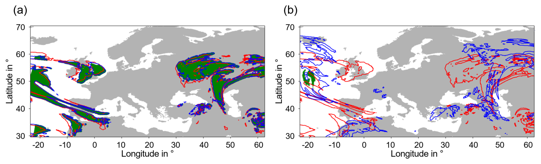
Figure 4 PPC = 1 regions (red contours) at the beginning (18 April 2024, from the forecast of 12:00 UTC+1 h) at 250 hPa in both panels and the ISSRs (blue contours) in the following hour (a) and 24 h after the beginning (b). The green colour shows the initial PPC = 1 grid points that are still inside the ISSRs.

Figure 5 shows the survival function of the number of grid points that were initially within PPC = 1 regions and that stayed continuously within the ISSRs together with the best linear fit on the Weibull paper. The fit can reproduce the curve very well and only deviates slightly towards the end for large values of T, where the statistics get worse because the number of surviving air parcels gets smaller and smaller with increasing T. For this case, we determine a slope of k = 0.9 and an intercept of β = −1.1. According to Fig. 2, this implies a timescale of approximately 4 h.

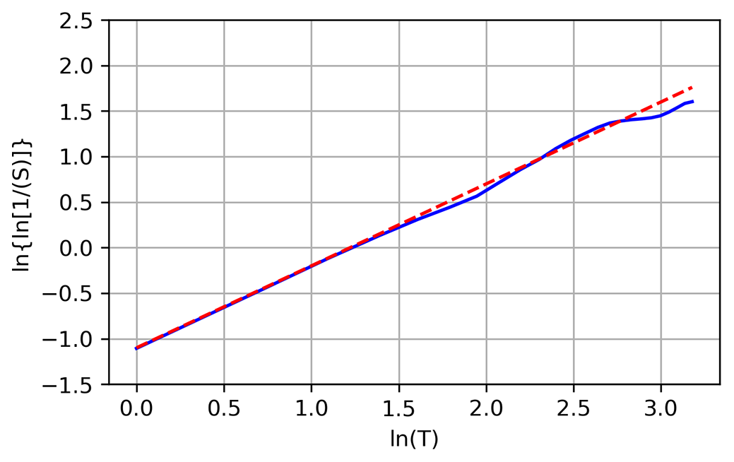
Figure 5 Survival function of the number of grid points that were initially within PPC = 1 region and that survive by always being recorded within an ISSR in the following hours (blue), plotted on Weibull paper together with a linear fit as a dashed line: $g=\mathrm{0.9}\cdot x-\mathrm{1.10}$ (red).

4.2 Case 2: 1 May 2024

The synoptic situation on 1 and 2 May 2024 is primarily determined by the wedge, which stretches from the Mediterranean Sea off the coast of Libya and Egypt across Türkiye, Poland and Scandinavia to the northern coast of the UK (see Fig. 6). Also in this case, ice supersaturation mainly exists for Z^∗ ≥ 0.98 in areas with upward air movement.

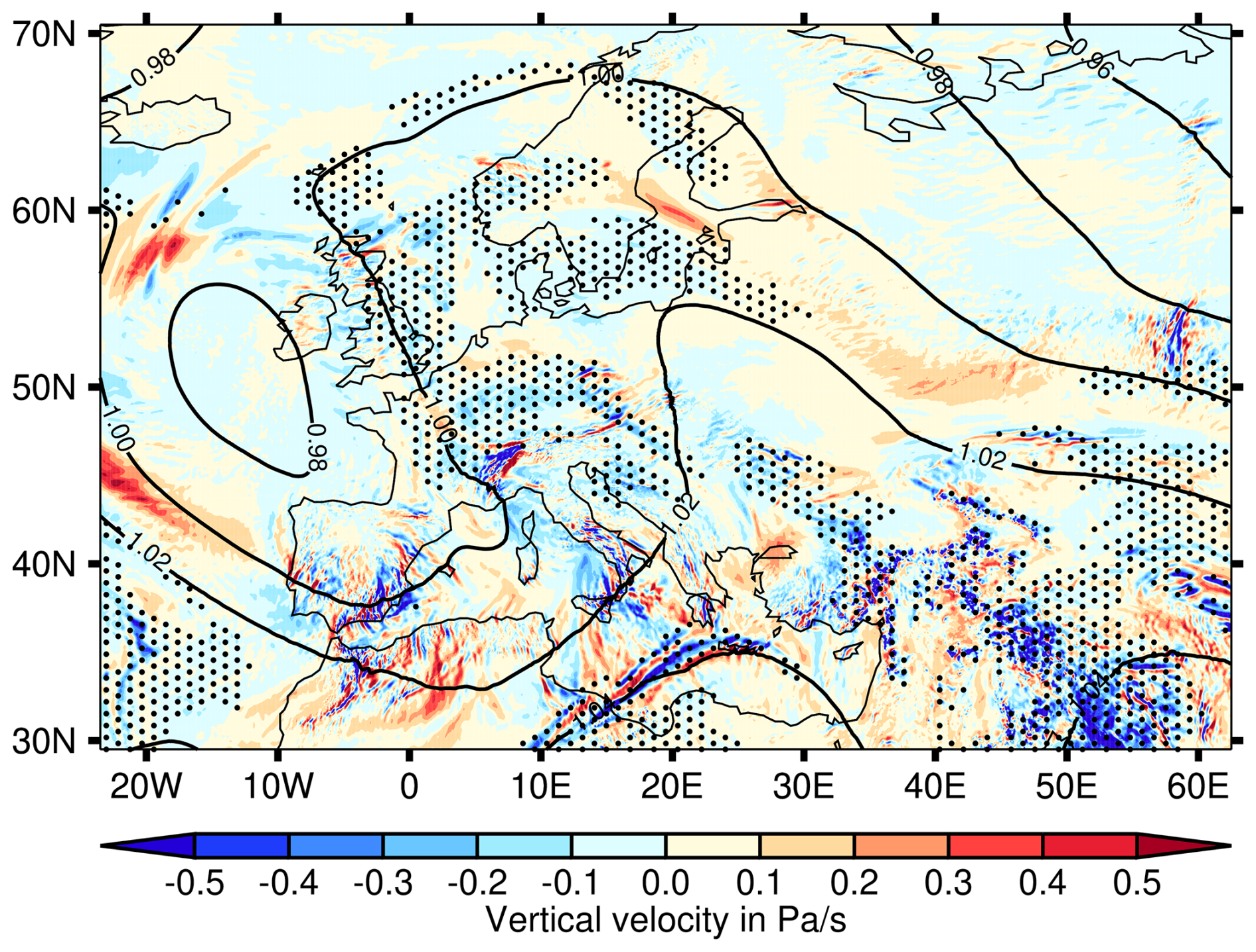
Figure 6 Synoptic situation for 1 May 2024 at 12:00 UTC. Shown are the normalised geopotential height (contours), the vertical velocity (in pressure coordinates) and the ISSRs (stippling) at 250 hPa.

Figure 7 shows the PPC = 1 region at the start time (1 May 2024, from the forecast of 12:00 UTC+1 h) as the red contours in both panels. The blue contours show the ISSRs 1 h later on the left and 24 h later on the right panel. The green colour shows the initial PPC = 1 grid points that are still inside the ISSRs. After 1 h there are still many green points (about 71 % survive) but after 24 h almost all (99.8 %) have vanished.

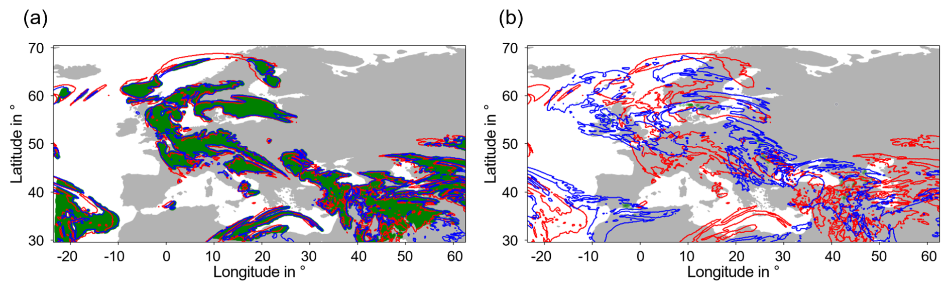
Figure 7 PPC = 1 regions (red contours) at the beginning (1 May 2024 from the forecast of 12:00 UTC+1 h) at 250 hPa in both panels and the ISSRs (blue contours) on the following hour (a) and 24 h after the beginning (b). The green colour shows the initial PPC = 1 grid points that are still inside the ISSRs.

The survival function for this case can be fitted with a Weibull distribution with a slope of k = 0.92 and an intercept of β = −1.09 (see Fig. 8). The synoptic timescale is thus again about 4 h.

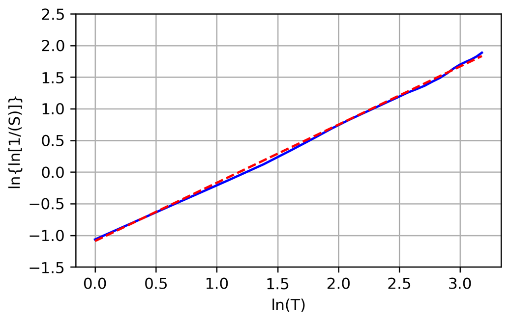
Figure 8 Survival function of the number of grid points that were initially within PPC = 1 regions and that survive by always being recorded within an ISSR in the following hours (blue), plotted on Weibull paper together with a linear fit as a dashed line: $g=\mathrm{0.92}\cdot x-\mathrm{1.09}$ (red).

4.3 Case 3: 24 May 2024

This situation (see Fig. 9) is characterised by high values of the normalised geopotential height throughout the considered region and also large areas with ice supersaturation over Scandinavia, Russia, central Europe, Iran, Libya and Egypt, which occurs mainly in rising air at Z^∗ > 1.0.

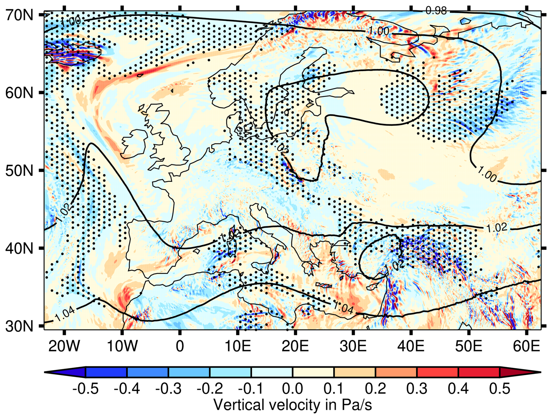
Figure 9 Synoptic situation for 24 May 2024 at 12:00 UTC. Shown are the normalised geopotential height (contours), the vertical velocity (in pressure coordinates) and the ISSRs (stippling) at 250 hPa.

Figure 10 shows the evolution of the surviving initial contrail grid points in more detail – that is, with more intermediate time steps. The PPC = 1 regions at the start time (24 May 2024, from the forecast of 12:00 UTC+1 h) are again shown as the red contours in all panels. The blue contours show the ISSRs 1 h (a), 3 h (b), 5 h (c), 10 h (d), 15 h (e) and 24 h (f) later. The green colour shows as usual the initial PPC = 1 grid points that are still inside the ISSRs at the respective time steps. The number of green points decreases continuously over time. After 1 h, about 76 % of the air parcels are still supersaturated, but after 24 h less than 0.1 % survive.

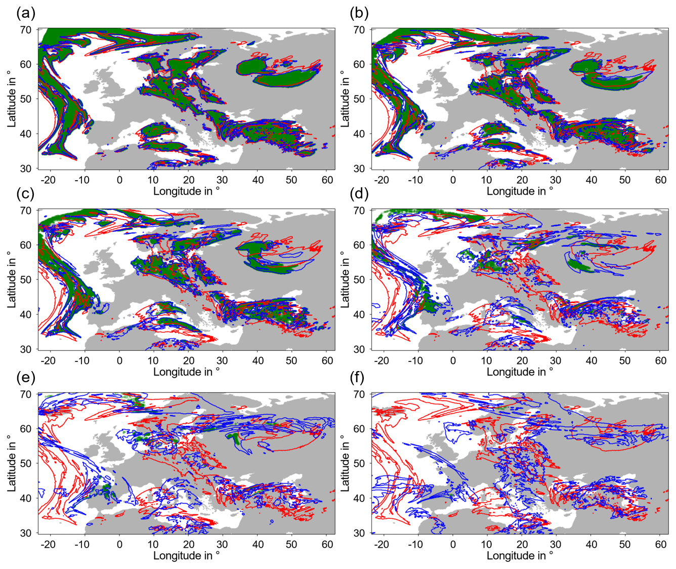
Figure 10 All panels show the PPC = 1 regions at the beginning (24 May 2024 from the forecast of 12:00 UTC+1 h) at 250 hPa as red contours. The six different panels indicate ISSRs from a selection of the following hours in blue (horizontally from top left to bottom right: ISSRs 1 h later at 12:00 UTC+2 h, ISSRs 3 h later, ISSRs 5 h later, ISSRs 10 h later, ISSRs 15 h later and ISSRs 24 h later). Grid points that were within ice supersaturation in every subsequent hour since the beginning are marked in green.

Figure 11 shows the survival function for this case. The best Weibull fit for this case has a slope of k = 1.02 and an intercept of β = −1.30. This is nearly an exponential distribution (which would have k = 1). The corresponding timescale is again about 4 h.

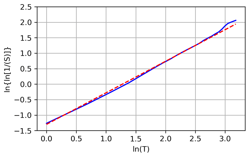
Figure 11 Survival function of the number of grid points that were initially within PPC = 1 regions and that survive by always being recorded within an ISSR in the following hours (blue), plotted on Weibull paper together with a linear fit as a dashed line: $g=\mathrm{1.02}\cdot x-\mathrm{1.30}$ (red).

5 Discussion

5.1 Seasonal and geographical variability

The three case studies have been performed for ISSRs in a certain season (spring 2024) over a certain geographical region (Europe and the western North Atlantic). The resulting synoptic timescales may thus lack generality and may vary if other seasons and other geographical regions are considered. ISSRs may vary in horizontal extension and their own lifetime, due to the prevalent synoptic situations in different parts of the world. Unfortunately, there is not much known about these issues, since ISSRs cannot be observed directly. However, there are at least indirect indications, for instance, the so-called potential contrail coverage (ISSRs where the thermodynamic contrail formation criterion is fulfilled; Sausen et al., 1998) and the path length distribution of aircraft that cross ISSRs (Spichtinger and Leschner, 2016). The potential contrail coverage is larger over the USA and Southeast Asia than it is over Europe and the North Atlantic (Sausen et al., 1998). Path lengths through ISSRs are on average larger in the extratropics than in the tropics (Spichtinger and Leschner, 2016), but the path length distributions overlap substantially. In the extratropics, path lengths are larger in autumn and winter than in spring and summer, whereas in the tropics the seasonal differences are smaller. In any case, due to the strongly skewed path length distributions, the geographical and seasonal differences are much smaller than the standard deviations of the distributions. Variations in potential contrail coverage and path lengths may imply corresponding variations in the synoptic timescales. But the large variability, indicated in the path length distributions, may imply that these variations are statistically insignificant.

5.2 Comparison with results from the literature

The results obtained in our case studies all gave Weibull-type survival functions, with parameters β slightly below −1 and k between 0.9 and about 1. The corresponding synoptic timescales are close to 4 h in all three cases. We can compare these results with results from the literature.

Let us first mention that contrail lifetimes obtained from a study using satellite tracking of contrails (Gierens and Vázquez-Navarro, 2018) gave a mean lifetime of 3.7 h, which is consistent with both the synoptic and the sedimentation timescales derived in this study (although the comparison is a little off since the mean of a Weibull distribution differs from its scale parameter). Unfortunately, the satellite tracking cannot distinguish whether a contrail disappeared due to the sedimentation of its crystals or due to sublimation in dry air, in particular, as the late contrail evolution can often not be observed in satellite images due to vanishing contrast. To determine the mean lifetimes in the satellite study, the authors applied statistical arguments and modelling, based on the Weibull distribution, which provided a good fit with the observed survival function. The parameters in that study led to a quite short timescale of about 0.6 h, a consequence and indication of the fact that only a part of the contrail lifetime can be observed via satellite tracking.

A direct comparison is possible with the results of trajectory calculations presented by Dietz (2012). He uses NWP data from the COSMO model version that was operational in 2012. This was equipped with a 1-moment microphysics scheme. Furthermore, he uses a non-operational version with a 2-moment scheme (Köhler and Seifert, 2015). The resulting survival functions are fitted with Weibull distributions, as in the present study. Additionally, two versions of trajectories are calculated: (1) trajectories from the model data (that is, affected by all processes implemented in the model) and (2) a version where the effects of microphysics are switched off. This means that condensation, sedimentation and precipitation are switched off. This conserves the initial absolute humidity in the idealised simulations (which in reality is reduced by cloud formation) to obtain a “virtual” relative humidity. The following timescales are determined (k values in brackets).

• 1-moment scheme: 3.0 h (k = 0.9);

• 2-moment scheme: 3.8 h (k = 0.75);

• 1-moment scheme, virtual “RH_i”: 4.0 h (k = 0.75);

• 2-moment scheme, virtual “RH_i”: 5.6 h (k = 0.875).

Two observations are immediately possible: first, the 2-moment scheme leads to longer timescales, and, second, the virtual humidity fields have longer timescales than the real humidity fields. This can be explained quite easily. The 2-moment scheme allows higher ice supersaturation to be obtained in the NWP model than the 1-moment scheme. Thus, ISSRs in the 2-moment schemes have on average higher maximum humidities, and it takes longer for them to dry out than for the 1-moment scheme. Switching off microphysics – in particular, switching off the sedimentation of ice crystals – leads again to longer timescales in both model versions. These two timescales are those that are most directly comparable to the ones that we derived here. Indeed, as our trajectories are based on ICON equipped with a 1-moment model, the synoptic timescales are equal: 4 h. We note, however, that our k values are slightly larger than those obtained by Dietz (2012). This difference might result from methodical differences between our study and that of Dietz (for instance, he used three-dimensional trajectories, calculated with a Runge–Kutta method; our approach was simpler, with a two-dimensional Euler forward method).

Numerical simulations of contrails, either with cloud-resolving models (e.g. Unterstrasser and Gierens, 2010a, b; Lewellen, 2014) or with global circulation models (e.g. Bier et al., 2017), provide information on contrail dissolution processes as well. Cloud-resolving simulations usually assume constant synoptic conditions such that contrail dissolution is then only possible via microphysical processes. But it is not only sedimentation that occurs then. Depositional growth of ice crystals reduces the supersaturation in the contrail-containing ISSRs, but it does not lead to subsaturation. Thus, crystal loss in this case is still dominated by sedimentation. In their simulations, Unterstrasser and Gierens (2010a) observe fallstreaks developing after 6500 s (1.8 h), but these consist of only a few large crystals. Most of the contrails cease to grow in mass after 3–4 h, when sedimentation and crystal growth (in a constant supersaturation field) balance out. Without synoptic evolution, the total extinction first grows. Then, after about 3 h, it stagnates or begins to decline, which is due to sedimentation. The authors consider the 3 h an intrinsic timescale for contrails, where “intrinsic” means that it is determined by microphysics rather than synoptic evolution. All the sensitivity studies in Unterstrasser and Gierens (2010b) show the same 3 h intrinsic timescale. Lewellen (2014) often finds contrails with lifetimes exceeding 10 h. This may seem quite high, but it is within the range of the timescales derived here. Synoptic changes that would lead a contrail into subsaturated environments are not simulated, and the thickness of the supersaturated layer is assumed to range from 500 to 1500 m. As the author simulates contrails up to their complete demise, contrail lifetimes can be quite long. For comparison, with a height of 1000 m, the timescales shown in Fig. 1 must be doubled. Since these are e-folding times, the total lifetimes can easily be 2 or 3 times as long. Thus, there is no contradiction between the present and Lewellen's results.

The simulation with a global circulation model that for the first time (to our knowledge) introduced the distinction between the microphysical and the synoptic pathway to contrail dissolution was that of Bier et al. (2017). These authors also mentioned precipitation (the aggregation of ice crystals to snowflakes that fall) and the mixing with ambient natural cirrus (or the replacement of contrail cirrus by natural cirrus) as contrail-terminating processes but with a considerably smaller effect than sedimentation and synoptic drying. In the study, large contrail clusters are formed on several days and their evolution is observed. In the eight considered cases, sedimentation dominates contrail dissolution in three cases and synoptic drying in two cases. The remaining three cases are transition cases (probably cases with τ_sed ≈ τ_syn). Although the lifetimes of a contrail cluster are not simply comparable to the timescales considered here, we can see from their figures that several properties of the clusters change at a high rate during the first few hours, but then, after about 5 to 8 h, further changes are weak. All cases show this behaviour, and this suggests that both timescales should be of the order of 5–8 h, consistent with our results. Bier et al. (2017) also study the effect of a reduction of the initial ice crystal number in the contrails, for example, due to alternative fuels. This leads to larger ice crystal masses and thus, according to Eq. (3), to a shorter sedimentation timescale. Accordingly, all simulations with reduced ice crystal numbers show shorter contrail lifetimes. Interestingly, the contrail lifetimes are also reduced in the dynamically controlled cases. The explanation for this is probably that in the simulations both processes occur simultaneously, and sedimentation is active in dynamically controlled cases as well.

As both processes – sedimentation and synoptic evolution – occur simultaneously in nature, the combined timescale is half the harmonic mean of the two timescales, because

$$\begin{array}{}\text{(8)}& \begin{array}{l}\frac{\mathrm{1}}{\mathit{\tau }}=\frac{\mathrm{1}}{{\mathit{\tau }}_{\mathrm{sed}}}+\frac{\mathrm{1}}{{\mathit{\tau }}_{\mathrm{syn}}};\text{thus}\\ \mathit{\tau }={\displaystyle \frac{{\mathit{\tau }}_{\mathrm{sed}}{\mathit{\tau }}_{\mathrm{syn}}}{{\mathit{\tau }}_{\mathrm{sed}}+{\mathit{\tau }}_{\mathrm{syn}}.}}\end{array}\end{array}$$

Figure 12 The combined timescale of τ_sed and τ_syn in hours, calculated according to Eq. (8).

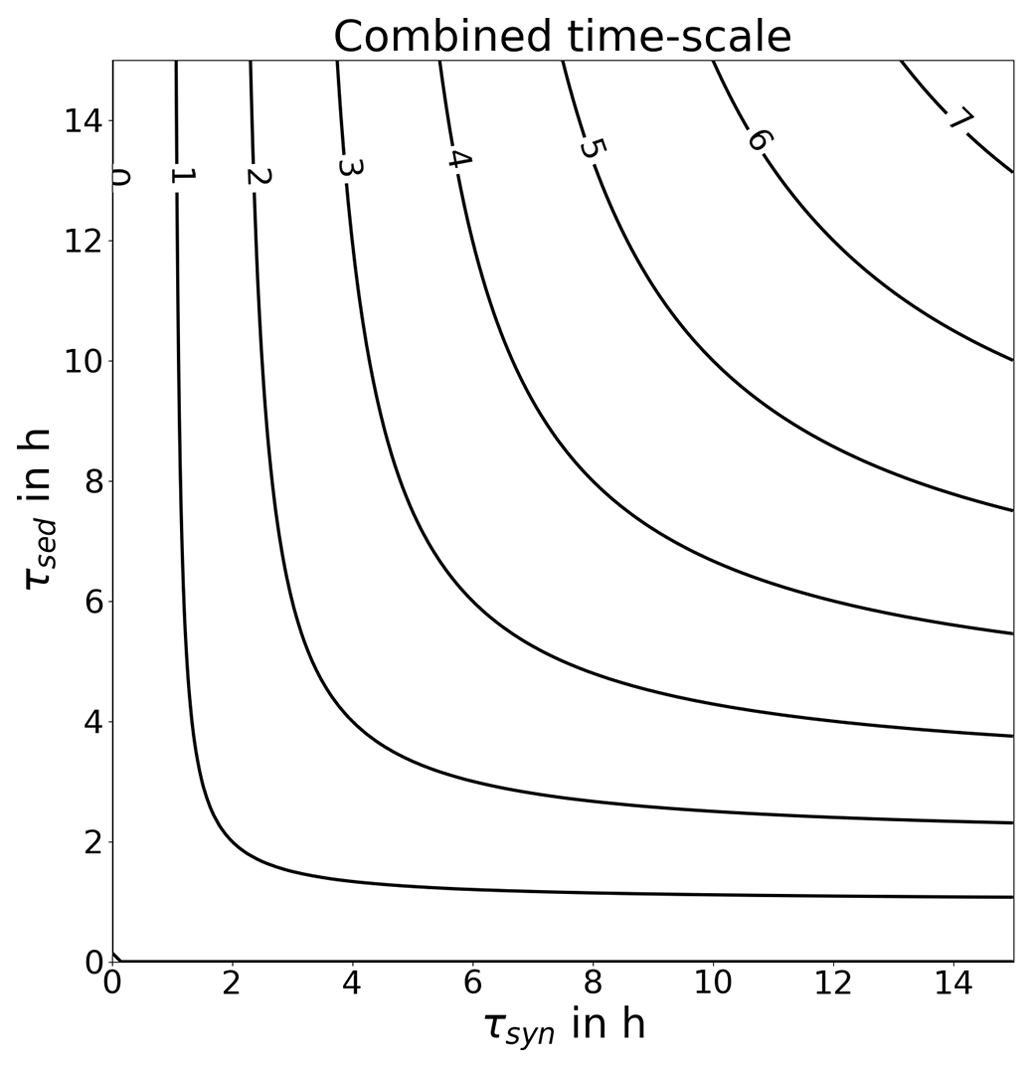
The combined timescale is thus shorter than the two timescales in separation (see Fig. 12). It is also shorter than the smaller one of the two timescales. Even if both timescales were to be 10 h, the combined one is only 5 h, which is plausible, since two processes act simultaneously to dissolve the contrail. This probably explains why the satellite observations give shorter timescales than the cloud-resolving simulations, which typically assume constant synoptic conditions and horizontally periodic boundary conditions.

Furthermore, model simulations allow us to follow a process up to the very end simply by looking at the output values. In contrast, it is difficult in nature to follow a contrail until complete dissolution. This holds for all methods: for satellite imagery, with in situ measurements with research aircraft and with ground observations. Finally, in a model, one has the whole ISSR at hand – that is, one can determine its area, volume, ice, water vapour content, etc. Likewise, if a cloud or contrail is modelled, its properties are in principle completely knowable. This is not possible in nature, neither for ISSRs nor for clouds and contrails. These issues render the comparison of measured and modelled results difficult.

5.3 ISSRs in the synoptic situation

The synoptic weather charts shown to describe the three cases display the normalised geopotential height Z^∗, instead of the geopotential height per se. This quantity has been introduced by Wilhelm et al. (2022) to make variations of this field comparable, i.e. to bring them onto a common scale for different pressure levels. This scale ranges from about 0.9 to about 1.1, independent of pressure in the upper troposphere. Wilhelm et al. (2022) already pointed out that regions where persistent contrails can form are characterised by high values of Z^∗. This finding is corroborated by the current results: in case 1, there are very few (< 10) grid boxes that have ice supersaturation at Z^∗ < 0.98. Otherwise, ice supersaturation occurs exclusively where Z^∗ > 0.98. In cases 2 and 3, there is no ice supersaturation at all where Z^∗ < 0.98. Of course, ISSRs and regions with Z^∗ > 0.98 are not identical. This implies that for contrail avoidance it is still necessary to predict ice supersaturation. The fact that ISSRs are hardly present in regions with Z^∗ < 0.98 renders the prediction work easier. In such regions it is not necessary to think about contrail prevention – they will hardly persist, if they form at all. Calculating Z^∗ from the normal geopotential height involves the call of one simple function, but this very simple step could save a lot of interpretation work later on in the flight planning.

This result could only be obtained by normalising the geopotential. Had we not normalised it, the boundary that corresponds to Z^∗ = 0.98 would appear at different heights at different pressure altitudes and it would be difficult to notice that there is such a boundary at all.

6 Conclusion

Contrails are dissolved mainly by the following processes:

• the sedimentation of the ice crystals into lower levels that are subsaturated,

• the (horizontal) wind blowing the ice crystals out of the parent ISSRs,

• the large-scale subsidence diminishing supersaturation down to subsaturation.

The first of these processes can be characterised by a sedimentation timescale τ_sed, which is proportional to the height of the supersaturated layer and which depends more weakly than linearly on the mean mass of the contrail ice crystals. Typical values are a couple of hours.

The other two processes can together be characterised by a synoptic timescale τ_syn, which does not depend on characteristics of the contrail or its ice crystals but only on the large-scale synoptic situation and, in particular, the relative motion of the parent ISSR and the local wind (see Hofer and Gierens, 2025a). The synoptic timescale is also on the order of a couple of hours. We note, however, that the analysis of the current paper involves only three case studies for ice-supersaturated regions in two spring months over a region in the northern mid-latitudes, mainly Europe and the western North Atlantic. Synoptic situations that are prevalent in spring over this region thus shape the resulting Weibull distributions and, in turn, determine the resulting synoptic timescale. It may well be that these results would be different in other seasons and in other regions of the world where the synoptic circumstances differ from those over the North Atlantic and Europe. As the sizes of ice-supersaturated regions vary seasonally and geographically (Sausen et al., 1998; Spichtinger and Leschner, 2016), the synoptic timescale is expected to vary as well. Whether it varies simply in proportion to the mean size of ISSRs is unknown.

The fact that both timescales are similar may explain why it is unknown whether the microphysical or the synoptic pathway dominates in contrail dissolution. But it can also imply that often both pathways are of similar importance.

As other contrail-removing processes are of minor importance, it is the combination of the two timescales that characterises the lifetime of contrails. This combination is half the harmonic mean of the two timescales in separation, which is always less than the smaller of the two timescales. The timescales in the current paper are defined as e-folding times. Total lifetimes are perhaps 2 or 3 e-folding times.

Cloud-resolving models of contrails usually assume constant synoptic conditions and, applying periodic boundary conditions, effectively assume horizontally and infinitely extended ISSRs. Thus, the synoptic timescale is effectively infinite. Contrail lifetimes in these models are often quite long (> 10 h). In contrast, contrail simulations in global circulation models where both pathways are effective yield shorter contrail lifetimes (say, about 5–8 h). Both pathways are also effective in nature. Contrail-tracking studies using satellite imagery thus find short lifetimes of the order of 4 h.

The sedimentation timescale of a contrail can be diminished if alternative fuels with reduced soot emission (by number) are applied, as long as the reduction does not lead to the so-called soot-poor regime (that is, where the soot emission index would fall below 10¹³⁻¹⁴ soot particles per kg of fuel; see Kärcher and Yu, 2009). Less soot implies fewer but larger ice crystals (i.e. with a higher mean mass). Thus, the microphysical timescale can be reduced by technical means, whereas the synoptic timescale is given by the weather situation. For an effective means of contrail mitigation, the resulting sedimentation timescale must be smaller than the synoptic timescale. In order to determine this in the flight planning phase, trajectory calculations would be necessary. There are already services for contrail avoidance in place or under development (e.g. Engberg et al., 2025), which use trajectory calculations to compute the advection of a contrail with the wind. If they represent ice crystal sedimentation in a reliable way, the preflight estimation of the two timescales should in principle be possible.

Finally, a side result of this study is that contrails will hardly persist in regions where the normalised geopotential height, as defined by Wilhelm et al. (2022), is less than 0.98. This simple boundary can easily be calculated for the upper troposphere, and we strongly recommend that aviation weather forecasts use normalised geopotential height on their synoptic charts because this allows flight planners to immediately see where contrail prevention actions are not necessary.

Note, however, that Wilhelm et al. (2022) derived their statistics from flight data obtained in the northern mid-latitudes. It is not known whether this simple result can be generalised to, for instance, more tropical regions. In any event, most air traffic currently occurs in the northern mid-latitudes and, for this region, the recipe should be applicable.