Global patterns and trends in ground-level ozone chemical formation regimes from 1996 to 2022

Ground-level ozone (O₃) formation in urban areas is nonlinearly dependent on the relative availability of its precursors: oxides of nitrogen (NO_x) and volatile organic compounds (VOCs). To mitigate O₃ pollution, a crucial question is to identify the O₃ formation regime (NO_x-limited or VOC-limited). Here, we leverage ground-based O₃ observations alongside space-based observations of O₃ precursors, namely, nitrogen dioxide (NO₂) and formaldehyde (HCHO), to study the long-term shifts in O₃ chemical regimes across global source regions. We first derive the regime threshold values for the satellite-derived $\mathrm{HCHO}/{\mathrm{NO}}_{\mathrm{2}}$ ratio by examining its relationship with the O₃ weekend effect. We find that a regime transition from VOC-limited to NO_x-limited occurs around 3.1 [2.7–3.4] for $\mathrm{HCHO}/{\mathrm{NO}}_{\mathrm{2}}$ with slight regional variations. By integrating data from four satellite instruments, including Global Ozone Monitoring Experiment (GOME), SCanning Imaging Absorption spectroMeter for Atmospheric CHartographY (SCIAMACHY), Ozone Monitoring Instrument (OMI) and TROPOspheric Monitoring Instrument (TROPOMI), we built a 27-year (1996–2022) satellite $\mathrm{HCHO}/{\mathrm{NO}}_{\mathrm{2}}$ record from which we assess the long-term trends in O₃ production regimes. A discernible global trend towards NO_x-limited regimes is evident, particularly in developed regions such as North America, Europe, and Japan, with emerging trends in developing countries like China and India over the past 2 decades. This shift is supported by both increasing $\mathrm{HCHO}/{\mathrm{NO}}_{\mathrm{2}}$ ratios and a diminishing O₃ weekend effect. Yet, urban areas still hover in the VOC-limited and transitional regime on the basis of annual averages. Our findings stress the importance of adaptive emission control strategies to mitigate O₃ pollution.

1 Introduction

Ozone (O₃) near the surface is an air pollutant with profound implications for human health and Earth's ecological system (Chiu et al., 2023; Nuvolone et al., 2018; Mills et al., 2016; Felzer et al., 2007). It is known to cause respiratory and cardiovascular diseases (World Health Organization, 2021). Chronic exposure to O₃ has been linked to an estimated 1.04 to 1.23 million premature mortalities globally in 2010, primarily due to respiratory ailments (Malley et al., 2017), and this issue of O₃-related deaths has the potential to worsen despite the improvement in other air pollutants like fine particulate matter (Wang et al., 2021). In addition to its harmful effects on human health, O₃ poses a threat to other species by inducing DNA damage in animals and affecting crop productivity and yield through disrupting the plant microflora (Manisalidis et al., 2020).

Ground-level O₃ is a secondary air pollutant formed through photochemical reactions between oxides of nitrogen (NO_x) and volatile organic compounds (VOCs). At the ground level, O₃ formation is dominated with the NO_x-limited regime globally, especially in rural or sparsely populated regions (Monks et al., 2015). In areas with high NO_x emissions and relatively low VOC emissions, such as urban and metropolitan centers, O₃ formation can become NO_x-saturated or, in other words, VOC-limited. Freshly emitted NO, particularly from vehicular traffic, can locally deplete O₃ by reacting with it (Solberg et al., 2005), thereby curtailing O₃ accumulation in the immediate vicinity. Consequently, lower O₃ concentrations are typically observed in urban areas (Simon et al., 2024; Paoletti et al., 2014). Over the past several decades, the evolution of global O₃ formation has been shaped by a complex interplay of socio-economic factors, including varying industrial activities and population movements, as well as environmental policies and changing climate (Zhang et al., 2019; Pfister et al., 2014). The combined effects of these factors are highly intricate. For instance, sustained declines in NO_x and VOC emissions have led to reductions in peak O₃ concentrations in many developed countries, but mitigating O₃ exposure at the urban scale is still challenging owing to the nonlinearity of O₃–NO_x–VOC chemistry (Simon et al., 2016). Therefore, understanding the O₃ production regimes transition and its drivers are essential for devising effective mitigation strategies.

O₃ sensitivity cannot be directly observed, which is often diagnosed through analyzing the relationship between observed O₃ and its precursors, or using measurements of indicator species such as NO_y, formaldehyde (HCHO), reactive nitrogen (NO_y), hydrogen peroxide (H₂O₂) and nitric acid (HNO₃) (Sillman, 2012, 1999; Tonnesen and Dennis, 2000). However, ground-based measurements of these indicators are often limited, making satellite remote sensing a vital alternative for expanding the monitoring of these atmospheric species. Satellites provide retrievals of two key species: HCHO (Fu et al., 2007; Palmer et al., 2003), which is nearly proportional to the summed rate of VOC reactions with hydroxyl radicals (OH) and thus serves as an effective VOC tracer (Sillman, 2012). Nitrogen dioxide (NO₂) is prevalent in the boundary layer atmosphere and represents the majority of NO_x (Duncan et al., 2010). The ratio of HCHO to NO₂ ($\mathrm{HCHO}/{\mathrm{NO}}_{\mathrm{2}}$) has been used to infer O₃–NO_x–VOC sensitivity (Jin et al., 2020, 2017; Jin and Holloway, 2015; Choi et al., 2012; Duncan et al., 2010; Martin et al., 2004). An important issue to use satellite $\mathrm{HCHO}/{\mathrm{NO}}_{\mathrm{2}}$ is to determine the threshold values separating the NO_x-limited and VOC-limited regimes. Martin et al. (2004) and Duncan et al. (2010) use 1 and 2 as regime threshold values, but follow-up studies show that the regime threshold values are uncertain (Jin et al., 2017; Souri et al., 2023; Wang et al., 2021; Schroeder et al., 2017).

Over the past 2 decades, the global distributions of HCHO and NO₂ concentrations have been shaped by diverse emission reduction policies, resulting in distinct regional changes. In terms of NO₂, many anthropogenic regions have witnessed nonlinear shifts or reversal years in NO₂ pollutant levels (Georgoulias et al., 2019), in developed regions, such as the US and European countries, substantial reductions in NO_x emissions have been achieved, largely due to stringent national regulations (Department for Environment, Food & Rural Affairs, UK, 2024; Toro et al., 2021; Krotkov et al., 2016; Russell et al., 2012), whereas in developing regions, NO_x emission reductions have normally lagged behind. According to Zhao et al. (2013), there was a surge in NO_x emissions in China until around 2010, after which a decline was observed. This decrease has been linked to technological advancements and the implementation of emission control measures in key industries (Sun et al., 2018). Given the diverse trends of O₃ precursor emissions, less is known about how the O₃ production regime has changed over the past few decades because of the emission changes. Here, we aim to identify the long-term trends in satellite $\mathrm{HCHO}/{\mathrm{NO}}_{\mathrm{2}}$ and the reversal years in different regions, which could signal a change in the direction of O₃ chemical regime changes.

Another widely used method to characterize O₃ formation regimes is through comparing the weekend versus weekday difference (WE-WD) in O₃ and its precursors. Under high NO_x mixing ratios, O₃ production rates paradoxically increase as NO_x concentration falls; conversely, in scenarios with low NO_x mixing ratios, O₃ production rates decline. In most urban areas, characterized by high NO_x levels, O₃ concentrations frequently display a significant rise on weekends relative to weekdays. Reasons for this “O₃ weekend effect” can be multifaceted and region-specific, involving reduced NO_x concentrations altering VOC ratios, timing shifts in NO_x emissions, increased VOC and NO_x emissions on weekend nights, and enhanced sunlight due to lower particulate matter emissions. This distinctive WE-WD O₃ pattern has been observed globally; first documented in New York City, US (Cleveland et al., 1974); and subsequently reported in various regions, including Europe (Sicard et al., 2020; Adame et al., 2014), East Asia – Tokyo, Japan (Sadanaga et al., 2012), Pearl River Delta (PRD) (Zou et al., 2019), North China Plain (NCP) (Wang et al., 2014), Yangtze River Delta (YRD) (Tang et al., 2008) and Taiwan (Tsai, 2005); North America – Mexico (Stephens et al., 2008) and the entire US (Jaffe et al., 2022; Atkinsonpalombo et al., 2006); and major cities in Latin America – Santiago, Chile (Seguel et al., 2012), and Rio de Janeiro, Brazil (Martins et al., 2015). The varying O₃ weekend effect provides an opportunity to evaluate the chemical regimes of O₃ (Simon et al., 2024; Jin et al., 2020).

In this study, we aim to elucidate the long-term shifts in O₃ chemical regimes on a global scale using the two indicators: satellite-derived $\mathrm{HCHO}/{\mathrm{NO}}_{\mathrm{2}}$ ratios and ground-based observation of O₃ weekend effect. In Sect. 3.1, we examine the surface WE-WD O₃ concentration as a function of the tropospheric column $\mathrm{HCHO}/{\mathrm{NO}}_{\mathrm{2}}$ ratio to identify the thresholds distinguishing different O₃ regimes. In Sect. 3.2, we analyze the long-term trend of satellite-based $\mathrm{HCHO}/{\mathrm{NO}}_{\mathrm{2}}$ and identify the trend reversals. These two steps set the stage for evaluating the long-term evolution of O₃ production regime. In Sect. 3.3, we analyze whether the satellite-derived $\mathrm{HCHO}/{\mathrm{NO}}_{\mathrm{2}}$ ratio trends align with the long-term patterns of the O₃ weekend effect, offering dual evidence on the evolving O₃ chemical regimes. The HCHO and NO₂ retrievals integrate 27-year (1996–2022) data from four satellite instruments: GOME/ERS-2, SCIAMACHY/ENVISAT, OMI/Aura and TROPOMI/Sentinel-5P. In Sect. 3.4, we further investigate the global spatiotemporal evolution of O₃ chemical regimes, focusing on their transition status and potential transition years. By examining the long-term trends of $\mathrm{HCHO}/{\mathrm{NO}}_{\mathrm{2}}$ ratios and applying region-specific thresholds, we categorize the evolution of O₃ regimes into four main types: constant regimes, constant quasi regimes, single-shift regimes and multiple-shift regimes. Overall, our goal is to provide insights into O₃ regime variations across regions and decades, which could inform air quality management strategies about the effective strategies to mitigate O₃ pollution.

2 Data and methods

2.1 Harmonized satellite retrievals of O₃ precursors

We combine satellite retrievals of tropospheric NO₂ and HCHO vertical columns from four different satellite instruments, including Global Ozone Monitoring Experiment (GOME), SCanning Imaging Absorption spectroMeter for Atmospheric CHartographY (SCIAMACHY), Ozone Monitoring Instrument (OMI) and TROPOspheric Monitoring Instrument (TROPOMI). We use satellite-based products developed under the Quality Assurance for Essential Climate Variables (QA4ECV) project, which retrieves NO₂ and HCHO consistently using the same model simulations from TM5-MP as an a priori profile that features consistent meteorology, emissions and chemical mechanisms (Boersma et al., 2018, 2017a, b, c; De Smedt et al., 2017, 2018; Williams et al., 2017). The nadir resolution is 320 km×40 km for GOME, 60 km×30 km for SCIAMACHY, 24 km×13 km for OMI and 5.5 km×3.5 km for TROPOMI. The overpass time is around 10:00 LT for SCIAMACHY and GOME, ∼ 13:30 LT for OMI and TROPOMI.

To investigate the long-term changes in $\mathrm{HCHO}/{\mathrm{NO}}_{\mathrm{2}}$, we construct annual average tropospheric NO₂ and HCHO vertical column density (VCD) data from the GOME (1996–2001), SCIAMACHY (2002–2003), OMI (2004–2020) and TROPOMI (2020–2022) datasets. GOME, SCIAMACHY and TROPOMI data are harmonized with reference to OMI data with a resolution of 0.25°×0.25°. The retrieval and harmonization scheme are described in Jin et al. (2020). Briefly, we use OMI as a reference to adjust GOME and SCIAMACHY columns as OMI has the finest spatial resolution and the overpass time of interest where it captures the most active O₃ formation chemistry. For NO₂, the difference among satellite instruments is decomposed into two components: (1) difference due to resolution and (2) difference due to overpass time. The difference due to resolution is adjusted by comparing the differences in re-gridding Level-2 OMI NO₂ to a fine-resolution (0.25°×0.25°) grid versus a coarse-resolution (2°×0.5°, resolution closer to that of GOME) grid. The difference in overpass time is derived from the mean difference between OMI and SCIAMACHY during overlapping years (2004–2012) at a coarse resolution (2°×0.5°). For HCHO, as the spatial variations in HCHO are mostly regional, the harmonization only accounts for the difference caused by overpass time (Jin et al., 2020). We grid all Level-2 satellite HCHO products to 0.25°×0.25° and adjust GOME and SCIAMACHY HCHO columns by adding the mean difference between SCIAMACHY and OMI during the overlapping period. We do not adjust for the difference between OMI and TROPOMI as their overpass time is close.

2.2 Ground-based O₃ observations

For O₃ data, we rely on the TOAR-II database (Schultz et al., 2017a, b). Initiated by the Global Atmospheric Chemistry Project (GACP), TOAR has been developing a cutting-edge database that provides hourly surface O₃ concentrations on a global scale since 1970 (Schultz et al., 2017a), serving as an unparalleled resource for examining temporal trends in surface O₃ levels (Sicard et al., 2020). Notably, the observation record period varies across monitoring stations, with earlier data in the US, Europe and Japan dating back to the 1970s–1980s and later in regions such as South Korea and Latin America from 1995 to 2005. For China, South Africa, Southwest Asia and densely populated Australian areas, records typically begin around 2015. To ensure rigorous study standards, we selected over 8700 stations with at least 3 consecutive years of data for our global analysis. Figure 1 illustrates the distribution of TOAR sites and main regions we focus on.

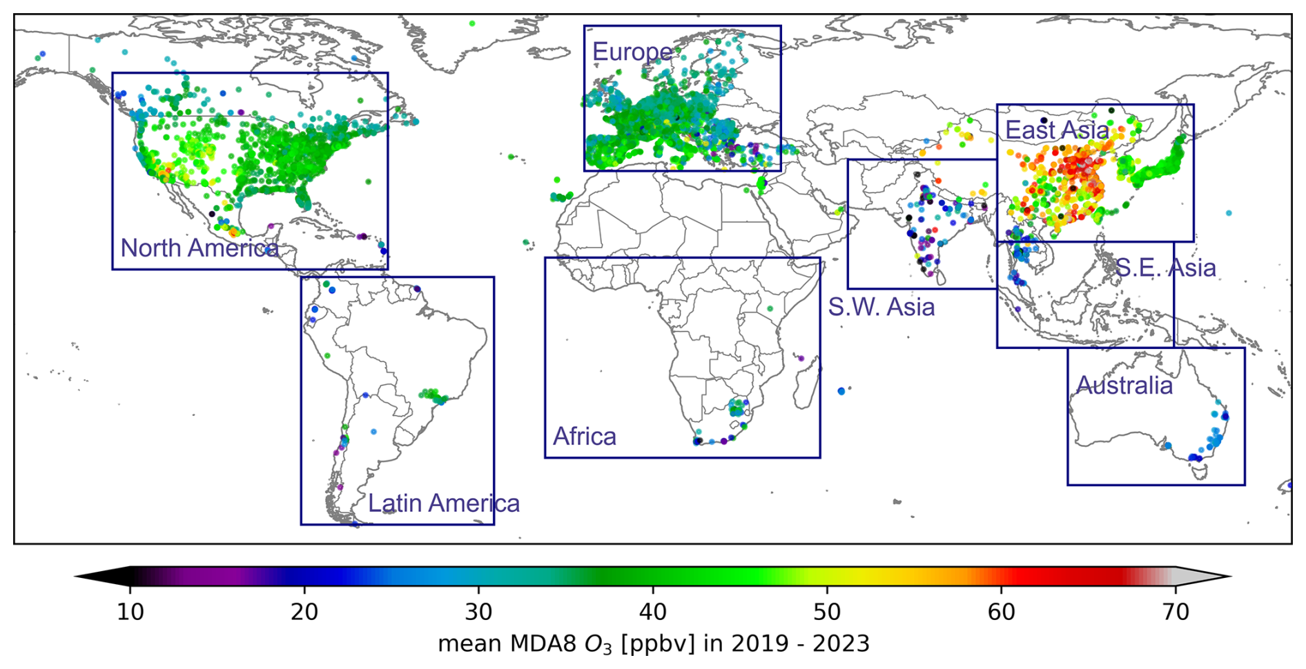
Figure 1 Global distribution of O₃ (unit: ppbv) in the past 5 years (2019–2023). Data are sourced from the TOAR database.

2.3 Ground-based WE-WD O₃ and the connections with satellite $\mathrm{HCHO}/{\mathrm{NO}}_{\mathrm{2}}$

The WE-WD O₃ difference reflects the sensitivity of O₃ to emission reduction in NO_x on weekends, which is effectively the derivative of O₃ with respect to NO_x, and the transitioning point at which O₃ weekend effect crosses zero represents the transitioning point at which O₃ sensitivity to NO_x emission changes signs, which often corresponds to peak O₃ production. In this study, WE-WD O₃ difference is quantified using a standardized protocol: Sundays are designated as weekends, while Tuesdays–Thursdays are designated as weekdays, excluding Mondays and Fridays to minimize transitional effects from adjacent days. For each site and weekly interval throughout the observation period, we calculate the mean differences in WE-WD O₃. To calculate long-term trends of WE-WD O₃ in Sect. 3.3, all sites within the region are included. Given the global scope of this analysis and the inherent complexity in defining distinct O₃ seasons across various regions, we utilize all-year data without seasonal selection. Using the t test at each site to ascertain the statistical significance of WE-WD difference (p value<0.05). Statistically significant WE-WD differences are identified at each site, and trends were evaluated using 5-year rolling intervals to dampen interannual meteorological variability (Pierce et al., 2010).

To build the relationship between the observed O₃ weekend effect and satellite $\mathrm{HCHO}/{\mathrm{NO}}_{\mathrm{2}}$ (Sect. 3.1), we mainly use OMI retrievals of HCHO and NO₂. OMI is selected as the primary satellite data source due to its unique combination of long-term continuity (2004–2020) and optimal afternoon overpass time. The early-afternoon measurement period (13:00–14:00 LT) coincides with peak photochemical activity when O₃ production is the most active, boundary layer heights are maximized, and solar zenith angles are minimized – all critical factors for obtaining high-quality retrievals of tropospheric HCHO and NO₂ columns (Jin et al., 2017; Jin and Holloway, 2015). We derive threshold values for the $\mathrm{HCHO}/{\mathrm{NO}}_{\mathrm{2}}$ ratio that delineate O₃ formation regimes by correlating the WE–WD differences in O₃ with $\mathrm{HCHO}/{\mathrm{NO}}_{\mathrm{2}}$ using linear regression. The regime threshold corresponds to the intercept (zero-crossing point) of the regression line, where the sign of WE–WD O₃ changes. To establish the relationship between $\mathrm{HCHO}/{\mathrm{NO}}_{\mathrm{2}}$ ratios and WE-WD O₃, we extract the nearest gridded daily OMI data (0.125°×0.125°) corresponding to the ground-based O₃ monitoring stations. To ensure precise spatiotemporal matching, we pair the satellite overpass observations with surface measurements by averaging hourly O₃ concentrations at 13:00 and 14:00 LT (corresponding to OMI's overpass window).

2.4 Long-term trend reversal of annual $\mathrm{HCHO}/{\mathrm{NO}}_{\mathrm{2}}$ ratio

As most regions show bi-directional trends of O₃ precursors, we hypothesize that a reversal of trend in $\mathrm{HCHO}/{\mathrm{NO}}_{\mathrm{2}}$ can be found during our study period. To identify trend reversal years for the $\mathrm{HCHO}/{\mathrm{NO}}_{\mathrm{2}}$ ratio at each grid point, we adopt the method Georgoulias et al. (2019) used in the analysis of satellite-derived NO₂ trend reversals, originally adapted by Cermak et al. (2010) for studying solar radiation and global brightening trends. The approach is briefly described as follows.

Firstly, for each grid point and for each year t, a point score S(t) is calculated to quantify the potential for a trend reversal:

$$\begin{array}{}\text{(1)}& S\left(t\right)={\displaystyle \frac{min\left(p\left(B_{\mathrm{1}}\right),p\left(B_r\right)\right)}{\text{abs}(B_l-B_r)\times {\mathit{\sigma }}_{B_{l+r}}}}.\end{array}$$

Here, B₁, B_r and B_1+r represent the trends calculated over 5-year periods to the left, [t−4, t]; right, [t, t+4]; and spanning the year, [t−4, t+4], respectively. The 5-year interval is chosen to reduce the impact of interannual meteorology variability. p(B₁) and p(B_r) are the probabilities (p values) of the trend B being statistically insignificant, while ${\mathit{\sigma }}_{B_{l+r}}$ signifies the error in trend fitting. The p value of the hypothesis test, with the null hypothesis being a zero slope is calculated using a Wald test with a t distribution.

The time series data for each grid and period are fitted to a linear model:

$$\begin{array}{}\text{(2)}& Y_t=A+B{X}_t+N_t,\end{array}$$

where Y_t is the annual-mean value for year t, X_t is time variable representing the year, A is the annual mean of the first year, B is the estimated slope of trend line, and N_t represents the residual or the discrepancy between the fitted and the observed value.

A year is identified as a trend reversal year if it exhibits the lowest S(t) value, an opposite sign between B₁ and B_r ($B_{\mathrm{1}}\times B_r<\mathrm{0}$), and significant trend starts and ends (both p(B₁) and p(B_r)<0.05). Selecting the year with the lowest S(t) ensures a maximal difference in trend slope ($max\mathrm{|}{B}_l-B_r\mathrm{|}$) on either side of the year, with the fitting error in the trend at this juncture, ${\mathit{\sigma }}_{B_{l+r}}$, being as pronounced as possible. This method is estimated to be capable of identifying reversal years with a very limited error of 0.5 %–1 % and standard deviation between 2 % and 5 % (Cermak et al., 2010). The trend calculation, based on data spanning 5 years before and after each year, helps to mitigate the impact of short-term extremes in pollutant concentrations, such as the dramatic decrease in emissions during the 2020 COVID-19 pandemic. This approach allows us to identify regions with long-term changes in trends.

3 Results and discussions

3.1 Identification of region-specific regime thresholds for satellite-based $\mathrm{HCHO}/{\mathrm{NO}}_{\mathrm{2}}$

O₃ formation exhibits complex nonlinear dependence on NO_x and VOC concentrations. During weekends, urban NO_x emissions typically decline (Fig. S1 in the Supplement) due to reduced transportation and industrial activity, leading to distinct O₃ response patterns: in VOC-limited regimes, NO_x reductions cause weekend O₃ increases (WE-WD O₃>0), while NO_x-limited regimes show weekend O₃ decreases (WE-WD O₃<0). The transition between these regimes occurs at a theoretical threshold, which we identify as the $\mathrm{HCHO}/{\mathrm{NO}}_{\mathrm{2}}$ ratio where WE-WD O₃=0. To demonstrate our approach, we selected nine representative urban stations with long-term (>10-year) records, as shown in Fig. 2. These sites were chosen ensuring a balanced global representation while factoring in regional site density (three European, two North American, two Asian, one Australian and one Latin American). Our analysis of monthly WE-WD O₃ differences and $\mathrm{HCHO}/{\mathrm{NO}}_{\mathrm{2}}$ ratios reveals strong negative correlations (fitting line in Fig. 2), consistent with photochemical theory – higher NO_x availability enhances weekend O₃ increases. Assuming WE-WD O₃ differences are primarily NO_x-driven, the $\mathrm{HCHO}/{\mathrm{NO}}_{\mathrm{2}}$ value at the WE-WD O₃=0 crossing can be considered the site-specific thresholds separating VOC-limited and NO_x-limited regimes (red triangle in Fig. 2b1).

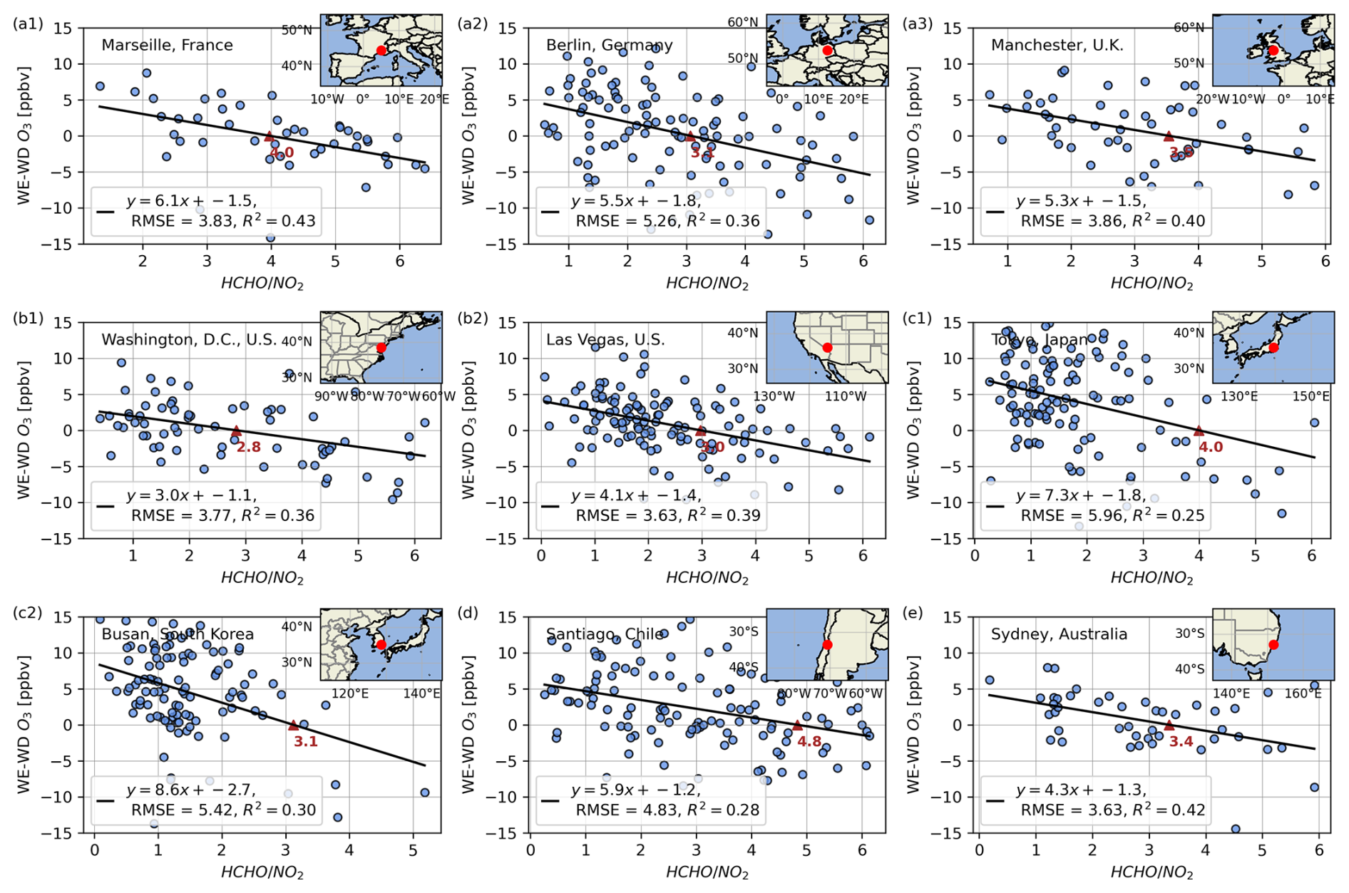
Figure 2 Scatter plots of the monthly average satellite-derived $\mathrm{HCHO}/{\mathrm{NO}}_{\mathrm{2}}$ ratio versus the WE-WD O₃ concentration in nine representative cities. Black line: the fitted linear regression line, red triangles: inflection points where the regression line intersects the WE-WD O₃=0 baseline.

Building upon this qualitative approach, we systematically quantify O₃ sensitivity thresholds across the global monitoring network (Fig. 3). Our analysis of all qualified monitoring sites (R²>0.2) reveals that the probability density distribution of transition thresholds across global stations peaks at $\mathrm{HCHO}/{\mathrm{NO}}_{\mathrm{2}}=\mathrm{3.1}$. The transitional range between VOC-limited and NO_x-limited regimes is quantified using the top 10 % frequency interval ([2.7–3.4] for global sites). The observed spatial patterns may reflect regional disparities in emission profiles and chemical regimes (Lu and Chang, 1998). Longer-regulated regions with balanced emission reductions (e.g., Europe) systematically exhibit higher thresholds than rapidly developing areas where NO_x remains dominant (e.g., East Asia). In East Asia (all sites: 2.8 [2.5–3.2]), extremely low values are observed over the NCP at 2.0 [1.8–2.2], while Japan shows the highest threshold range of 3.8 [3.4–4.2]. Europe shows the highest continental-scale $\mathrm{HCHO}/{\mathrm{NO}}_{\mathrm{2}}$ threshold among all regions studied (all sites: 3.5 [3.2–3.9]). However, significant country-level variations exist, ranging from the lowest values in the UK (2.7 [2.4–3.0]) to the highest in Austria (3.9 [3.6–4.3]). North America also exhibits notable subregional variability in $\mathrm{HCHO}/{\mathrm{NO}}_{\mathrm{2}}$ thresholds (all sites: 3.0 [2.6–3.3]), ranging from elevated values in California (4.0 [3.6–4.4]) to lower thresholds along the Lower Mississippi Valley (LMV) region (2.9 [2.6–3.1]). This pattern aligns with findings from Jin et al. (2020) employing alternative methodologies. Residual discrepancies in absolute threshold values may arise from temporal shifts in emission trends, such as increasing $\mathrm{HCHO}/{\mathrm{NO}}_{\mathrm{2}}$ ratios in recent decades. Regions with limited observational coverage (effective sites <150) still yield meaningful but less constrained distributions, ranging from Europe-like values in Australia (3.4 [3.0–3.7]) to lower thresholds in South Africa (2.7 [2.3–3.2]). Emission heterogeneity and monitoring density may further modulate the interval widths: regions with uneven source distributions or sparse networks likely display broader transition ranges (e.g., Africa, span 0.9: 2.3–3.2) compared to well-monitored regions (e.g., Europe, span 0.7: 3.2–3.9). Other regions – including Southwest Asia (3.1 [2.8–3.3]) and Latin America (3.1 [2.8–3.4]) – cluster near the global mean, suggesting intermediate photochemical regimes.

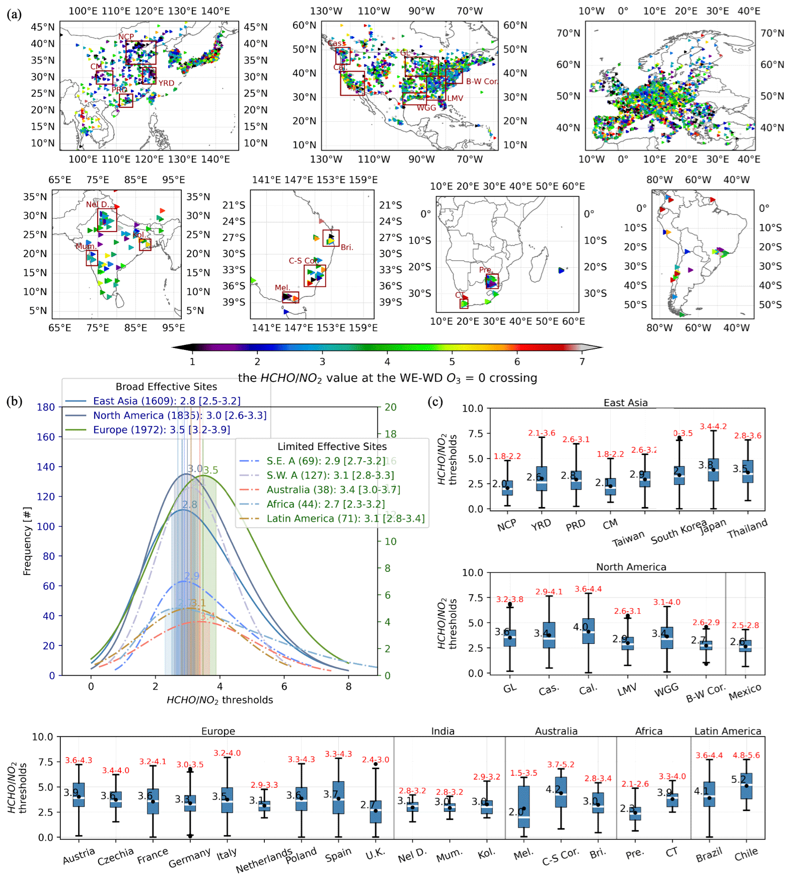
Figure 3 (a) Global map of key $\mathrm{HCHO}/{\mathrm{NO}}_{\mathrm{2}}$ values indicating O₃ regime transition. Red rectangles highlight major economic regions: North China Plain (NCP), Yangtze River Delta (YRD), Pearl River Delta (PRD), and Chongqing Municipality (CM) in China; Great Lakes region (GL), Cascadia region (Gas.), California (Cal.), Lower Mississippi Valley region (LMV), West Gulf Coast (WGG), and Boston–Washington Corridor (BW Cor.) in the US; New Delhi (Nel D.), Mumbai (Mum.), and Kolkata (Kol.) in India; Melbourne (Mel.), Canberra–Sydney Corridor (C–S Cor.), and Brisbane (Bri.) in Australia; and Pretoria (Pre.) and Cape Town (CT) in South Africa. (b) Frequency distribution of $\mathrm{HCHO}/{\mathrm{NO}}_{\mathrm{2}}$ thresholds across regions (R²>0.2). Solid lines denote continents with >1500 valid sites; dashed lines represent regions with <150 sites. (c) Box plots of transition thresholds in economically advanced regions (marked in a). Black numbers: peak $\mathrm{HCHO}/{\mathrm{NO}}_{\mathrm{2}}$ frequencies ($\stackrel{\mathrm{̃}}{x}$), red range: top 10 % frequency interval defining the transitional range [x_lower–x_upper].

The variations in the regime threshold values of $\mathrm{HCHO}/{\mathrm{NO}}_{\mathrm{2}}$ are likely caused by several factors. First, here we use tropospheric column $\mathrm{HCHO}/{\mathrm{NO}}_{\mathrm{2}}$ to represent the near-surface O₃ chemistry, which is affected by the relationships between column and surface HCHO and NO₂ (Jin et al., 2017). The column-to-surface relationship is determined by the boundary layer height and the vertical profiles of HCHO and NO₂, which should vary spatially (Adams et al., 2023; Zhang et al., 2016b). Second, HCHO is used as an indicator of VOCs, but the yield of HCHO from oxidation of VOCs varies with different species (Shen et al., 2019; Chan Miller et al., 2016; Zhu et al., 2014). Regions dominated by biogenic VOC emissions, such as the southeast US and tropical regions, generally have larger HCHO yield (Wells et al., 2020; Palmer et al., 2007, 2006). Third, the local chemical environmental may also differ spatially. For example, the lower thresholds in China are consistent with elevated regional NO_x levels (Jamali et al., 2020) and enhanced secondary aerosol formation in this region, which may promote radical loss (Li et al., 2019; Liu et al., 2012). Here, we use statistical methods to derive the regime thresholds. Further attribution of the spatial variations is beyond the scope of this study, which warrants further investigation.

It should be noted that these calculations do not account for the effects of short-term synoptic processes on temperature and the conditions affecting O₃ transport and diffusion. The regime thresholds have uncertainties, and previous studies have typically assumed a range for regime threshold values (Jin et al., 2020, 2017; Sillman, 1999). This implies that the critical values identified in this study should not be considered definitive indicators that guarantee a regime shift. Nonetheless, this method remains valuable for leveraging large-scale satellite data to track the global progression of O₃ regimes, especially in regions and periods where in situ O₃ data are limited. We will further explore this using the statistically derived threshold in Sect. 3.3.

3.2 Long-term trends in satellite-based $\mathrm{HCHO}/{\mathrm{NO}}_{\mathrm{2}}$

3.2.1 Spatial patterns and linear trends

Given the critical role of satellite-based $\mathrm{HCHO}/{\mathrm{NO}}_{\mathrm{2}}$ in diagnosing O₃ chemical regimes, we first investigate its global distribution (Fig. 4) and long-term trends from 1996 to 2022 across anthropogenic regions (Fig. 5). Multi-year-averaged $\mathrm{HCHO}/{\mathrm{NO}}_{\mathrm{2}}$ ratios identify highly VOC-limited regimes in densely populated urban clusters worldwide, including China's most developed regions (NCP, YRD, and PRD), the Seoul–Incheon metropolitan area in South Korea, the Greater Tokyo region in Japan, the Los Angeles region in the US, the Belgium–Netherlands–eastern UK region in Europe and the Johannesburg area in South Africa. More extensive areas exhibit moderate VOC sensitivity ($\mathrm{1}<\mathrm{HCHO}/{\mathrm{NO}}_{\mathrm{2}}<\mathrm{2}$), covering eastern China; the eastern US; central-western Europe (particularly western Germany, northern France and northern Italy); India's Delhi–Mumbai industrial corridor; Australia's coastal urban centers; and major Latin American metropolitan areas, including Rio de Janeiro, Santiago and Buenos Aires.

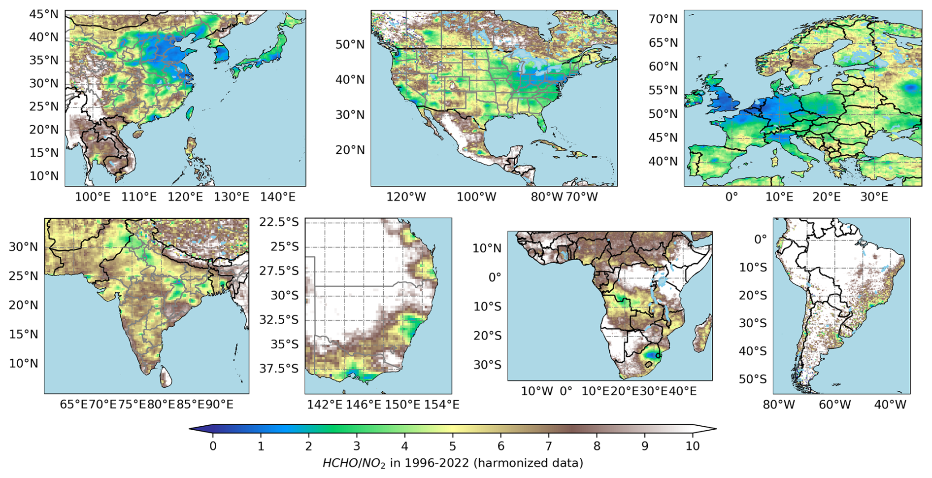
Figure 4 Tropospheric $\mathrm{HCHO}/{\mathrm{NO}}_{\mathrm{2}}$ ratio patterns using the self-consistent GOME, SCIAMACHY, OMI and TROPOMI datasets for the combined period from 1996–2022.

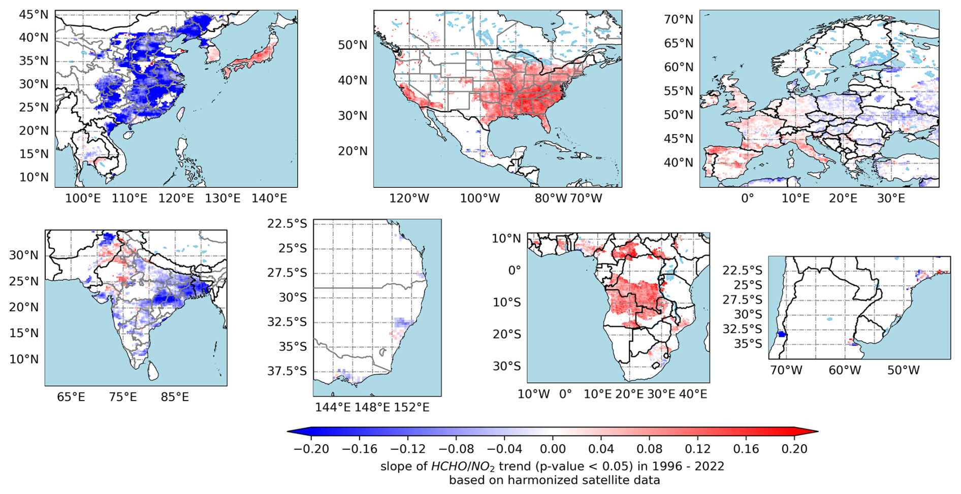
Figure 5 Satellite-based linear trends of tropospheric $\mathrm{HCHO}/{\mathrm{NO}}_{\mathrm{2}}$ ratios (1996–2022) for grids with a mean NO₂ $\text{VCD}>\mathrm{1.5}\times {\mathrm{10}}^{\mathrm{15}}$ (molecules cm⁻²) and statistically significant trends at the 95 % confidence level.

These spatial patterns correlate strongly with NO₂ hotspots (Fig. S2a), reflecting the localized nature of NO_x emissions compared to the more uniform distribution of VOCs (Fig. S2b). NO_x emissions, primarily linked to population density and economic activities, predominantly originate from high-temperature combustion processes involving nitrogen and oxygen, such as industrial emissions and vehicle exhaust (Liu et al., 2016). With its short lifetime of a few hours to a day, the distribution of NO₂ reflects hotspots of power generation and fossil fuel consumption (Jamali et al., 2020). In contrast, HCHO, an intermediate regime in the degradation of various VOCs (De Smedt et al., 2015), exhibits a more uniform distribution due to the widespread biogenic sources of VOCs. This contrast underscores NO_x as the dominant driver of spatial variability in $\mathrm{HCHO}/{\mathrm{NO}}_{\mathrm{2}}$ ratios.

Our analysis of tropospheric $\mathrm{HCHO}/{\mathrm{NO}}_{\mathrm{2}}$ ratio trends reveals significant spatial heterogeneity across global anthropogenic regions (Fig. 5). Focusing on areas with mean tropospheric NO₂ columns exceeding 1.5×10¹⁵ molecules cm⁻² and statistically significant trends (p<0.05), we observe distinct patterns between developed and developing economies. Developed regions, particularly Japan and the US (eastern seaboard and California region), show strong positive trends averaging 0.11 ± 0.05 yr⁻¹, likely reflecting the success of long-term air quality policies in reducing NO_x emissions. Similarly, Taiwan and South Korea exhibit weak positive trends (0.04 ± 0.02 yr⁻¹). In contrast, rapidly developing regions display marked negative trends, with central-eastern China and India showing significant declines (−0.12 ± 0.05 yr⁻¹), including localized minima of −0.18 yr⁻¹ in China's YRD and −0.13 yr⁻¹ in Kolkata region. Similar negative trends are observed in Chile (−0.14 ± 0.02 yr⁻¹), while Australia's southeastern coastal cities show weaker decreases (−0.05 ± 0.03 yr⁻¹). European trends present moderate but complex spatial variability, with urban clusters in western Europe showing slight increases (0.08 ± 0.04 yr⁻¹) and eastern European regions experiencing decreases ($<-\mathrm{0.04}$ yr⁻¹).

The observed trends mirror the global redistribution of O₃ precursors since 1980, where developed nations achieved emission reductions while developing Asia – particularly Southeast, East and South Asia – experienced dramatic increases (Zhang et al., 2016a). Specifically, Europe and North America achieved >60 % NO_x reductions between 1990 and 2022 through stringent air quality policies, while Asia experienced an 86 % increase during the same period, with India's emissions nearly tripling to 9.4 million t by 2022 (https://www.statista.com/, last access: May 2025, noted as Statista data from here on). Although VOC reductions in developed regions (e.g., −46 % in the US since 1990 to 2023, Statista data) would theoretically drive $\mathrm{HCHO}/{\mathrm{NO}}_{\mathrm{2}}$ ratios downward, the observed trends are primarily governed by NO_x dynamics, as evidenced by the stronger correlation between NO₂ and $\mathrm{HCHO}/{\mathrm{NO}}_{\mathrm{2}}$ trends compared to HCHO alone (Fig. S3). Local-scale variations in either VOCs or NO_x may account for regional deviations from these general patterns. Japan represents a unique case in East Asia, showing robust linear growth in $\mathrm{HCHO}/{\mathrm{NO}}_{\mathrm{2}}$ ratios resulting from its early and rigorous regulatory framework targeting both mobile and stationary sources. The country's vehicle emission controls, initiated in 1966 (initially CO-focused), evolved through progressive NO_x standards for light-duty vehicles (1973), stricter gasoline/diesel limits (1989) and world-leading regulations by 2003 (NO_x regulations surpassing contemporaneous US and European standards) (https://www.env.go.jp/air/, last access: May 2025). Parallel industrial policies have revised stationary source NO_x limits four times since 1973. These measures drove a 33.7 % reduction in national NO_x emissions from 2005 to 2014 (1.93 to 1.28 million t; Statista data), positioning Japan's emissions at merely 5.8 % of China's regional total (0.68 vs. 11.76 Tg N yr⁻¹; Han et al., 2020). Satellite data corroborate a 27-year decline in tropospheric NO₂ columns.

Over the African continent, almost no change is detected, with one notable exception – the Congo Basin. This finding aligns with previous satellite observations showing no significant trends in either NO₂ (Hilboll et al., 2013) or HCHO (De Smedt et al., 2015) over most of Africa. However, existing studies have not sufficiently explained the continental disparity between Africa's overall trend stability and the Congo Basin's unique behavior. The Congo Basin presents a particularly intriguing case, exhibiting an anomalously strong negative $\mathrm{HCHO}/{\mathrm{NO}}_{\mathrm{2}}$ trend (Fig. 5) and complex identified reversals (Fig. 6). This region's distinct atmospheric chemistry likely stems from its status as one of the world's most active biomass-burning hotspots, where competing environmental factors may drive the observed anomalies: a global reduction in burned area including Africa (1998–2015; Andela et al., 2017) versus persistent localized fire activity from slash-and-burn agriculture (Tyukavina et al., 2018). These fires complicate the trends of HCHO and NO₂ due to both smoke aerosol interference with satellite retrievals and transient spikes during extreme events (Jin et al., 2023). Consequently, standard trend analysis cannot reliably resolve emission signals in such fire-prone areas, necessitating specialized methodologies beyond this study's scope.

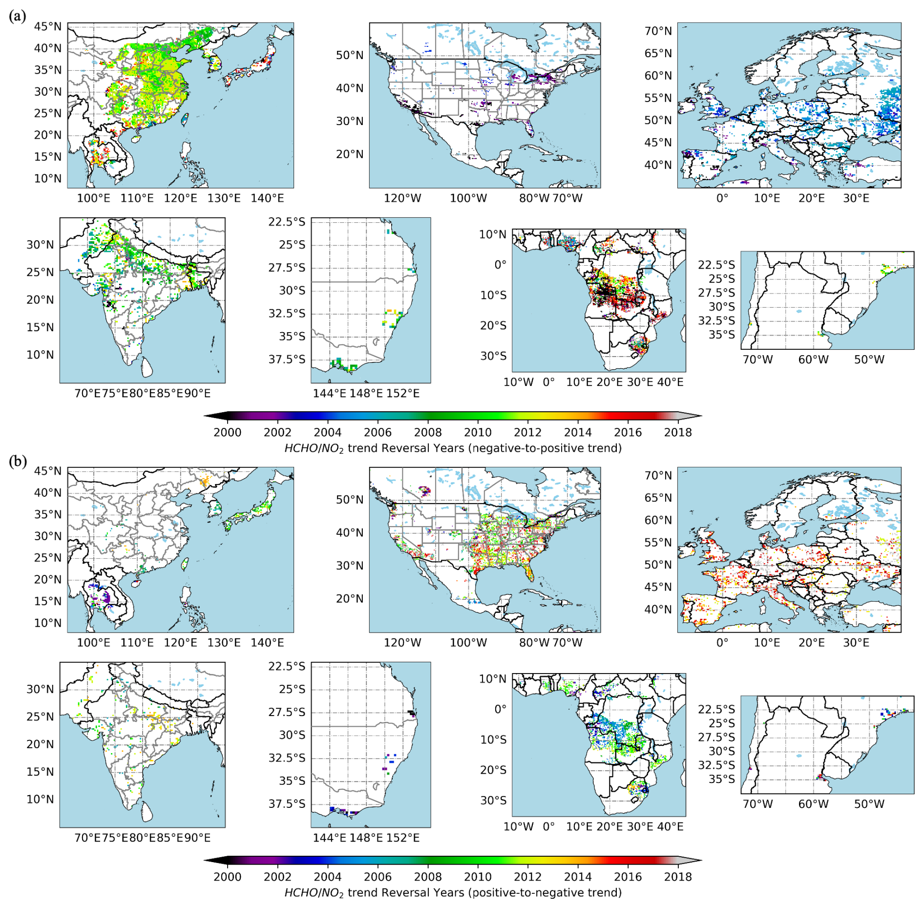
Figure 6 Persistent trend reversals of tropospheric $\mathrm{HCHO}/{\mathrm{NO}}_{\mathrm{2}}$ ratio (a) from negative to positive and (b) from positive to negative. Only grid cells with a with long-term mean NO₂ columns greater than 1.5×10¹⁵ molecules cm⁻² and statistically significant trends with p value<0.05 for the period before and after the year of reversals are shown.

While linear regression effectively captures dominant trends, important nonlinearities emerge in regions undergoing rapid trend transitions. For instance, China's NCP region initially showed steep ratio declines during industrialization followed by stabilization after the implementation of stringent emission controls post-2012 (van der A et al., 2017). Such nonlinear behavior, where rapid industrialization drives initial NO_x surges followed by policy-driven reductions, creates trend reversals that simple linear models cannot resolve. Thus, areas with nonsignificant linear trends in Fig. 5 may conceal abrupt turning points rather than being truly trendless, emphasizing the need for complementary nonlinear analyses.

3.2.2 Drivers of $\mathrm{HCHO}/{\mathrm{NO}}_{\mathrm{2}}$ trend and trend reversals

Next, we assess whether trend reversals exist in $\mathrm{HCHO}/{\mathrm{NO}}_{\mathrm{2}}$ time series. Figure 6 presents our estimated years of persistent reversal occurrence, considering only grid cells with statistically significant trends (p value<0.05) for both pre- and post-reversal periods. Figure 6a shows the regions where we find trend changes from negative to positive, and Fig. 6b shows the regions where the trend transitioned from positive to negative. While some locations experienced multiple reversals, we focus on the most significant transition at each grid point.

The most striking reversals occur in Asia, where East China and parts of India show clear negative-to-positive trend shifts around 2011. In China, this reversal directly corresponds to stringent NO_x controls implemented, including power plant retrofits and upgraded vehicle standards (van der A et al., 2017; Krotkov et al., 2016). This policy-driven transition is clearly reflected in the satellite record, where the inflection point in $\mathrm{HCHO}/{\mathrm{NO}}_{\mathrm{2}}$ ratios aligns closely with the peak and subsequent decline in NO₂ columns (Figs. S3a and S4b). During 1996–2011, NO₂ levels in the NCP region surged 8-fold, far outpacing HCHO increases (1.5 times; Fig. S3a). After 2011, industrial VOC emissions rose by 20.46 % from 2011–2017 (11 122.7×10³ to 13 397.9×10³ t yr⁻¹; Liu et al., 2021), amplifying the post-2011 ratio recovery.

India presents a contrasting case, with more localized and less sustained reversals. While major cities like Delhi and Mumbai saw NO₂ concentrations rise 1.5–2 times during 1996–2022 (tracking 15.6 % average annual gross domestic product growth, GDP, after 2002, https://data.worldbank.org, last access: May 2025), only temporary slowdowns occurred during economic dips (e.g., 2011–2013). During this period, HCHO levels showed only modest growth (1.2 times). The temporary GDP slowdown (1.09 % growth during 2011–2013) seems to correlate with localized NO₂ ratio slowdowns or declines post-2011, though these were neither sustained nor widespread. This pattern reflects fundamental challenges in pollution governance in India – despite establishing early regulatory frameworks like the 1981 Air (Prevention and Control of Pollution) Act and the 2019 National Clean Air Programme (NCAP), implementation has remained weak (Ganguly et al., 2020), somewhat reflect an insufficient policy prioritization of environmental protection.

Developed regions exhibit normally linear dominance with subtle shifts but distinct multi-phase patterns. In the US, initial localized positive trends emerged in the early 2000s. These transitions – from flat or weakly increasing baselines to rapid growth – were more evident referring to Fig. 9b. From 1996 to 2015, US's nationwide $\mathrm{HCHO}/{\mathrm{NO}}_{\mathrm{2}}$ ratios increased by 52 %–124 %, primarily driven by NO_x reductions mandated by the 1990 Clean Air Act. This legislation prompted a strategic shift from VOC-centric controls to integrated NO_x–VOC management, directly resulting in a significant reduction in NO₂ levels across the US since 2000 (Duncan et al., 2016; Jin et al., 2020; Lamsal et al., 2015), but the trends of HCHO are flat, largely due to the contributions from biogenic VOCs (Jin et al., 2020; Zhu et al., 2017). Although over industrialized areas, anthropogenic emission changes drive HCHO column trends more strongly (Stavrakou et al., 2014; Zhu et al., 2014; De Smedt et al., 2010), the observed large short-term variabilities at regional scales are mainly attributable to meteorological fluctuations, such as temperature fluctuations and fire events (Stavrakou et al., 2014). After 2015, localized reversals appeared, notably in California, where $\mathrm{HCHO}/{\mathrm{NO}}_{\mathrm{2}}$ ratios dipped slightly due to plateauing NO_x reductions and marginally declining HCHO (Fig. S3). However, these localized reversals did not coalesce into broader regional trends.

Europe exhibits pronounced spatiotemporal heterogeneity in $\mathrm{HCHO}/{\mathrm{NO}}_{\mathrm{2}}$ ratio trends compared to the relatively uniform pattern observed across the US. The continental-scale increase, initiated in the early 2000s, demonstrates strong NO₂ reduction dominance, while temporal fluctuations primarily reflect HCHO variability (Fig. S3). This overall upward trajectory aligns with the EU's 1996 Integrated Pollution Prevention and Control Directive, which mandated sector-specific emission standards for refineries and chemical industries. Despite coordinated EU-wide air quality policies, national outcomes vary significantly: the UK achieved an 80 % reduction in NO_x emissions since 1990 (from over 3×10⁶ to 677 500 t in 2021) (Statista data), while France cut NO_x by 61 % over the past 2 decades (reaching 651 000 t in 2023), largely through transportation reforms. Spain saw a 55 % decline since 1990 (588 100 t in 2022), likely due to power plant emission controls (Curier et al., 2014). These divergent trends stem from variations in national NO_x sources and policy effectiveness (Jamali et al., 2020; Paraschiv et al., 2017) as well as persistent non-compliance issues – particularly in road transport, which accounted for 94 % of EU air quality standard exceedances in 2015 (European Environment Agency, 2015). Under these circumstances, the reversal points also varied across nations: central European countries (e.g., Poland and Czechia) peaked around 2005, while western Mediterranean nations (e.g., Spain and Italy) and Germany reached their maxima circa 2020, with France and the Netherlands still maintaining an upward trend (Fig. 9a).

In southeastern Australia, while the overall trend in $\mathrm{HCHO}/{\mathrm{NO}}_{\mathrm{2}}$ ratios showed weak decline, a distinct transition from negative to positive trends emerged around 2007. This reversal coincides temporally with policy-driven emission reductions implemented following severe haze events in Sydney during the early 1990s, which prompted federal action targeting vehicular pollution. The 2003 National Clean Air Agreement marked a turning point, achieving a 42 % reduction in diesel vehicle smoke emissions within 3 years (https://www.dcceew.gov.au/, last access: May 2025). The observed 2007 inflection point reflects the time lag between policy implementation and measurable improvements in air quality.

Globally, linear trends predominantly characterize $\mathrm{HCHO}/{\mathrm{NO}}_{\mathrm{2}}$ ratio evolution in developed regions (e.g., western Europe, the US and Japan), resulting from sustained emission reduction policies. In contrast, developing regions (e.g., East China) exhibit nonlinear trajectories with marked reversals, attributable to rapid industrialization coupled with delayed implementation of emission controls. These patterns are consistent with satellite-derived NO₂ trends (Georgoulias et al., 2019) and VOC dynamics studies (Fan et al., 2023; Kuttippurath et al., 2022; De Smedt et al., 2015, 2008). These studies confirm that meteorological factors could explain sub-decadal fluctuations, whereas anthropogenic emissions represent the fundamental driver of long-term trends.

3.3 Dual evidence of evolving O₃ chemical regimes in major economic regions

To characterize O₃ production regime transitions across global economic regions, we employ two complementary diagnostic approaches. The ground-based method analyzes WE-WD O₃ differences, where interannual variations in both sign and magnitude provide direct evidence of regime shifts (Figs. 7 and 8). While this approach is particularly effective in regions with multi-decadal monitoring records (e.g., European countries, the US and Japan), it is limited in regions where systematic O₃ monitoring began more recently (e.g., urban China and India). To overcome this limitation, we incorporate satellite-derived $\mathrm{HCHO}/{\mathrm{NO}}_{\mathrm{2}}$ ratios, applying region-specific transition thresholds (Fig. 3c) to long-term trends (Fig. 9). The classification system categorizes regimes as VOC-limited ($\mathrm{HCHO}/{\mathrm{NO}}_{\mathrm{2}}$ below the regional threshold range), transitional range (within the threshold range) or NO_x-limited (above the threshold range). This dual-metric approach helps identify regime shifts across all regions. Here, we examine the O₃ regime changes based on annual average $\mathrm{HCHO}/{\mathrm{NO}}_{\mathrm{2}}$, but the O₃ chemical regime should vary seasonally (Jin et al., 2017; Jacob et al., 1995), typically becoming more NO_x-saturated in wintertime and more NO_x-limited in summertime. We exclude seasonal analysis because varying climatic definitions across regions would complicate cross-regional comparisons, and these cyclical variations do not substantially affect long-term decadal trends.

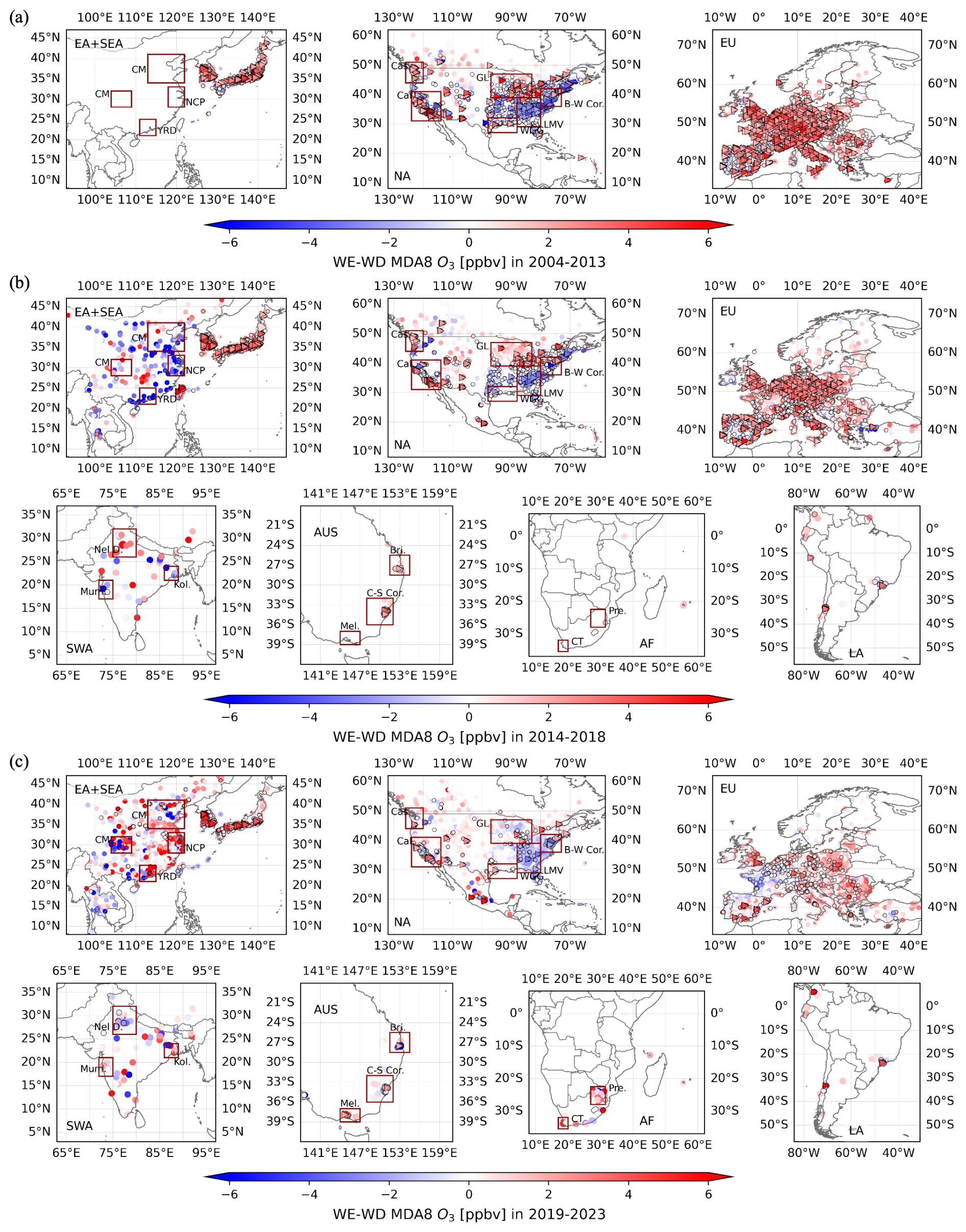
Figure 7 2-decade evolution of WE-WD O₃ differences across three distinct periods: (a) 2004–2013, (b) 2014–2018 and (c) 2019–2023. Significant (p value of t test<0.05) WE-WD O₃ differences and WE-WD NO₂ differences are denoted by triangles and black-edged symbols, respectively.

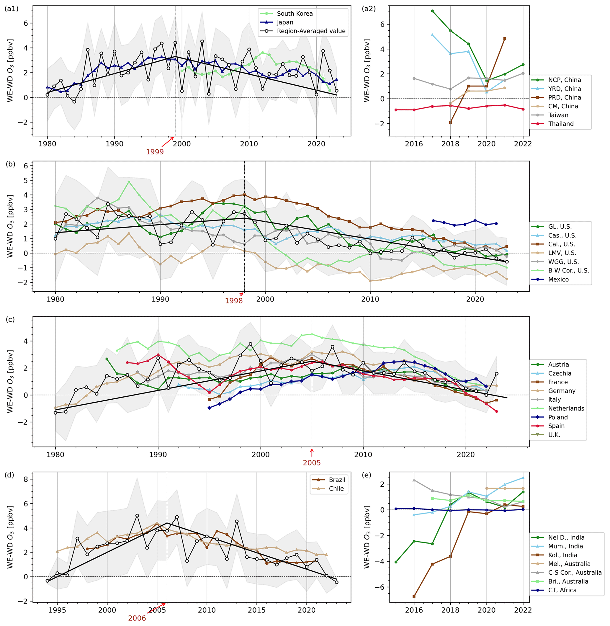
Figure 8 Long-term trends of WE-WD O₃ trends across major economic regions (see Fig. 3a for locations) and selected countries using TOAR data (>100 sites). All sites with ≥10 years of data are included in the continental region-averaged statistics (black line), and sites with ≥3 years of data are included in the major economic regions and selected countries statistics.

3.3.1 Disappearing WE-WD O₃ effect in highly developed regions

Over the past 2 decades, significant NO₂ reductions have been observed globally, accompanied by a persistent but weakening weekend NO₂ dip (Fig. S1). This decline in NO_x availability has systematically altered the weekend O₃ pattern, as evidenced by Theil–Sen regression analyses showing statistically significant (p<0.05) negative trends in WE-WD O₃ across most monitoring sites (Fig. S5). The phenomenon is particularly pronounced in North America; Europe; and developed East Asia regions, such as Japan, South Korea and Taiwan. For example, in Europe, more than 70 % of TOAR monitoring sites exhibited significant weekend O₃ increases before 2013 (Fig. 7a), but by 2019–2023, only 2 % of sites still showed such an effect (Fig. 7c).

The consistent alignment between WE-WD O₃ trends and $\mathrm{HCHO}/{\mathrm{NO}}_{\mathrm{2}}$ ratio evolution provides robust evidence for O₃ regime transitions. This coherence is particularly evident in the temporal correspondence between reversal points – where WE-WD O₃ reductions either coincided with or slightly lagged behind the reversal points in $\mathrm{HCHO}/{\mathrm{NO}}_{\mathrm{2}}$ trends. Early-industrialized regions were already in typical VOC-limited regimes by 1996 (significant positive WE-WD O₃ and low $\mathrm{HCHO}/{\mathrm{NO}}_{\mathrm{2}}$) and have demonstrated a clear transition toward NO_x-limited conditions (decreasing WE-WD O₃ and increasing $\mathrm{HCHO}/{\mathrm{NO}}_{\mathrm{2}}$) since the late 1990s. North America shows peak WE-WD O₃ differences (2.5 ± 1.1 ppbv) during 1995–2000, concurrent with accelerating $\mathrm{HCHO}/{\mathrm{NO}}_{\mathrm{2}}$ growth. Similarly, Europe's aggregated WE-WD O₃ maximum (∼2005) following continental-scale $\mathrm{HCHO}/{\mathrm{NO}}_{\mathrm{2}}$ increases. This lag reflects the causal sequence where $\mathrm{HCHO}/{\mathrm{NO}}_{\mathrm{2}}$ changes drive regime shifts that subsequently manifest in WE-WD O₃ trends. In East Asia, long-term O₃ observations are available mainly for Japan and South Korea. Japanese data show a peak WE-WD O₃ (3.3 ± 0.5 ppbv) around 1999 (Fig. 8a1), while South Korea's maximum occurred later (∼2012).

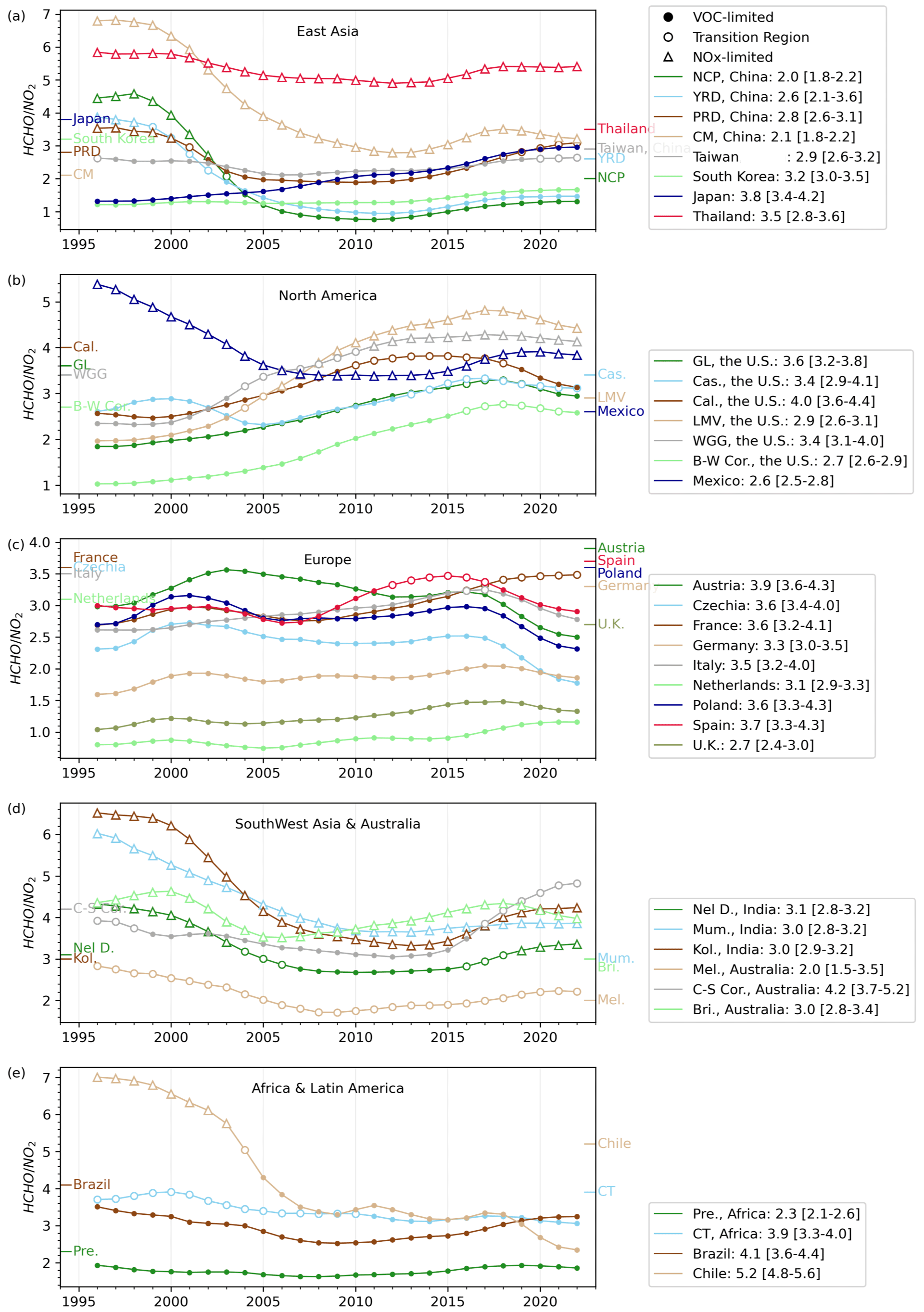
Figure 9 Temporal evolution of tropospheric $\mathrm{HCHO}/{\mathrm{NO}}_{\mathrm{2}}$ ratios by region, with symbols indicating annual O₃ regimes: VOC-limited (solid circle), transitional range (open circle) and NO_x-limited (open triangles). Regional peak threshold values ($\stackrel{\mathrm{̃}}{x}$, marker on y axis) correspond to Fig. 3c definitions.

Post-1996 acceleration in $\mathrm{HCHO}/{\mathrm{NO}}_{\mathrm{2}}$ ratios across North America and Europe preceded partial transitions from VOC-limited to transitional regimes (2011–2016), observed in regions like California, Cascadia, the US BW Corridor, Spain and France. However, complete transitions to NO_x-limited conditions remained rare, except in high-biogenic-VOC regions like the southeastern US (LMV and WGG). Sporadic negative WE-WD O₃ (Fig. 7b and c) indicates emerging NO_x sensitivity, though there is a lack temporal consistency. By 2023, most regions retained either strong VOC-limited regimes (e.g., most European countries, Japan and South Korea) or transitional states (e.g., US BW Corridor) (Fig. 9a–c). Notably, early transitioning regions (e.g., California) showed secondary shifts toward weakened VOC-sensitivity, characterized by near-zero WE-WD O₃ (±1 ppbv) and $\mathrm{HCHO}/{\mathrm{NO}}_{\mathrm{2}}$ ratios approaching the transitional range lower bound (x_lower), indicating persistent VOC-dominated but NO_x-influenced chemistry.

3.3.2 Delayed transition pathways in rapidly developing economies

O₃ production regimes in later-industrialized economies exhibit a temporal lag in evolutionary pathways compared to developed regions. China completed its monitoring network around 2017, coinciding with stringent emission control policies at the same period. Consequently, observed WE-WD O₃ trends align with the global pattern of declining O₃ weekend effects (Fig. 8a2). Satellite-derived $\mathrm{HCHO}/{\mathrm{NO}}_{\mathrm{2}}$ ratios provide crucial complementary data, revealing that eastern China's megacity clusters (NCP and YRD) underwent a dramatic regime shift from NO_x-limited to VOC-limited conditions during 1998–2005, with ratios plummeting from >4 to ∼1.2 (−0.56 yr⁻¹). Despite modest post-2011 recovery (<0.1 yr⁻¹) under emission controls, most Chinese regions remain VOC-limited.

India presents a distinctive case where persistent NO_x-limited conditions prevail across most regions, driven by unique climatic and emission characteristics. Major urban centers, including Delhi, Mumbai and Kolkata experienced significant $\mathrm{HCHO}/{\mathrm{NO}}_{\mathrm{2}}$ ratio declines during the late 1990s, followed by gradual recovery after 2011. While the Delhi Metropolitan Area exhibits fluctuations suggesting potential regime shifts; however, the relatively late establishment of comprehensive monitoring networks (around 2015) introduces uncertainty in determining precise threshold values for regime classification in this region. For most of India, despite large anthropogenic NO_x emissions, India's hot, humid climate enhances biogenic VOC emissions (Kuttippurath et al., 2022), leading to a NO_x-limited dominated regime.

Economies such as those of Australia and Latin America exhibit intermediate patterns. Australian urban areas display varied regime behaviors: Melbourne remains transitional, the Canberra–Sydney Corridor fluctuates near VOC-limited thresholds, and Brisbane maintains NO_x-limited conditions due to a lower anthropogenic influence (Fig. 9d). WE-WD O₃ trends confirm these classifications, with most Australian sites showing insignificant weekend high O₃ in recent years.

In Latin America, developed areas like Brazil and Chile recorded peak WE-WD O₃ (∼4 ppbv) around 2006, coinciding with minimum $\mathrm{HCHO}/{\mathrm{NO}}_{\mathrm{2}}$ ratios around the year. Urban Brazil has kept consistently VOC-sensitive. Chile, however, underwent a dramatic transition – from strongly NO_x-limited conditions ($\mathrm{HCHO}/{\mathrm{NO}}_{\mathrm{2}}\sim \mathrm{7}$) in 1996 to VOC-limited regimes by 2005 – mirroring the initial trajectory observed in eastern China but without subsequent recovery. By 2018, Chile's $\mathrm{HCHO}/{\mathrm{NO}}_{\mathrm{2}}$ ratio even showed accelerated decline, maintaining WE-WD O₃>0 with no signs of transit.

South Africa's Cape Town demonstrates remarkably stable $\mathrm{HCHO}/{\mathrm{NO}}_{\mathrm{2}}$ ratios over the past 27 years, showing minimal temporal variation (coefficient of variation <10 %). This stability maintains quasi-transitional O₃ production conditions (WE-WD O₃≈0 ± 0.5 ppbv), indicating a near-equilibrium state between NO_x and VOC sensitivities.

Globally, the inverse correlation between WE-WD O₃ and $\mathrm{HCHO}/{\mathrm{NO}}_{\mathrm{2}}$ ratios reveals consistent regime evolution patterns. Industrialized regions show widespread weakening of VOC-limited conditions, with most now being transitional or weakly VOC-limited (WE-WD O₃≈0 ± 1 ppbv). In contrast, developing regions that rapidly shifted from NO_x-limited to VOC-limited conditions in the late 1990s have shown incipient reversals since 2011, though most remain firmly VOC-limited. These findings demonstrate that O₃ chemical regimes continue to undergo global-scale transitions, with progression rates modulated by regional emission trajectories and environmental factors.

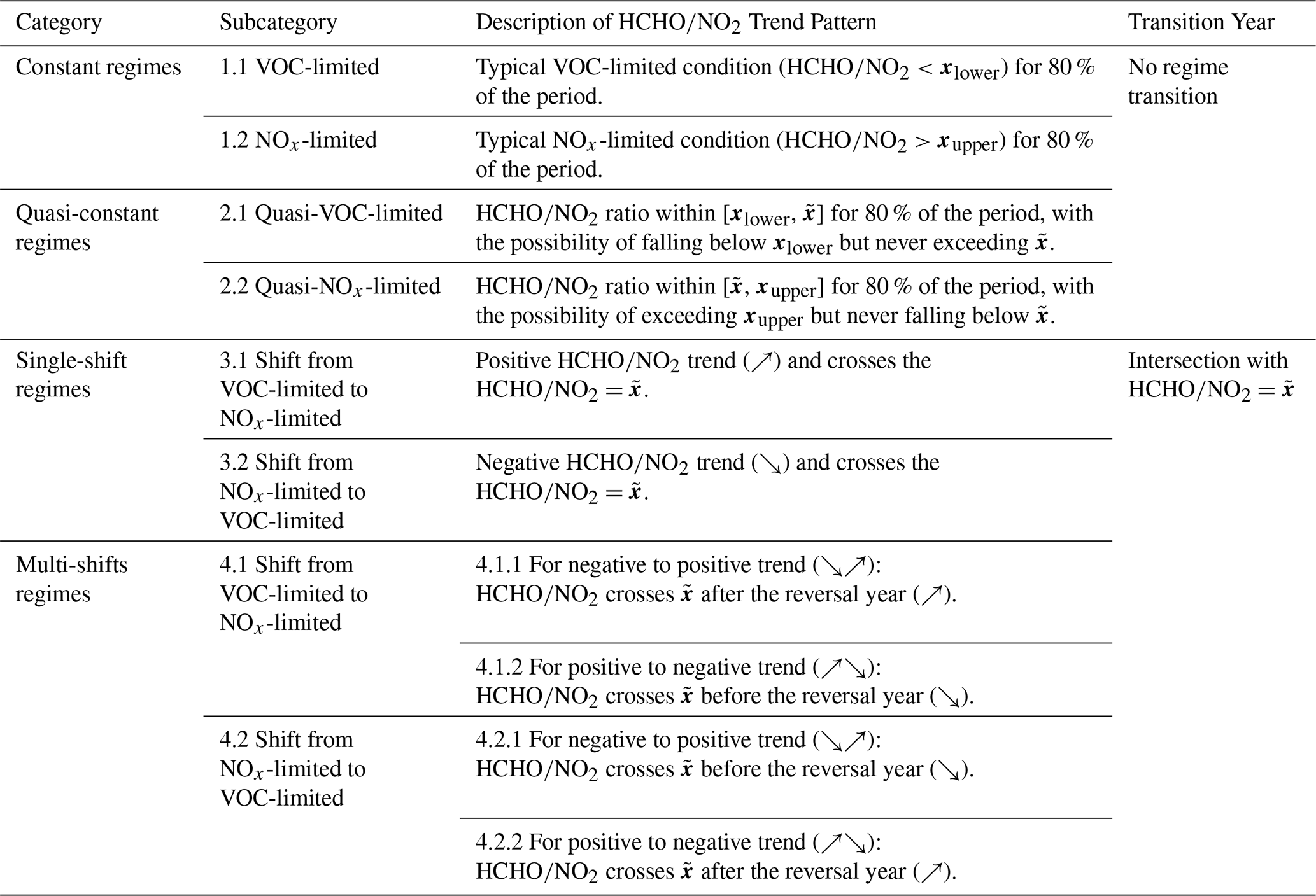
Table 1 Classification criteria for O₃ regime transitions based on three key parameters for each region: peak $\mathrm{HCHO}/{\mathrm{NO}}_{\mathrm{2}}$ threshold frequency ($\stackrel{\mathrm{̃}}{\mathit{x}}$), transition threshold interval [x_lower–x_upper] defined by the top 10 % frequency distribution.

3.4 Global spatiotemporal evolution in O₃ chemical regimes: transition status and potential transition years

Building on our analysis of O₃ regime transitions across economic regions, we refine the regional aggregation approach by implementing a gridded analytical framework. To ensure accuracy, we employ region-specific thresholds derived from Fig. 3b to identify potential transition years. This generates a spatially explicit classification map of regime evolution across the 27-year study period (1996–2022), where each grid cell is categorized into four distinct types based on $\mathrm{HCHO}/{\mathrm{NO}}_{\mathrm{2}}$ ratios trend and regional key threshold ranges: (1) constant-regime grid cell, which stays in either VOC-limited or NO_x-limited regimes without transition; (2) quasi-constant-regime cell, which is predominantly in one regime but intermittently approached the upper or lower limit of threshold range; (3) single-shift-regime cell, which had one directional shift between VOC- and NO_x-limited states during the study period; and (4) multi-shift-regime cell, which had nonlinear trends with threshold crossings in both directions. This classification takes into account the initial conditions of O₃ regimes and their transitional characters based on the observed $\mathrm{HCHO}/{\mathrm{NO}}_{\mathrm{2}}$ trends. Table 1 outlines the diagnostic criteria and the methodology for identifying transition years. Applying the classification rules from Table 1 to global grid cells, Fig. 10 illustrates the spatial distribution of O₃ regime changes. Only areas with a significant anthropogenic influence (NO₂ vertical column density $>\mathrm{1.5}\times {\mathrm{10}}^{\mathrm{15}}$ molecules cm⁻²) are shown here.

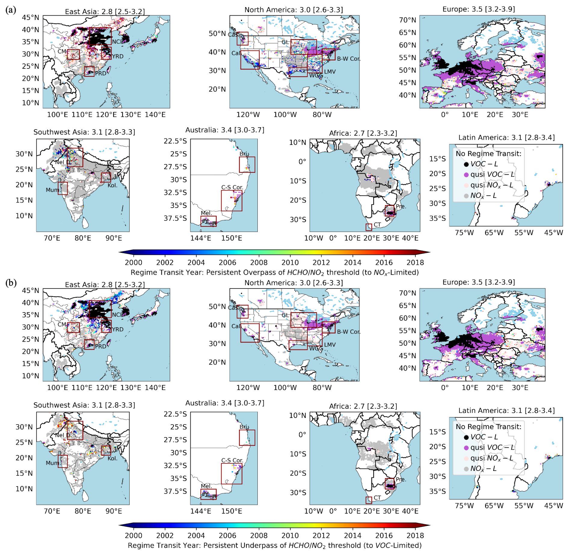
Figure 10 Spatial distribution of estimated transition years for O₃ regime shifts based on annual $\mathrm{HCHO}/{\mathrm{NO}}_{\mathrm{2}}$ ratios crossing region-specific thresholds (identified in Fig. 3b). Panels show (a) grids with positive trends (categories 3.1, 4.1.1 and 4.2.1 in Table 1) and (b) grids with negative trends (categories 3.2, 4.1.2 and 4.2.2). Only grids with long-term mean NO₂ VCD $>\mathrm{1.5}\times {\mathrm{10}}^{\mathrm{15}}$ molecules cm⁻² are shown. Color coding indicates constant VOC-limited (black, category 1.1), constant quasi-VOC-limited (purple, category 2.1), constant quasi-NO_x-limited (pink, category 2.2) and constant NO_x-limited (gray, category 1.2) categories.

Despite varying $\mathrm{HCHO}/{\mathrm{NO}}_{\mathrm{2}}$ trends, many central economic zones remain VOC-limited or quasi-VOC-limited, with $\mathrm{HCHO}/{\mathrm{NO}}_{\mathrm{2}}$ ratios rarely exceeding the upper limit of the threshold range (x_upper). Key regions exhibiting long-term typical VOC-limited dominance include China's NCP, YRD and PRD; metropolitan areas in west Taiwan, South Korea and Japan; US East Coast and California's Los Angeles and San Francisco regions; southern UK; the Netherlands; Belgium; northern France; central-western Germany; northern Italy; New Delhi area (India); Pretoria area (South Africa); and Rio de Janeiro area (Brazil). Quasi-VOC-limited conditions prevail in several regions, including the southern Great Lakes area in the US, much of central-western Europe, Melbourne and the C–S Corridor area (Australia), the Santiago metropolitan area (Chile), and Buenos Aires area (Argentina). In contrast, NO_x-limited or quasi-NO_x-limited regimes dominate southern China (except the highly developed YRD and PRD), lower reaches of Mississippi River Basin in the US, large parts of India and the Congo Basin – regions characterized by distinct climatic and emission profiles.

In regions with significant human activity, transitions to VOC-limited regimes generally precede those to NO_x-limited regimes. Notable VOC-limited transitions are identified between 2000 and 2005 in peripheral zones of China's NCP and the middle-lower Yangtze River regions (Fig. 10b). The entire NCP transitioned to VOC-limited conditions around or slightly before this period, but persistent strong VOC-limited dominance led to its classification as a typical VOC-limited region. NO_x-limited transitions exhibit an urban–rural gradient, with megacity peripheries shifting first and progression inward – a pattern particularly evident in Los Angeles and San Francisco (North America region in Fig. 10a). Regions showing clear transitions to NO_x-limited regimes include part of central Honshu (Japan), mid-southern California, parts of the southeast US and scattered areas in Europe (e.g., part of Spain and France), primarily between 2000 and 2010.

In summary, between 1996 and 2022, most highly developed regions remained consistently VOC-limited or quasi-VOC-limited. Although a global shift toward NO_x-limited conditions is emerging, full transitions remain rare, with only isolated cases in parts of central Honshu in Japan, California and southeast US, and certain European regions. Note that the regime threshold values are subject to large uncertainties due to factors such as meteorological conditions and satellite detection noise (Souri et al., 2020, 2017; Jin et al., 2017; Schroeder et al., 2017). The key $\mathrm{HCHO}/{\mathrm{NO}}_{\mathrm{2}}$ threshold used here is derived from observation sites from the TOAR network that tend to be in urban or accessible areas, which is more reflective of regions with significant human impact rather than pristine natural environments. These factors have the potential to bias the estimated transition year. However, such bias is not significant. It is estimated that a ∼10 % variation in the threshold (e.g., from 3 to 3.3) would shift the estimated transition years by only about 1–2 years for the major global regions. The uncertainty introduced by this simplified approach is considered acceptable.

4 Conclusion

In this study, satellite-derived $\mathrm{HCHO}/{\mathrm{NO}}_{\mathrm{2}}$ ratios and ground-based O₃ observations are directly connected to capture the nonlinearity of global shifts in O₃ chemical regimes. The key findings are as follows.

The evolution of O₃ regimes is discernible through the analysis of the $\mathrm{HCHO}/{\mathrm{NO}}_{\mathrm{2}}$ ratio and WE-WD O₃ trends. We have pinpointed broadly similar but regionally modulated threshold ranges of 2.8 [2.5–3.2] for East Asia, 3.0 [2.6–3.3] for North America, 3.5 [3.2–3.9] for Europe, 2.9 [2.7–3.2] for Southeast Asia, 3.1 [2.8–3.3] for Southwest Asia, 3.4 [3.0–3.7] for Australia, 2.7 [2.3–3.2] for Africa and 3.1 [2.9–3.4] for Latin America. These thresholds are shaped by variations in regional emission profiles.

Amidst the ongoing changes in the ratios of O₃ precursors, a global trend towards NO_x-limited O₃ regimes has emerged over the past 2 decades. This is evidenced by both the rising $\mathrm{HCHO}/{\mathrm{NO}}_{\mathrm{2}}$ ratios and the diminishing O₃ weekend effect, particularly in densely populated regions. Applying linear fitting and reversals analysis, we have observed a predominantly positive or negative-to-positive shift global trend in the $\mathrm{HCHO}/{\mathrm{NO}}_{\mathrm{2}}$ ratio over the past 27 years. Later-industrialized regions like East China and India initially saw a decline before rebounding around 2011; industrialized nations like the US, Europe and Japan experienced significant increases in the $\mathrm{HCHO}/{\mathrm{NO}}_{\mathrm{2}}$ ratio from the early 2000s due to substantial NO_x emission reductions. By 2023, most regions' annual-mean $\mathrm{HCHO}/{\mathrm{NO}}_{\mathrm{2}}$ ratios have not significantly surpassed the key threshold, indicating they remain within VOC-limited or transitional regimes. However, O₃ chemical regime varies seasonally, and we expect the regime transition has occurred during the warm season when O₃ pollution is highest. Regarding WE-WD O₃, while some regions like France and northern Spain show lower weekend levels, the majority still report slightly higher weekend O₃ on an annual basis, but these increases are not statistically significant anymore. A few areas, such as the southeastern US, heavily influenced by biogenic VOCs, have clearly entered an NO_x-limited regime on an annual basis. These results align with the general trend of weakening VOC-limited conditions.

Our findings provide valuable insights into global O₃ regime transitions. By employing region-specific threshold ranges, we demonstrate that early-industrialized nations benefit most from integrated NO_x–VOC controls, as both precursors contribute significantly to O₃ formation in their transitional regimes. For later-industrialized regions, prioritizing NO_x reductions remains critical to avoid entrenched VOC-limited conditions. This framework highlights the necessity of adaptive emission strategies that account for both chemical regime shifts and development stages. However, it should be noted that using satellite $\mathrm{HCHO}/{\mathrm{NO}}_{\mathrm{2}}$ to diagnose O₃ production regimes is subject to uncertainties of satellite retrievals and the regime threshold values. We use tropospheric NO₂ and HCHO column densities to infer near-surface O₃ chemistry, but this approach is influenced by variable column-to-surface relationships driven by boundary layer dynamics and contributions from the free troposphere (Dang et al., 2023; Wolfe et al., 2019; Jin et al., 2017). For the regions with decreasing NO₂ in particular, the contribution of free tropospheric NO₂ is likely to increase (Dang et al., 2023), which could bias the observed trends of $\mathrm{HCHO}/{\mathrm{NO}}_{\mathrm{2}}$. Here, we focus on O₃ regime evolution annually, but the O₃ regime also varies seasonally and diurnally. How the seasonal and diurnal variations in the O₃ regime have evolved over time warrants further investigation. Further research could employ chemical-transport modeling to better understand both the seasonal influences and the physical drivers of regional threshold differences, for instance, examining why economically developed regions are characterized by higher values compared to less industrialized areas.