A conceptual framework for understanding longwave cloud effects on climate sensitivity

We add idealized clouds into a single-column model and show that cloud radiative effects, as observed from satellites, can be reproduced by a combination of high- and either low- or mid-level clouds. To quantify all-sky climate sensitivity, we adopt the “fixed-cloud-albedo” ansatz as the null hypothesis for climate sensitivity. Our ansatz assumes an understanding of how clouds distribute themselves in temperature space, but it assumes no change in cloud albedo. Drawing only distributions which match the cloud radiative effects of present-day observations yields a mean fixed-albedo climate sensitivity of 2.2 K (also keeping surface albedo fixed), slightly smaller than its clear-sky value. This small number arises from two compensating effects: the dominance of cloud masking of the radiative response, primarily by mid-level clouds, which are assumed not to change with temperature, and a reduction in the radiative forcing due to the masking effect by high clouds. Giving more prominence to low-level clouds, which are assumed to change their temperature with warming, reduces estimates of the fixed-albedo climate sensitivity to 2.0 K. This provides a baseline to which changes in surface albedo and a presumed reduction in cloud albedo would add to.

1 Introduction

The cloud radiative effect is a significant contributor to Earth's radiation balance (Hartmann and Short, 1980; Ramanathan et al., 1989). In the net it leads to a cooling of Earth's surface as the contribution of clouds to the planetary albedo, through scattering of visible radiation, is larger than their greenhouse effect, arising from their absorption of terrestrial radiation (Loeb et al., 2018). A stronger cloud albedo effect is expected because the minimum temperature of the troposphere and hence clouds is much larger than zero, which more tightly bounds the cloud greenhouse effect. This gives changes in cloud albedo greater scope for influencing climate sensitivity and explains why they are the subject of increased study (Ceppi et al., 2017).

While cloud albedo effects arise from changes in cloud microphysical properties and/or spatial extent, cloud greenhouse effects also depend on cloud-top temperature. This means that even under the ansatz of a fixed cloud albedo, the mere manner by which clouds distribute themselves in temperature space may influence Earth's equilibrium climate sensitivity. Two effects can be identified that correspond to masking of the radiative response to forcing or warming: for the former, high clouds mask the radiative forcing in spectral regions (wavenumbers) where CO₂ emissions would otherwise arise from regions below the clouds. At these wavenumbers, and in these situations, the changing emission height arising from an increase in CO₂ will not be apparent at the top of the atmospheres – clouds get in the way. For the latter, clouds modify the radiative response to warming by masking emissions in the spectral region known as the atmospheric window and by unmasking parts of the spectral response that they would have otherwise masked or which would have been masked by water vapor (McKim et al., 2021; Jeevanjee, 2023; Stevens and Kluft, 2023). The cloud masking of CO₂ forcing is well appreciated and accounted for in the literature (Myhre et al., 1998), while masking or unmasking of the clear-sky spectral response (Stevens and Kluft, 2023) is not.

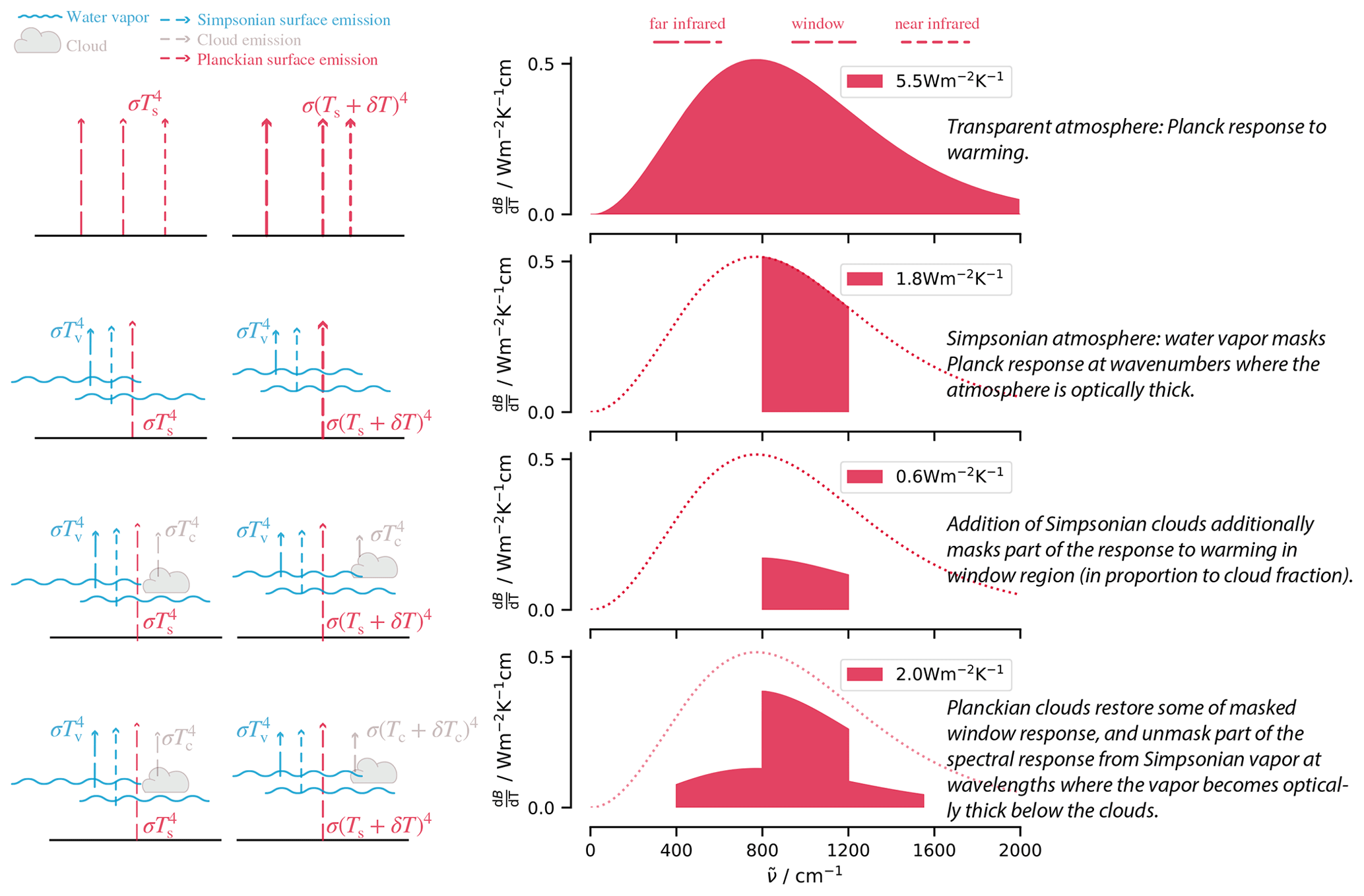
Figure 1 Conceptual framework showing how Simpsonian clouds and water vapor mask the radiative response at wavenumbers where they control the emission to space and how part of the spectral response is restored by Planckian clouds.

The basic idea of cloud masking is illustrated with the help of the schematic in Fig. 1. For simplicity the schematic leaves out the effects of CO₂ and other long-lived greenhouse gases (see, e.g., Raghuraman et al., 2024). Later, in our more detailed computations, these effects are included. We define the atmospheric window as the range of wavenumbers (800–1200 cm⁻¹) where the atmosphere is optically thin throughout the entire column. Outside of this window, emission of radiant energy to space arises from water vapor (and from CO₂ or other long-lived greenhouse gases, were they to be considered). In these regions, the assumption of fixed relative humidity means that the optical thickness of the atmosphere, as measured downward from the top of the atmosphere, depends on temperature, and hence emissions will not change with surface warming. We refer to this as a Simpsonian response (Ingram, 2010; Jeevanjee et al., 2021), which can be conceptualized as a spectral masking of the Planckian response that would otherwise arise from the surface (Fig. 1, second row). Clouds, unlike water vapor, are gray across the thermal infrared. They thus control emissions at wavenumbers where the clear-sky emission would otherwise originate below them. Whether, and how much, they contribute to the radiative response to warming then depends on how or if they warm with the surface. Clouds which maintain a fixed temperature (Simpsonian clouds) mask the spectral response that otherwise would have been expected in the window – reducing the radiative response to surface warming. Clouds that warm with the surface (Planckian clouds) can substitute for the surface response within the window. If the change in cloud temperature is equal to the change in the surface temperature, then this mimics the surface response, albeit somewhat weakened by virtue of the clouds being at lower temperatures. Outside of the window, at wavenumbers where the emission height of water vapor lies below the clouds, the warming clouds can reclaim part of the spectral response which would have otherwise been masked by water vapor (Stevens and Kluft, 2023), as shown in the last row of Fig. 1.

Understanding the radiative effect of how clouds distribute themselves in temperature space is a prerequisite for understanding climate sensitivity, as these effects temper the radiative forcing from greenhouse gases and the radiative response to warming, even in cases where the spatial coverage and microphysical properties of clouds do not change with warming. Previous studies, of course, include these effects, but they are rarely separated from the clear-sky response. For instance, a common approach to disentangling the cloud feedback is the partial radiative perturbation (PRP) method (Colman, 2003; Soden and Held, 2006). This method performs radiative transfer calculations with different atmospheric fields (e.g., temperature, humidity, clouds) independently varied, with the idea that this quantifies their impact on the radiation budget. Doing so differentiates the effects of changing different variables in coupled models but ignores the cross-dependencies between variables. As a result, the contribution to the radiative response from water vapor, as estimated by the PRP method, will depend on the assumed distribution of clouds; likewise adding and subtracting a given distribution of clouds will give different answers depending on the background distribution of water vapor.

In this study we follow Stevens and Kluft (2023) to explicitly account for the masking and unmasking of the spectral response of outgoing radiant energy to surface warming, or CO₂ forcing, under the fixed-cloud-albedo ansatz. We begin by providing a precise description of the atmospheric thermodynamic structure, including its clouds, and how this will change with warming. We then calculate the changes in the irradiances with surface warming (or CO₂ forcing) for an atmosphere with and without clouds. Precision of description is facilitated by the use of the single-column model konrad (Kluft et al., 2019; Dacie et al., 2019), under the fixed-cloud-albedo ansatz. That is, we assume that spatial coverage of clouds and their microphysical properties do not change with warming. Our approach extends a growing body of literature using simple models under well-defined limits to better understand the climate sensitivity of a cloud-free atmosphere by including the effects of clouds (e.g., Koll and Cronin, 2018; Seeley and Jeevanjee, 2021; Kluft et al., 2021; Jeevanjee et al., 2021; Jeevanjee, 2023; Feng et al., 2023; Koll et al., 2023; Roemer et al., 2023; Stevens and Kluft, 2023). Using a single-column model in this manner is admittedly simplistic, but because the radiative response varies linearly with the main state variables (Koll and Cronin, 2018; Bourdin et al., 2021; Kluft et al., 2021), the response of the mean state has proven to be quantitatively informative of the mean response to a spatially varying state. More fundamentally, our approach allows for transparency of reasoning, which aids the interpretation of results from more complex settings and as such is fundamental for improving our understanding (Shaw and Stevens, 2025).

The methodology of our calculations is provided in Sect. 2. In Sect. 3 we discuss the simulated cloud radiative effect in present-day conditions and the effect of prescribed cloud changes to warming. Section 4 discusses the aspects in which our perspective on cloud feedbacks differs from or accords with existing frameworks. Section 5 summarizes the conclusions of our study.

2 Modeling the effects of clouds in one dimension

We quantify the radiative effect of clouds using konrad, a Python-based one-dimensional radiative–convective equilibrium (RCE) model (Kluft et al., 2019; Dacie et al., 2019). Clouds at three levels are considered.

It is doubtful whether one can unambiguously construct a “global cloud scene” that can be used within konrad to best represent cloud effects on the radiative response to warming or forcing. Many of the physical properties of clouds are still poorly quantified, and even if they were well known, the aggregation of these properties for application in a simple one-dimensional model would entail ambiguity, as different representations might be better adapted to different purposes. Hence we approach the problem functionally by creating a large ensemble of plausible cloud properties for the three layers of clouds considered, and we select configurations consistent with global mean cloud radiative effects as observed from space (Clouds and Radiant Energy Systems, CERES; Loeb et al., 2018). Both the full ensemble of cloud properties and the plausible subsample are then used to quantify the cloud masking effect on the radiative forcing and its masking/unmasking effect on the radiative response to warming.

Calculations with konrad are performed by prescribing the surface temperature. The tropospheric temperature profile is adjusted to a moist adiabat corresponding to the surface temperature. Above the convective top, which is the uppermost level that requires convective adjustment, the temperature profile is equilibrated into a radiative equilibrium, which allows us to capture changes in cold-point temperatures. This approach greatly reduces the computational burden as it avoids the need to equilibrate the surface temperature (Romps, 2020). The relative humidity (RH) is modeled as a C-shaped profile, as roughly observed in the tropics. The RH profile is kept constant in temperature space, thus adjusting its vertical structure as the troposphere expands (Romps, 2014). For simplicity, we approximate the RH profile using a piecewise linear function of temperature T. It is specified to have a value of 80 % at T≥283 K, decreasing to a minimum of 40 % at 250 K and increasing back to a value of 80 % at T≤200 K.

All-sky fluxes are calculated using a two-stream correlated-k representation of radiative transfer, RRTMG (Mlawer et al., 1997). Our previous work has shown RRTMG to compare well against line-by-line calculations within this same framework and for the temperature ranges considered here (Kluft et al., 2021). RRTMG computes fluxes for completely overcast or clear-sky scenes. In overcast scenes, clouds are represented in terms of their pressure and temperature, optical depth, single-scattering albedo, and asymmetry parameter, with the optical properties represented as a function of an assumed cloud phase, a condensate burden, and an effective radius. All-sky fluxes are constructed by weighted averages between clear and overcast scenes, depending on the fractional weight of each.

The three layers of clouds are endowed with distinct physical properties and behaviors as follows. A low-level cloud layer is introduced to represent boundary layer clouds, and its cloud-top temperature changes following a fixed anvil pressure (FAP), which, due to the assumption of the moist adiabat, means they will warm slightly more than the surface¹; a mid-level cloud layer is introduced at the melting level and is assumed to maintain a fixed anvil temperature (FAT); and a high-level cloud layer is introduced following the proportionally higher-anvil-temperature (PHAT) hypothesis, in which clouds are tied to the level of the maximum of the radiatively driven convergence in clear skies (Zelinka and Hartmann, 2010; Bony et al., 2016). This approach allows the cloud altitude to be precisely defined for different background climates. Therefore, we can use two simulations with differing surface temperatures T_s=285 K and 291 K to compute the radiative feedback, including the cloud–altitude feedback. The somewhat high value of ΔT_s=6 K is intended to give a clear signal of changes in cloud-top height, which can only be changed by full model levels.

We assume that the overlap among clouds in different layers is random, which defines 2³ different cloud configurations – each of which can lead to markedly different cloud radiative effects. In global circulation models (GCMs), this variability is parameterized by, e.g., the Monte Carlo independent column approximation (McICA; Pincus et al., 2003). This is effective when the radiation scheme is called often in time, as the sample noise is unbiased and averages out with high-temporal sampling. For our purposes, the limited number of cloud layers, and hence the smallness (2³) of the configuration space, allows for a simpler approach. Let i∈{1…8} index each cloud combination such that i=1 denotes clear skies, i=2 denotes only high clouds, and so on, as illustrated in Fig. 2. The probability of a given combination of clouds is then given as

$$\begin{array}{}\text{(1)}& P_i=\prod _{j=\mathrm{1}}^{\mathrm{3}}{P}_{ij},\end{array}$$

with P_ij being the probability that cloud layer j is seen in cloud combination i, which can be expressed as follows:

$$\begin{array}{}\text{(2)}& P_{ij}=|\mathrm{1}-p_j-c_{ij}|,\end{array}$$

where c_ij is the binary cloud flag, in which cloud layer j is present in combination i and the assumed cloud fraction p_j. The resulting weight P_i quantifies the probability of a given cloud combination based on the cloud fraction of the participating cloud layers. The all-sky radiative fluxes are then given by the weighted average of the individual cloud-overcast scenes (Fig. 2).

$$\begin{array}{}\text{(3)}& F=\sum P_i{F}_i\end{array}$$

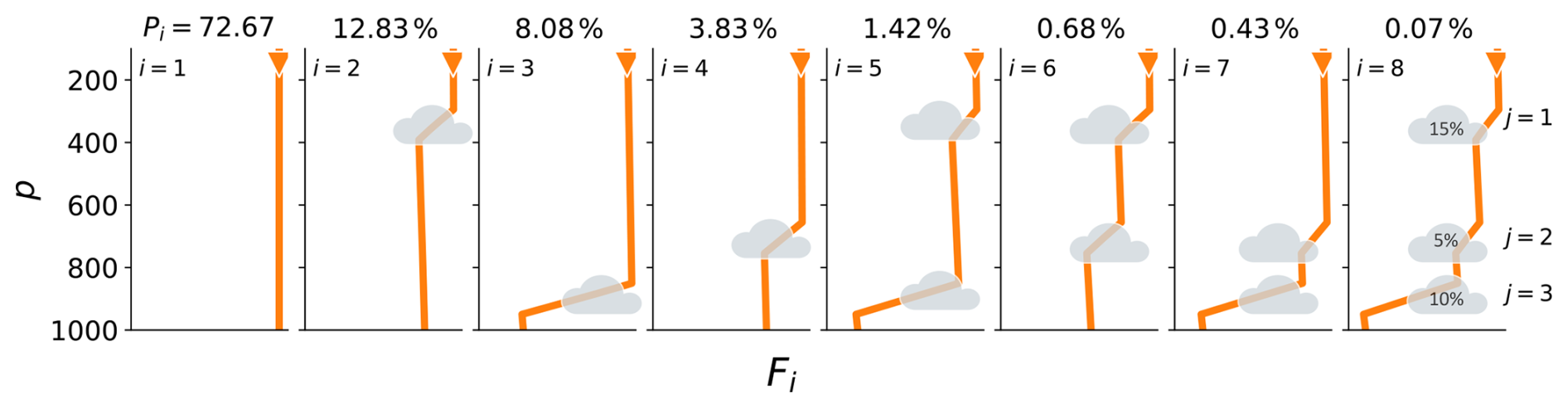
Figure 2 Schematic of all possible cloud layer combinations i in a trimodal cloud distribution. In addition, the different impacts on the downwelling shortwave flux are shown with the orange line. The percentages on top state the probability P_i for each cloud layer combination, assuming random overlap and exemplary cloud fractions (shown in the rightmost panel).

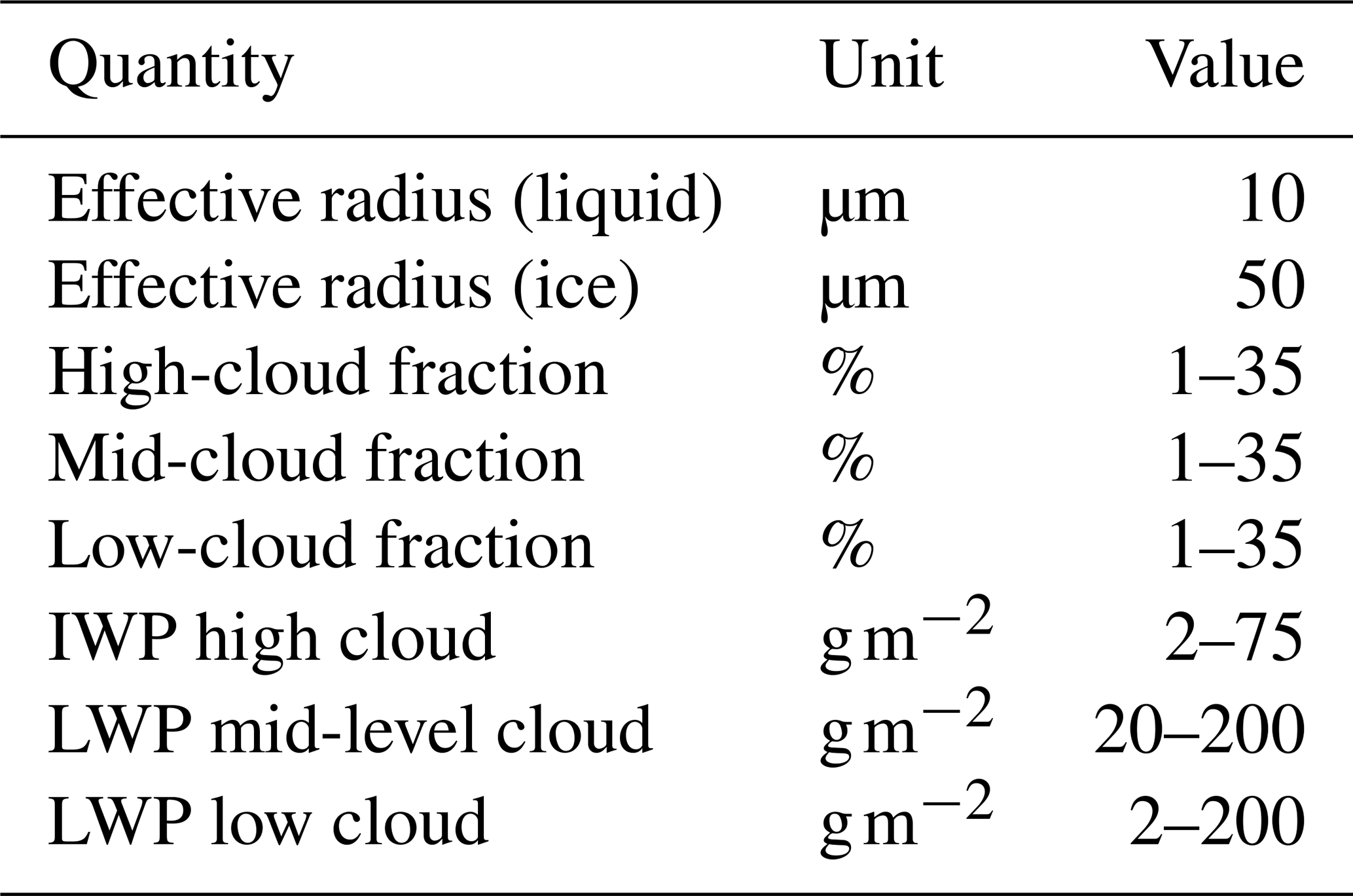
To perform the calculations, we also need to make a choice for the cloud fraction, the integrated condensate path for each cloud layer, and the effective radius. The particle phase, which influences how these physical properties are translated into optical properties, is prescribed for each layer, with low- and mid-level clouds being treated as liquid, high clouds being treated as ice, and no change in the phase of the different layers with warming. We account for ambiguities in the cloud description by using a large Monte Carlo ensemble (MCE), in which we randomly draw parameter values from values taken from a uniform prior distribution over the specified range. These properties are then kept constant from the control and perturbed simulations. The combination of a specified but constant cloud fraction, condensate path, effective radius, and cloud phase, together with the chosen overlap assumption, thus defines our fixed-cloud-albedo ansatz.

Table 1 lists the range of possible values for each cloud property, from which we construct the MCE. We perform 32 768 simulations, each of which comprises 16 radiative transfer calculations (once for the warm and control temperature for each of the 8 configurations), with parameters chosen randomly from the parent distribution. The result is an ensemble of 32 768 cloud scenes that describe the all-sky radiation budgets following the prior distribution of cloud parameters. Many of these scenes will, however, not result in plausible representations of Earth's top-of-the-atmosphere radiation budget, as observed from satellites. Therefore, we construct an a posteriori distribution by subsampling the ensemble to find cloud configurations whose cloud radiative effect (CRE) is consistent with that of satellite observations. This defines a plausible set of cloud scenes, which we then use to quantify various cloud radiative metrics in both the present and a warmer climate.

Table 1 Possible value range for physical and optical cloud parameters in the MCE.

3 Cloud radiative effects

3.1 The current climate

In a first step, we quantify how the presence of clouds impacts Earth's radiant energy budget for the control temperature and use these effects to sample a plausible parameter range for the prescribed clouds. Cloud radiative effects are compared to the summary values for the July 2005–June 2015 period, as provided by the Clouds and Radiant Energy Systems (CERES) EBAF Ed4.0 product (Loeb et al., 2018, Table 5).

Table 2 Plausible value range for cloud amounts in the MCE.

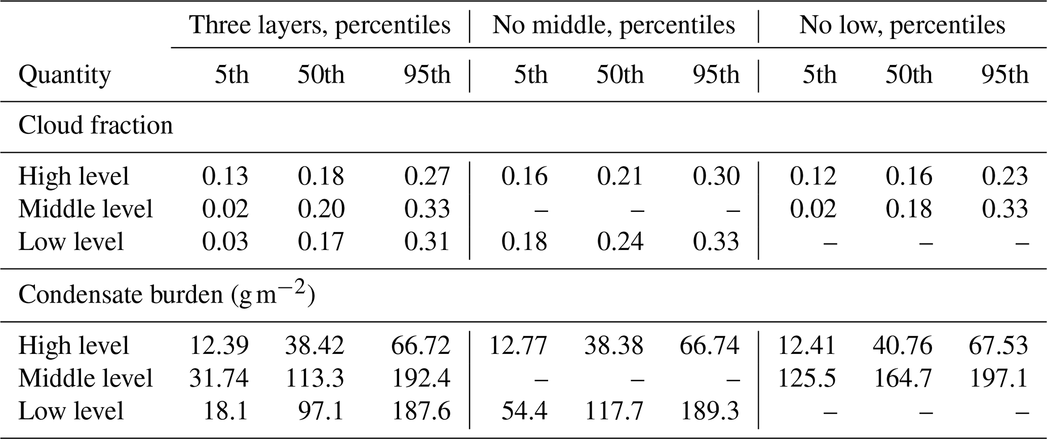
Figure 3 presents the longwave, shortwave, and net CRE for the full ensemble (light colors). Unsurprisingly, values for the net CREs and their components spread across a very large range of values. For example, CRE_net can reach values between −83 and 28 W m⁻². The fact that the ensemble mean is in good agreement with the CERES data suggests that the uniform distributions for the variable parameters were centered around sensible values.

As a next step, we subsample the full ensemble to select cloud configurations in which all three CRE values are within ±5 W m⁻² of the CERES values at the top of the atmosphere – which we refer to as “plausible” values. Tests with narrower acceptance showed no qualitative difference but greatly reduced the output statistics. Even with this relatively loose constraint on acceptable values of the shortwave (SW) (−45.8 W m⁻²), longwave (LW) (27.9 W m⁻²), and net CRE (−17.9 W m⁻²), requiring all three to be satisfied reduces the ensemble to 786 out of 32 786 cloud scenes (about 2.4 %). Parameter distributions for the subset of parameters leading to plausible CREs are described by the 5th, 50th, and 95th percentiles of their distributions and listed in Table 2. The a posteriori distributions show that the CRE from CERES most strongly constrains the property of high-level clouds.

Since the effective parameters found to capture the observed CRE are found to be similar to parameters characteristic of observed clouds, it is justified to use an effective cloud to model the globally averaged effect of broad cloud distributions. The average cloud fraction is 18 % for high clouds, 20 % for mid-level clouds, and 17 % for low clouds, which are not unreasonable values. The coverage of mid-level clouds is higher than expected but could be interpreted as representative of cloud populations in the mid-latitudes. The plausible range for the mid-level and low-level cloud parameters is not substantially reduced relative to their initial distributions, which might be indicative of the capability of the two cloud types to compensate for one another.

To test the possibility of compensation, we further investigate the impact of individual cloud layers by performing three additional sets of simulations. In each of these, we omit one of the three cloud layers. Results are presented in Fig. 3. The strongest impact is seen in the simulation without high clouds. In the absence of high clouds, which are characterized by their cold cloud top, the longwave CRE almost vanishes. As a result, the net CRE is much more negative (about −40 W m⁻² on average) and can no longer be reconciled with the CERES data, and thus we do not plot bold lines in Fig. 3 for the “no-high-cloud” case. The calculations also confirm the ability of increased low-level clouds to compensate for mid-level clouds and vice versa. Table 2 further demonstrates that for two cloud layers, the cloud parameters of the lower cloud layers become more constrained than in the three-layer case. In the absence of either the mid- or the low-level clouds, Fig. 3 indicates that strongly negative CRE_SW values are no longer possible, which makes it more difficult to find samples that reproduce the observed CRE_SW, especially in the absence of low clouds.

We conclude that a single-column model with an idealized trimodal cloud distribution is able to produce CREs that are in good agreement with the best available observations of Earth's radiant energy budget. Our calculations demonstrate that the presence of high clouds is essential for a realistic longwave CRE. While important, low- and mid-level clouds act in a similar way, making it easier for them to compensate for one another. The CRE at the top of the atmosphere is unable to distinguish between low-level and mid-level cloud amounts. This limitation has significant implications for understanding how the system responds to global warming, as modeled in our study. Specifically, our model shows that mid-level clouds mask the radiative response to warming, whereas low-level clouds, which warm in tandem with the surface (as prescribed in the model), are also effective at enhancing the spectral response to warming.

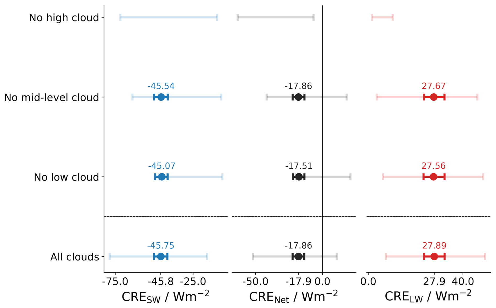
Figure 3 Distribution of the shortwave cloud radiative effect CRE_SW, the net cloud radiative effect CRE_Net, and the longwave cloud radiative effect CRE_LW. The faded lines depict the 5 %–95 % interval of all possible CRE values in the full ensemble. The bold lines show the same range but for a plausible subsample that is in a ±5 W m⁻² range around the mean values from the CERES satellite observations (given as tick labels on the x axis). Different rows of the figure show results for different simulations, in which certain cloud layers were turned off (e.g., the first row describes a simulation with all but high clouds).

3.2 Response to surface warming

In this section we quantify how our representation of clouds modifies the model's clear-sky response to forcing, the radiative response to warming, and their quotient – climate sensitivity.

In exploring how clouds with both a fixed coverage and a fixed albedo (and hence phase) affect the estimate of climate sensitivity, we also explore a form of state dependence, with the cloud distribution being an important state parameter. Past studies, using methods like PRP, would have subsumed these effects into estimates of the clear-sky sensitivity. Our approach allows for a more full accounting of clouds and, by implication, allows us to assess how errors in the distribution of clouds or estimates of changes in cloud temperature will effect estimates of climate sensitivity.

The calculations involve additional simulations based on the MCE of cloud scenes. In a first step, we double the CO₂ concentration while keeping a fixed T_s=288 K. After allowing the stratosphere to adjust to the new gaseous composition, we can directly quantify the adjusted radiative forcing as

$$\begin{array}{}\text{(4)}& \mathrm{\Delta }F=F_{\mathrm{2}\times {\mathrm{CO}}_{\mathrm{2}}}-F_{{\mathrm{CO}}_{\mathrm{2}}},\end{array}$$

with F_x being the outgoing longwave radiation for a CO₂ mixing ratio x.

We find that clouds reduce the radiative forcing by about 0.7 W m⁻² or by about 15 % of the clear-sky value of 4.5 W m⁻² (see bottom row of Fig. 4). This masking is solely done by high clouds because the cloud needs to be located above the emission height of CO₂ to effectively mask the radiative forcing. In the absence of high clouds, ΔF is close to the clear-sky value (see top row of Fig. 4). By constraining our MCE to plausible cloud combinations (bold lines), we find that the reduction in ΔF is a robust signal and, on its own, would reduce the fixed-albedo climate sensitivity by about 0.5 K.

In a second step, we estimate how clouds influence the radiative response to forcing, λ. We quantify this by repeating our simulations at T_s=285 and 291 K. Using the two sets of simulations at different T_s levels, we define the feedback parameter as

$$\begin{array}{}\text{(5)}& \mathit{\lambda }={\displaystyle \frac{F_{\mathrm{291}\mathrm{K}}-F_{\mathrm{285}\mathrm{K}}}{\mathrm{6}\mathrm{K}}},\end{array}$$

with F_T denoting the net irradiance at the top of the atmosphere for the given temperature T.

In each of the simulations, the different cloud levels adjust their cloud-top altitude based on the thermodynamic profiles of the atmosphere (see Sect. 2). This means that low-level clouds remain at the same pressure level, mid-level clouds move upward following the melting level, and high-level clouds move upward following the level where the divergence of the radiatively driven subsidence maximizes. As a result, both high and low clouds warm with the surface, though high-level clouds warm somewhat less, while mid-level clouds remain at the same temperature. The different behavior of mid- and low-level clouds helps quantify to what extent an uncertain temperature response of clouds to surface warming affects the sensitivity of the system to forcing – effectively providing a first estimate of uncertainty introduced by clouds, even if their coverage remains unchanged.

Figure 4b presents λ. Clouds reduce the radiative response to warming, increasing λ from its clear-sky value of −1.9 to −1.7 $\mathrm{W}{\mathrm{m}}^{-\mathrm{2}}{\mathrm{K}}^{-\mathrm{1}}$. This alone would result in an increase in the equilibrium climate sensitivity 𝒮. This effect, however, is less than that of changes in ΔF, which reduces from 4.5 to 3.7 W m⁻². Hence, under the fixed-cloud-albedo ansatz, clouds reduce 𝒮 slightly relative to its clear-sky value. Following the arguments of Stevens and Kluft (2023), this is expected to the extent that clouds unmask parts of the spectral response to warming that would otherwise be masked by water vapor. Comparing the no-mid-level to the no-low-level cloud response shows that low-level clouds are responsible for this unmasking, as in their absence the radiative response to warming is much smaller, and 𝒮 increases by 0.2 K (Fig. 4) over its clear-sky value of 2.3 K. Conversely, in the absence of mid-level clouds, the increase in low-level clouds, which in our model warm slightly more than the surface, enhances the radiative response to warming, reducing 𝒮 by 0.3 K relative to its clear-sky value.

In summary, the net effect on λ is sufficient to balance the reduction in ΔF, resulting in an equilibrium climate sensitivity $\mathcal{S}=-\mathrm{\Delta }F/\mathit{\lambda }$ in the range of 1.94–2.56 K. This range encompasses the clear-sky value of 2.3 K but more often leads to less rather than more warming. This outcome arises because, in our ansatz, the cloud masking effect on ΔF largely compensates for that on λ, while the unmasking effect only influences λ, thereby reducing 𝒮.

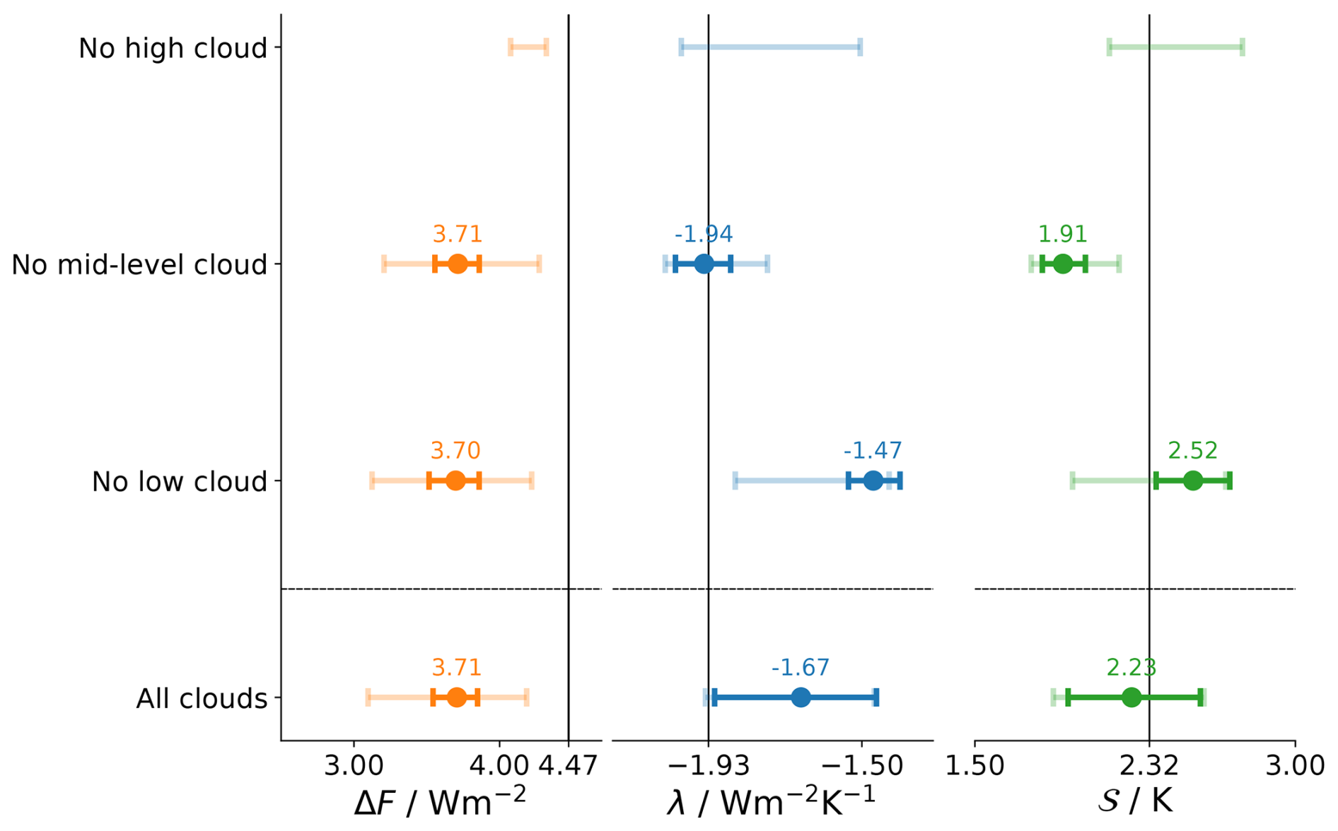
Figure 4 Distribution of the adjusted radiative forcing ΔF, the climate feedback parameter λ, and the equilibrium climate sensitivity 𝒮. The faded lines depict the 5 %–95 % interval of all possible CRE values in the full ensemble. The bold lines show the same range but for a plausible subsample that is in agreement with satellite observations. The vertical lines mark the respective value under clear-sky conditions. Different rows of the figure show results for different simulations, in which certain cloud layers were turned off (e.g., the first row describes a simulation with all but high clouds).

4 Discussion

Readers familiar with traditional cloud feedback analyses might be confused by the estimates of cloud masking in the present study, as compared to estimates in the earlier literature (Colman, 2003; Soden et al., 2008; Yoshimori et al., 2020). These differences reflect differences in how masking is defined. In the earlier studies, cloud masking was introduced to separate the effect of fixed clouds on the radiative response due to changes in non-cloud quantities (temperature, water vapor, etc.) from changes that could be attributed to clouds not being fixed. In the earlier studies, fixed meant fixed in height or pressure. In a warmer climate, fixing clouds in this manner results in more emission from clouds, which is a curious way to think about no change, as it implies a strong enhancement of overall radiative response by fixed clouds. This curious behavior was then more or less canceled once clouds were allowed to change their temperature. A large negative cloud masking was compensated for by a large positive cloud feedback. This side effect of an artificial assumption about what constitutes a fixed cloud is precisely what Yoshimori et al. (2020) set out to address through their introduction of the thermal radiative damping with fixed relative humidity and anvil temperature (T-FRAT) framework. In the T-FRAT framework they identify a small positive cloud feedback, implying that clouds warm more than expected for a fixed anvil temperature. This is consistent with the response of high clouds in the present study. Here too, however, quantitative comparison is difficult, as, in contrast to our framework, which defines the effect of fixed-albedo clouds relative to the cloud-free response, T-FRAT quantifies the effect of cloud changes relative to what would have occurred had clouds maintained a fixed temperature.

One should avoid attaching too much precision to the numbers arising from our calculations. While we can think of myriad ways in which fixed-albedo clouds might distribute themselves in temperature space differently than we have assumed, we do not see arguments that would be indicative of a systematic positive or negative bias. Even without accounting for additional sources of uncertainty in our implementation of the fixed-albedo ansatz – for instance in how clouds overlap, low-cloud warming, or the tendency to place many clouds in the middle troposphere where they are given properties that strongly reduce the radiative response – considerable uncertainty arises merely from the configuration of clouds. This effect leads to an uncertainty of approximately 0.5 $\mathrm{W}{\mathrm{m}}^{-\mathrm{2}}{\mathrm{K}}^{-\mathrm{1}}$ in λ, which quantifies what Yoshimori et al. (2020) called the cloud climatological effect in our model. Observations, combined with three-dimensional calculations using reanalyses, similar to the approach Gloeckner et al. (2025) used to study clear-sky feedback, could help reduce this uncertainty or at least quantify the adequacy of existing cloud climatologies for this purpose.

Even under the fixed-cloud-albedo ansatz clouds can contribute to changes in planetary albedo through their ability to mask surface albedo changes. Pistone et al. (2014) estimate an all-sky radiative response to surface albedo changes that is five-eighths of the clear-sky response – although some of this is likely associated with changes in cloud cover. Thus, an all-sky surface albedo radiative response to surface albedo changes of 0.35 $\mathrm{W}{\mathrm{m}}^{-\mathrm{2}}{\mathrm{K}}^{-\mathrm{1}}$ (Forster et al., 2021) implies a clear-sky surface albedo contribution to the radiative response of 0.56 $\mathrm{W}{\mathrm{m}}^{-\mathrm{2}}{\mathrm{K}}^{-\mathrm{1}}$. Accounting for these changes in our null hypothesis for climate sensitivity gives the best estimate of the fixed atmosphere–albedo clear-sky sensitivity to 3.26 K and the fixed atmosphere–albedo all-sky sensitivity to 2.8 K. This demonstrates that fixed-albedo clouds reduce climate sensitivity even more when surface albedo changes are incorporated.

5 Conclusions

We propose a model for cloud–altitude changes in a warming climate and use this to calculate climate sensitivity under a fixed-cloud-albedo ansatz. Our model allows different cloud types to respond to surface warming in distinct ways: low-level clouds are assumed to be tied to a fixed pressure, mid-level clouds to the freezing level, and high-level clouds to the level of maximum clear-sky subsidence divergence. We add this conceptual representation of clouds to the one-dimensional RCE model konrad to quantify how, if they were to behave in the manner posited, they would affect the radiative response to forcing. The model helps clarify both how cloud temperature changes and how cloud temperature changes of different cloud types influence climate sensitivity, even under the ansatz of a fixed cloud albedo.

Satellite observations show that the presence of clouds cools the current climate by adding a net CRE of about −17 W m⁻². We use this to construct an MCE to demonstrate that a trimodal vertical cloud distribution can adequately simulate the observed CRE, with ambiguity in the distribution of low- versus mid-level clouds. The measurements provide a much stronger constraint to high clouds.

In addition, clouds, even if they do not change their albedo, alter Earth's climate sensitivity, i.e., its warming in response to a CO₂ doubling. On one hand, they mask the radiative forcing by about 0.7 W m⁻², thus decreasing climate sensitivity by about 15 %. On the other hand, they both mask and unmask the radiative response to warming, with the latter being slightly more dominant on average, thus increasing the expected response by 0.2 $\mathrm{W}{\mathrm{m}}^{-\mathrm{2}}{\mathrm{K}}^{-\mathrm{1}}$ – an increase that is almost exactly canceled when the effect of clouds on the masking of surface albedo is considered. Our calculations thus suggest that in the absence of changes in cloud albedo, the difference between the all-sky and clear-sky climate sensitivity is about zero.