Climate forcing due to future ozone changes: an intercomparison of metrics and methods

This study assesses three different measures of radiative forcing (instantaneous: IRF; stratospheric-temperature adjusted: SARF; effective: ERF) for future changes in ozone. These use a combination of online and offline methods. We separate the effects of changes in ozone precursors and ozone-depleting substances (ODSs) and configure model experiments such that only ozone changes (including consequent changes in humidity, clouds and surface albedo) affect the evolution of the model physics and dynamics.

In the Shared Socioeconomic Pathway 3-7.0 (SSP3-7.0) we find robust increases in ozone due to future increases in ozone precursors and decreases in ODSs, leading to a radiative forcing increase from 2015 to 2050 of 0.268 ± 0.084 W m⁻² ERF, 0.244 ± 0.057 W m⁻² SARF and 0.288 ± 0.101 W m⁻² IRF. This increase makes ozone the second largest contributor to future warming by 2050 in this scenario, approximately half of which is due to stratospheric ozone recovery and half due to tropospheric ozone precursors.

Increases in ozone are found to decrease the cloud fraction, causing an overall negative adjustment to the radiative forcing (positive in the short wave but negative in the long wave). Non-cloud adjustments due to water vapour and albedo changes are positive. ERF is slightly larger than the offline SARF for the total ozone change but approximately double the SARF for the ODS-driven change (0.156 ± 0.071 W m⁻² ERF, 0.076 ± 0.025 W m⁻² SARF). Hence ERF is a more appropriate metric for diagnosing the climate effects of stratospheric ozone changes.

1 Introduction

Ozone (O₃) is an optically active gas that absorbs and emits long-wave (LW) terrestrial infrared (IR) radiation most strongly in the 9.6 µm region and absorbs short-wave (SW) solar radiation in the ultraviolet (UV) and visible spectra (Shine et al., 1995). Although 90 % of ozone is in the stratosphere and historical changes in the ozone column have been driven by changes in the stratosphere, changes in tropospheric ozone have long been identified as having the larger effect on the radiative forcing (Fishman et al., 1979; Ramanathan and Dickinson, 1979). This is due to pressure-broadening effects on the O₃ 9.6 µm band line shape. The Intergovernmental Panel on Climate Change Working Group I (IPCC WGI) Sixth Assessment Report (AR6) (Forster et al., 2021) assessed ozone radiative forcing (1750 to 2019) to be 0.47 (0.24 to 0.70) W m⁻² based on a study by Skeie et al. (2020). Although AR6 did not formally assess the separate tropospheric and stratospheric contributions to historical forcing, the calculations in Skeie et al. (2020) correspond to a tropospheric ozone radiative forcing of 0.45 W m⁻² for the period 1750 to 2019. This makes tropospheric ozone the third most important greenhouse gas in terms of historical radiative forcing. The pre-industrial to present-day tropospheric ozone radiative forcing calculation is entirely model based. Uncertainty in our knowledge of this quantity comes from many factors, including inter-model differences in the historical ozone trend, definitions of the radiative forcing and adjustments (see later discussion), and methodologies of diagnosing radiative forcing. However, since the largest contribution to the uncertainty comes from our lack of knowledge of the pre-industrial emissions of ozone precursors, less attention has been given to the methodological uncertainties. The AR6 assesses a 50 % uncertainty in the historical ozone forcing, largely due to the uncertainty in pre-industrial emissions and states. “There is also high confidence that this range includes uncertainty due to the adjustments” (Forster et al., 2021).

This study assesses ozone radiative forcing using a combination of definitions and methodologies as part of the Tropospheric Ozone Assessment Report Phase II (TOAR-II). It quantifies forcing due to changes in both tropospheric and stratospheric ozone. For the first time we quantify the future ozone radiative forcing from 2015 to 2050 using multiple models, separating the effects due to changes in ozone-depleting substances (ODSs) from those due to ozone precursor emissions. We quantify the forcing from ozone changes throughout the troposphere and stratosphere. We provide new understanding of how the different definitions of radiative forcing and the use of different methodologies for the calculation affect the quantification of the forcing. We focus on the future period as opposed to the historical period to provide policy-relevant information on the contribution of tropospheric ozone to future climate change. Previous studies (Dentener et al., 2006; Gauss et al., 2003; Stevenson et al., 2006, 2013) have considered a variety of different scenarios (Special Report on Emissions Scenarios (SRES A2p), Atmospheric Composition Change – the European Network of Excellence (ACCENT) current legislation (CLE) and maximum feasible reduction (MFR), and Representative Concentration Pathways (RCP2.6, RCP4.5, RCP6.0 and RCP8.5)). These previous studies considered only tropospheric ozone changes, and did not separate out the contribution from decreasing ODSs. They all used only offline radiation calculations, and so were not able to analyse different forcing definitions. Here we focus on a Shared Socioeconomic Pathway (SSP3-7.0) with low levels of air pollution-related emission controls (Rao et al., 2017). This scenario is chosen as it has the largest increase in tropospheric ozone (Keeble et al., 2021; Turnock et al., 2020) through increases in methane, NO_x and other ozone precursors – although note that NO_x emissions decrease in OECD countries (Szopa et al., 2021). AR6 used climate emulators (Forster et al., 2021) to make projections of radiative forcing from a range of forcing agents in the different scenarios. For the SSP3-7.0 scenario, the radiative forcing due to total ozone changes from 2015 to 2050 was 0.19 W m⁻² (Dentener et al., 2021).

2 Radiative forcing

Radiative forcing has proved a useful metric in climate science as it gives a first-order estimate of the potential climatic importance of various forcing mechanisms (Ramaswamy et al., 2018). This follows from the energy balance equation

$$\begin{array}{}\text{(1)}& \mathrm{\Delta }N=\mathrm{\Delta }F+\mathit{\alpha }\mathrm{\Delta }T,\end{array}$$

where ΔN is the top-of-atmosphere (TOA) energy imbalance, ΔF is the applied forcing, ΔT is the change in global mean surface temperature and α is the climate feedback parameter (Forster et al., 2021). Equation (1) implies that applying a forcing will initially push the climate system out of balance (ΔN≠0). The climate system will respond with a change in temperature that reduces the magnitude of the energy imbalance with a feedback α until energy balance is restored (ΔN=0). For a forcing that is constant in time, the system will eventually reach an equilibrium with a temperature change that is directly proportional to the applied forcing $\mathrm{\Delta }T=\mathrm{\Delta }F/(-\mathit{\alpha })$. The feedback parameter α is typically regarded as being approximately independent of the species causing the forcing (Richardson et al., 2019); therefore the radiative forcing is a metric that quantifies the relative temperature effects of perturbations of any species.

2.1 Definitions of radiative forcing

2.1.1 Instantaneous radiative forcing (IRF)

The simplest definition of radiative forcing is the IRF, which is the change in radiative fluxes due to the perturbation to atmospheric composition without any other changes. This has historically been calculated at the tropopause – tropopause flux framework – since the surface temperatures are strongly correlated with the heating of the surface–troposphere system (Ramanathan et al., 1979). However, since the IPCC Fifth Assessment Report (AR5) (Myhre et al., 2013) radiative forcing has been defined at the TOA. This is the definition that will be used in this paper.

2.1.2 Stratospheric-temperature adjusted radiative forcing (SARF)

Stratospheric temperatures will respond within a few months to any changes in radiative heating within the stratosphere. It has long been recognised that this stratospheric-temperature “adjustment” will affect the long-term climate response to a composition change (Ramanathan et al., 1987). This can be accounted for in the stratosphere by assuming that temperatures adjust to maintain thermal equilibrium with no change in the dynamics (fixed dynamical heating, FDH) (Fels et al., 1980). The definition of radiative forcing including these stratospheric-temperature adjustments was used from the IPCC First Assessment Report (FAR) (Shine et al., 1990) to the Fourth Assessment Report (AR4) (Forster et al., 2007) and was referred to as “radiative forcing” (RF). It was also defined at the tropopause, but since the stratospheric-temperature adjustments bring the stratosphere into radiative balance, the net tropopause and TOA fluxes are the same. Note that the magnitude and sign of the adjustments depend on whether the IRF is defined at the tropopause or the TOA. IPCC AR6 used the terminology “stratospheric-temperature adjusted radiative forcing” (SARF) to clarify which aspects of the climate system are adjusted. This will be the terminology used in this paper.

In the FDH approach, increases in tropospheric ozone cool the stratosphere (Checa-Garcia et al., 2018). In the tropopause flux framework, this leads to a negative stratospheric-temperature adjustment (i.e. SARF smaller than IRF), reducing the tropopause RF by 20 %–25 % (Checa-Garcia et al., 2018; Shine et al., 1995, 2022) since this reduces the downward LW flux from the stratosphere to the troposphere. However, in the TOA framework the stratospheric-temperature adjustment is positive since the stratospheric cooling reduces the upward LW flux from the stratosphere to space. In Shine et al. (2022), this positive stratospheric-temperature adjustment increases the TOA net ozone forcing by around 80 %. Note that the net forcing after adjusting the stratospheric temperatures (SARF) must be the same at the tropopause and TOA; the choice of framework only affects the categorisation into SW and LW (Shine et al., 2022). Stratospheric ozone decreases cool the stratosphere, and hence the stratospheric-temperature adjustment reduces the negative RF by 80 % (Shine et al., 2022).

2.1.3 Effective radiative forcing (ERF)

A consistent definition of the radiative forcing can also be derived from Eq. (1) since ΔF is just the TOA energy imbalance (ΔN) when ΔT=0. Although this definition appears simple, if the perturbation to the species in question causes subsequent changes in the climate system (that are independent of a change in global mean surface temperature, such as atmospheric temperatures, water vapour, clouds or chemistry), the radiative effects of these are implicitly included in the definition of ΔF. This definition was first adopted in the IPCC AR5 (Myhre et al., 2013) and referred to as the “effective radiative forcing” (ERF). For the purposes of this paper, we only include changes in physical meteorological fields and exclude from the ERF definition the further effects of ozone on the radiative or microphysical properties of chemically produced greenhouse gases or aerosols or on the biosphere, such as those discussed by Quaas et al. (2024). We include changes in water vapour due to any thermodynamic response but exclude chemical production of water vapour. The ERF can be built up from the IRF by adding in the individual adjustment terms or by Earth system model (ESM) simulations that implicitly include all the adjustments (see next section).

There have been very few studies of meteorological adjustments to ozone forcing beyond stratospheric temperatures. Hansen et al. (1997) found that the ratio of temperature warming to (stratospheric-temperature) adjusted radiative forcing varied with the altitude of the ozone change when clouds were included. MacIntosh et al. (2016) suggested that increases in upper-troposphere ozone reduce high clouds and increase low clouds, whereas increases in lower-troposphere ozone reduce low clouds. Decreases in stratospheric ozone increase high clouds. Xie et al. (2016) found cloud reductions at all levels due to increased tropospheric ozone. Skeie et al. (2020) analysed the adjustments to several meteorological variables from the forcing from historical changes in combined tropospheric and stratospheric ozone using the methodology of Smith et al. (2018). They found a positive stratospheric-temperature adjustment due to stratospheric cooling and a negative tropospheric-temperature adjustment (largely offset by a positive water vapour adjustment) due to tropospheric warming. Cloud adjustments were small, but this may have been due to opposite-sign responses to tropospheric and stratospheric ozone changes and compensatory changes in the LW and SW contributions.

2.2 Calculations of radiative forcing

In most early studies, the radiative forcing of ozone was calculated using radiative transfer models (RTMs; e.g. Ramanathan and Dickinson, 1979). In these models, a radiative transfer scheme is run offline from a general circulation model (GCM) perturbing the concentration of ozone. Meteorological parameters (temperature, water vapour, clouds, etc.) are supplied as a climatology and so do not adjust to the radiative heating or cooling effects of the ozone (giving an IRF as described above). The exception to this is stratospheric temperatures that are typically adjusted using FDH (Fels et al., 1980) in the RTM to give a SARF. RTMs do not typically include further meteorological adjustments and hence do not directly output ERFs. One advantage of using an offline RTM is that higher-resolution spectral calculations than would be the case in a GCM are feasible (e.g. Myhre et al., 2011). The uncertainty in ozone SARF from RTM calculations was estimated to be around 10 % in Stevenson et al. (2013). This uncertainty was mainly due to differences in the radiative code (6 %) and specification of clouds (7 %), with a smaller contribution (3 %) due to the implementation of the FDH.

RTM calculations are still computationally expensive to run many times for many different ozone perturbations. One way of increasing the efficiency of the calculations is to calculate a kernel, i.e. a matrix look-up table of radiative forcing (IRF or SARF) for a unit perturbation of ozone at each vertical level (Skeie et al., 2020). Because each column in an RTM is independent of all the others, a series of layer-by-layer calculations is sufficient to generate a 3D kernel. This kernel can then be multiplied by any 3D ozone perturbation to generate an IRF or SARF. Although the initial calculation of the kernel is lengthy, once generated it is quick to apply it to multiple ozone perturbations. The inaccuracy in using a kernel rather than a full RTM is found to be negligible compared to other uncertainties (Skeie et al., 2020). Figure 1 shows a kernel for the change in TOA SARF based on calculations in Skeie et al. (2020) and further described in Sect. 3.4. The forcing per Dobson unit (DU) change in ozone is most positive around the tropopause where the atmospheric temperatures are coldest. It is also strongest in the subtropics where the surface temperatures are highest, surface albedos are relatively high and cloud amount is relatively low.

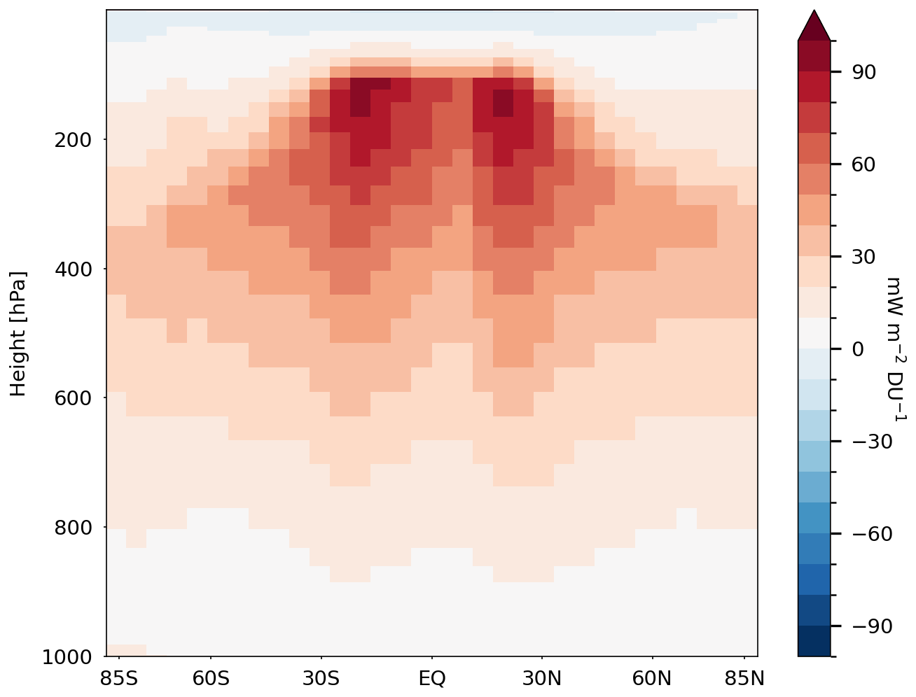
Figure 1 Radiative efficiencies (SARF) for ozone changes up to 0.1 hPa in mW m⁻² per DU based on calculations in Skeie et al. (2020).

RTMs themselves cannot calculate adjustments beyond stratospheric temperatures, but if the adjusted meteorological fields are provided from a GCM, a full ERF can be calculated. This technique is called a partial radiative perturbation (PRP) and was originally developed to analyse climate feedbacks (Colman and McAvaney, 1997) but has subsequently been used to analyse meteorological adjustments (Mülmenstädt et al., 2019; Smith et al., 2018). Not only can the PRP method be used to calculate a full ERF from an RTM, but if the meteorological changes are imposed one field at a time in the RTM, this method can decompose the total adjustment into each of its constituent components. Note that due to correlations between the meteorological changes (e.g. temperature and water vapour), the sum of the individual components is not equal to the total adjustments after applying the changes cumulatively (Coleman, 2024), although the residuum can be reduced by combining a forward and backward calculation for each component (Bickel et al., 2020; Colman and McAvaney, 1997; Klocke et al., 2013). As described above for the ozone changes, instead of running the RTM many times, it is possible to generate radiative kernels for each of the meteorological fields to generate 3D (or 2D for surface quantities) radiative sensitivities to changes in temperature, water vapour, cloud, albedo, etc. (Chung and Soden, 2015; Myhre et al., 2018; Pendergrass et al., 2018; Smith et al., 2018, 2020). These kernels can then be multiplied by the 3D (or 2D) meteorological changes to derive the adjustments. This kernel method will suffer from the same inability to account for correlations as the PRP.

Radiative forcing can also be calculated within GCMs or Earth system models (ESMs). The ERF is defined from Eq. (1) as the TOA imbalance when ΔT=0. There are two main methods for calculating this from ESMs. One method is to impose an abrupt forcing change in a simulation with a coupled ocean and then regress the TOA imbalance against surface temperature (regression method; Gregory et al., 2004). The ERF is then the TOA imbalance where the regression crosses ΔT=0. A second method is to fix the surface temperature in an atmosphere-only simulation (Hansen et al., 2005). Typically for practical model configuration reasons, only the sea surface temperature is fixed (fSST); however some studies have fixed the land surface temperature too (Ackerley and Dommenget, 2016; Andrews et al., 2021; Shine et al., 2003). In fSST simulations, the ERF needs to be corrected for any temperature change in the land surface (Tang et al., 2019). Both methods suffer from noise due to interannual variability. This is most pronounced in the regression method (Forster et al., 2016), making it unsuitable for quantifying the small forcings from changes in tropospheric ozone. The fSST method has less variability but still requires an integration of over 30 years to reduce the ERF uncertainty to below 0.1 W m⁻² (Forster et al., 2016). The internal variability in the fSST method can be reduced by constraining the winds to prescribed fields (nudging) (Kooperman et al., 2012). However, this can induce biases in the ERF (Coleman, 2024).

Components of the ERF can be diagnosed within the ESM fSST simulations through extra calls to the radiation scheme. Typically, these extra calls exclude clouds (“clear sky”), aerosols (“clean sky”) or both (“clear–clean sky”) (Ghan, 2013). The difference between “all sky” and “clear sky” or between “clean sky” and “clear–clean sky” can be used to quantify cloud adjustments. Note however that the “clear sky” or “clear–clean sky” ERF not only removes the cloud adjustments, but also removes the effects of cloud cover on the instantaneous radiative effect of ozone. The IRF for an ozone perturbation can be calculated within an ESM by including an additional diagnostic radiation call with a prescribed climatology of ozone (Dietmüller et al., 2016). The diagnostic radiation calls can be modified to include stratospheric-temperature adjustments (through FDH) and hence give online ESM calculations of SARF (Dietmüller et al., 2016; Stuber et al., 2001).

In this study we compare IRFs, SARFs and ERFs for ozone perturbations from offline kernel and online calculations to compare the consistency or otherwise of the methodologies and metrics.

2.3 Previous calculations of ozone radiative forcing

In this section, we review previous estimates of the pre-industrial to present-day ozone radiative forcing to highlight the diversity in estimates, which is driven by not only methodological diversity but also diversity in the time period of calculations. The separation between stratospheric ozone and tropospheric ozone forcing has been generally based on the vertical distribution of ozone rather than on the chemical drivers of the ozone change, i.e. ozone precursors or ODSs. This is particularly important in the stratosphere, where increases in lower-stratosphere ozone due to rising ozone precursor emissions have offset a significant fraction of the radiative forcing from historical ozone depletion (Shindell et al., 2013; Søvde et al., 2011).

The IPCC First Assessment Report (FAR) did not quantify the historical change in tropospheric ozone, but it did calculate radiative efficiencies for idealised ozone changes. This was 0.02 W m⁻² ppb⁻¹ based on Hansen et al. (1988), who used equilibrium temperature calculations from a 1D radiative–convective model. Subsequent reports (see Fig. 2 and Table S1) were based on historical ozone changes simulated in global atmospheric chemistry models with the radiative forcing calculated using offline RTMs. The dominant uncertainty in the historical forcing is the lack of knowledge of pre-industrial ozone precursor emissions (Stevenson et al., 2013) rather than uncertainty in the radiative forcing calculations or definitions.

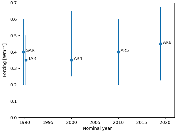
Figure 2 The tropospheric ozone radiative forcing from “pre-industrial” (1850 for SAR to AR4, 1750 for AR5 and AR6) to a nominal year assessed by the Second (SAR) to Sixth (AR6) IPCC Assessment Reports. Both SAR and the Third IPCC Assessment Report (TAR) used ozone concentrations representative of 1990 but have been offset in the figure for clarity. For data and references see Table S1.

Forcing from stratospheric ozone changes is sensitive to the altitude of the change, with decreases in lower-stratosphere ozone contributing a negative forcing and decreases in upper stratospheric ozone contributing a positive forcing (Skeie et al., 2020). Estimates of historical stratospheric ozone forcing have therefore been uncertain even in the sign. IPCC AR6 (Forster et al., 2021) references a forcing from historical stratospheric ozone changes of 0.02 ± 0.07 W m⁻² based on offline kernel SARF calculations in Skeie et al. (2020).

The ozone radiative forcing from historical ODS increases is more robustly negative as it excludes contributions from increasing ozone precursors and includes the impact of ozone depletion on upper-troposphere concentrations. IPCC AR5 (Myhre et al., 2013) quantified an ozone SARF attributed to ODSs of −0.15 ± 0.15 W m⁻² (where the uncertainty is a 5 %–95 % confidence limit), and AR6 (Szopa et al., 2021) found a value of −0.16 W m⁻² (no confidence limit provided). An ozone ERF of −0.04 ± 0.03 W m⁻² due to the historical ODS increase has been calculated from one model (Michou et al., 2020), but it is not clear that this can be directly compared to the SARF calculations.

3 Models and model simulations

3.1 Global models

The global models used in this study include a range of coupled chemistry–climate or Earth system models (CESM2, EMAC, GFDL-ESM4, GISS-E2.1, NorESM2 and UKESM1-0-LL) and the chemical transport model GEOS-Chem. Table 1 provides a summary of each model, and further model details are provided in the Supplement.

Table 1 List of the chemistry–climate, Earth system and chemical transport models used in this study, with details on the horizontal resolution, vertical levels and model lid, chemistry scheme, and relevant references.

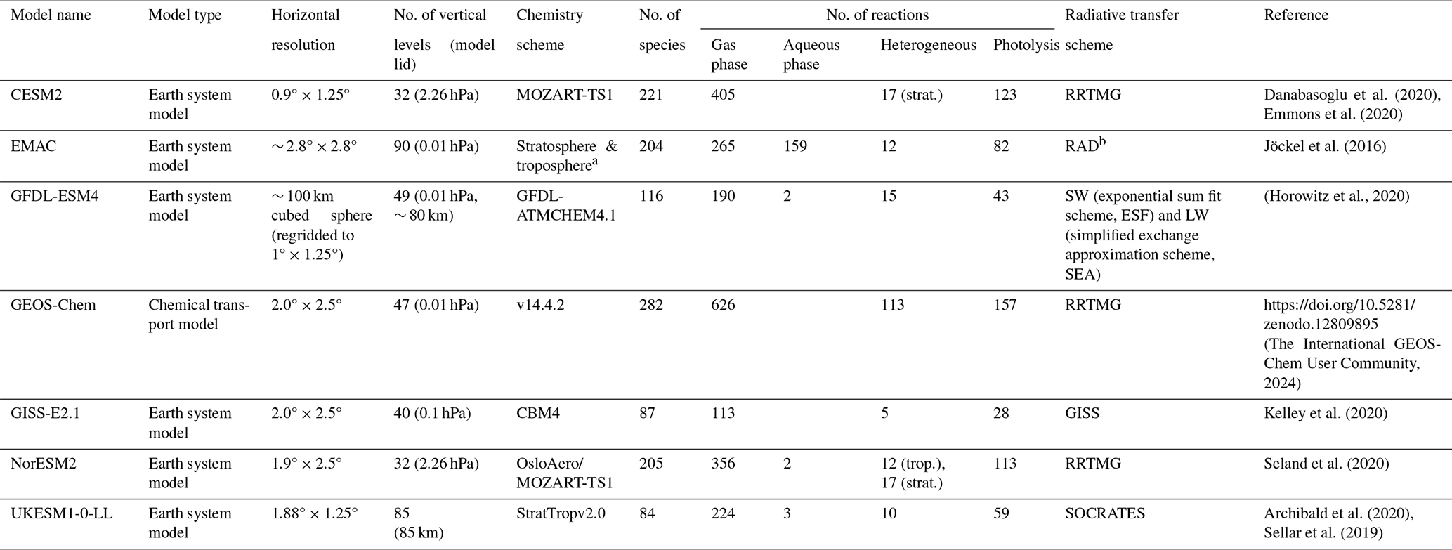
^a EMAC uses the submodel MECCA for gas-phase kinetics, the submodel SCAV for aqueous- and ice-phase kinetics and wet deposition, and the submodel MSBM for heterogeneous reaction rates on stratospheric aerosol and polar stratospheric clouds (see Supplement Sect. S1 for details). ^b EMAC uses the MESSy submodel RAD for radiative transfer calculations (see Supplement Sect. S1 for details).

3.2 Model simulations

The protocol for the model simulations carried out here is as follows.

As described in Sect. 2.2 and following recommendations from Forster et al. (2016) for the quantification of ERFs, the model simulations conducted here are atmosphere-only, with prescribed sea surface temperatures (SSTs) and sea ice cover (SIC). The control experiment (called pdClim-control) is a time-slice simulation for a continuous year, 2015, using prescribed climatologies for SSTs and SIC appropriate for the year 2015. Long-lived greenhouse gas concentrations for the year 2015, including those for ODSs, nitrous oxide and methane, are taken from the Shared Socioeconomic Pathway 3-7.0 (SSP3-7.0; Meinshausen et al., 2020). Other boundary conditions, such as ocean concentrations of dimethyl sulfide (DMS), are also prescribed by each model as climatologies appropriate for the present day. Emissions of non-methane ozone precursor gases, aerosols and aerosol precursors are prescribed as annually repeating emissions, using distributions and global annual totals from SSP3-7.0 for the year 2015, as prescribed for CMIP6 (Gidden et al., 2019). For those models that are free-running (prescribed SST/SIC), the control simulation was run for 50–70 years, allowing 30–40 years to be available for analysis following spin-up to reduce the effects of internal model variability. For those models that use specified dynamics (see below), the model control simulation was typically shorter in length following spin-up, i.e. 5–12 years in length. This was found to be sufficient for stabilisation.

The perturbation simulation (called pdClim-2050ssp370-radO3) is identical to that of the control, except that greenhouse gases including methane, nitrous oxide and ODS concentrations and all short-lived climate forcer emissions, as seen by the chemistry, are prescribed, using year-2050 values from SSP3-7.0. Although greenhouse gases, ozone precursors and aerosol emissions are perturbed here relative to the control, only perturbations to ozone itself can affect the top-of-atmosphere (TOA) radiative fluxes. The models' respective radiation and cloud microphysics schemes continue to see year-2015 atmospheric concentrations of greenhouse gases (GHGs), aerosols and cloud condensation nuclei, except for ozone. As a result, any difference in the TOA radiative fluxes between pdClim-control and pdClim-2050ssp370-radO3 is solely due to 2015-to-2050 changes in ozone (driven by changes in precursor emissions and ODSs and GHG concentrations) and any resulting rapid adjustments.

As the standard perturbation simulation also incorporates changes to ozone due to the expected reductions in ODSs (WMO, 2022), an additional perturbation simulation, pdClim-2050ssp370fODS-radO3, was performed by EMAC, CESM2, GFDL-ESM4 and UKESM1-0-LL. This additional perturbation simulation is identical to the standard perturbation simulation, pdClim-2050ssp370-radO3, except that ODSs were held at year-2015 values in the chemistry. Hence, this perturbation, which will be referred to as fODS-perturbation in the following, is designed to remove the effect of changing ODSs and connected changes in ozone. While the pdClim-2050ssp370-radO3 minus pdClim-2050ssp370fODS-radO3 ozone difference will be solely attributable to changes in ODSs, the focus of analysis will be on tropospheric differences between the fODS-perturbation and the present day (pdClim-2050ssp370fODS-radO3 minus  pdClim-control). Nitrous oxide (N₂O) may be an important factor with respect to ozone depletion in the 21st century, but the ozone response in the troposphere will be largely driven by changes in tropospheric ozone precursors in SSP3-7.0. To confirm this, one of the models (UKESM1-0-LL) performed an additional sensitivity simulation, in which both ODSs and N₂O were held at year-2015 values in the chemistry. A summary of the experimental setup for these 4 simulations can be found in Table 2, and Table 3 lists the length of spin-up and the number of years available for analysis from the participating models. In some cases, the protocol could not be implemented in a straightforward way. As a result, some bespoke model changes were made and are documented in the following paragraphs.

Table 2 List of the atmosphere-only (fSST) experiments carried out in this study to quantify year-2050 ozone effective radiative forcing relative to the year 2015 due to changes in well-mixed greenhouse gases (WMGHGs) and non-methane ozone precursors. VOCs denotes volatile organic compounds.

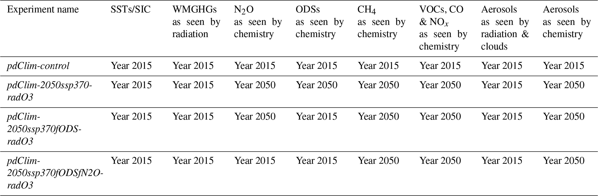
Table 3 List of participating global models in quantifying future ozone forcing. The table also includes the length of the model spin-up, the number of years available for analysis, and which ozone forcing calculations are available from the different models.

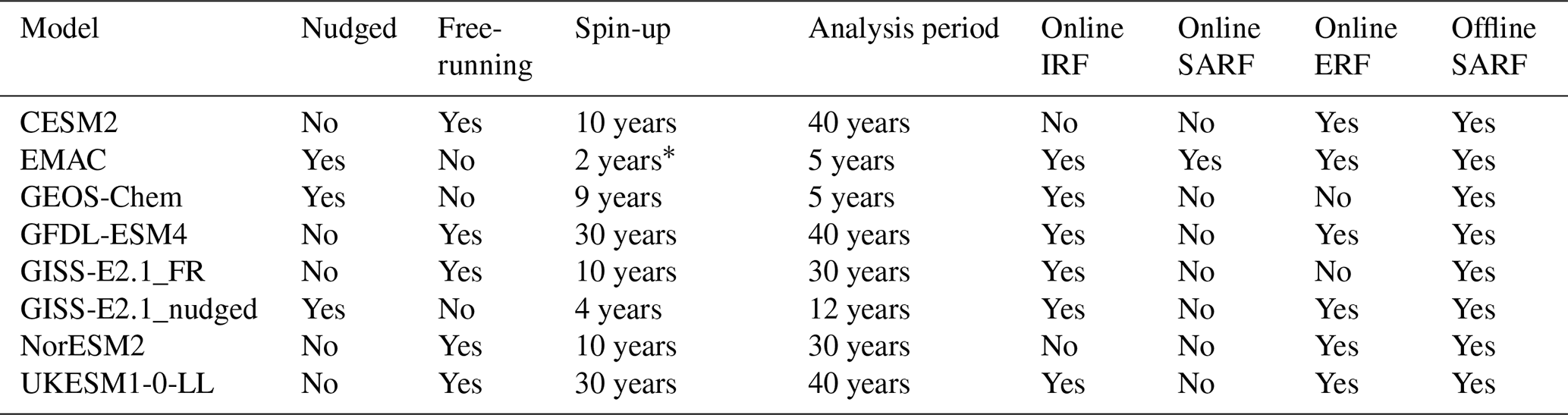
^* In the EMAC model, an additional spin-up of 10 years was undertaken in the pdClim-2050ssp370fODS-radO3 simulation.

In NorESM2 and CESM2, we were not able to implement the experimental protocol for the year-2050 perturbation simulation in all its aspects. For GHGs and ODSs, the model radiation scheme was successfully able to see GHGs/ODSs representative of 2015, while the model chemistry included GHGs/ODSs representative of the year 2050. However, this separation was not so feasible for both aerosols and methane-driven production of water vapour. In principle, in the perturbation simulation, the radiation and clouds (through microphysics) should see year-2015 aerosols, whereas the chemistry should see year-2050 aerosol surface densities for heterogeneous reactions.

Therefore, to obtain the ozone ERF in CESM2, we performed one further control experiment (called pdClim-control-fixO3) and one further perturbation experiment (called pdClim-2050ssp370fixO3-radO3). These are identical to CESM2's pdClim-control and pdClim-2050ssp370-radO3 in all aspects apart from the prescription of an O₃ climatology field that is seen only by the radiation scheme. In both cases, this climatology represents O₃ concentrations from the year 2010 as zonally averaged 5 d fields. As with pdClim-control and pdClim-2050ssp370-radO3, these additional experiments are run for 50 years, with the last 40 years used for analysis. Together, these simulations allow us to calculate the radiative and microphysical (cloud) impact of year-2050 aerosols and the radiative effect of CH₄-driven changes in stratospheric water vapour and to isolate the O₃ ERF by differencing the two experiment sets as (pdClim-2050ssp370-radO3 − pdClim-control) − (pdClim-2050ssp370fixO3-radO3 − pdClim-control-fixO3), as illustrated in Fig. S1 of the Supplement. Additionally, these simulations also allow us to isolate the tropospheric differences between CESM2's fODS-perturbation and the present day as (pdClim-2050ssp370fODS-radO3 − pdClim-control) − (pdClim-2050ssp370fixO3-radO3 − pdClim-control-fixO3).

A similar approach is used in NorESM2, whereby the 3D ozone climatology generated in pdClim-control and pdClim-2050ssp370-radO3 (from years 21–40) is used as input in two further simulations, R2 and P2, respectively. R2 is identical to NorESM2's pdClim-control in all aspects apart from the prescription of an O₃ climatology field that is seen only by the radiation scheme that is representative of O₃ distribution for the year 2015. Likewise, P2 is identical to pdClim-control apart from the prescription of O₃ climatology representative of the year 2050. Differencing P2 and R2 then allows us to isolate the O₃ ERF in NorESM2.

In EMAC, we use nudging or “specified dynamics”, i.e. Newtonian relaxation towards ERA5 data (Hersbach et al., 2020), so that the reference and the perturbation simulation have the same meteorology. The relaxation is applied in spectral space for the prognostic variables of divergence, vorticity, temperature, and (logarithm of the) surface pressure. The mean temperature (i.e. wave zero) is not nudged (see Jöckel et al., 2016, for more details). Therefore, only 5 simulation years is necessary for the analyses. Furthermore, we use a slight variation of the “quasi chemistry-transport model mode” described by Deckert et al. (2011). This mode enables a decoupling of dynamics and chemistry. For this we performed one simulation with full coupling of dynamics and chemistry but otherwise the same setup as the pdClim-control simulation (called pre). The setup uses prescribed climatologies for tropospheric and stratospheric aerosol for the radiation calculation and for the heterogeneous chemistry on particle surfaces. The aerosol climatologies used for heterogeneous chemistry stem from the model simulations described by Righi et al. (2023), with different climatologies for the 2015 simulation (SSP2-4.5) and the 2050 simulations (SSP3-7.0). For the radiation calculation in the pdClim-control, pdClim-2050ssp370-radO3 and pdClim-2050ssp370fODS-radO3 simulations from EMAC, all radiative active trace gases, except for ozone and water vapour, are then prescribed from monthly mean transient files from this pre simulation. Moreover, we used monthly mean OH values from this simulation with the CH₄ lower boundary condition from pdClim-control for a parameterised methane oxidation scheme as a source for stratospheric water vapour in all simulations via the CH₄ submodel (Winterstein and Jöckel, 2021).

In GFDL-ESM4, the chemical production of water vapour, including from the oxidation of methane and hydrogen, is disabled and replaced by nudging stratospheric water vapour to an analytic approximation of the climatology retrieved by the HALogen Occultation Experiment (HALOE), as described by Harris et al. (2021). The aerosol concentrations used in the radiation and aerosol activation schemes are prescribed externally and are identical in the control and perturbation simulations. The aerosol concentrations used were scaled from the aerosol concentration forcing fields provided for CMIP5, rescaled globally to approximately match the global mean aerosol optical depths and burdens simulated by GFDL-ESM4. In addition, the ability to add an additional diagnostic radiative transfer call with ozone set to zero throughout the atmosphere was added to GFDL-ESM4 to allow calculations of ozone's direct radiative effect.

Two sets of simulations were carried out with the GISS-E2.1 model – free-running (FR) and nudged. No additional bespoke changes were made to the GISS-E2.1 FR simulations, denoted as GISS-E2.1_FR hereafter. In GISS-E2.1 with nudging – called GISS-E2.1_nudged hereafter – horizontal winds only were nudged towards the year 2015 of a MERRA2 3-hourly dataset (Gelaro et al., 2017), and the simulations were run for more years than for the EMAC nudged model (Table 3). For the control simulation, SSP2-4.5 2015 emissions were used, though Shared Socioeconomic Pathway emissions were similar among pathways for this year, as they were harmonised to meet historical emissions in 2015 (Gidden et al., 2019). The perturbation simulation used SSP3-7.0 year-2050 emissions. Sea surface conditions and vegetation were prescribed as 2015 values, as prepared for CMIP6 (Kelley et al., 2020), rather than as a climatology. A few alterations were made to the model code to conform closely to the protocol. With standard code, the radiative transfer calculation experiences chemical ozone changes without experiencing methane or aerosol changes. However, the chemical change to water vapour reaching the radiation code is normally changed in unison with ozone. In the simulations here, this was decoupled such that the water vapour changes due to chemistry did not affect the radiation. An alteration was also needed to allow the perturbation simulation to use year-2050 greenhouse gases (CH₄, CFCs, N₂O) in the chemistry while maintaining year-2015 values in the radiation calculations.

In UKESM1-0-LL, stratospheric water vapour production from methane oxidation, as documented in Archibald et al. (2020), was deactivated. In its place, a parameterisation for methane oxidation independent of the chemistry scheme was activated, in which the methane mixing ratio was implicit and derived from the assumption that 2 [CH₄] + [H₂O] = 3.75 ppm throughout the stratosphere. In this way, from a radiative perspective, stratospheric water vapour in pdClim-control and pdClim-2050ssp370-radO3 was set close to a value of 3.75 ppm. In addition, an extra diagnostic call to the SOCRATES radiative transfer scheme with ozone set to a prescribed climatology was added to allow the calculation of ozone's direct radiative effect.

3.3 Online double radiation calls for ozone

In addition to the diagnosis of TOA radiative fluxes for the purpose of quantifying ERF, some models included a diagnostic call to the radiation scheme with a reference ozone field. Analogously to the Ghan (2013) method for aerosols, differences between radiative fluxes from the diagnostic and prognostic radiation calls between the control and perturbation experiments enable an ozone IRF to be calculated. In some models (e.g. EMAC), the diagnostic call included a stratospheric-temperature difference relative to the prognostic call; in this case, an ozone SARF can be calculated. In other models (e.g. GEOS-Chem), the online double radiation call for ozone was the only online means of diagnosing an ozone forcing metric. Table 3 lists which models included online double radiation calls for ozone and for which metric.

3.4 Offline ozone radiative kernel method

To calculate TOA SARF, a top-of-atmosphere version of the radiative kernel for stratospheric-temperature adjusted radiative forcing (SARF) at the tropopause (Skeie et al., 2020) is used. The monthly mean ozone mixing ratios in pdClim-ssp370-radO3 and pdClim-control are regridded horizontally and vertically to the resolution of the radiative kernel (T21 (∼ 5.6° at the Equator) and 60 vertical levels from the surface and up to 0.1 hPa). The radiative kernels are monthly 3-dimensional fields of RF at the top of atmosphere per DU change for SW (clear sky, all sky), LW (clear sky, all sky) and LW (all sky) including stratospheric-temperature adjustments (Fig. S2). Net SARF is calculated as the sum of SW all sky and LW all sky adjusted. For comparison with the online IRF calculations, the IRF kernel is the sum of SW and LW for either clear sky or all sky. For each year in the model simulations, the kernel is multiplied by the difference in ozone mole fractions between the two experiments converted to DU using common meteorological fields native to the radiative kernel.

In addition to the calculation of TOA SARF for the total ozone changes, separate calculations are also performed for tropospheric ozone changes, where the tropopause is defined for each month based on the ozone mole fraction (<150 nmol mol⁻¹) in pdClim-control.

4 Results

4.1 Modelled ozone changes

From the experimental setup described above, year-2015 and year-2050 ensemble-mean climatologies for total column ozone (TCO) are shown in Fig. 3, with results from the individual models shown in Fig. S3 of the Supplement. For the present day and based on 7 of the 8 participating models, the multi-model global mean TCO is 298.3 ± 8.3 DU, with minimum values in the tropics and southern high latitudes and maximum values in the northern middle to high latitudes. Following SSP3-7.0, global mean TCO increases to 310.5 ± 10.4 DU in 2050 in the ensemble mean, with the largest increase occurring in the southern high latitudes. From a multi-model perspective, this represents a global mean TCO increase of 12.2 ± 5.2 DU in response to reduced ODSs combined with increases in nitrous oxide, carbon dioxide, methane and non-methane ozone precursors. Looking at the individual model responses, the increase in global mean TCO is in the range of 2.1 DU (GISS-E2.1_nudged) to 19.6 DU (UKESM1-0-LL). Most models also show increases in TCO in all regions of the globe. While GISS-E2.1_nudged shows a weak increase in global mean TCO in 2050 (Fig. S3), decreases in the northern high latitudes and particularly in the southern high latitudes are evident. This anomalous response may be due to that model's implementation of nudging (Orbe et al., 2020) and is contrary to the scientific understanding of stratospheric ozone recovery and CMIP6 projections (Keeble et al., 2021). As a result, GISS-E2.1_nudged was omitted from the ensemble mean in Fig. 3 and all ensemble means hereafter. This 7-model ensemble is hereafter referred to as the TOAR-RF ensemble. The range for the increase in global mean TCO from the remaining models is 4.3–19.6 DU and is shown in Table 4.

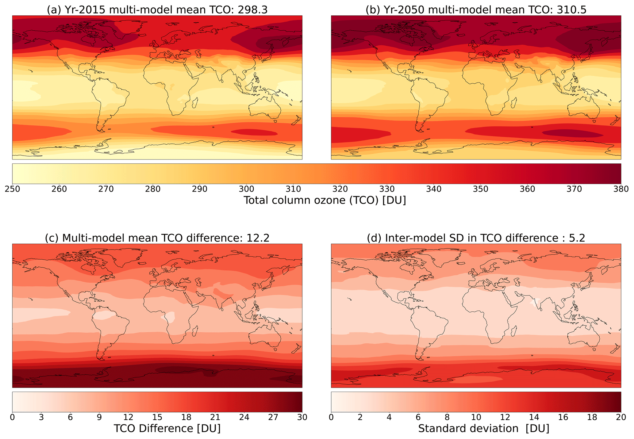
Figure 3 Multi-model mean climatologies of total column ozone (TCO) in Dobson units (DU) for (a) the present day (year 2015) and (b) the future (year 2050) following the SSP3-7.0 scenario, (c) the multi-model mean difference between the climatologies (year 2050 minus year 2015), and (d) the inter-model standard deviation about the multi-model mean difference. Models included in the multi-model means are CESM2, EMAC, GEOS-Chem, GFDL-ESM4, GISS-E2.1_FR, NorESM2 and UKESM1-0-LL. Global ensemble mean values are shown above each panel.

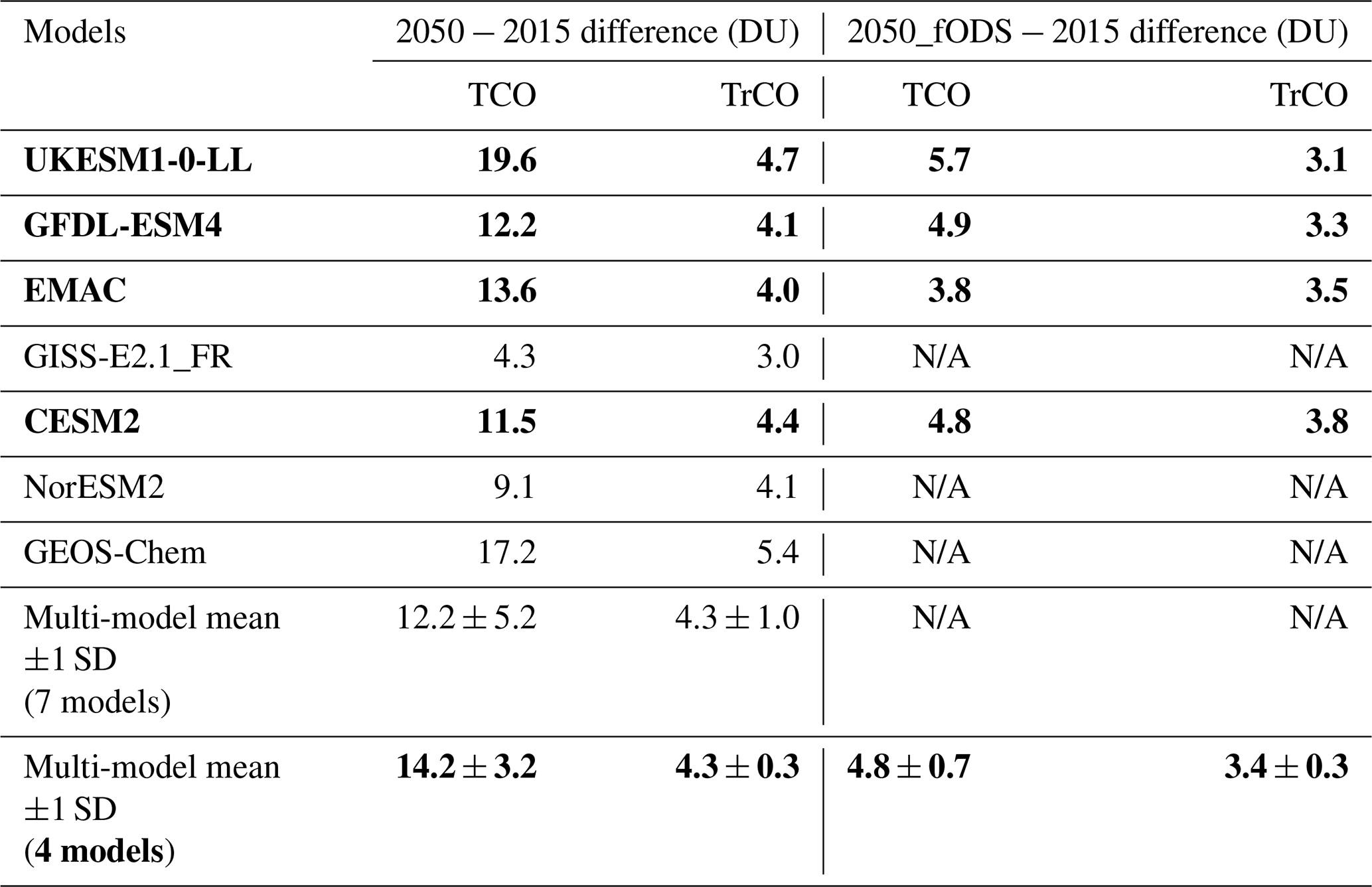
Table 4 Differences in global multi-annual mean total column ozone (TCO) and tropospheric column ozone (TrCO) in Dobson units (DU) between 2015 and 2050 for pdClim-2050ssp370-radO3 relative to pdClim-control from the 7 members of the TOAR-RF ensemble and for pdClim-2050ssp370fODS-radO3 relative to pdClim-control from the 4 models that ran the sensitivity simulation (in bold). Multi-model means and standard deviations are shown for the 7-member and 4-member ensembles. N/A indicates where data are not available.

Using the definition of the tropopause based on the ozone mole fraction (<150 nmol mol⁻¹) in pdClim-control and the same 7-member ensemble as for TCO, year-2015 and year-2050 climatologies for tropospheric column ozone (TrCO) from the ensemble mean and from all of the individual models are shown in Figs. 4 and S4, respectively. In 2015, TrCO shows multi-model global mean values of 36.2 ± 1.1 DU, with maximum values in the sub-tropics and northern mid-latitudes and minimum tropospheric column amounts over the tropical Pacific and southern high latitudes. Following SSP3-7.0, the multi-model global mean TrCO increases to 40.5 ± 1.1 DU in 2050, representing a multi-model global mean increase of 4.3 ± 1.0 DU (Table 4). This indicates that of the TCO changes shown in Fig. 3 and Table 4, 39 ± 14 % of the increase occurs within the troposphere. Regionally, the largest increase in TrCO occurs over the Middle East, India and southeast Asia and the largest inter-model spread in the TrCO increase is in the southern high latitudes. Looking at the individual models, present-day global mean TrCO ranges from 35.0 DU in GFDL-ESM4 to 39.7 DU in GISS-E2.1_nudged. While most models broadly agree on the spatial distribution in the present day, maximum column amounts extend further into the northern high latitudes in the GISS-E2.1 model simulations, and they also show the deepest minimum over the tropical Pacific. In 2050, following SSP3-7.0, TrCO increases globally in all models, with global mean values in the range of 39.1–42.2 DU. However, the increases are more regionally confined to the Northern Hemisphere sub-tropics in the GISS-E2.1 model simulations, whereas the other models show that substantial increases also occur elsewhere (e.g. high latitudes) in response to the changes in well-mixed greenhouse gases and ozone precursors in SSP3-7.0.

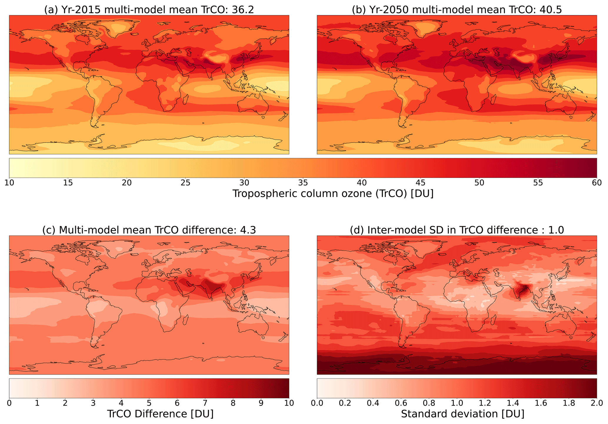
Figure 4 Multi-model mean climatologies of tropospheric column ozone (TrCO) in Dobson units (DU) for (a) present-day (year-2015) and (b) future (year 2050) global distributions, (c) the multi-model mean difference between the climatologies (year 2050 minus year 2015), and (d) the inter-model standard deviation about the multi-model mean difference. Models included in the multi-model means are the same as in Fig. 3. Global ensemble mean values are shown above each panel.

Figure 5 shows the TOAR-RF 7-member ensemble-mean zonal-mean ozone climatology for the present-day (year 2015) and future (year 2050), along with the difference between them. Climatologies for each individual model are shown in Fig. S5. In the 7-model ensemble mean, future zonal-mean ozone increases almost everywhere from present-day values following SSP3-7.0. The only exception to this is in the tropical and Northern Hemisphere stratosphere, centred around 10 hPa, where a reduction in zonal-mean ozone of less than 1 % occurs. The largest increase occurs in the southern high latitudes between 60 and 90° S and 300–80 hPa, where zonal-mean increases of greater than 20 % are evident. However, the variability in the modelled response in this region also reaches a maximum, with the inter-model standard deviation in the zonal-mean relative difference being greater than 10 %. In the troposphere, zonal-mean ozone increases in all regions in 2050. Increases in tropospheric ozone precursors drive increases of up to 14 %, with the largest increase occurring through the depth of the troposphere in the Northern Hemisphere tropics and sub-tropics. The inter-model standard deviation in the tropospheric zonal-mean ozone increase is typically between 2 % and 4 %.

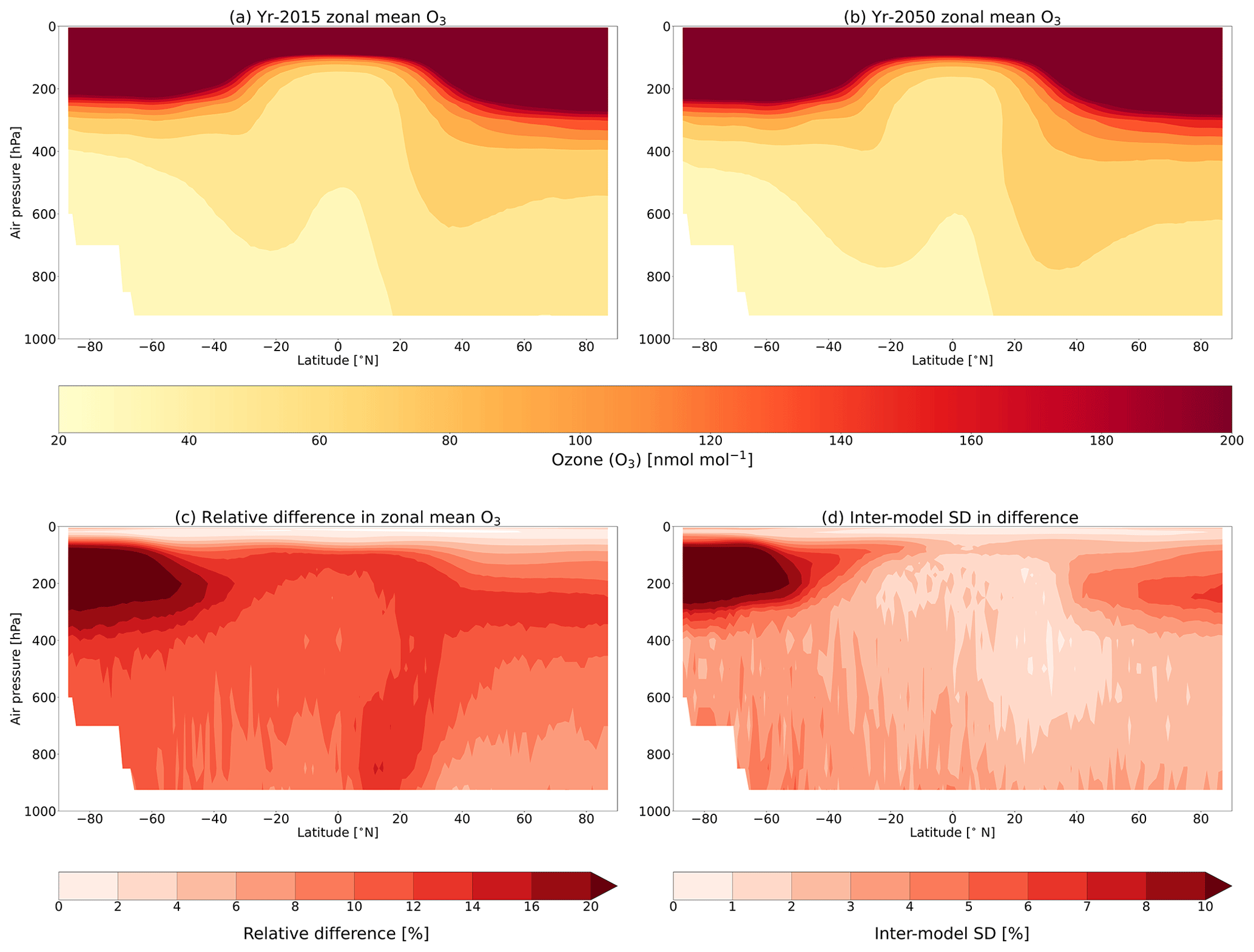
Figure 5 Multi-model zonal-mean climatologies of (a) present-day (year 2015) and (b) future (year 2050) ozone distributions, (c) the multi-model mean relative difference between the climatologies (year 2050 minus year 2015), and (d) the inter-model standard deviation about the multi-model mean relative difference. Units of ozone are in nmol mol⁻¹ in panels (a) and (b). Models included in the multi-model means are CESM2, EMAC, GEOS-Chem, GFDL-ESM4, GISS-E2.1_FR, NorESM2 and UKESM1-0-LL.

Looking at the individual model zonal-mean climatologies and responses (Fig. S5), the models indicate that the largest relative changes occur in the southern high-latitude upper troposphere and lower stratosphere. Apart from the GISS-E2.1_nudged simulation, there are weaker positive and negative changes aloft and there is evidence of secondary peak increases in the extra-tropical stratosphere (between 1 and 10 hPa) for those models with a higher model lid. Although GISS-E2.1_nudged shows the strongest increases in this region, the negative TCO changes in the future (Fig. S3) result from reductions in ozone of 5 %–30 % throughout the lower stratosphere, with the largest reductions occurring in the southern high latitudes.

4.2 Ozone evaluation

As a result of the bespoke changes made to the different models to meet the requirements of the experimental protocol, it is important to assess any potential impact they may have had on model performance. As a result, modelled ozone is benchmarked against CMIP6 historical and future SSP3-7.0 simulations and observations, where available. Figure 6 shows a comparison of modelled TCO between 60° S and 60° N from the pdClim-control and pdClim2050ssp370-radO3 simulations against the CMIP6 ensemble and observations (Bodeker et al., 2021). It shows that the present-day (year 2015) TOAR-RF ensemble-mean TCO of 294.5 ± 9.5 DU is in excellent agreement with that from CMIP6 (297.5 ± 12.7 DU; Keeble et al., 2021). The historical trend in CMIP6 ozone agrees well with that observed; however, both the CMIP6 ensemble mean and the TOAR-RF ensemble mean are systematically biased high relative to observations (283.5 ± 1.1 DU) by approximately 10 DU. In 2050, the TOAR-RF area-weighted TCO ensemble mean is projected to increase to 305.2 ± 12.3 DU following SSP3-7.0 and is again consistent with that from the CMIP6 ensemble (308.5 ± 11.8 DU; Keeble et al., 2021). This suggests that the bespoke changes did not have a negative impact on modelled TCO performance relative to CMIP6, although the CMIP6 ensemble includes changes in climate which are excluded in the TOAR-RF simulations.

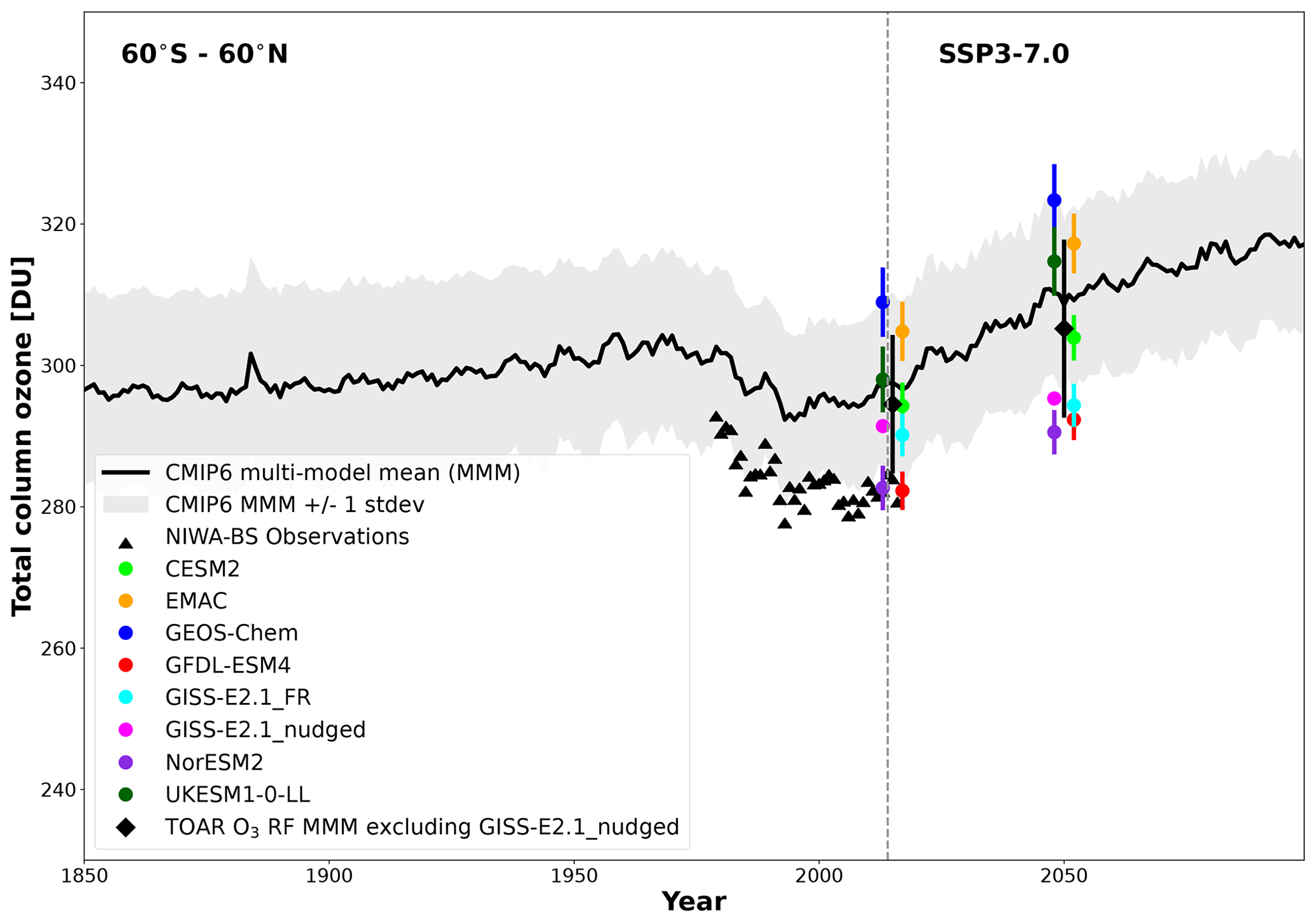
Figure 6 Comparison of the climatological total column ozone (TCO) averaged over 60° S–60° N and its variability expressed as ±1 standard deviation from the time-slice simulations for the years 2015 and 2050 from all of the individual models (CESM2 in light green; EMAC in orange; GEOS-Chem in blue; GFDL-ESM4 in red; GISS-E2.1_FR in light blue; GISS-E2.1_nudged in magenta; NorESM2 in purple and UKESM1-0-LL in dark green) in comparison with the CMIP6 multi-model mean (solid black line) and ±1 standard deviation (grey shading) from coupled transient historical and future simulations using SSP3-7.0, including historical observations from NIWA-BS (black triangles). Individual model results are slightly offset from 2015 and 2050 for greater clarity. The TOAR-RF multi-model mean (black diamond) and the inter-model spread expressed as ±1 standard deviation from this study is based on the following models: CESM2, EMAC, GEOS-Chem, GFDL-ESM4, GISS-E2.1_FR, NorESM2 and UKESM1-0-LL. Figure adapted from Keeble et al. (2021).

In terms of individual model performance, present-day TCO from NorESM2 (282.7 ± 2.8 DU) and GFDL-ESM4 (282.3 ± 2.4 DU) sits just outside the lower edge of the ±1 standard deviation CMIP6 multi-model envelope, indicating that both models are in excellent agreement with the observations (283.5 ± 1.1 DU from the 2010–2014 time period; Bodeker et al., 2021). At the other end of the TOAR-RF ensemble, GEOS-Chem has the highest present-day TCO values of 308.9 ± 4.6 DU, with a systematic bias of more than 25 DU with respect to the observations. However, it is still within the ±1 standard deviation of the CMIP6 multi-model ensemble. It is also worth noting that modelled TCO from StratTropv2.0 in UKESM1-0-LL is well within the inter-model spread of the CMIP6 and the TOAR-RF ensembles, whereas TCO from StratTropv1.0 was biased high relative to both CMIP6 and observations (Keeble et al., 2021).

4.3 Online radiative forcing

Here we intercompare the ozone forcing metrics calculated online by the global models. Figure 7 shows the global mean online-calculated IRF, SARF and ERF corresponding to changes between the simulations pdClim-2050ssp370-radO3 and pdClim-control. Results of the GISS-E2.1_nudged model are excluded in Fig. 7 and in the following description, as in Sect. 4.1.

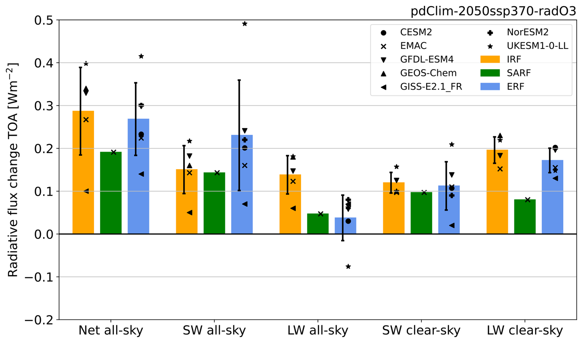
Figure 7 Online-calculated IRF, SARF and ERF corresponding to the standard perturbation pdClim-2050ssp370-radO3 minus pdClim-control (2050–2015). The multi-model means are represented by the coloured bars. Note that there is a variation in the number of models that provided each diagnostic. SARF was only provided by the EMAC model. The multi-model spread is given by the inter-model standard deviation. The markers represent individual model estimates.

The multi-model mean ERF and IRF are 0.268 ± 0.084 W m⁻² (6 models) and 0.288 ± 0.101 W m⁻² (5 models), respectively (see Tables S2 and S4). All models, except for GISS-E2.1_FR, indicate a significant positive ERF (see Table S4). Similarly, all models indicate a significant positive IRF (see Table S2). Individual models do not agree whether rapid adjustments enhance or reduce the ERF, as for some models ERF is greater than IRF (GISS-E2.1_FR, UKEMS1-0-LL), whereas for others ERF is smaller than IRF (EMAC, GFDL-ESM4). The partitioning between LW and SW radiative forcing changes from IRF to ERF. The multi-model mean SW all-sky ERF is enhanced compared to SW IRF, whereas the LW all-sky ERF is reduced compared to LW IRF. Also, the individual models agree that the SW all-sky ERF is reduced in comparison to SW all-sky IRF.

SARF was calculated as an online diagnostic only by EMAC, indicating a SARF of 0.191 ± 0.003 W m⁻² (see Table S3). The SARF is reduced by 0.076 W m⁻² compared to the IRF.

The spatial distribution of online-calculated all-sky and clear-sky ERF, IRF and SARF from the EMAC model simulation is shown in Fig. S6. The EMAC model was used as it is the only model that provides all the online diagnostics, and we wanted to ensure a fair comparison of the spatial distributions across the metrics by using the same model throughout. Except for the all-sky ERF, all other forcing diagnostics show positive flux changes throughout the globe in EMAC. For all-sky ERF, the fluxes show considerable noise due to cloud changes between the simulations (see Sect. 4.5). This demonstrates that even with nudging there is large variability in cloudiness. The largest values of ERF and IRF (both clear-sky and all-sky) can be found in the Southern Hemisphere polar region (Fig. S6a), related to changing ODS abundances in the two simulations (see Sect. 4.7 for details). For SARF, the high southern-latitude forcing is much reduced by the stratospheric-temperature adjustment and the largest flux changes are found in the Northern Hemisphere at around 25° N. Local maxima of IRF/SARF (both clear-sky and all-sky) and clear-sky ERF can be found over northern Africa, the Arabian Peninsula and the northern part of the Indian subcontinent, resembling the largest changes in tropospheric column ozone found in these regions and shown in Figs. 4c and S4.

In summary, the net all-sky multi-model mean ERF is similar to the IRF within the uncertainties due to a reduction in the LW forcing but an increase in the SW forcing. The ERF is higher than the SARF for the one model that calculated it, particularly in the clear sky.

4.4 Offline radiative forcing

The SARF at TOA from the ozone changes between pdClim-2050ssp370-radO3 and pdClim-control is calculated offline using the radiative kernel (see Sect. 3.4). The results are shown in Fig. 8, where contributions from total ozone radiative forcing are shown as coloured bars, and the tropospheric forcing is indicated by hatching. The SARF for total ozone ranges from 0.134 to 0.319 W m⁻² (Table S5) with 57 % to 93 % contribution from ozone in the troposphere ranging from 0.125 to 0.186 W m⁻² (Table S6). The multi-model mean SARF is 0.244 ± 0.057 W m⁻² for total ozone and 0.155 ± 0.019 W m⁻² for tropospheric ozone. The multi-model mean includes GEOS-Chem; excluding this model for comparison with the ERF in Sect. 4.3 gives 0.233 ± 0.046 W m⁻².

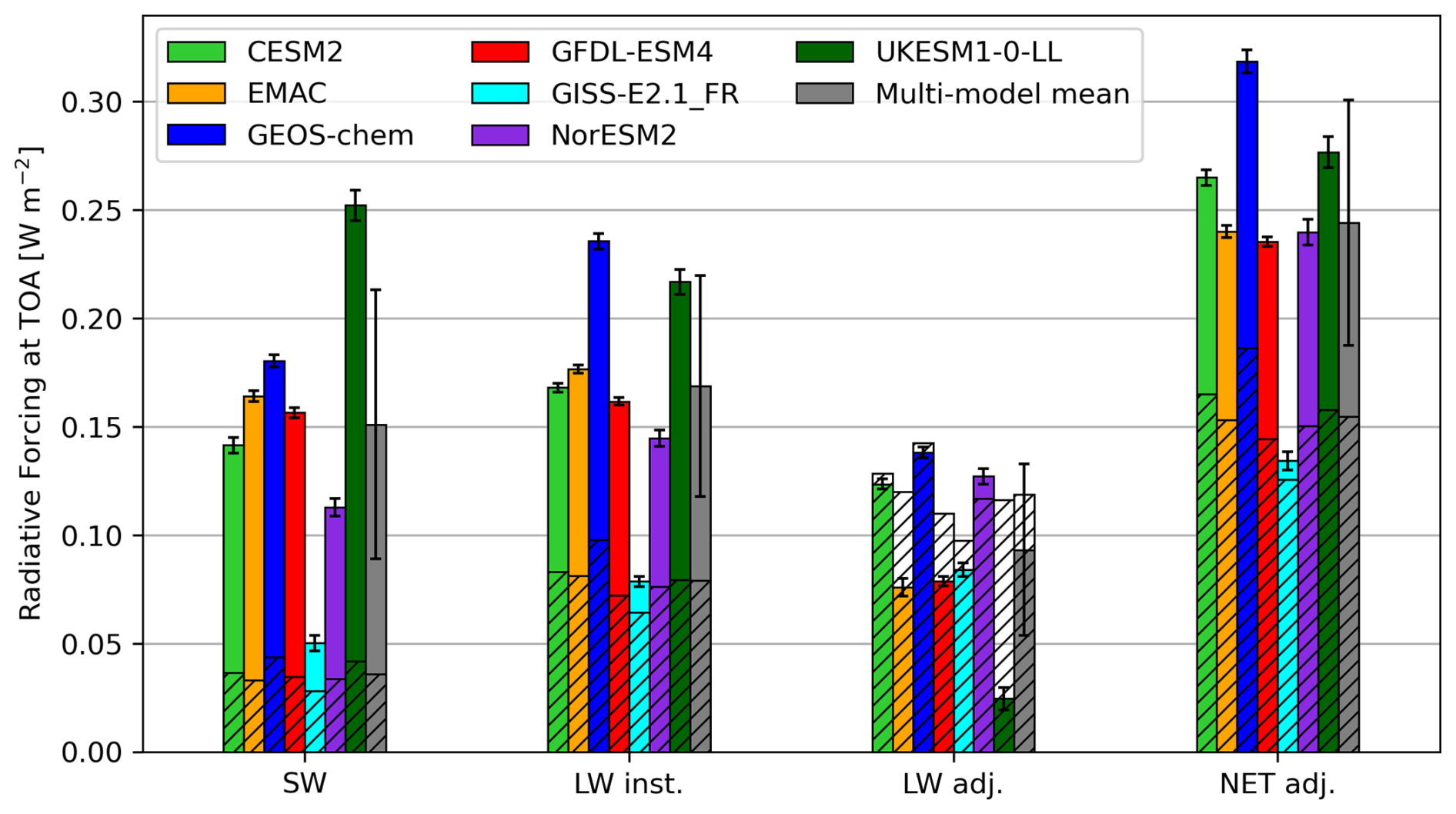
Figure 8 The radiative forcing at TOA calculated offline using the radiative kernel. The results are separated for short wave (SW), long wave instantaneous (LW inst.), long wave including stratospheric-temperature adjustments (LW adj.) and the net SARF (NET adj.) The total ozone forcing for the individual models is shown as a coloured bar, and the corresponding standard error is indicated by the error bar. The multi-model means are shown as grey bars to the right, where the error bars indicate the standard deviation of the multi-model spread. The hatched parts of the bars are the contribution from the tropospheric ozone changes, where the tropopause is defined by a 150 nmol mol⁻¹ ozone mole fraction in the pdClim-control simulations.

The TOA SARF is dependent on the latitude and altitude of the ozone change (Fig. S2f), and these dependencies come mainly from the LW (Fig. S2e). For the SW radiative forcing, there are fewer dependencies on latitude and altitude (Fig. S2b), and the SW RF, including the split between tropospheric and stratospheric contributions, reflects changes in the ozone burden (Figs. S3 and S4). For the LW adjusted radiative forcing, the magnitude is dependent on where ozone changes occur. The increase in stratospheric ozone in the models contributes to a negative LW adjusted radiative forcing, so the total LW adjusted radiative forcing is less than the tropospheric contribution except for NorESM2 (Fig. 8).

There is close agreement between models in the tropospheric forcing but with more model variability when including stratospheric changes, as indicated by the large standard deviation across models in the total ozone radiative forcing.

4.5 Cloud changes

The ERF from the ozone perturbation includes adjustments due to changes in clouds. To study this in more detail, we focus on global vertical profiles of ozone, temperature, cloud fraction, humidity, cloud cover and TOA radiative fluxes. We exclude GISS-E2.1_nudged from this analysis, as it shows rather different ozone and cloud responses, and GEOS-Chem, which as a chemical transport model (CTM) does not allow for cloud changes. The top row of Fig. 9 shows the difference in the global mean profile of ozone, temperature, cloud fraction and humidity between the pdClim-2050ssp370-radO3 and pdClim-control simulations. The difference in ozone (shown for 6 of the models in Fig. 9a and b) is mostly positive and strongest above 200 hPa (when expressed as a mole fraction). All six models shown here are in reasonable agreement, except for GISS-E2.1_FR, which shows only a weak stratospheric signal. In the troposphere, all models indicate an increase in ozone (which is more visible when expressed in partial pressure in Fig. 9b), with GISS-E2.1_FR showing a weaker response than the other 5 models. The difference in temperature between both simulations (shown in Fig. 9c) is most pronounced and positive between 300 and 50 hPa and negative above 50 to 20 hPa. The vertical profile of the cloud fraction (shown in Fig. 9d) generally shows a decrease, and this signature is strongest between 400 and 100 hPa. Some models show a secondary peak in the reduction of the cloud fraction at around 800 hPa (CESM2, NorESM2 and UKESM1-0-LL), although other models do not. EMAC (orange line) shows a relatively weak difference for temperature and cloud fraction, reflecting the effect of nudging on limiting the response in this model. The vertical profile of relative change in humidity (expressed as a % change in specific humidity, shown in Fig. 9e) shows a maximum increase of 3 % to 5 % in the stratosphere around 100 hPa. In the troposphere, the change is smaller and increases with height from the surface to the tropopause. The change in the stratosphere humidity is due to meteorological adjustments, such as through higher tropospheric humidity and higher tropical upper-troposphere–lower-stratosphere (UTLS) temperature, rather than chemical adjustments. The experimental setup was designed to have similar chemical water vapour production from methane oxidation in all simulations.

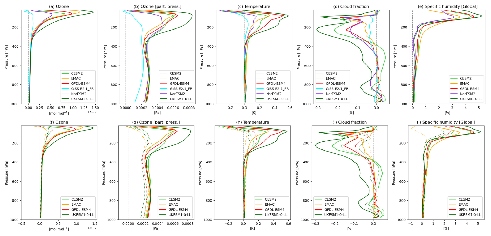
Figure 9 Global mean profile of difference in (a, f) ozone mole fraction, (b, g) ozone partial pressure (Pa), (c, h) temperature (K) and (d, i) cloud fraction (%) and of relative difference (e, j) in specific humidity between the 2050 and 2015 (pdClim-control) state. Panels (a)–(e) show the results from the standard experiment pdClim-ssp2050ssp370-radO3 minus pdClim-control; panels (f)–(j) show for the models that ran the fODS-perturbation experiment (CESM2, EMAC, GFDL-ESM4, UKESM1-0-LL). The results from the standard (pdClim-ssp2050ssp370-radO3 minus pdClim-control) experiment are shown using solid lines (which are repeated from panels a–e), and fODS (pdClim-ssp2050ssp370fODS-radO3 minus pdClim-control) experiments are shown using dotted lines.

The bottom row in Fig. 9 (panels f, g, h, i, j) shows results for the sensitivity experiment pdClim-2050ssp370fODS-radO3 (see Sect. 4.7) using dotted lines. For the four models that performed the pdClim-2050ssp370fODS-radO3 experiment (CESM2, EMAC, GFDL-ESM4 and UKESM1-0-LL), we find a weaker but still coherent response in the vertical profiles of these variables.

The impact seen in the vertical profile of the cloud fraction can also be observed in the change in the total cloud cover, which is an integrated value over the whole atmospheric column. Table 5 gives the global mean cloud cover in the reference simulation pdClim-control (in the second column) and the difference between pdClim-2050ssp370-radO3 and pdClim-control (third column) for the different models. UKESM1-0-LL shows the strongest reduction in cloud cover, followed by slightly weaker responses in NorESM2, CESM2 and GFDL-ESM4 and a relatively small response in EMAC. The cloud cover response for GISS-E2.1_nudged is also listed in Table 5 but is not further used in the analysis. Table 5 also shows the contribution of clouds to the TOA SW and LW ERFs. These values have been obtained as the difference between the all-sky (AS) and clear-sky (CS) TOA ERFs, which will also include the effects of cloud masking. Figure 10 shows this cloud contribution to the TOA ERFs as a function of the change in cloud cover. For the SW ERF (Fig. 10a) we find a clear negative relationship, and we find a positive relationship in the LW ERF (Fig. 10b). Figure 10c shows the net (SW + LW) contribution of clouds to the TOA ERF. It is the difference between two relatively large numbers and shows little correlation with the cloud cover change. Figure 10 contains the impacts both of the standard experiment pdClim-2050ssp370-radO3 (circles) and of the sensitivity experiment pdClim-2050ssp370fODS-radO3 (triangles). The pdClim-2050ssp370fODS-radO3 experiment is more deeply discussed in Sect. 4.7.

Table 5 Global mean cloud cover in the reference simulation (pdClim-control); absolute difference in cloud cover between both simulations (pdClim-2050ssp370-radO3 minus pdClim-control); and contribution of clouds to the SW, LW and net ERF. The uncertainty for the individual models is the error of the mean. The multi-model mean is calculated using 6 models: CESM2 (average of the two members), EMAC, GFDL-ESM4, GISS-E2.1_FR, NorESM2 and UKESM1-0-LL. The uncertainty in the multi-model mean is the standard deviation between the models.

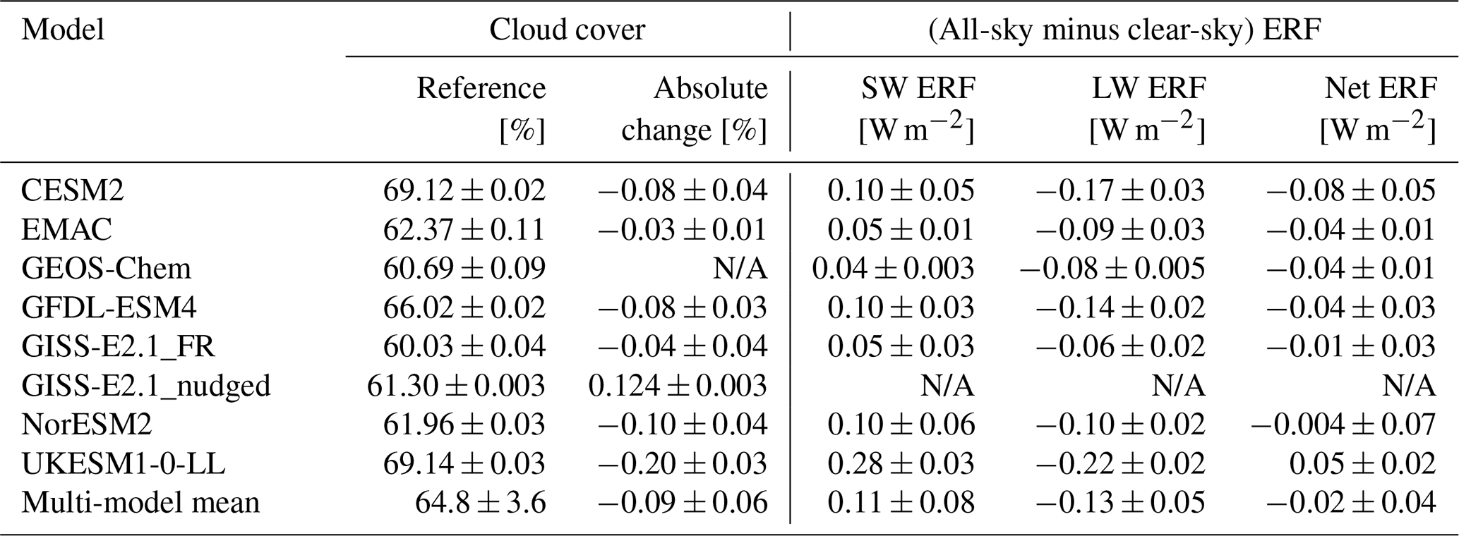
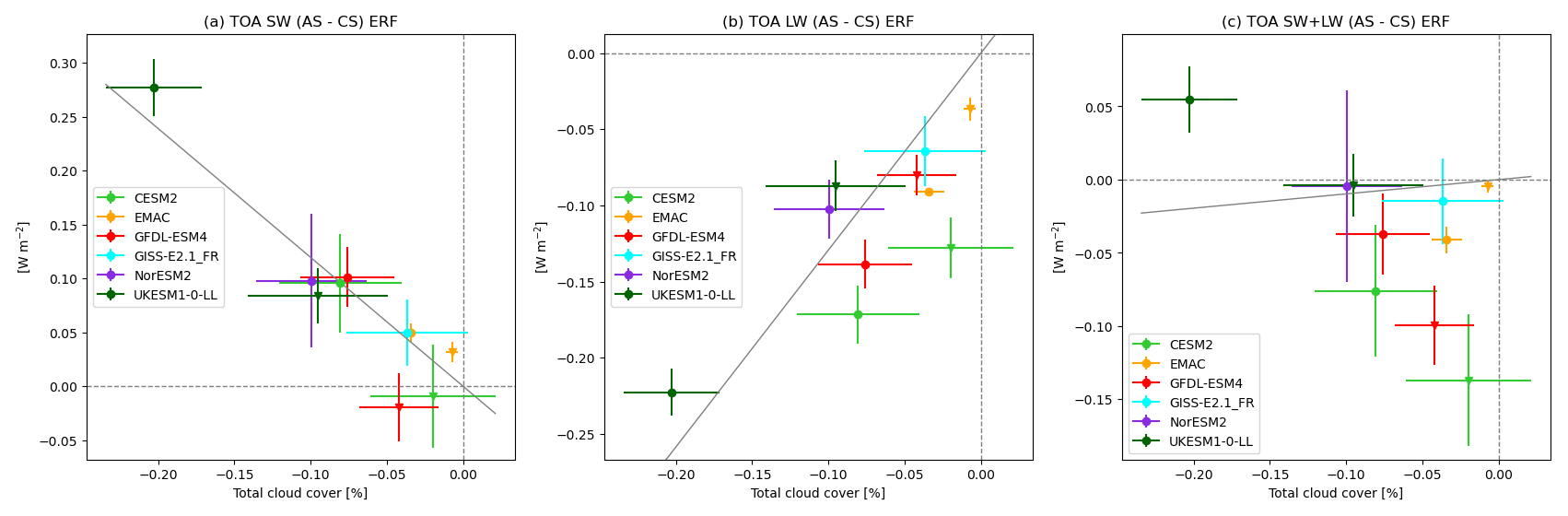
Figure 10 TOA all-sky minus clear-sky short-wave (a), long-wave (b) and short- plus long-wave (c) ERF (in W m⁻²) as a function of the total cloud cover change (in %). Results from the standard experiment pdClim-2050ssp370-radO3 are represented by circles, and results from the sensitivity experiment pdClim-2050ssp370fODS-radO3 are represented by triangles for the four models that did those experiments (CESM2, EMAC, GFDL-ESM4 and UKESM1-0-LL). The error bars indicate the error of the mean, and the line is a best least-squares fit (going through the origin).

Overall the models show a robust decrease in cloud cover in response to increased ozone. This causes a significant increase in SW forcing and a significant decrease in LW forcing, with a small decrease in net forcing that varies across models, contributing to the differences in how rapid adjustments enhance or reduce the ERF compared to IRF.

4.6 Albedo changes

The clear-sky SW ERFs include a component from changes in the surface albedo due to changes in snow and ice cover. Surface albedo was diagnosed as the ratio of the upward and downward clear-sky SW fluxes at the surface. The albedo change can be approximately converted to a clear-sky SW forcing using the formula $\mathrm{\Delta }F=-T_{\mathrm{a}}^{\mathrm{cr}}\times I_{\mathrm{t}}\times \mathrm{\Delta }{\mathit{\alpha }}_{\mathrm{s}}$ (Qu and Hall, 2006), where $T_{\mathrm{a}}^{\mathrm{cr}}$ is the effective atmospheric clear-sky transmissivity (taken to be 0.7), I_t is the incoming SW TOA flux and Δα_s is the change in albedo. Results are shown in Table 6. The change in surface albedo is consistent among the models (apart from EMAC), with a decrease of around 2 × 10⁻⁴. The interannual standard deviation in the surface albedo is large (around 3 × 10⁻⁴), so a few decades of simulation are needed to reduce the standard error of the mean. The EMAC model has the smallest change in albedo. It has a large interannual standard deviation (around 10 × 10⁻⁴), but the nudging ensures this is correlated between control and perturbations so that the interannual standard deviation in the albedo difference is very small (around 0.05 × 10⁻⁴). It appears that nudging the meteorology significantly reduces the albedo response in EMAC.

Table 6 Global mean absolute surface albedo change and associated forcing from pdClim-2050ssp370-radO3 minus pdClim-control. Uncertainties for individual models are errors of the mean. Uncertainties for the multi-model mean are standard deviations across the models. Forcings are calculated using the formula in the text. Only models that provided surface SW fluxes are shown.

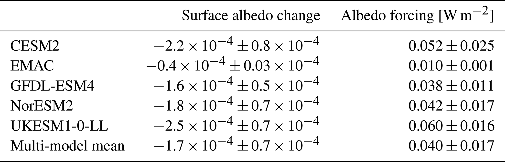
There is a robust decrease in surface albedo, which translates into a positive SW contribution to the ERF.

4.7 Sensitivity of forcing to tropospheric ozone precursors

In this section, the sensitivity of the year-2050 ozone response and the corresponding forcings will be examined, making use of the pdClim-2050ssp370fODS-radO3 (fODS-perturbation) simulation (Table 2), which was carried out by four of the models: CESM2, EMAC, GFDL-ESM4 and UKESM1-0-LL. It should be noted that although halocarbon concentrations are fixed in the fODS-perturbation, nitrous oxide (N₂O) concentrations are not fixed (the possible effects of N₂O changes are discussed later in this section). Our focus here is on pdClim-2050ssp370fODS-radO3 minus pdClim-control tropospheric ozone differences, which will be predominantly driven by increases in tropospheric ozone precursors in 2050 following SSP3-7.0. Figure 11 shows the change in TCO, TrCO and zonal-mean ozone in 2050 relative to the present day from the smaller 4-member ensemble. In 2015, the multi-model global mean TCO of 297.7 ± 8.7 DU is within 1 DU of the full 7-member TOAR-RF ensemble mean shown in Fig. 3 (298.3 ± 8.3 DU), indicating that the 4-member ensemble is representative of the larger 7-member ensemble. Global mean TCO increases by 4.8 ± 0.7 to 302.5 ± 8.3 DU in 2050 in the fODS-perturbation simulation, with the largest increases occurring over the Middle East, India, southeast Asia and the high latitudes in both hemispheres (Fig. 11a). The individual global mean TCO increases range from 3.8 DU in the EMAC model to 5.7 DU in UKESM1-0-LL, with the CESM2 (4.8 DU) and GFDL-ESM4 (4.9 DU) TCO increases close to the 4-member ensemble mean (Table 4). Thus, the TCO increase in the fODS-perturbation explains around 35 % and ODSs around 65 % (i.e. 9.5 ± 2.8 DU) of the TCO increase in pdClim-2050ssp370-radO3 (14.2 ± 3.2 DU; Fig. 11a; Table 4) based on the smaller 4-member ensemble.

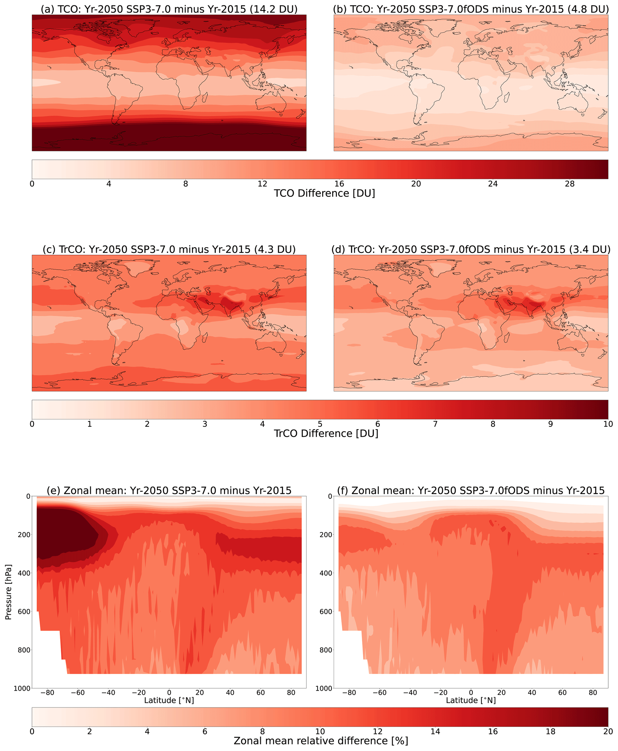
Figure 11 Multi-model mean differences in total column ozone (TCO; panels a and b), tropospheric column ozone (TrCO; panels c and d) and zonal-mean ozone (panels e and f) in 2050 relative to the present day from pdClim-2050ssp370-radO3 (left column) and pdClim-2050ssp370fODS-radO3 (fODS; right column). Panels (a), (c) and (e) are the same as Figs. 3c, 4c and 5c, respectively, but only those models that performed the fODS-perturbation pdClim-2050ssp370fODS-radO3 are shown here as this provides a fairer comparison to panels (b), (d) and (f). Units of TCO and TrCO differences are in Dobson units (DU), while the zonal-mean differences are in %. Models included in the multi-model means are CESM2, EMAC, GFDL-ESM4 and UKESM1-0-LL.

Turning to TrCO, the present-day global mean value of 36.5 ± 1.3 DU is again consistent with the 7-member ensemble (36.2 ± 1.1 DU; Fig. 4). In the fODS-perturbation simulation, year-2050 TrCO increases by 3.4 ± 0.3 to 39.9 ± 1.4 DU. A comparison of TrCO changes in fODS-perturbation (3.4 ± 0.3 DU; Fig. 11d; Table 4) with those from pdClim-2050ssp370-radO3 (4.3 ± 0.3 DU; Fig. 11c; Table 4) indicates that around 75 % of the increase in TrCO is driven by tropospheric ozone precursors and 25 % by decreases in ODSs. This is evident over the Middle East, India and southeast Asia including its outflow regions, where increases in TrCO of 4–8 DU occur. From a zonal-mean perspective, Fig. 11f shows that the largest relative changes in ozone in the fODS-perturbation simulation occur in the southern high-latitude upper troposphere and in the Northern Hemisphere troposphere. This latter region of large relative increase extends from the surface into the upper troposphere (100–300 hPa) in the tropics and extra-tropics, where the radiative efficiency for ozone forcing is highest (Fig. 1).

The global mean all-sky and clear-sky ERF is reduced in the fODS-perturbation compared to the standard perturbation for all models (see Fig. 12). The global multi-model mean all-sky ERF of the four models that performed pdClim-2050ssp370fODS-radO3 decreases from 0.292 ± 0.077 W m⁻² in the standard perturbation pdClim-2050ssp370-radO3 to 0.136 ± 0.035 W m⁻² in pdClim-2050ssp370fODS-radO3; i.e. half of the future ozone ERF comes from increases in tropospheric ozone precursors and half (0.156 ± 0.071 W m⁻²) from decreases in ODSs. In the different models, the all-sky ERF is reduced by around 60 % for CESM2, GFDL-ESM4 and UKESM1-0-LL and by around 23 % for EMAC. In the clear sky, both LW ERF and SW ERF are reduced, with changes in clear-sky ERF being larger in the SW for all models.

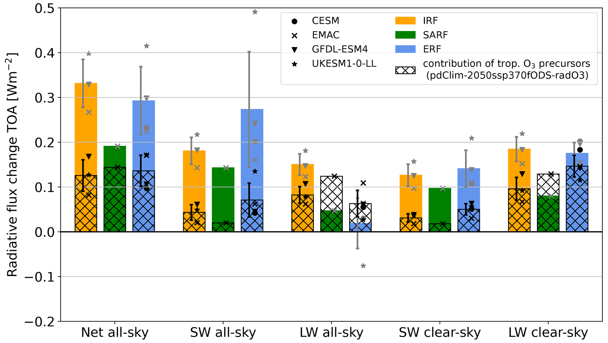
Figure 12 Online-calculated IRF, SARF and ERF for models that performed the fODS-perturbation pdClim-2050ssp370fODS-radO3. The coloured bars represent multi-model mean estimates corresponding to the standard perturbation pdClim-2050ssp370-radO3, whereas the hatched bars represent the contribution of tropospheric ozone precursors, i.e. corresponding to the fODS-perturbation pdClim-2050ssp370fODS-radO3. Only those models that performed the fODS-perturbation pdClim-2050ssp370fODS-radO3 are included in the pdClim-2050ssp370-radO3 estimates to provide a fairer comparison. The multi-model spread is given by the inter-model standard deviation. The markers represent individual model estimates, grey for pdClim-2050ssp370-radO3 and black for pdClim-2050ssp370fODS-radO3.

Global mean all-sky and clear-sky IRF is reduced in the fODS-perturbation compared to the standard perturbation simulation for all models. This is due to reduced IRF both in the SW and in the LW. As can be expected, the increased stratospheric ozone because of the reduction in ODSs in the standard perturbation pdClim-2050ssp370-radO3 leads to additional absorption of SW radiation compared to the fODS-perturbation. In the LW, the trapping of outgoing LW radiation by the additional stratospheric ozone seems to dominate because LW IRF is larger in the standard perturbation compared to the fODS-perturbation. The global multi-model mean all-sky IRF of the three models (CESM2 did not provide IRF data) that performed pdClim-2050ssp370fODS-radO3 decreases from 0.331 ± 0.053 W m⁻² in the standard perturbation pdClim-2050ssp370-radO3 to 0.125 ± 0.035 W m⁻² in pdClim-2050ssp370fODS-radO3.

EMAC is the only model that provides online-calculated SARF for pdClim-2050ssp370fODS-radO3. The corresponding global mean all-sky SARF is estimated at 0.144 ± 0.002 W m⁻² (see Table S7). As discussed in Sect. 4.3, the stratospheric-temperature adjustment is negative (IRF > SARF) in the standard perturbation pdClim-2050ssp370-radO3 for EMAC. This is consistent with the temperature in the stratosphere increasing due to increased stratospheric ozone levels (see Fig. 9h), which leads to a reduced LW forcing for SARF compared to IRF. Figure S9a shows more detail on the stratospheric-temperature profile change for one model (EMAC). Here it can be seen that the increased temperature occurs in the lower and middle stratosphere (roughly from 200 to 20 hPa) and also at around 2 hPa. Temperature changes at higher altitudes have less impact on the net TOA radiative forcing as the density of the atmosphere decreases. In the fODS-perturbation, however, SARF is enhanced by 0.062 W m⁻² compared to IRF due to the decreased stratospheric temperatures as diagnosed by the FDH calculations (see Fig. S9). Note that in Fig. 9h (and Fig. S9a) there is warming in the modelled temperatures in the upper troposphere and lower stratosphere even in the fODS-perturbation that is not captured in the FDH calculations.

From the offline kernel calculation, the total ozone SARF for the ozone precursors in the fODS-perturbation is 0.178 ± 0.018 W m⁻² (Table S8). This is 70 % of the SARF in the standard perturbation (0.254 ± 0.017 W m⁻² for these four models), and thus the ODS contribution is only 30 % (0.076 ± 0.025 W m⁻²). Tropospheric ozone, where the tropopause is defined by the monthly ozone mole fraction in the control simulation, contributes between 71 % and 77 % of the total ozone SARF in the fODS-perturbation for all four models. The tropospheric ozone SARF is presented in Table S9.

We have also analysed the latitudinal distribution of radiative flux changes in the EMAC fODS-perturbation simulation (Fig. S7b). We focus here on EMAC as it is the only model that provides all online diagnostics. Apart from the noisy behaviour of the all-sky ERF, ERF values are generally larger than SARF values, which are larger than IRF values at almost all latitudes. This holds true for both clear-sky and all-sky diagnostics. Comparing the latitudinal distribution of the forcings in the standard perturbation and the fODS-perturbation, the largest changes can be found in the polar regions, in particular over the Antarctic, which highlights the impact of changing ODS abundances on the RF diagnostics.

5 Discussion

The future increases in ozone precursors and decreases in ozone-depleting substances in the SSP3-7.0 scenario lead to an increase in global mean TCO by 12.2 DU between 2015 and 2050 in the multi-model mean, with the 7 individual models included in the ensemble mean showing increases of 4.3 to 19.6 DU. From a multi-model mean perspective, about 4.3 DU (around 39 %) of the global mean TCO changes are attributable to the tropospheric ozone changes, while the rest are due to changes in stratospheric ozone abundances. In a sensitivity simulation in which ODSs in 2050 were kept at year-2015 levels (fODS), the importance of ozone precursor changes was assessed by a subset of models. In the respective multi-model mean, the global mean TCO increases by 4.8 DU, with individual model increases ranging from 3.8 DU in EMAC to 5.7 DU in UKESM1-0-LL (see Sect. 4.7; Table 4).

5.1 Radiative efficiencies

Based on the model-dependent changes in ozone with respect to the standard perturbation simulation, an offline radiative kernel leads to a total SARF of 0.134 to 0.319 W m⁻², with 34 % to 43 % of this forcing coming from changes in ozone above the tropopause (defined as ozone mole fraction values of 150 nmol mol⁻¹; see Sect. 4.4). When scaling the kernel SARF by the total column ozone change (see Fig. 13), the radiative efficiency varies from 0.014 to 0.030 W m⁻² DU⁻¹. For models that show lower increases in stratospheric ozone, their ozone radiative efficiency is towards the higher end of this range, whereas for models showing higher increases in stratospheric ozone, the efficiency is towards the lower end. This is due to the kernel having the highest efficiency in the upper troposphere and lower stratosphere (Fig. 1). When using only the tropospheric column, there is much more agreement on the radiative efficiency with a range of 0.039 to 0.044 W m⁻² DU⁻¹, which is in good agreement with previous findings of a tropospheric ozone radiative efficiency of 0.042 W m⁻² DU⁻¹ in Stevenson et al. (2013). For the fODS-perturbation, the radiative efficiencies for the total column and tropospheric column are in closer agreement, reflecting the smaller effects on stratospheric ozone.

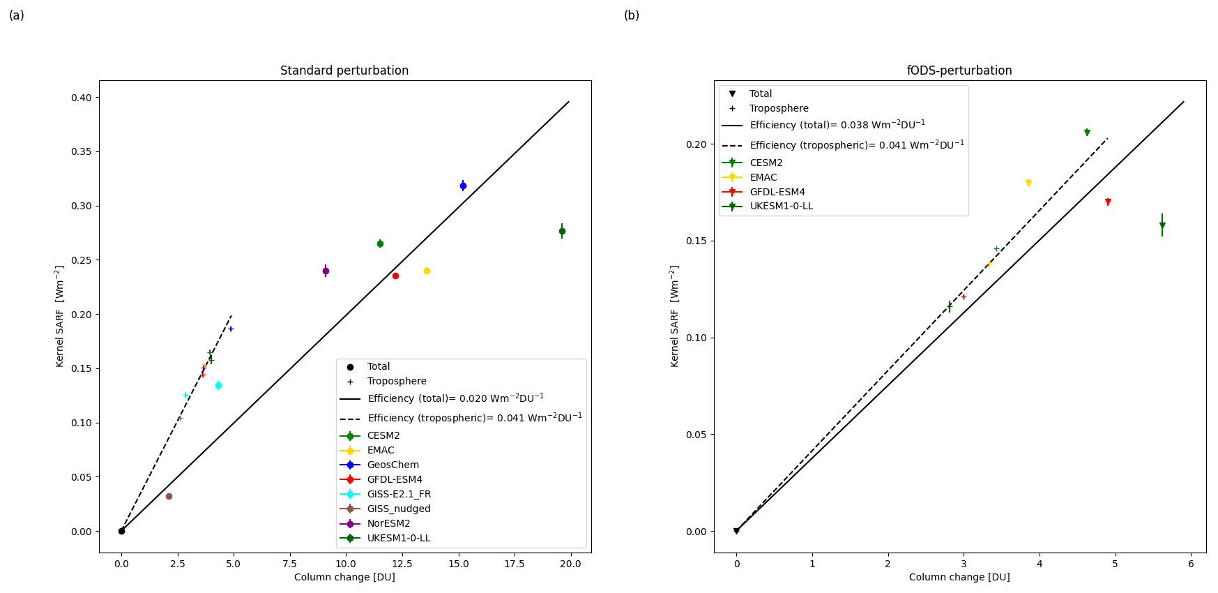
Figure 13 Kernel SARF vs. column ozone change for (a) standard perturbation and (b) fODS-perturbation. Values for tropospheric-only and total column changes are shown.

For the models that separated out the effects of ODS changes, the ERF decreased from 0.292 ± 0.077 W m⁻² in the standard perturbation to 0.136 ± 0.035 W m⁻² with fixed ODSs. The effect of stratospheric ozone recovery (standard minus fODS) was 0.156 ± 0.071 W m⁻², larger than that of ozone precursor increases. This is comparable to the −0.15 W m⁻² contribution of ODSs to the historical ozone forcing as assessed by IPCC AR6 (Szopa et al., 2021); however the corresponding equivalent effective stratospheric chlorine (EESC) decrease over the period 2015 to 2050 is only around 450 ppt (WMO, 2022) compared to a historical increase in EESC of around 1200 ppt up to 2015. Hence using ERF, we find nearly 3 times the sensitivity to ODS changes (−0.34 ± 0.16 W m⁻² ppb(Cl)⁻¹) compared to the IPCC AR6 (−0.12 W m⁻² ppb(Cl)⁻¹). Using the kernel SARF (as used in the AR6 analysis) of 0.076 ± 0.025 W m⁻² gives a radiative efficiency of −0.17 ± 0.06 W m⁻² ppb(Cl)⁻¹, which is consistent with AR6.

Literature estimates of the SARF from 2000 to 2100 (approximate EESC decrease of 1050 ppt) range from 0.05 to 0.16 W m⁻² (Banerjee et al., 2018; Bekki et al., 2013; Iglesias-Suarez et al., 2018). These correspond to a radiative efficiency of −0.05 to −0.15 W m⁻² ppb(Cl)⁻¹.

5.2 Instantaneous radiative forcing

The ozone IRFs are calculated both by the kernel method (Sect. 4.4) and by online double calls to the radiation scheme (Sect. 4.3). There is strong correlation between the two methods in the clear sky (see Fig. 14); however the kernel-calculated IRFs are larger than those calculated online, by around 40 % in the LW. This applies to all models and so seems to be a characteristic of the radiation scheme used to generate the kernel data (Myhre and Stordal, 1997). This large difference between the ESM radiation schemes and the kernel is unexpected and makes comparison between SARF and ERF or IRF more challenging.

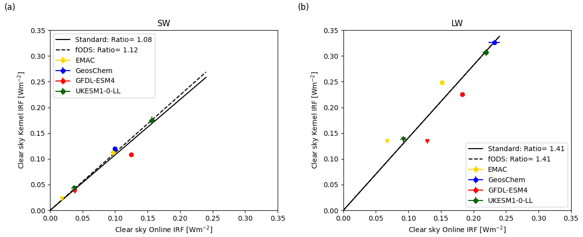
Figure 14 Comparison of the online (double call) and kernel methods for calculating the clear-sky instantaneous radiative forcing (IRF) for (a) SW and (b) LW. Both standard perturbation and fODS-perturbation are plotted.

5.3 Non-cloud adjustments

For changes in tropospheric ozone (Table S6), as a result of stratospheric-temperature adjustments, the SARF calculated by the kernel is between +31 % to +38 % greater than the kernel-calculated instantaneous forcing. Since the adjustments are pre-calculated in the kernels, the variation is due to slight variations in the vertical distribution of the ozone changes in the different models. The adjustments are significantly smaller than in Shine et al. (2022), who found around +80 % adjustment for a pre-industrial to present-day tropospheric ozone change (Checa-Garcia et al., 2018). The adjustments to changes in stratospheric ozone are considerably more variable, from −40 % to −65 %, reflecting the wider variability in the vertical distributions of the ozone changes in the stratosphere. The adjustments in Shine et al. (2022) were larger, −80 % of the IRF for stratospheric ozone changes, but these were dominated by the depletion caused by ODSs, in contrast to this study, where the changes in ozone precursors make substantial contributions in the stratosphere.

5.3.1 Short wave

By excluding cloud effects, the clear-sky ERFs should compare to the kernel SARFs if the tropospheric non-cloud adjustments are small. The modelled clear-sky SW ERF correlates well with the IRF (equal to SARF in SW) kernel calculations (see Fig. 15). The ERF calculation is consistently higher than the IRF (see Table 7). This is also the case using the double-call clear-sky SW IRF for the models that diagnose it. This is expected from the decreases in surface albedo diagnosed in Sect. 4.6. For the fODS experiments, the albedo adjustment explains the difference between the ERF and IRF such that the residual defined as ERF − IRF − adjustment is zero, suggesting that albedo changes explain the difference. In the standard experiments when decreases in ODSs are included, the residual is negative, suggesting that there may be further negative adjustments in the SW as a response to stratospheric ozone recovery. The ozone recovery leads to an increase in stratospheric water vapour (Fig. 9j), but it is not obvious why this would lead to a negative SW forcing adjustment.

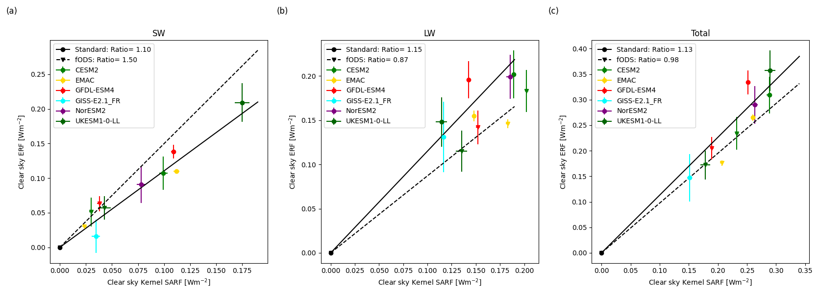
Figure 15 Comparison of clear-sky ERF and SARF from the kernel calculations for (a) SW, (b) LW and (c) total forcing. Both standard perturbation and fODS-perturbation are plotted.

Table 7 Comparison of the difference between ERF and IRF with the albedo adjustment in the clear-sky SW. Two definitions of IRF are used, kernel and double-call. Only a subset of models included double-call diagnostics. The residual is defined as ERF − IRF − albedo adjustment.

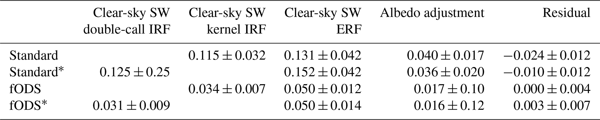
^* Only models that included the double-call diagnostic of IRF.

In this study we define the ERF using fixed SSTs. If land temperatures were also fixed, it is likely that the albedo adjustment would be substantially reduced. If an ERF defined using fixed SSTs and land temperatures were required, as in IPCC AR6 (Forster et al., 2021), then it would be necessary to subtract the albedo adjustment from the diagnosed fSST ERFs. This would be analogous to subtracting the land surface temperature adjustment as in Tang et al. (2019).

5.3.2 Long wave

We do not have a clear-sky LW SARF kernel, so for comparison with the clear-sky ERF, we add the all-sky kernel stratospheric-temperature adjustment to the clear-sky kernel IRF, assuming the stratospheric-temperature adjustment is unaffected by cloud (which is the case with the online SARF calculations by EMAC). In the LW there is a positive correlation between clear-sky ERF and SARF (Fig. 15b). For fODS, the ERF results are lower than the SARF kernel, which is in line with the kernel IRF being larger than the online calculations in the models (Sect. 5.2). This makes it difficult to draw any conclusions on the relative contributions of the negative adjustments due to the increases in tropospheric temperature seen in Fig. 9h versus the positive adjustments due to increases in water vapour in Fig. 9j. For the standard perturbation, the larger LW clear-sky ERF than kernel SARF implies positive adjustments that are likely to be due to the large increases in stratospheric water vapour in Fig. 9e and j when ODS changes are included. For the EMAC model, the stratospheric-temperature change diagnosed online by FDH is larger than that generated in the ESM (see Fig. S9) in the lower and middle stratosphere, particularly in the Southern Hemisphere, suggesting that the stratospheric-temperature adjustment assuming FDH might be too strongly negative in terms of forcing. Comparison of the latitudinal distribution of ERF, SARF and IRF in the EMAC model (Fig. S7) shows that, when excluding ODSs, the ERF matches the SARF, but when changes in ODSs are included, the IRF is a better representation of the ERF than the SARF.

This difference between the ERF and the SARF is even greater when subtracting the fODS from the standard perturbation (i.e. the effect of ODSs). The mean LW clear-sky ERF (standard minus fODS) of the four models in Fig. 15b is 0.028 ± 0.017 W m⁻², but the SARF is −0.020 ± 0.010 W m⁻².

5.3.3 Summary of clear-sky comparison

Both experiments show a decrease in surface albedo, with a consequently larger SW clear-sky ERF than SARF. This has a proportionally greater effect for fODS-perturbation. In the LW clear sky the ERF is larger than the kernel SARF for the standard perturbation. For the effect of ODSs (standard minus fODS), the LW clear-sky ERF even has a different sign. This sign change between LW clear-sky ERF and SARF is also the case for the EMAC model, which diagnoses both online. Since the kernel LW IRF was found to be 40 % greater than that of the models (Sect. 5.2), the true increase in ERF compared to the SARF could be even larger.

5.4 Cloud adjustments

There are large adjustment terms that are found to be due to changes in the cloud fraction (Sect. 4.6, Table 5). Note that the difference between all-sky and clear-sky ERF is not solely due to cloud adjustments but includes a contribution from cloud masking of the ozone forcing. The models agree on a reduction in the upper-troposphere cloud fraction and (apart from UKESM1-0-LL) an increase in the mid-troposphere cloud fraction. In the lower troposphere, there is less agreement, with some models showing a decrease in cloud fraction around 800 hPa and an increase just above the surface. This is generally in agreement with a study by MacIntosh et al. (2016), who found stratospheric ozone depletion increased high cloud and upper-troposphere ozone increases decreased high- and medium-level cloud but increased low cloud. Grise et al. (2013) found that Antarctic ozone depletion also causes changes in the latitudinal distribution of clouds. There are strong correlations between the changes in the cloud fraction and the cloud adjustments in the SW and a weaker correlation in the LW. Reduced cloud cover gives a positive SW adjustment due to decreased planetary albedo and a negative LW adjustment as reductions in high cloud increase the overall emitting temperature of the atmosphere. These two adjustments largely cancel each other out, with the larger LW adjustment leading to an overall negative cloud adjustment. The exceptions are UKESM1-0-LL (standard perturbation), which has a strong positive SW adjustment, and NorESM2 (standard perturbation), which has a weaker LW adjustment. The cloud changes and associated SW and LW adjustment in the fODS-perturbation (Table S10) are smaller, highlighting the stronger effect of stratospheric ozone changes on clouds. Because the overall adjustment is the compensation of two opposing terms, there is no correlation with the change in cloud fraction. There is a suggestion that the cloud adjustment is negative for the ozone precursor changes and positive for the ODS changes, but the uncertainties are large. Although uncertain, the cloud adjustment (−0.1 to +0.05 W m⁻²) is a significant fraction of the total ERF (0.27 ± 0.08 W m⁻²).

6 Conclusions

We have shown that projected increases in tropospheric ozone precursors and decreases in ODSs in the SSP3-7.0 scenario lead to increases in ozone in the troposphere and stratosphere. By restricting the impact of composition changes on the evolution of the physical model, we can isolate the changes solely due to changes in ozone. This contributes an ERF of 0.268 ± 0.084 W m⁻² from 2015 to 2050. This is larger than the forcing of 0.19 W m⁻² assessed by IPCC AR6 for this period and scenario (Dentener et al., 2021) and would make ozone the second largest contributor to warming over this period due to the combination of the forcing from stratospheric ozone recovery and the increases in ozone precursor emissions in this scenario.

A subset of models calculated the ERF excluding ODS changes. These show that ozone precursor increases and ODS decreases contribute approximately equally to the total ERF change. The future contribution of ODSs to ozone ERF is comparable (though of opposite sign) to the contribution of ODSs to the historical ozone forcing as assessed by IPCC AR6. This would make the indirect radiative efficiency of ODSs (in forcing per change in equivalent effective stratospheric chlorine) almost 3 times that assessed in the IPCC and WMO (2022). The increase in ozone forcing expected from commitments to reduce ODSs could therefore offset most of the climate benefits from reducing their direct greenhouse effect.

ERF and SARF diagnosed from the offline kernel agree within the uncertainty range for the combined effect of ozone precursor and ODS changes. However the difference between ERF and SARF becomes more apparent when looking at the ozone precursors and ODSs separately. The SARF with fixed ODSs is higher than the ERF, which could be explained by systematically higher kernel results (since this is not the case for the online-calculated SARF in the EMAC model). The SARF due to ODS changes is significantly lower than the ERF, which suggests that the fixed dynamical heating approach used in the SARF overestimates the temperature increase in the stratosphere from stratospheric ozone recovery and that there is an additional contribution to the ERF from increasing stratospheric water vapour. The radiative adjustment due to reduced surface albedo is significant and positive.

Ozone increases from both ozone precursors and decreasing ODSs consistently reduce cloud cover in the upper troposphere, with most models finding increased cloud cover in the mid-troposphere. This leads to significant radiative adjustments that are negative in the LW and positive in the SW. The net effects of clouds largely cancel each other out, giving a net adjustment that is not significantly different from zero (slightly negative from ozone precursor increases, slightly positive from ODS decreases).

This study shows that care is needed when interpreting or comparing radiative forcing calculations for ozone. While the radiative forcing calculated as ERF or SARF is similar for the combined effects of tropospheric ozone precursors and ODSs, this is not true for the ozone precursors and ODSs separately. Here, we find that the kernel-calculated SARF is a factor-of-2 lower than the ERF for the ozone radiative forcing from ODS changes, highlighting a need to compare offline radiative transfer modelling against a full Earth system model.