Ozone (O₃) observations in Saxony, Germany, for 1997–2020: trends, modelling and implications for O₃ control

Given its importance for human health, vegetation and climate, trends in ground-level ozone (O₃) concentrations in eastern Germany were systematically analysed using the long-term O₃ data from 16 measurement stations. The findings indicate that despite reductions in oxides of nitrogen (NO_x= NO + NO₂) concentrations across all sites, O₃ pollution in Saxony has in fact worsened over the past decade, especially in densely populated urban areas. The strongest O₃ trend is observed at a traffic-dominated station, with an annual ozone increase of 1.2 µg m⁻³ yr⁻¹ (or 3.5 % yr⁻¹), while urban and rural background stations show more moderate rises of, on average, 0.5 µg m⁻³ yr⁻¹ (or 1.1 % yr⁻¹) over the last decade.

To diagnose O₃ formation and the controlling effects of NO_x and volatile organic compounds (VOCs) over the past decades in this region, for the first time, detailed photochemical box modelling was performed by means of the complex MCM (Master Chemical Mechanism). Analysis of isopleth diagrams for two seasons indicates that O₃ formation was predominantly VOC-limited at traffic and urban sites from 2000 to 2019. The observed rise in O₃ levels suggests that current efforts to reduce total non-methane volatile organic compound (TNMVOC, including NMVOCs and oxygenated VOCs) emissions and NO_x from various sources unfortunately remain insufficient. Based on anthropogenic and biogenic emission data, we recommend that continued NO_x abatement and further additional VOC controls, with a focus on solvent use, be implemented in densely populated areas to mitigate O₃ pollution in the coming years.

1 Introduction

Tropospheric ground-level ozone, acting simultaneously as a key oxidant and a greenhouse gas, has adverse effects on human health, vegetation such as forests and agricultural crops, and the Earth's climate as a short-lived climate forcer or SLCF (Lefohn et al., 2018; Agathokleous et al., 2020). Apart from typical climate conditions causing the intrusion of stratospheric O₃ from high elevations (Lin et al., 2015; Wang et al., 2020) and long-range atmospheric transport from polluted places (Derwent and Parrish, 2022; Mathur et al., 2022), primarily emitted oxides of nitrogen (NO_x= NO + NO₂), carbon monoxide (CO) and volatile organic compounds (VOCs) are the key precursors, which form O₃ in a complex photochemical reaction system depending on the prevailing chemical regime (Crutzen, 1973; Seinfeld and Pandis, 1998, 2016).

The highly nonlinear O₃ chemical formation has always been the biggest challenge in controlling ozone pollution. It is widely acknowledged that O₃ formation can be limited by VOCs or NO_x or coupling-limited by both VOCs and NO_x (Seinfeld and Pandis, 2016). In the “NO_x-limited” regime, reductions in NO_x emissions lead to the most effective O₃ reduction. Conversely, in the “VOC-limited” regime, reductions in VOC emissions show the greatest reduction of O₃ pollution, while reductions in NO_x actually increase O₃ formation rates. In densely populated European metropolitan areas (e.g. Milan, Athens, Berlin and Paris) with high NO_x emissions, O₃ production tends to be VOC-limited or in a transitional regime, whereas in rural and other background areas (such as mountain and ocean sites) it is typically under NO_x-limited regimes (Hammer et al., 2002; Gabusi and Volta, 2005; Bossioli et al., 2007; Deguillaume et al., 2008; Beekmann and Vautard, 2010; Melkonyan and Kuttler, 2012; Mar et al., 2016; Feldner et al., 2022).

Europe launched the Gothenburg Protocol of 1999 to limit emissions from fossil fuel combustion associated with motor vehicles and power plants, resulting in emission reductions, compared to 1990, of 63 % (NO_x) and 59 % (NMVOCs) in 2021 (EEA, 2023). It should be noted that the decline in VOCs has plateaued since 2010, unlike the continued reduction in NO_x.

Continuously reduced emissions led to successful mitigation of peak O₃ pollution, as reflected in decreasing or stagnant peak O₃ levels across most ground-based observations (Paoletti et al., 2014; Derwent et al., 2018; Fleming et al., 2018; Yan et al., 2018; Boleti et al., 2019; Ronan et al., 2020), except at remote, high-altitude sites due to the dominant influence of hemispheric background ozone (Gilge et al., 2010; Boleti et al., 2019).

Despite decreasing peak levels, O₃ mean concentrations show opposite and often increasing trends over the last nearly 30 years across most traffic, suburban and urban sites, as well as some rural sites (Salthammer et al., 2018; Yan et al., 2018; Diaz et al., 2020). In the recent 10–15 years, stronger O₃ increases for certain urban areas compared to rural sites have been identified (Salthammer et al., 2018; Sicard et al., 2020; Sicard, 2021). At remote or alpine background sites, mean O₃ levels have remained stagnant or have shown only slight increases since 2000 (Cristofanelli and Bonasoni, 2009; Parrish et al., 2012; Cooper et al., 2014, 2020).

Following the clear main trend, many studies have been directed at exploring the causes of rising O₃ levels in different geographic areas, which were attributed to different possible reasons, including reduction of anthropogenic emissions of NO_x and therefore a weakening of the NO titration effect (Sicard et al., 2020; Sicard, 2021), higher biogenic VOC emissions (Curci et al., 2009; Bonn et al., 2018; von Schneidemesser et al., 2018), emissions from the land transport sector (involving road traffic, inland navigation and trains) (Mertens et al., 2020), specific synoptic meteorological condition in favour of horizontal downwind transport and vertical transport (Huszar et al., 2016; Kalabokas et al., 2017), effects from increasing temperature (Melkonyan and Wagner, 2013) or even extreme weather such as heat waves (Yan et al., 2018), higher CH₄ emissions from increased frequency of biomass burning (Derwent et al., 2007; Cape, 2008), the net impacts of climate change leading to a so-called climate penalty (Colette et al., 2015a; Lin et al., 2020; Otero et al., 2021), or increasing background O₃ levels through long-range transport from polluted areas and increased emissions in Asia (Jenkin, 2008; Derwent et al., 2015; Gaudel et al., 2018; Mertens et al., 2020). Although extensive efforts have been made to reveal possible reasons for increasing O₃ trends, the complex relations between O₃ formation and its drivers in different geographic areas are still not fully understood.

For Germany, a number of studies on long-term (>10 years) changes in ground-level O₃ across different geographic areas have been done over past decades (Melkonyan and Kuttler, 2012; Eghdami et al., 2020; Gebhardt et al., 2021). Most studies focus on discussing O₃ trends in Germany over a specific period, with few comparing mean trends over the past 10, 20 or even 30 years and explaining how ozone has changed in response to variations in anthropogenic emissions. Generally, and to a certain extent surprisingly, available annual mean ground-level O₃ observations have largely remained stable since 2000 (Cooper et al., 2014; Salthammer et al., 2018; Eghdami et al., 2020) despite the continuous reduction of O₃ precursors. For the trends of daily O₃ in urban Germany, Sicard et al. (2020) observed a decrease in the period spanning 2005–2010 and an increase in 2010–2018 and pointed out that the insufficient or inappropriate reduction of anthropogenic emissions had shifted German cities from NO_x-limited to VOC-limited chemistry depending on the ratio of VOCs to NO_x. Thus, a rising trend for O₃ over the last decade might have resulted from the lack of significant further reductions in VOC emissions. However, this finding and attribution are in contrast to other studies which determined the O₃ precursor sensitivity with different methods (Ehlers et al., 2016; Otero et al., 2021). For example, in contrast to the conclusion from Sicard et al. (2020), Otero et al. (2021) defined a slope of ozone–temperature relationship based on generalised additive models (GAMs) to analyse the O₃ precursor sensitivity using summertime observations of O₃ and NO_x from two periods (1999–2008 and 2009–2018) and concluded that a great number of the German stations including urban and rural areas showed at all summer temperatures a tendency to move to a NO_x-limited chemistry with time. Ehlers et al. (2016) modelled local ozone production rates as a function of OH reactivity of VOCs and NO₂ to reveal that under typical summertime conditions, German city sites were located in the VOC-limited regime from 1994–2014, and they pointed out that the modelled strong reduction of local ozone production was derived mainly from a much slower reduction of traffic NO_x compared to VOC emissions.

Regarding ozone exposure as O₃ impacts on human health and vegetation, Sicard et al. (2021) reported the EU-28 urban population was still exposed to O₃ levels widely exceeding the WHO limit values for the protection of human health from 2000 to 2017, despite the significant reductions of emissions. The growing risk of potential O₃ damage due to increasing stomatal ozone can affect both forest and food plants. Regarding forests, data from 2000–2014 have been investigated by Proietti et al. (2021), and so far in Europe, and even more seriously in central Europe, the target value (5000 ppb) for the protection of vegetation has been exceeded as the AOT40 value, an accumulative dose over a threshold value of 40 ppb.

Overall, chronic O₃ levels in Germany continue to be a challenge in terms of air quality and impacts on vegetation and human health. Therefore, the present study focuses on the observed trends of O₃ concentrations at 16 measurement stations in the federal state of Saxony in eastern Germany. It contrasts the mean trends of different station types, different concentration levels and different seasons in three time periods and then applies air parcel photochemical modelling to comprehensively evaluate the efficiency of precursor controls on the observed Saxony O₃ trend over the past decades. All in all, the present comprehensive analysis aims to aid O₃ pollution control policy in the coming years in Germany.

2 Methods and data availability

2.1 O₃ and other pollutant observations in Saxony

Hourly values of ground-level O₃ concentration between 1997 and 2020 were provided by the air quality monitoring network of the Saxon State Office for the Environment, Agriculture and Geology (LfULG, 2025). Figure 1 shows the location of the measuring stations, colour-coded according to traffic stations, stations in the urban or rural background, and stations on the ridge of the Ore Mountains, situated at altitudes between 785 and 1214 m a.s.l. Stations with less than 10 years of ozone data were excluded and are not shown in Fig. 1. Data analysis was done for 16 stations, including 1 traffic station, 7 urban background stations, 4 rural background stations and 4 stations on the Ore Mountains ridge. The temporal data coverage at the station varies, as some of them were opened after 1997 only. The exact periods of O₃ measurements for each station in the air quality monitoring network are shown in Table S1 in the Supplement. Data availability within the measurement periods was very good at all stations, with missing fractions <5 %.

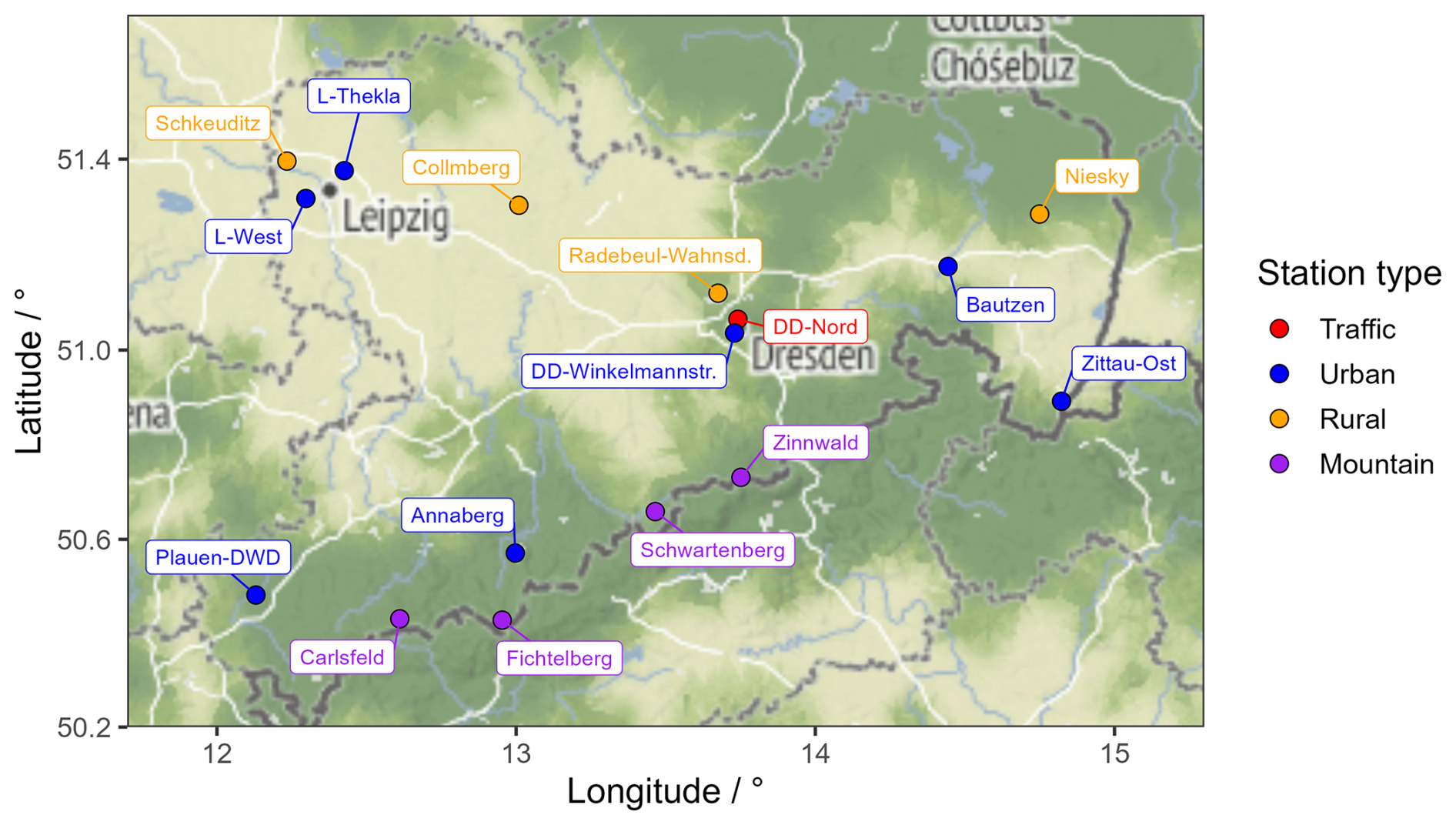
Figure 1 Map of ozone measuring stations in the Saxony air quality monitoring network that provided data for the present study. Map produced using the ggmap package (v4.0.0; Kahle and Wickham, 2013) in R (R core team, 2020) with contributions from © Stadia Maps (2024), © Stamen Design (2022), © OpenMapTiles (2024) and © OpenStreetMap contributors (2024). Distributed under the Open Data Commons Open Database License (ODbL) v1.0.

In addition to the hourly O₃ values, the concentrations of other air pollutants, NO, NO₂ and NO_x, were provided as well. The data available at the respective station are summarised in Table S2, which include nitrogen oxides (NO, NO₂ and NO_x) and the meteorological parameters temperature, global radiation, relative humidity, wind direction, wind speed and air pressure.

2.2 Trend analysis

To determine a robust linear trend of O₃ concentrations, the nonparametric Theil–Sen estimator according to Sen (1968) was used, which requires no prior assumptions about the statistical distribution of the data and is resistant to outliers. For the calculation, the Theil–Sen function of the package openair (Carslaw and Ropkins, 2012) in R (R Core Team, 2020) was used, which calculates a straight line and its slope between all points in the data. The median of the slopes of all straight lines then represents the linear trend of the data. The trends were calculated based on monthly averages per station. To ignore the typical annual variation in O₃ concentration, a seasonal trend decomposition using a locally weighted scatterplot smoothing (LOESS) function is performed within the openair function before the trend calculation when monthly means are used. Furthermore, the openair Theil–Sen function derives p values (probability) and uncertainties by bootstrap simulations. The statistical significance of the calculated trend is represented with symbols as follows: $p<\mathrm{0.001}{=}^{***}$, $p<\mathrm{0.01}{=}^{**}$, $p<\mathrm{0.05}{=}^{*}$ and $p<\mathrm{0.1}=+$. In this paper, all trends with a significance level (probability of error) of 5 %, i.e. from p<0.05, which corresponds to at least one asterisk, are considered statistically significant.

2.3 Photochemical model simulations

To understand the role of photochemistry for O₃ concentration evolution in Saxony, photochemical simulations were performed with the air parcel box model SPACCIM (SPectral Aerosol Cloud Chemistry Interaction Model). SPACCIM combines a size-resolved multiphase chemistry model with a microphysical model, enabling both to function independently while accounting for their interdependencies. Detailed descriptions of the SPACCIM framework can be found in Wolke et al. (2005). In the present study, only the detailed near-explicit gas-phase chemistry mechanism, MCM v3.3.1, is used, which comprises 17 224 reactions (http://mcm.york.ac.uk/MCM/, last access: 1 August 2025) (Saunders et al., 2003).

Simulations with two sets of meteorological scenarios were performed, i.e. (i) summer (June, July and August) and (ii) winter (December, January and February) conditions. All scenarios were driven by anthropogenic and biogenic emission values, meteorological conditions, initial concentrations, and deposition rates.

The summer and winter emission data (Table S3) were based on anthropogenic and biogenic emission inventories in 2019 from the German Environment Agency (UBA) (https://www.umweltbundesamt.de/, last access: 1 August 2025), the Joint Research Centre (JRC) (https://joint-research-centre.ec.europa.eu/, last access: 1 August 2025) and Thürkow et al. (2024), and derived for the whole Saxony area (50.9° N latitude and 14.3° E longitude) (see Fig. S1 in the Supplement showing NO_x emissions of the main roads and urban centres). Besides emission values, other initial parameters had to be adjusted to their typical daytime and nighttime levels under rural conditions (see Table S4 for details). For meteorological parameters and trace gas concentrations (except SO₂, HONO and PAN), data were derived from measurements in Sect. 2.1. The air temperature was set to 15 °C in summer and 4 °C in winter. The pressure was kept constant at 1000 hPa for both seasons, while the relative humidity was maintained at 70 %. The ratio of solar radiation, defined as the mean value between 10:00 and 13:00 divided by the maximum clear-sky radiation value during the same period, was calculated as 0.7 in summer and 0.4 in winter.

The initial SO₂ concentrations in summer and winter were obtained from UBA (https://www.umweltbundesamt.de/daten, last access: 1 August 2025). CO and CH₄ were set to 153.4 and 1700 ppb, respectively, according to the measured data from Zellweger et al. (2009) and Herrmann et al. (2000). Nitrous acid (HONO) and peroxy acetyl nitrate (PAN) concentrations that were not measured at any site were set to the same mixing ratio (0.5 ppb) based on the measurement mean values in Stieger et al. (2018) and Pandey Deolal et al. (2014), respectively. An important aspect of the simulations was to constrain the dry deposition rates of gases, which depends strongly on vegetation cover (Clifton et al., 2020). Considering the different seasonal vegetation covers, different dry deposition velocities (in cm s⁻¹) were considered for NO₂, N₂O₅ and O₃ during summer (NO₂ of 0.3 cm s⁻¹; Rondón et al., 1993), N₂O₅ of 100 cm s⁻¹ (considering dry deposition and aerosol uptake; Zhu et al., 2020), and O₃ of 0.8 cm s⁻¹ (Clifton et al., 2020), as well as winter (NO₂ of 3 cm s⁻¹, N₂O₅ of 2 cm s⁻¹ and O₃ of 0.08 cm s⁻¹) conditions. Dry deposition velocities of other various inorganic gases, such as peroxy acetyl nitrates (PANs), peroxides, carbonyls and acids, were kept the same in both seasonal simulations and are based on the previous urban or rural scenario setup of CAPRAM initialisations (Wu et al., 2012; Hoffmann et al., 2019; Zhu et al., 2020). It should be noted that different boundary layer heights (BLHs) were assumed for the calculation of the respective emission value. The BLHs in the simulations were set to 500 m at night and 2000 m during daytime in summer and to 250 m at night and 1000 m during daytime in winter based on previously available measurements in Germany (Wiegner et al., 2006; Brümmer et al., 2012; Kotthaus et al., 2023). The detailed initial input data (including meteorological conditions, deposition rates, BLHs, chemical initial gas-phase concentrations, e.g. NO₂, O₃, SO₂, CO) for the two seasonal cases are summarised in Table S4.

To initialise the model as comprehensively as possible, a pre-run for each seasonal scenario was performed. Each pre-run simulation was run for 10 d to have an almost steady-state system with stabilised intermediate products, e.g. radicals (OH, HO₂) and oxygenated VOCs (OVOCs) and other VOC (e.g. alkanes and chlorinated VOCs) concentrations that were not measured at the sites of this study. The initial time of both runs was set to 00:00 Central European Time (CET) on 14 July 2019 (summer case) and 14 January 2019 (winter case). The output concentrations from the last day of the pre-run simulations were used as the initial and boundary chemical data for the final 24 h modelling. Dominant initial concentrations are given in Table S5. Moreover, the results of the final 24 h summer and winter scenario simulations (defined as the base case simulations) were used to compare with the measured average diurnal patterns of O₃, NO and NO_x in both seasons at rural background sites to assess the performance of the model simulations. The good agreement of the base case simulations with measurements (see Sect. 3.3 for details) indicated that the model configuration was able to accurately describe the sensitivities of O₃ photochemistry to its different precursors and impact factors.

To gain a deeper understanding of the O₃ trend in the studied area over the past two decades, further photochemical sensitivity simulations were used to derive seasonal isopleth plots of the O₃ formation rates under typical summer and winter conditions in Saxony. These isopleths should help derive a more effective O₃ control strategy by examining O₃ photochemical production against varying levels of NO_x and total non-methane volatile organic compound (TNMVOC, including NMVOCs and OVOCs) emissions across station types. The sensitivity simulations were done by scaling the base case emissions of TNMVOC and NO_x 20 times in each of up to three batch runs for each season; i.e. each combination is considered (Table S6). Three batches were performed to achieve a sensible range of resulting TNMVOC and NO_x concentrations in the total of 800 and 1200 model runs for summer and winter, respectively. The averaged instantaneous rate of net ozone production (NetPO₃) during noontime of 12:00–13:00 CET for each simulated scenario in both summer and winter conditions was determined for each run. The meteorological conditions and settings for all sensitivity simulations in both summer and winter were identical to those of the base case simulations for each respective season. Upon completion of the simulations, the isopleth plots were generated by interpolating the resulting formation rates to a regular grid in the TNMVOC vs. NO_x space and then fitting the O₃ isopleths to it. The plots illustrate the NetPO₃ in relation to the combined ambient concentrations of NO_x and TNMVOCs. Subsequently, leveraging data on NO_x and TNMVOC emissions spanning the past two decades (2000, 2005, 2010, 2015 and 2019), we were able to track changes in O₃ formation over this period by examining variations in seasonal isopleths among different station types. This allowed for a comprehensive assessment of the effectiveness of precursor controls in Saxony over time.

3 Results

Knowledge of O₃ concentrations and trends is important for assessing the effectiveness of existing air pollution control measures and for providing clues for formulating more appropriate control measures in the future. Based on this, first of all, the longer-term changes in the concentration of ground-level O₃ at the stations of the Saxony air quality measurement network are examined and presented. Secondly, the mean trends of ozone concentrations in view of different station types, different concentration levels and different seasons are contrasted in three time periods: (i) during the entire period of available measurement data, i.e. from 1997 or later, (ii) during the 15 years from 2006 to 2020, and (iii) during the more recent 10 years from 2011 to 2020. Finally, and third, photochemical modelling was performed and shifts in O₃ formation regimes for different station types were then attributed to changing emissions over the past 20 years.

3.1 Ozone concentrations and trends

3.1.1 O₃ concentrations

Figure 2 shows the distribution of O₃ concentrations at the individual monitoring stations. The highest concentrations were observed on the Ore Mountains ridge. The mean range of O₃ concentrations on the mountain ridge was from 69 µg m⁻³ at Schwartenberg (785 m a.s.l.) to 78 µg m⁻³ at Fichtelberg (1214 m a.s.l.). The highest single hourly value to date was 282 µg m⁻³ at Schwartenberg. The lowest mean concentrations were observed at the one traffic station in the dataset (Dresden-Nord, hereinafter referred to as DD-Nord): 32 µg m⁻³. Urban background stations showed slightly higher means, depending on the station, of between approximately 40 and 55 µg m⁻³. In the rural background, one station closer to the city, Schkeuditz, showed a somewhat lower mean concentration level, while the other three stations, Collmberg, Niesky and Radebeul-Wahnsdorf, showed slightly higher values of approximately 55–60 µg m⁻³.

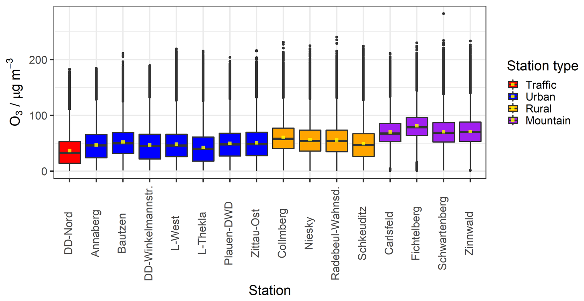
Figure 2 Box plots of O₃ concentrations at individual monitoring stations, coloured according to their station type. The middle yellow point and the black horizontal line indicate the mean and median, respectively. The ends of the box indicate the lower and upper quartiles and the antennas the 1.5-fold interquartile range (IQR), and individual points are extreme values outside the IQR. Data are shown per station from 1997 or later onward to 2020. The detailed station data are summarised in Table S1.

In Fig. 2, the trend of O₃ mean concentrations, which tends to increase from traffic stations towards the Ore Mountains ridge, shows the regional character of O₃. On the one hand, O₃ was formed in the regional background from anthropogenic and biogenic precursor substances; on the other hand, it is degraded by reaction with NO close to NO_x sources such as traffic sites. At the Ore Mountains ridge (>780 m), increased mixing concentration from the free troposphere can also play a role. In general, tropospheric O₃ generally shows increasing concentrations with increasing altitude (Davies and Schuepbach, 1994; Cristofanelli and Bonasoni, 2009; Petetin et al., 2016; Li et al., 2018). This is not only due to stronger mixing from higher layers but also due to lower sink strengths, e.g. the reaction with NO or lower deposition fluxes.

3.1.2 O₃ trends

Generally, the trends in O₃ concentrations do not necessarily change monotonically over different long periods of time, and also, at many of the studied sites, shorter periods of increasing, stagnant or decreasing values were seen (Fig. S2). The magnitudes of linear trend estimates therefore depend on the exact time period considered. In addition, the comparison of mean linear trends across several stations is often complicated by differences in data coverage at the respective stations. Therefore, several Theil–Sen trend calculations were carried out for all stations in three different time periods: (i) during the entire period of available measurement data, i.e. from 1997 or later, (ii) during the 15 years from 2006 to 2020 (with the exception of the DD-Winkelmannstr. station, where O₃ measurements only started from 2008), and (iii) during the more recent 10 years from 2011 to 2020. The reasons for selecting these periods were that, on the one hand, O₃ measurements at almost all stations were available from 1997 at the earliest, and, on the other hand, the trends of more recent years may reflect future trends better than longer-term trends including earlier decades. Detailed information on trends of the individual stations is shown in Table S7 for each time period in absolute and relative values, and all trends are summarised in Fig. 3.

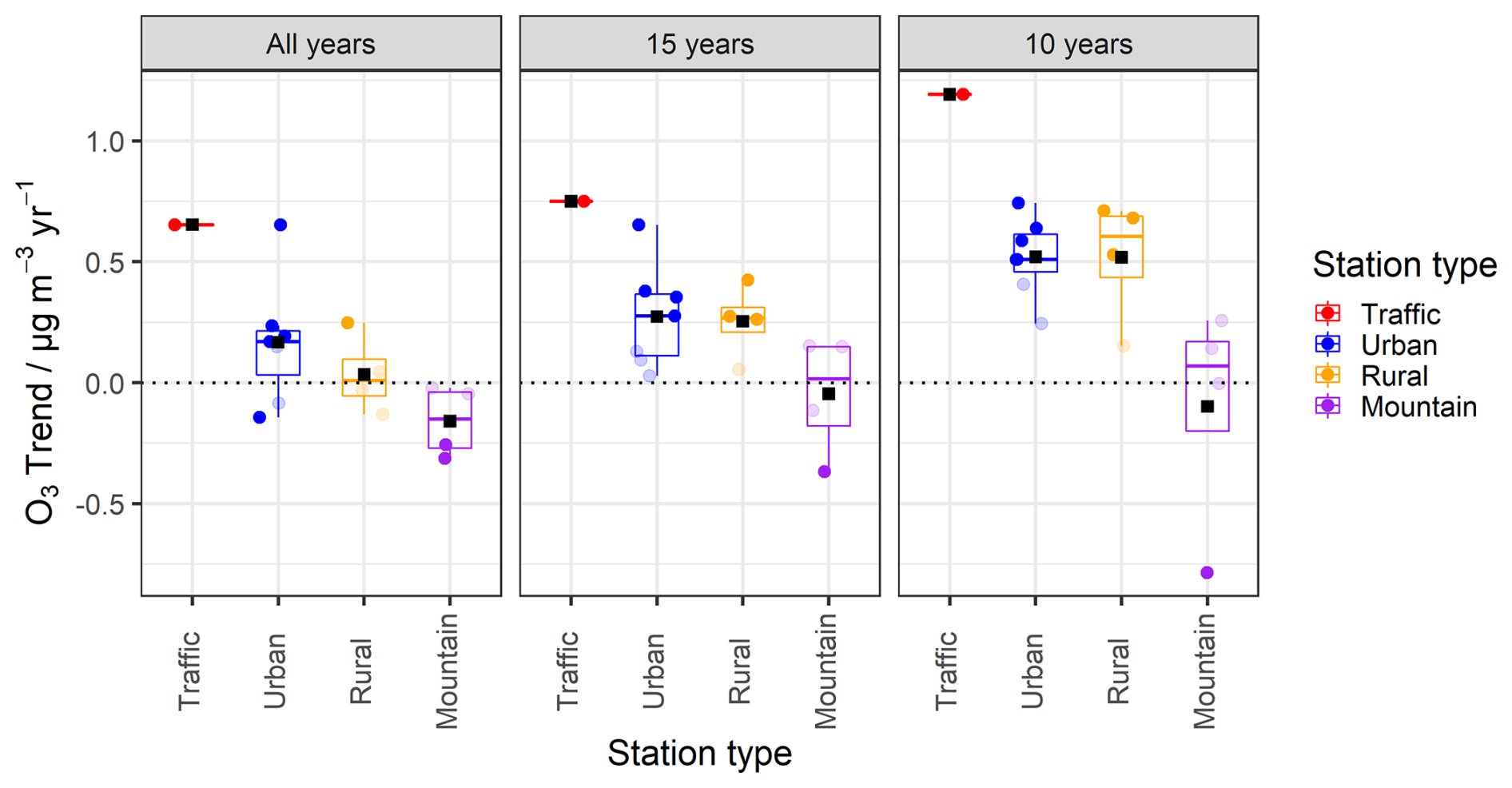
Figure 3 Box plots of observed O₃ trends over three time periods until 2020 (given in columns 1–3) at the four station types. Transparent dots indicate statistically non-significant values. Black squares indicate means across all station values.

Traffic-dominated sites

In Fig. 3 and Table S7, the increasing trend at the traffic site DD-Nord in the recent 10 years is roughly 1.20 µg m⁻³ yr⁻¹ or 3.50 % yr⁻¹ and has nearly doubled compared to 0.65 µg m⁻³ yr⁻¹ or 2.30 % yr⁻¹ over the whole period since 1997. Similarly, most urban sites have also shown a more rapid O₃ increase in the last decade, up to 0.74 µg m⁻³ yr⁻¹ in DD-Winkelmannstr., corresponding to about 1.75 % yr⁻¹ and ranging from 0.24 to 0.64 µg m⁻³ yr⁻¹ (or 0.51 to 1.42 % yr⁻¹) at the other urban background stations, although the trends in Plauen-DWD and Zittau-Ost are not statistically significant.

Rural background sites

In the rural background, with the exception of Niesky, an O₃ increase from 0.53 to 0.71 µg m⁻³ yr⁻¹ (or 0.92 to 1.49 % yr⁻¹) is also found over 10 years, while over 15 years the trend is somewhat lower at about 0.30 µg m⁻³ yr⁻¹ or 0.60 % yr⁻¹, and during the entire period considered the trends at all stations, except Schkeuditz, are stagnant.

Mountain sites

At the four stations of the mountain ridge, the findings are the least consistent. While at Fichtelberg a decreasing O₃ trend is consistently derived over all observation periods, amounting to about −0.80 µg m⁻³ yr⁻¹ (or −1.00 % yr⁻¹) over 10 years and about −0.35 µg m⁻³ yr⁻¹ (or −0.40 % yr⁻¹) over 15 or more years, the trends at the stations Schwartenberg and Zinnwald are slightly positive over 10 and 15 years and slightly negative over the total period but not statistically significant in all available periods considered. In Carlsfeld, trends are significant only for the longest observation period of ∼ 20 years and at about −0.26 µg m⁻³ yr⁻¹ or −0.35 % yr⁻¹ are similarly high as at Fichtelberg, while over shorter periods they stagnate, in contrast to Fichtelberg. The reasons for the different behaviour of ozone at Fichtelberg are unclear, but it might be related to its altitude of about 1200 m, which is the highest among the mountain stations, and a corresponding higher impact from ozone trends in the lower stratosphere and free troposphere (Oltmans et al., 2013; Trickl et al., 2023).

Ozone concentration decrements

The trends identified for the four station types above suggest that the typical concentration differences between station types also change over time. In order to consider this, “decrements”, i.e. mean annual O₃ concentration differences between the different station types, were calculated and are shown as a time series in Fig. 4.

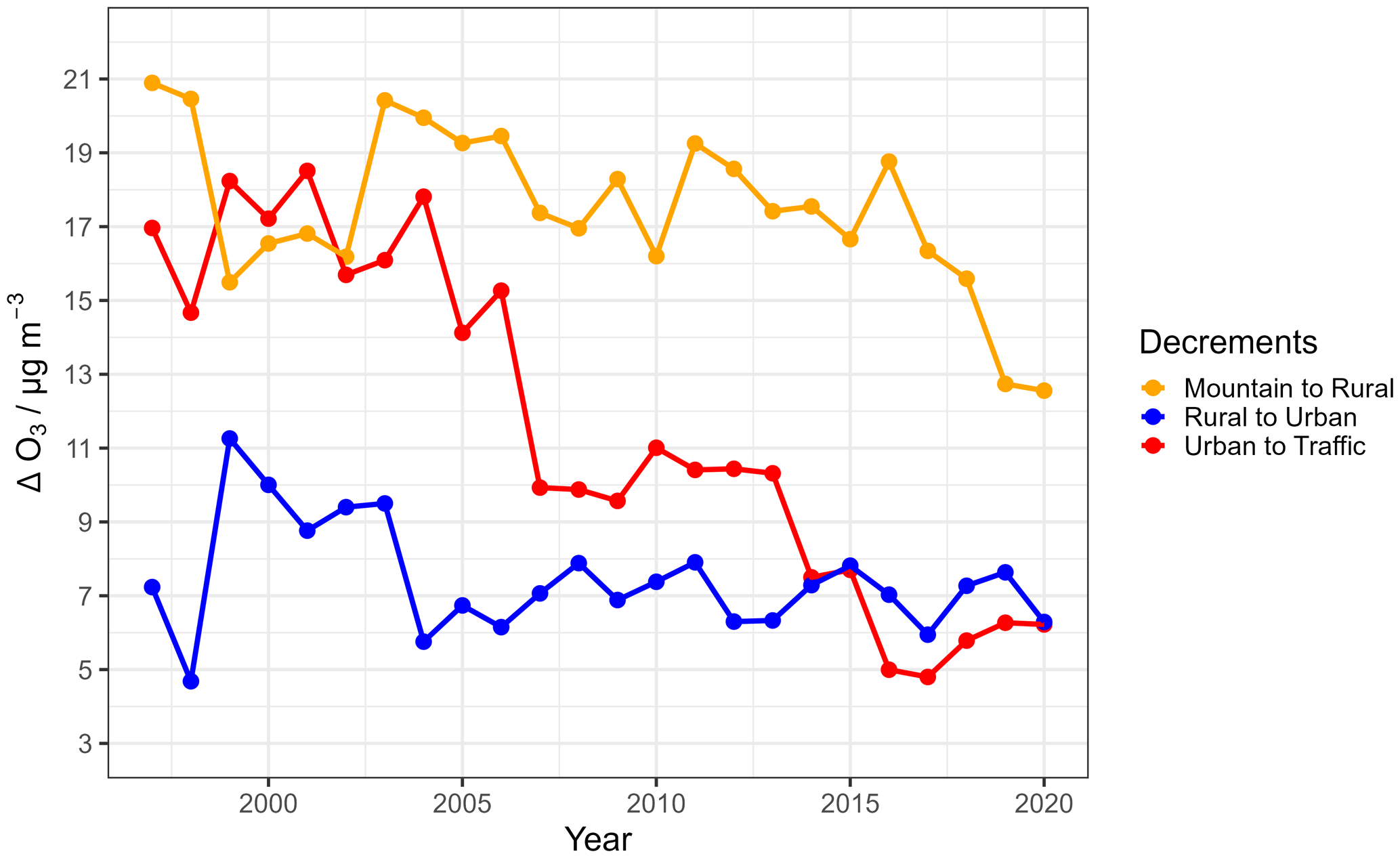
Figure 4 Mean yearly O₃ concentration differences, i.e. decrements, between different station types. Yellow lines with points represent decrements from mean mountain to mean rural station concentrations, blue lines with points represent rural to urban, and red lines with points represent urban to traffic station decrements.

It can be seen that the rural decrement, i.e. the concentration difference between the Ore Mountains stations and the rural background, decreased from about 15–21 µg m⁻³ at the turn of the century to values around 12 µg m⁻³ in more recent years. The urban decrement, i.e. rural to urban background difference, remained rather stagnant around 7 µg m⁻³ in all years except for the period 1999–2003. The traffic decrement from the urban background to the one long-term O₃ traffic station DD-Nord also decreased from about 15 to about 5–7 µg m⁻³ and is now at a similar level as the urban decrement. If the O₃ trends mentioned above continue in a similar way in the future, it can be expected that the typical O₃ concentrations at traffic stations will become more similar to those in the urban background, and rural background concentrations will become increasingly similar to those at the mountain sites. The Air Quality Expert Group (2021) reported a gradual convergence of urban and rural O₃ levels in the UK from 2000 to 2019, which is in contrast to the stable difference in O₃ concentration between urban and rural background observed since 2004 in the present study. The reason for this is the similarly increasing O₃ trends at urban and rural background sites in Saxony (Fig. 3), keeping the urban to rural decrement roughly similar. In any case, due to the typical settlement densities, these trends would mean higher O₃ exposures for the vast majority of the population.

One recent study by Yan et al. (2018), using a statistical trend model based on the data from 685 sites from the European Environment Agency Airbase system and 93 European rural background sites monitored by the Chemical Coordination Centre of the European Monitoring and Evaluation Programme (EMEP) network, has reported statistically significant growth rates of annual mean O₃ (0.20–0.59 µg m⁻³ yr⁻¹) in suburban and urban sites for the period 1995–2014, in contrast to a slight O₃ decrease from −0.09 to −0.02 µg m⁻³ yr⁻¹ (without clear statistical significance) over rural background sites. Despite the time period not being directly comparable, this is roughly similar to the trends observed in Saxony between 1997 and 2020, which averaged around 0.20 µg m⁻³ yr⁻¹ for urban background stations and close to zero for rural background stations. Further, Finch and Palmer (2020) reported that trends in annual mean O₃ in the UK over the period 1999–2019 were also rather stagnant at rural background stations, with a mean increase of 0.16 µg m⁻³ yr⁻¹ (not statistically significant), and slightly higher at urban background sites, with a mean increase of 0.47 µg m⁻³ yr⁻¹ (statistically significant), than the mean increase of 0.17 µg m⁻³ yr⁻¹ observed in the comparable 1997–2020 time period in the Saxony urban background. Other analyses of the UK O₃ trend over the period 2000 to 2019 (The Air Quality Expert Group, 2021) suggested that only moderate increases in annual mean O₃ were observed at rural background sites, with a mean of 0.11 µg m⁻³ yr⁻¹, which is roughly between the mean values in Saxony (quasi-zero and 0.25 µg m⁻³ yr⁻¹ for the periods from 1997 and from 2006 to 2020, respectively). In UK suburbs and urban areas, O₃ showed upwards trends, sometimes significantly, over the period considered in the study, with an average increase of about 0.26 µg m⁻³ yr⁻¹, which is also similar to the mean values at urban background stations in Saxony (0.17 and 0.27 µg m⁻³ yr⁻¹ over the last 24 and 15 years, respectively).

Despite all heterogeneity in detail, these comparisons suggest O₃ increases, especially in urban areas and, to a certain extent, also in the rural background not only in Saxony, but in many places in Germany and Europe. The determined increases in the range of a few tenths of µg m⁻³ yr⁻¹ are not very high compared to the typical O₃ concentrations of approximately 40–60 µg m⁻³ for urban and rural sites (as shown in Fig. 2), but they document O₃ still being a problem, at least with regard to chronic exposure, which has not been solved despite the successful reduction of various precursor compounds, and even tends to increase in the future. This conclusion is also supported by the stronger O₃ increases in more recent years identified in this study and by Sicard (2021) compared to the longer time periods often considered in other studies.

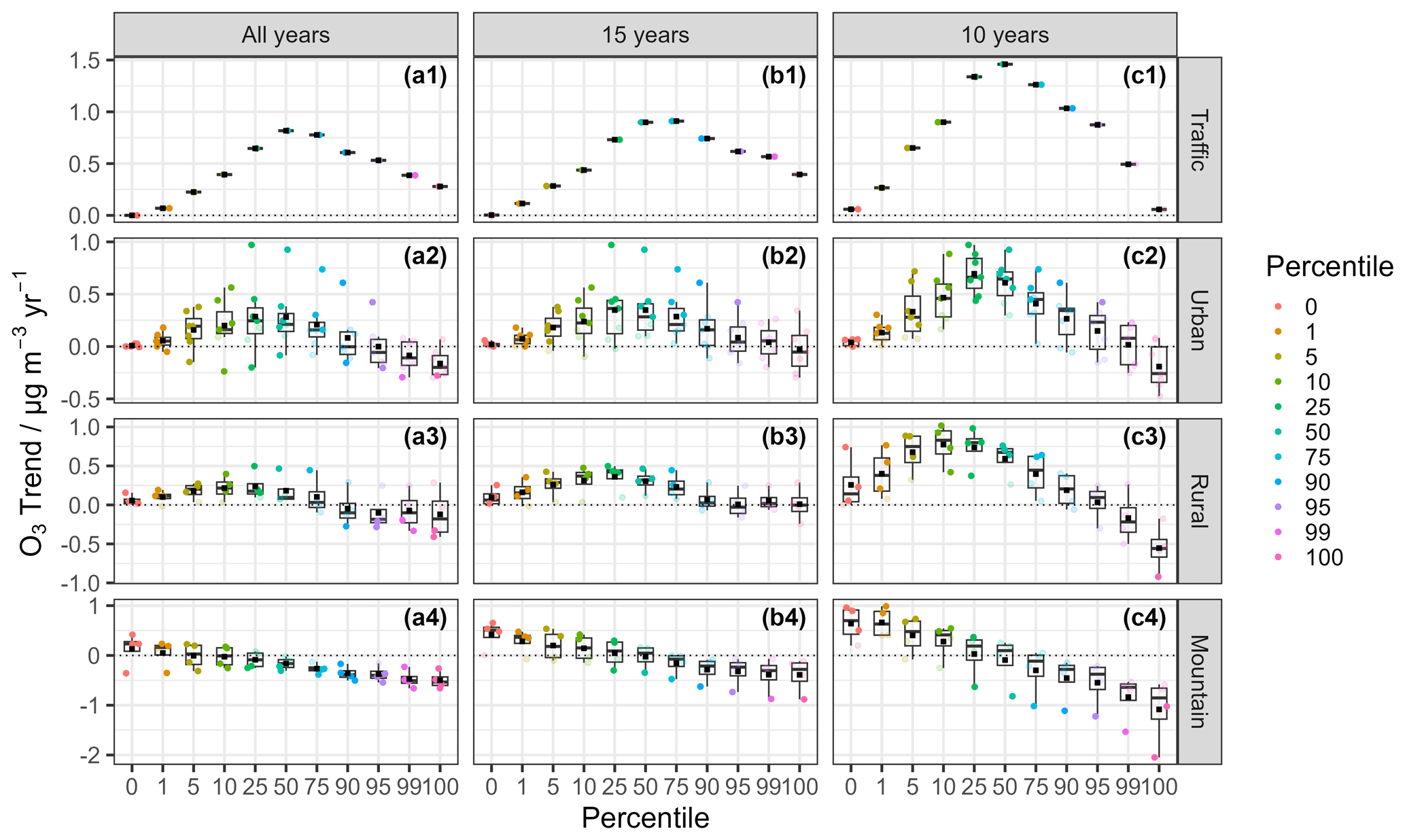
Figure 5 Theil–Sen trend values for different percentiles of O₃ concentrations for four station types (given in rows 1–4) and for three time periods until 2020 (given in columns a–c). Coloured dots show the values of individual stations, with solid dots for statistically significant trends and transparent dots otherwise. All dots are summarised by the box plots. The black square reflects the mean trend value per percentile.

3.1.3 Trends for different O₃ concentration levels

In addition to the trends of mean O₃ concentrations considered so far, it is interesting to also investigate concentration changes depending on the absolute O₃ concentrations. This can be achieved by calculating the trends of different O₃ percentiles. Low percentiles, i.e. 0, 1st, 5th and 10th, indicate the lowest and low concentration levels; medium percentiles, i.e. 25th, 50th and 75th, indicate middle concentration ranges; and high percentiles, i.e. 90th, 95th, 99th and 100th, indicate trends at high and the highest O₃ levels.

These trends over four station types within the three periods defined above are shown in Fig. 5.

Traffic site

The traffic-influenced site shows ozone increases for all concentrations (0–1.46 µg m⁻³ yr⁻¹) and the strongest trends at median concentrations around the 50th percentile combined with nearly no increases at the very low and very high percentiles. This behaviour led to the depicted bell-shaped curves. The longer the considered time frame, the smaller the dynamic range of the ozone trends from the median against more extreme concentration regimes. During the recent decade, the traffic site has exhibited the most pronounced increases across the entire concentration range.

Urban and rural background sites

For the urban and rural background there are quite similarly increasing trends (0–0.77 µg m⁻³ yr⁻¹) for nearly all concentration levels with the important exception that very high O₃ concentrations actually decrease (−0.55 to −0 µg m⁻³ yr⁻¹) and the strongest increases were seen already at the 10th and 25th percentiles, respectively, and not only at the 50th. Each O₃ concentration level has also shown a greater increase over the past decade or a more pronounced decrease at the highest concentrations compared to the other two periods. Additionally, the range of differences between peak values in the, again, bell-shaped curves during the recent decade is dampened against the traffic site and amounts to about 1 µg m⁻³ yr⁻¹.

Mountain sites

For all the mountain sites a monotonous decrease in the O₃ is seen with increasing concentration percentiles, and only for the smallest percentiles are O₃ increasing trends seen, which switch to O₃ decreasing trends at the 5th, 25th and 50th percentiles for all years, 15 years and 10 years, respectively. There is no bell shape anymore but a generally linear change.

Quantitatively, there are increases (0–0.66 µg m⁻³ yr⁻¹) in percentiles from the minimum to the 10th, turning into decreases (−1.08 to −0.28 µg m⁻³ yr⁻¹) in the higher percentiles (90–100th). The shorter the time frame considered, the more pronounced the stated trend.

Overall, during the recent 10 years, stagnant or even downward trends in the O₃ 90th, 95th, 99th and maximum in traffic, urban, rural and mountain stations occurred, while at the lower percentiles (minimum, 1st, 5th and 10th), O₃ concentrations across all stations seemingly continued to increase (with a mean trend ranging from 0.04–0.90 µg m⁻³ yr⁻¹). In the range of medium percentiles (from 25 to 75th), all traffic, urban and rural sites showed statistically significant increasing trends (ranging from 0.40 to 1.46 µg m⁻³ yr⁻¹), whilst at the mountain sites, they were decreasing or stagnant (−0.30–0.03 µg m⁻³ yr⁻¹).

Quite recently, Finch and Palmer (2020) similarly reported no statistically discernible decreasing trend (−0.49 µg m⁻³ yr⁻¹) in annual maximum O₃ on average, while mean concentrations and minimum concentrations increased at 0.41 and 0.09 µg m⁻³ yr⁻¹, respectively, across rural, suburban and urban background sites in the UK over the period 1999–2019. These findings can, at best, be compared to panels a2 and a3 of Fig. 5 in illustrating O₃ trends in a similar period from 1997–2020, with −0.15 µg m⁻³ yr⁻¹ for maximum O₃, 0.25 µg m⁻³ yr⁻¹ for median concentration and 0.03 µg m⁻³ yr⁻¹ at minimum concentration (as averaged values over panels a2 and a3 in Fig. 5). The results of another study in the UK (The Air Quality Expert Group, 2021) also revealed that the 50th and 25th percentile concentrations of O₃ clearly increased (from 0 to 0.94 µg m⁻³ yr⁻¹) at urban background sites over the period 2000–2019 (cf. panel a2 of Fig. 5 with 0.28–0.29 µg m⁻³ yr⁻¹ in a similar period from 1997–2020), whilst corresponding increases (from 0 to 0.66) at rural sites (cf. panel a3 of Fig. 5 with 0.18–0.24 µg m⁻³ yr⁻¹) are in general smaller (and in many cases not statistically significant). In addition, there have been stagnant or significant downward trends (−2.05 to 0.64 µg m⁻³ yr⁻¹, despite reported positive values are non-statistically significant) in the upper percentiles (99th and 99.9th percentiles) across all 27 sites examined, similar to our result of −0.16 to −0.07 µg m⁻³ yr⁻¹ in the 99th and 100th (as averaged values over panels a2 and a3 in Fig. 5).

Our results are consistent with previous analyses with negative or stagnant trends in the high range of percentiles (99–100th), indicative of fewer extreme O₃ episodes over time, which might be related to the reductions in NO_x, VOCs and CO emissions (Derwent et al., 2010; Yan et al., 2018, and references therein). The trends in lower and middle percentiles of O₃ are almost always positive, corresponding to the increasing baseline level of O₃ in the Northern Hemisphere (Jonson et al., 2006; Jenkin, 2008; Dentener et al., 2010; Cooper et al., 2014). Yan et al. (2018) used sensitivity simulations and statistical analysis to report that a decrease in European anthropogenic emissions lowered the 95th percentile of O₃ concentrations but enhanced the 5th percentile of O₃ in rural, suburban and urban sites during 1995–2014 over Europe. The results described here (decreasing trends in the higher range of percentiles – 95th–100th – of O₃ and increasing trends in the lower range of percentiles – 0th–5th – of O₃ as shown in Fig. 5a2–a4) may also reflect the effectiveness of emissions reductions in controlling the highest level of ozone for Saxony but also show an opposite effect at low concentration levels.

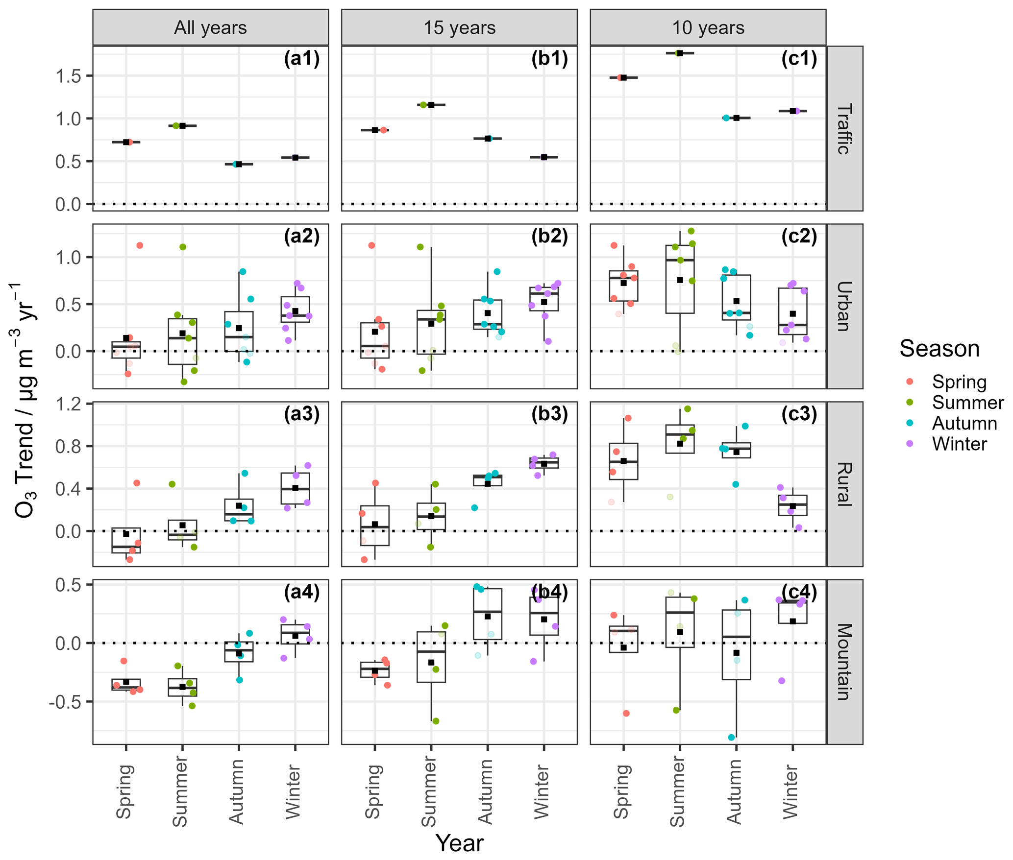
Figure 6 Theil–Sen trend values at different times of the year at the various station types (given in rows 1–4) and within each of the three time spans up to 2020 (given in columns a–c). Coloured dots show the values of individual stations, with solid dots for statistically significant trends and transparent dots otherwise. All dots are summarised by the box plots. The black square shows the mean trend value per season.

3.1.4 Trends in annual seasons

The mean trends by season at the different station types within the three time spans as used before are summarised in Fig. 6. For the traffic site, increasing trends are observed in all seasons over all time periods, but they are strongest in summer or spring of the latest period. In urban and rural background areas, a similar seasonal pattern was found for the recent 10 years, but for longer periods, spring and summer show lower increasing trends than autumn or winter. Particularly for mountain sites in spring and autumn, the trends during the longer periods are negative in contrast to the at least partly positive trends for the most recent decade. Yan et al. (2018) reported increasing trends (∼ 0.10 µg m⁻³ yr⁻¹) in winter mean O₃ and decreasing trends (∼ −0.30 µg m⁻³ yr⁻¹) in summer mean O₃ for the period 1995–2014 in suburban, urban and rural sites in Europe, which is similar to the trends observed here for all years (1997–2020); cf. Fig. 6 panels a2 and a3 at around 0.4 and 0.1 µg m⁻³ yr⁻¹ in winter and summer, respectively.

Gebhardt et al. (2021) also analysed a dataset of O₃ concentrations on the Ore Mountains ridge (Carlsfeld, Fichtelberg, Schwartenberg and Zinnwald) and found stagnating trends in the winters from 1997/98 to 2020, which is consistent with the result of mountain stations in this present study; see Fig. 6, panel a4.

3.2 Relationships between trends in O₃ and other measured trace gas concentrations and other parameters

In order to examine how the observed O₃ trends relate to the trends of other air pollutants, the trends for nitrogen oxides and the “oxidant” (O_x) as the sum of O₃ and NO₂ (Kley et al., 1994) are shown in Table S8 for the three time periods. Nitrogen oxides (NO, NO₂ and NO_x) show significantly decreasing trends since 1997 and over the last 10 years, consistent with reports that Europe-wide emissions of O₃ precursors (NO_x and other air pollutants) have decreased substantially since 1990 (Colette et al., 2015b; The Air Quality Expert Group, 2021). The MACCity inventory shows that anthropogenic NO_x emissions in Europe decreased by 35 % between 1995 and 2015 (Yan et al., 2018). This is comparable to the results identified here, which correspond to an average decrease of 31 % at all sites over the last decade (2011–2020). In addition, the inventories reported by the individual European countries can be found in the Air Pollutant Emissions Data Viewer (https://www.eea.europa.eu/data-and-maps/dashboards/air-pollutant-emissions-data-viewer-3, last access: 1 August 2025) of the European Environment Agency (EEA). This database shows that NO_x emissions in Germany decreased by about 31 % from 2011 to 2020, which is again consistent with the mean trends of nitrogen oxides reported here.

In addition to the directly measured air pollutants, it is useful to consider the trend of the so-called “oxidant” (O_x), which results from the sum of O₃ and NO₂ (Kley et al., 1994). In this way, the long-term change of the two oxidants can be better understood and evaluated, taking into account the effect of NO titration (NO + O₃= O₂+ NO₂) in the near-surface atmosphere.

Most stations in Saxony show stagnating or increasing O₃ (see Sect. 3.1), but Table S8D shows slightly decreasing O_x trends for all stations, which are, however, with the exception of the traffic station, only statistically significant for the longer period (≧15 years). The traffic station shows decreasing O_x trends of −0.26 µg m⁻³ yr⁻¹ during the last 10 years, which means that NO₂ has decreased slightly more than O₃ has increased. The O_x trend has tended to be stagnant (non-significant) over the 10 years at urban (−0.10 µg m⁻³ yr⁻¹), rural (−0.03 µg m⁻³ yr⁻¹) and mountain sites (−0.12 µg m⁻³ yr⁻¹), while similar decreasing trends as at the traffic station are observed for the longer period (∼ −0.20 µg m⁻³ yr⁻¹). At a busy road station in London, a local decrease in O_x of about 38 % over the period 2011–2020 was reported (The Air Quality Expert Group, 2021), which is significantly more than the decrease at the traffic site (DD-Nord) of about 0.68 % in the same period.

Overall, the O_x observations show that the increase in O₃ observed at some stations in Saxony is probably related to the decreasing NO_x. However, the stagnating O_x trends, especially in the more recent 10 years, show that the achieved emission reductions of the O₃ precursors obviously did not lead to sustainably and significantly lower O_x concentrations and thus to lower exposure to NO₂ and O₃ on average.

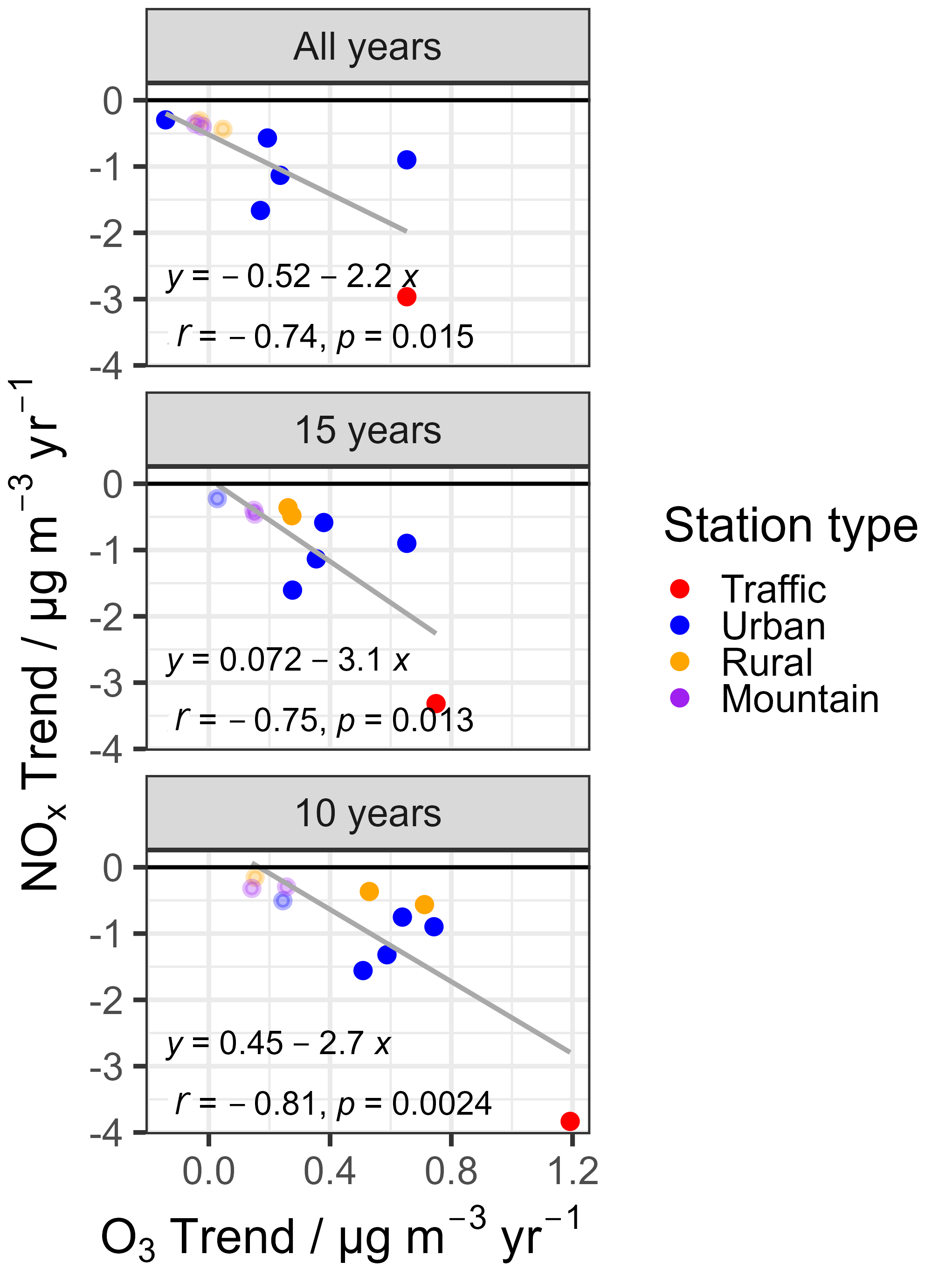
Figure 7 Relationships between O₃ trends and NO_x trends across all stations for the three different time periods (given in rows 1–3). Coloured dots show the values of individual stations, with solid dots for statistically significant O₃ trends and transparent dots otherwise. Also shown are linear fits for O₃ trends and NO_x trends in different time periods.

To understand the relationship between O₃ precursors and O₃ trends, the close chemical relationship between O₃ and the nitrogen oxides can be first investigated in Figs. 7 and S3 where the trends of NO_x, NO and NO₂ at all stations and for the different time periods are plotted above the respective trends of O₃ at the sites.

Regardless of the time period considered, it can be seen that the more the O₃ concentration at a station has been increasing, the more the nitrogen oxide concentrations have generally been decreasing. This pattern applies to all stations and is possibly a direct result of the classical Leighton chemistry, which describes how, during the day, a reduction in nitrogen oxide concentrations leads to a shift in the photostationary equilibrium towards higher O₃ concentrations. At night, lower NO_x concentrations mean a reduction in the sink strength of O₃ via the reaction with NO₂ and thus also higher resulting O₃ concentrations. In sum, the opposing trends of nitrogen oxides and O₃ trends result in the only very slightly decreasing and often stagnating trends of all O_x described above.

3.3 Photochemical model results

In Sect. 3.2 it has been found that there is a consistent increase in O₃ levels at monitoring stations, coupled with a noticeable decline in NO_x concentrations, particularly evident in many urban regions. Moreover, Figs. S4 and S5 show how the reduction in NO_x concentrations has correspondingly led to elevated O₃ levels across the four station types, both in summer and winter seasons spanning the period from 2000 to 2019. In this section, seasonal isopleths of O₃ formation will be diagnosed to offer insights into the controlling effects of NO_x and VOCs on O₃ variations across different station types throughout the 2000–2019 time frame. By visualising the station type-to-type variations within two seasonal isopleths (see Sect. 2.3 for detailed information), the present model-based analysis seeks to gauge the efficacy of precursor controls in Saxony over the past two decades and help shed some light on future mitigation strategies targeting O₃ pollution.

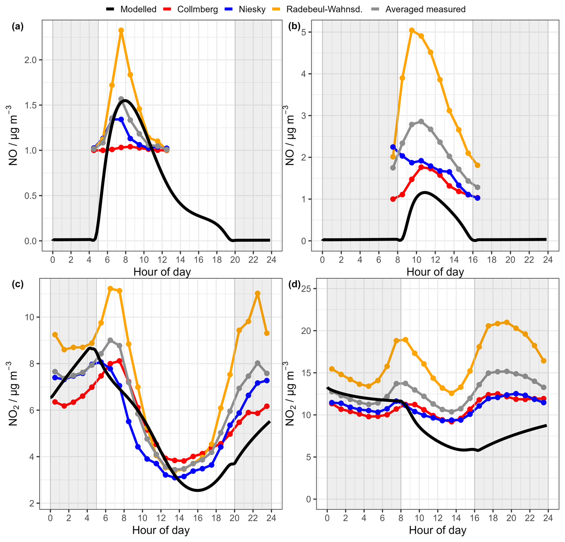
Figure 8 Diurnal profiles of hourly averaged modelled and observed NO and NO₂ in Saxony at rural background sites (panels a and c for the summer case; panels b and d for winter cases). Shaded areas indicate nighttime, black lines indicate the modelled values, grey lines represent averaged observed concentrations and coloured lines refer to the observed concentrations at each station. It is noted that all observed NO concentrations below the DL of 1 µg m⁻³ are not known and cannot be shown.

3.3.1 Simulation setup and comparison with 2019 measurements

As a first step in model development, the performance of the base case simulations for Saxony in 2019 was assessed. The year 2019 was chosen because of the best availability of the required input parameters. As a first set of results, the modelled NO and NO₂ diurnal patterns during summer and winter are compared with observed data at rural background stations in Fig. 8. It is noted that all measured NO concentrations below the detection limit (DL) of 1 µg m⁻³ are unknown and therefore not shown in the figure. Accordingly, the comparison of the NO patterns is only possible for hours with measured NO above the DL. The modelled NO concentrations during the period from 06:00 to 11:00 (CET) demonstrate satisfactory agreement with the observed summer data (Fig. 8a), with the exception of the most polluted Radebeul–Wahnsdorf site. During winter (Fig. 8b), the model seems to underpredict the NO concentrations, maybe because of a mixing layer being considered that is too high. However, the temporal pattern agrees rather well from 09:00–16:00 (CET). Therefore, the linear correlation coefficient (r) exceeds 0.8 from 06:00 to 11:00 in summer and remains above 0.7 from 09:00–16:00 (CET) in winter, indicating a robust correspondence between model outputs and measurements for both seasons. Additionally, the normalised mean bias factor (NMBF) (see its definition in the Supplement) (Jaidan et al., 2018) for model–measurement comparisons of NO is −0.03 during 06:00–11:00 in summer and −0.70 during 09:00–16:00 (CET) in winter, indicating satisfactory agreement of the model with mean measurements.

For NO₂ it can be seen that in summer (in Fig. 8c) the simulated NO₂ exhibits a 1 h earlier peak at 05:00 in the morning and a 1 h delay in the afternoon at 15:00. For all sites r between modelled and measured averaged NO₂ is at least 0.7. During the winter months, there is no correlation for the entire 24 h period, but it should be noted that at all sites it is above 0.7 during daytime hours, specifically between 08:00 and 15:00 (in Fig. 8d). Besides, NMBF values for model–measurement comparisons of NO₂ are −0.15 in summer and −0.29 in winter, indicating good agreement of the model with mean measurements. Overall, while the simulation captures the diurnal variations of NO and NO₂ reasonably well, a notable discrepancy partly persists between the simulated and observed concentration levels of NO_x. This inconsistency likely stems from the inherent uncertainties within the local emission inventory, particularly regarding the accurate estimation of local-site NO_x emission rates, or overestimation of the local mixing layer height also influencing the pollutant emissions rates.

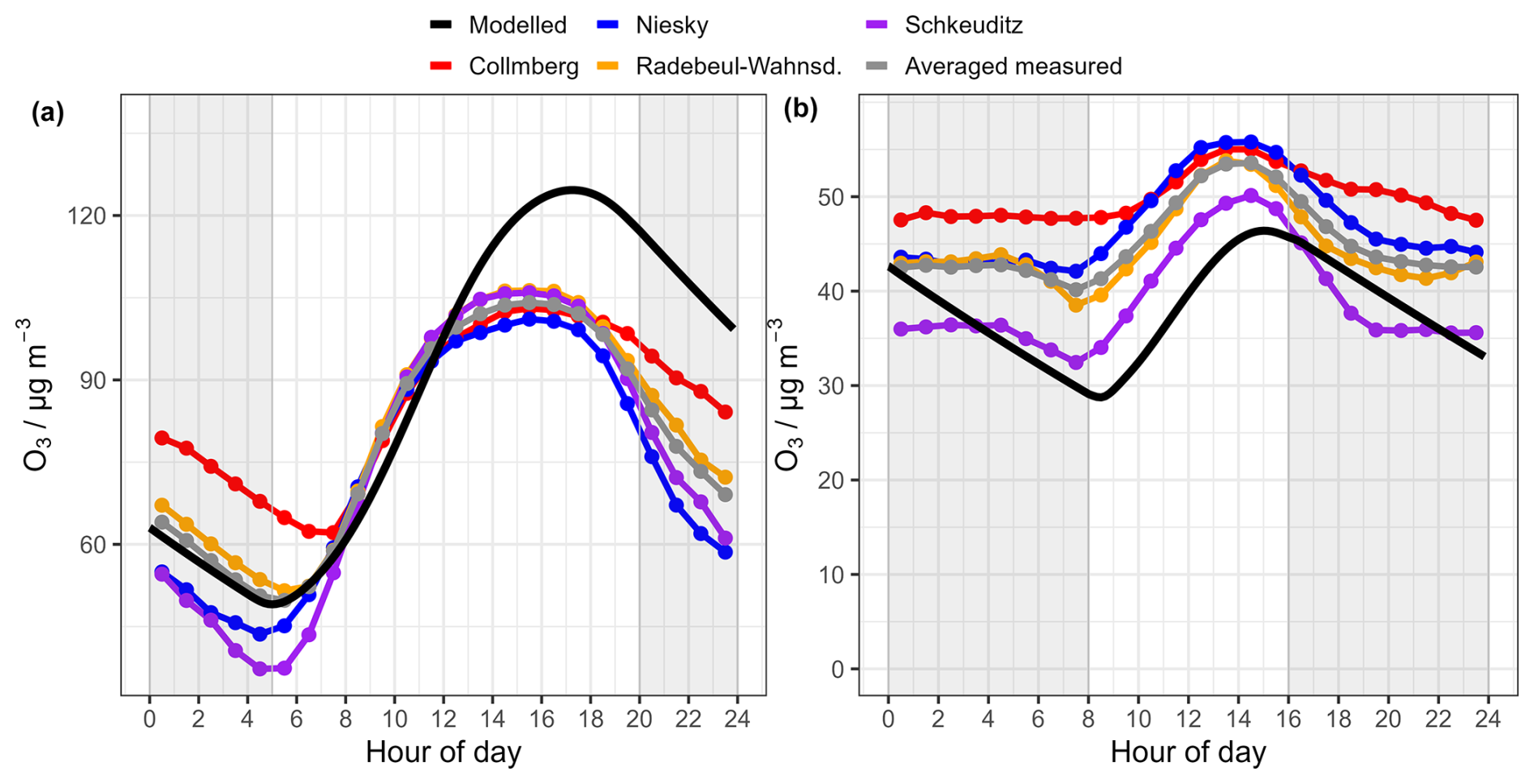
Figure 9 Diurnal profiles of hourly averaged modelled and observed O₃ in Saxony at rural background sites (a and b for summer and winter cases, respectively). Shaded areas indicate nighttime, black lines indicate the modelled O₃, grey lines represent averaged observed O₃ and other coloured lines refer to the observed O₃ at each station.

Figure 9 shows the diurnal profiles of hourly averaged simulated and observed O₃ concentrations during summer and winter. The model effectively reproduces both the magnitudes and diurnal patterns of observed O₃, demonstrating a strong correlation between observations and simulations (r>0.8). Additionally, NMBF values for model–measurement comparisons of O₃ are 0.12 in summer and −0.16 in winter, indicating good model performance. However, noteworthy exceptions include a higher simulated O₃ peak occurring after 13:00 and a 1 h delay in its occurrence. These deviations can be attributed to very localised near-site NO_x emissions (as depicted in Fig. 8), which cannot be adequately captured by the simulations.

Overall, Figs. 8 and 9 reveal reasonable agreement between the observed and simulated datasets. Therefore, the simulations were found to be generally able to reproduce the O₃ photochemistry for the conditions present in Saxony in 2019, enabling further sensitivity simulations of the O₃ and its characteristic dependencies on both the NO_x and VOC conditions.

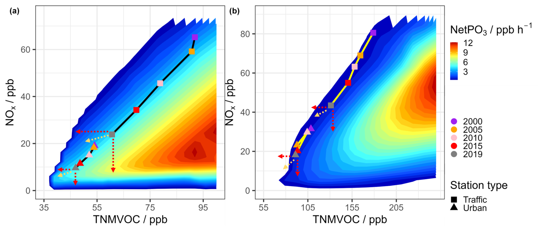
Figure 10 Isopleth plots for the net O₃ production rate (NetPO₃ in ppb h⁻¹) during 12:00–13:00 CET as a function of averaged NO_x and TNMVOC concentrations (a and b for summer and winter cases, respectively). NetPO₃ is shown using a rainbow colour scale. The coloured points represent the conditions in different years with squares showing traffic stations and triangles showing mean urban station conditions. The red dotted arrows represent hypothetical future scenarios with reductions in only one precursor (either TNMVOC or NO_x), while the yellow dotted arrows illustrate more plausible future pathways, where NetPO₃ slightly decreases through strong VOC emission controls combined with moderate NO_x reductions. Note that based on the underlying modelling, these data in Fig. 10 are given as mixing ratios. For better comparability with mass-based concentrations elsewhere in the paper, conversion factors of NO_x (µg m⁻³) $\approx \mathrm{1.5}\times$ NO_x (ppb) and O₃ (µg m⁻³) $\approx \mathrm{2}\times$ O₃ (ppb) can be used.

3.3.2 Isopleths for O₃ formation

Both Sect. 3.1 and Sect. 3.2 have highlighted a significant increase in O₃ levels in recent years. It is essential to elucidate the relationships between O₃ and its precursors in order to develop science-based control measures. Therefore, hundreds of sensitivity simulations were performed, incorporating various emission rate multipliers (outlined in Table S6) of TNMVOC and NO_x. These simulations of the base cases for Saxony (Sect. 3.3.1) aimed to elucidate the O₃ production rate with regards to the ambient concentrations of NO_x and TNMVOCs, which is depicted in the ozone isopleths of Fig. 10. A brief description of how these are produced is provided in Sect. 2.3. It can be seen that the diagrams resemble classic ozone isopleths typically produced with models (Sillman et al., 1990; Ehlers et al., 2016). They depict the in situ NetPO₃ as a function of NO_x and TNMVOC concentrations for both summer and winter scenarios.

In the next step, the measured values of NO_x and observed O₃ change rate (dO₃/dt) for the years 2000, 2005, 2010, 2015 and 2019 were used to indicate for each year the location in the isopleth diagram. A key challenge, however, was the lack of measured TNMVOC concentrations in all years. To work around this, three simulation batches (see Sect. 2.3 for details) were performed to achieve a sensible range of resulting TNMVOC and NO_x concentrations in the total of 800 and 1200 model runs for summer and winter, respectively. The point distribution of resulting TNMVOC and NO_x concentrations is shown in Fig. S6. Besides, the averaged NetPO₃ during noontime of 12:00–13:00 CET for each simulated scenario in both summer and winter conditions was obtained for each run. The resulting NetPO₃ was interpolated onto a regular 1000×1000 grid in the TNMVOC vs. NO_x space to generate Fig. S7. The O₃ isopleths (Fig. 10) were then fitted to this high-resolution grid from Fig. S7. At the same time, two tables present summer and winter data obtained after interpolation. From those, one can identify similar NO_x values along with their corresponding NetPO₃ and TNMVOC concentrations.

As depicted in Fig. S8, measured dO₃/dt and modelled NetPO₃ agreed reasonably well, particularly from 06:00 to 12:00 in summer and 08:00 to 12:00 in winter. This indicates that the measured dO₃/dt during these periods serves as a good proxy for the value of modelled NetPO₃, which is why it is considered valid to interchange them in the present application. By picking the known NO_x and dO₃/dt (finding the close values of NetPO₃), the TNMVOC concentration is then identified. For further clarification, in Tables S9 and S10, these TNMVOC estimates are shown together with a comparison of measured and modelled NO_x and dO₃/dt for the station types.

Notably, simulated TNMVOC concentrations, primarily emitted or locally photochemical in origin, are expected to be similar to or lower than previous measurements (Knobloch et al., 1997) because of lowered anthropogenic emissions through existing European regulations and corresponding mitigation measures. Indeed, unpublished data for a range of NMVOCs observed throughout the year 2022 in Borna, a city south of Leipzig, exhibited remarkably low concentrations of 66 NMVOC species (Table S11) at a near-road measurement site, with hourly mean and maximum total mixing ratios of 3.6 and 29.7 ppb in summer and 6.0 and 204.6 ppb in winter, respectively. Besides, von Schneidemesser et al. (2018) reported that the highest mixing ratios of a total of 57 NMVOC compounds measured during 3 summer months (June–August) at traffic sites in central and western Berlin were found to be 64 and 170 ppb, respectively. Thus, our estimated summer and winter TNMVOC concentrations (Tables S9 and S10) can be considered to lie in a reasonable range. However, for rural and mountain sites, accurate estimations for the TNMVOCs were challenging due to their very low NO_x concentrations (<10 ppb in summer, <16 ppb in winter) and dO₃/dt (<4 ppb h⁻¹ in summer, <1.3 ppb h⁻¹ in winter) observations (refer to Tables S9 and S10). Especially in the last 10 years, the data are near the lower-left border of simulated NO_x and NetPO₃ values in Fig. 10, where considerable uncertainty exists in estimating NetPO₃ and TNMVOCs. Therefore, only data for traffic and urban background sites are shown in Fig. 10.

The modelled NetPO₃ determined in the present study was in the range of 2.74 to 4.88 ppb h⁻¹ in summer (Table S9) and 0.78 to 1.65 ppb h⁻¹ in winter (Table S10) at traffic and urban sites between 2000 and 2019. In rural and mountain sites, the NetPO₃ is not given for the different years due to the uncertainty of the estimates, as described above. However, it can be said that measured dO₃/dt ranged from 1.16 to 3.89 ppb h⁻¹ in summer and 0.35 to1.30 ppb h⁻¹ in winter from 2000 to 2019. Modelled NetPO₃ and measured dO₃/dt were comparable to those deduced from other sites in Germany and Europe. For instance, Corsmeier et al. (2002) reported a NetPO₃ of 4.0–6.5 ppb h⁻¹ by a model system (KAMM/DRAIS) for a polluted ozone plume from Berlin during the July 1998 BERLIOZ campaign. In relatively clean rural and mountain sites, during the FREETEX'96 study at Mt. Jungfraujoch in April/May 1996, the NetPO₃ was calculated using a photochemical box model, yielding rates of 0.27 and 0.13 ppb h⁻¹ (Zanis et al., 2000), and Nussbaumer et al. (2021) reported a maximum midday NetPO₃ of 1.5 ppb h⁻¹ based on a photochemical calculation, considering in situ trace gas observations at a boreal forest site in Finland during the July and August 2010 HUMPPA campaign.

As can be seen from Fig. 10, O₃ photochemical formation in densely populated regions of Saxony is currently VOC-controlled and has also been VOC-controlled since the year 2000 in both summer and winter. In detail, for the summer case in Fig. 10a, traffic and urban background stations have a clear temporal trend and were in the VOC-limited regime overall from 2000 to 2019, but for the urban background stations the trend line in the recent 10 years is close to the transition regime (from VOC-limited to NO_x-limited regime). Detailed analyses (refer to Fig. 10a and Table S9) reveal a different trend line pattern in NetPO₃ between traffic and urban stations. At the traffic station, beginning at 2.74 ppb h⁻¹ in 2000, the NetPO₃ trend line crossed several isopleths, reaching 3.69 ppb h⁻¹ by 2005. Subsequently, it maintained a nearly parallel course with isopleths, starting with 3.87 ppb h⁻¹ in 2010 and then rising to 4.55 ppb h⁻¹ in 2019 over the recent decade. Concurrently, both NO_x and TNMVOC concentrations decreased by two-thirds and one-third, respectively. Conversely, urban background sites depict a slightly different scenario. An increase in NetPO₃, from 4.13 ppb h⁻¹ in 2000 to 4.87 ppb h⁻¹ in 2019 is noted within the isopleth plot. This rise occurred alongside substantial reductions in NO_x concentrations by 50 % (from 19.02 to 9.61 ppb), contrasting with only a small decrease in TNMVOC by approximately 15 % (54.06 to 46.91 ppb). Given that both traffic and urban sites are characterised by a VOC-limited regime, where NetPO₃ increases with decreasing ratios of NO_x $/$ TNMVOC, the observed increase in NetPO₃ and O₃ levels (as depicted in Fig. S9) confirms the inadequacy of current efforts of TNMVOC emission reductions with respect to O₃ pollution. Stronger reduction measures over the next years are needed, particularly in areas with dense population concentrations, to avoid exacerbating rather than mitigating ozone pollution.

In contrast to summer, winter experiences substantially weaker photochemistry, attributed to the lower intensity and shorter duration of solar radiation, which is merely half of that in summer. As illustrated in Fig. 10b and Table S10, traffic and urban background stations have exhibited relatively low NetPO₃ (<2.00 ppb h⁻¹) over the past two decades. Nevertheless, a slight increase in NetPO₃ has been observed (from approximately 0.80 in 2000 to about 1.60 ppb h⁻¹ in 2019 for traffic stations and from about 1.40 to roughly 1.60 ppb h⁻¹ for urban background sites, respectively), despite halving NO_x and TNMVOC emissions. Winter O₃ formation at both station types has predominantly occurred in the VOC-limited regime over the past 20 years, indicating that traffic and urban sites still have a considerable way to go in achieving NO_x-limited conditions despite significant NO_x emission controls. Additionally, it is worth noting that trend lines tend to run more parallel in the recent 5 or 10 years, irrespective of the season, suggesting that O₃ formation via photochemistry in densely populated regions under current emission controls has remained more consistent in recent years, contributing to O₃ increases (see Figs. S9 and S10).

As described above, NetPO₃ trends at rural and mountain sites could not be discussed using the modelled isopleths. Instead, trends in measured dO₃/dt are briefly discussed in the following. From summer 2000 to 2019, there was an increase in dO₃/dt by 1 and 0.5 ppb h⁻¹ (refer to Table S9) for rural and mountain sites, respectively. The rise in summer O₃ levels (refer to Fig. S9) may be attributed to an increase in photochemical production due to more on-site or transported O₃ precursors or an increase in the hemispheric background O₃ level due to elevated anthropogenic emissions in heavily polluted areas (Derwent et al., 2015; Gaudel et al., 2018; Mertens et al., 2020). The positive trends observed in the lower and middle percentiles of O₃ across all sites (see Fig. 5) in the present study further reinforce the assertion that background O₃ is rising. During winter from 2000 to 2019, rural sites experienced a slight increase in dO₃/dt by 0.2 ppb h⁻¹, while mountainous stations showed a decrease of −0.3 ppb h⁻¹ (refer to Table S10). Notably, winter O₃ trends increased at both sites, as depicted in Fig. S10, more likely due to the increase in the background O₃ level (Derwent et al., 2015; Gaudel et al., 2018; Mertens et al., 2020), as photochemistry has not changed significantly during the winters of the past 20 years.

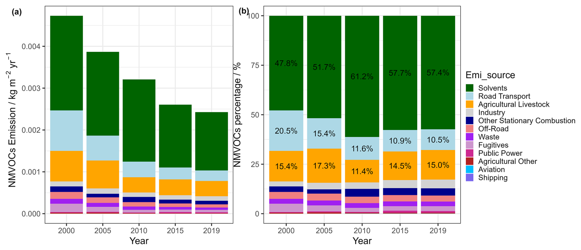
Figure 11 Anthropogenic emissions of NMVOCs in Saxony for 5 years between 2000 and 2019. Emission data were obtained by averaging values for each year across the approximated area of the entire state of Saxony (see Fig. S1). Details of the emission categories and corresponding emission sectors can be found in Table S13.

3.3.3 Implications for O₃ control

In the time frame of the present study, anthropogenic emissions of NMVOCs and NO_x have significantly decreased in the whole of Saxony (Figs. 11 and S11), as well as selected traffic (Figs. S12 and S13) and urban background areas (Figs. S14 and S15) over the last 20 years (from 2000 to 2019). Although the biogenic emissions data of year 2019 in overall Saxony (Fig. S16 and Table S12) are comparable to anthropogenic NMVOCs in the same year (Fig. 11a), biogenic emissions of isoprene and alpha-pinene in selected urban stations (Fig. S17 and Table S12) are indeed several orders of magnitude smaller than the anthropogenic emissions data in these areas (Fig. S14a). Limonene, on the other hand, cannot be regarded as solely biogenic but has important anthropogenic sources as well (Borbon et al., 2023; Gu et al., 2024). Thus, in urban sites it is inferred that biogenic emissions have a negligible effect on O₃ formation. The seasonal O₃ isopleths suggest that current O₃ formation regimes across traffic and urban background sites were determined to be overall VOC-limited during the same period. However, what kind of VOCs should be controlled to reach a more effective O₃ decrease is still uncertain. Based on the inventory data available for the present study (Fig. 11), it can be noted that the solvent emissions decreased less strongly than the total anthropogenic NMVOC emissions in Saxony, indicating an increased share of this emission category to regional O₃ formation. Similar changes in solvent emissions relative to total anthropogenic NMVOC emissions were also observed at traffic (Fig. S12) and urban background stations (Fig. S14). In fact, the percentage of solvent emissions in total anthropogenic NMVOC emissions remained nearly constant from 2010 to 2019, regardless of station types. This consistency suggests that solvent emissions may be a potential contributing factor to the increase in O₃ levels over the past decade. A recent study in the UK suggested an increased importance of solvents as well for summertime urban O₃ formation by incorporating detailed VOC emission inventories from 1990 to 2019 into a zero-dimensional chemical box model constrained by observational data (Li et al., 2024). Therefore, it is suggested that more strict VOC emission controls be implemented in the future, possibly with more attention to solvent use, in order to alleviate the O₃ pollution in Saxony.

However, a scenario that only reduces VOCs (as indicated by red dotted arrows to the left in Fig. 10) is not realistic as it comes with the cost of constant NO_x. Therefore, a scenario (as indicated by yellow dotted arrows in Fig. 10) where NetPO₃ slightly decreases, achieved through strong VOC emission control with a moderate NO_x emission decrease, is more realistic. In view of the detailed effect from diverse NMVOC emissions on O₃ pollution, more NMVOC measurements should be implemented to validate emission inventories and better refine modelling studies on O₃ formation.

4 Conclusions

Given the importance of surface ground-level O₃, long-term observations of O₃ concentrations are of utmost importance to understand the O₃ formation/depletion trend in a changing environment and climate. The present study compares the observed trends in O₃ concentrations across 16 measurement stations in Saxony, categorised into four station types (traffic, urban background, rural background and mountain sites) over three distinct periods: (i) the entire duration of available measurement data, from 1997 or later, (ii) the 15-year span from 2006 to 2020, and (iii) the more recent 10 years from 2011 to 2020. At 15 of the 16 measurement stations, surface O₃ exhibits upward or stagnant trends over the recent 15 or 10 years. The strongest O₃ trend is observed at the traffic DD-Nord station at roughly 1.2 µg m⁻³ yr⁻¹ (or 3.5 % yr⁻¹) in the last 10 years. Increasing O₃ trends are also observed at urban and rural background stations, with average rates of about 0.5 µg m⁻³ yr⁻¹ (or 1.1 % yr⁻¹) over the last decade. A more inhomogeneous picture can be seen on the mountain ridge, where over the last decade two stations (Schwartenberg and Zinnwald) have shown slightly positive but with not statistically significant O₃ trends. One station (Carlsfeld) was seen with a stagnating trend, and at the highest station of Fichtelberg the concentrations have clearly decreased at −0.79 µg m⁻³ yr⁻¹ (or −0.95 % yr⁻¹). In addition, ground-level NO_x measurements at these sites were analysed. Our results highlight that O₃ pollution in Saxony has not abated and has, in fact, worsened in the last 10 years, particularly in many urban areas with dense populations despite a reduction of NO_x concentrations at all sites. Through detailed photochemical modelling, isopleth plots for O₃ formation rates were constructed. Visualisation of year-to year variations per station type using two seasonal isopleth plots allows for assessing the effectiveness of precursor controls in Saxony over the past 20 years and offers insights into potential future O₃ pollution mitigation strategies.

It is shown that the O₃ formation dynamics across traffic and urban background sites were determined to be predominantly VOC-limited from 2000 to 2019. The observed increases in NetPO₃ and O₃ levels affirm that current efforts to reduce TNMVOC emissions from various sources are still insufficient. Continuing with a similar magnitude of VOC reductions in densely populated regions over the next years will likely result in further deterioration of O₃ pollution rather than its mitigation. Based on anthropogenic and biogenic emission data, we suggest that moderate NO_x reduction and additional VOC emission controls should be implemented, with particular attention given to solvent emissions, in order to more effectively alleviate regional O₃ formation. Given the detailed effects of various NMVOC emissions on O₃ increases and the complete lack of comprehensive NMVOC measurements, it is also strongly recommended to implement such monitoring. This would be of great help to assess emission inventories and improve the robustness of modelling studies on O₃ formation to develop prediction capability and undertake scenario calculations as to which path atmospheric ozone pollution will follow.