On the processes determining the slope of cloud water adjustments in weakly and non-precipitating stratocumulus

Cloud water adjustments are a part of aerosol–cloud interactions, affecting the ability of clouds to reflect solar shortwave radiation through processes altering the vertically integrated cloud water content L in response to changes in the droplet concentration N. In this study, we utilize a simple entrainment parameterization used in mixed-layer models to determine entrainment-mediated cloud water adjustments in weakly and non-precipitating stratocumulus. At lower N, L decreases due to an increase in entrainment in response to an increase in N suppressing the stabilizing effect of evaporating precipitation (virga) on boundary layer dynamics. At higher N, the decrease in cloud droplet sedimentation sustains more liquid water at the cloud top, and hence stronger preconditioning of free-tropospheric air, which increases entrainment with N. Using this idealized framework that neglects interactive surface fluxes, changes in boundary layer depth, and the diurnal cycle of solar radiation, we are able to show that cloud water adjustments weaken distinctly from $\mathrm{d}\ln \left(L\right)/\mathrm{d}\ln \left(N\right)=-\mathrm{0.48}$ at $N=\mathrm{100}{\mathrm{cm}}^{-\mathrm{3}}$ to −0.03 at $N=\mathrm{1000}{\mathrm{cm}}^{-\mathrm{3}}$, indicating that a single value to describe cloud water adjustments in weakly and non-precipitating clouds is insufficient. Based on these results, we speculate that cloud water adjustments at lower N are associated with slow changes in boundary layer dynamics, while a faster response is associated with the preconditioning of free-tropospheric air at higher N.

1 Introduction

By determining the concentration of cloud droplets N, aerosol has a substantial effect on the optical properties of clouds and their role in Earth's radiation budget (e.g., Boucher et al., 2013; Forster et al., 2021). While it is well known that an increase in N results in stronger reflection of incident solar shortwave radiation by increasing the number of scatterers (Twomey, 1974, 1977), further changes in the cloud micro- and macrostructure are less well understood. Concurrent changes in the vertically integrated cloud water content, the so-called liquid water path L, are especially important to consider, as they strengthen or weaken any impact of the aforementioned Twomey effect (e.g., Stevens and Feingold, 2009). These aerosol-mediated changes in L are referred to as cloud water adjustments and they are often quantified as

$$\begin{array}{}\text{(1)}& {\displaystyle }{\displaystyle }m\equiv {\displaystyle \frac{\mathrm{d}\ln \left(L\right)}{\mathrm{d}\ln \left(N\right)}}.\end{array}$$

m tends to be positive when an increase in N results in smaller cloud droplets, which suppress precipitation and increase L (Albrecht, 1989). In the absence of precipitation, further increases in N are found to increase the mixing of clouds with their surroundings (entrainment), leading to a decrease in L (Wang et al., 2003; Ackerman et al., 2004; Bretherton et al., 2007). Thus, m tends to be positive for precipitating clouds and negative for non-precipitating clouds (e.g., Gryspeerdt et al., 2019). While the m values at low and high N are likely related (Hoffmann et al., 2024b), the value of m in non-precipitating clouds is not understood, with most observational estimates ranging from −0.4 to −0.2 (e.g., Christensen and Stephens, 2011; Gryspeerdt et al., 2019; Possner et al., 2020), with a suggested lower limit of −0.64 (Glassmeier et al., 2021). Moreover, a single m to describe cloud water adjustments in non-precipitating stratocumulus might not be sufficient as m seems to be a function of N (e.g., Lu and Seinfeld, 2005; Chen et al., 2011).

Additionally, observational approaches to estimate m need to consider the natural variability in L due to, e.g., the diurnal cycle of solar radiation (e.g., Wood et al., 2002) and changes in the large-scale meteorological conditions (e.g., Chun et al., 2023; Goren et al., 2025). While models can be used to eliminate the influence of some of these confounding factors, the variability of m in weakly or non-precipitating clouds is likely associated with a complex network of interactions and dependencies that comprise entrainment (Mellado, 2017; Igel, 2024), making it hard to obtain direct process understanding even from models that represent the underlying dynamics explicitly, e.g., three-dimensional large-eddy simulations. Thus, to understand m for weakly and non-precipitating stratocumulus better, we will base our work on a simple, zero-dimensional mixed-layer model (Lilly, 1968; Schubert et al., 1979a; Bretherton and Wyant, 1997; Stevens, 2002). We will focus on the representation of the entrainment rate in such models and how it depends on L and N, which allows us to directly assess the individual aspects of the entrainment process (Nicholls and Turton, 1986; Turton and Nicholls, 1987; Bretherton et al., 2007). Despite this fundamentally simpler approach, our mixed-layer model results agree qualitatively with large-eddy simulations published in a companion paper (Chen et al., 2025).

The study is structured as follows. In Sect. 2, we will lay out the mathematical framework of the applied model, covering the fundamentals of the analyzed mixed-layer model entrainment parameterization and the approach to extract m from that parameterization. Results are presented in Sect. 3, and conclusions are drawn in Sect. 4.

2 Mathematical framework

2.1 Mixed-layer models

For mixed-layer models (e.g., Schubert et al., 1979a), it is a convenient choice to describe the boundary layer predicting the moist static energy as

$$\begin{array}{}\text{(2)}& {\displaystyle }{\displaystyle }s=c_{\mathrm{p}}T+gh+L_{\mathrm{v}}{q}_{\mathrm{v}},\end{array}$$

the total water mixing ratio as

$$\begin{array}{}\text{(3)}& {\displaystyle }{\displaystyle }{q}_{\mathrm{t}}=q_{\mathrm{v}}+q_{\mathrm{l}},\end{array}$$

and the boundary layer depth as

$$\begin{array}{}\text{(4)}& {\displaystyle }{\displaystyle }{h}_{\mathrm{t}}.\end{array}$$

Here, c_p is the specific heat capacity of air at constant pressure, T absolute temperature, g acceleration by gravity, h height above surface, L_v enthalpy of evaporation, q_v water vapor mixing ratio, and q_l liquid water mixing ratio.

Changes in s and q_t are determined by their respective fluxes from the surface, $\stackrel{\mathrm{‾}}{w^{\prime }{s}^{\prime }}{|}_{\mathrm{0}}$ and $\stackrel{\mathrm{‾}}{w^{\prime }{q}_{\mathrm{t}}^{\prime }}{|}_{\mathrm{0}}$, and the free troposphere, w_eΔs and w_eΔq_t, where w_e is the entrainment rate and Δs and Δq_t are the respective changes (jumps) of s and q_t from the mixed layer to the free troposphere. Further, s and q_t are affected by processes taking place inside the mixed layer, such as emission and absorption of radiation, affecting s, and precipitation, reducing q_t. h_t is determined by the interplay of w_e and subsidence w_s. Lastly, s, q_t, and h_t can change due to large-scale advection. In this study, however, we will solely focus on how w_e depends on L and N, which will give us an estimate of how entrainment affects cloud water adjustments.

2.2 Entrainment

The foundation of many w_e parameterizations is the scaling

$$\begin{array}{}\text{(5)}& {\displaystyle }{\displaystyle \frac{w_{\mathrm{e}}}{w_{\ast }}}\sim {\mathit{Ri}}^{-\mathrm{1}}\end{array}$$

by Turner (1973). This relationship states that w_e is proportional to a characteristic velocity of the flow, e.g., the convective velocity w_∗, with the constant of proportionality being determined by the inverse Richardson number:

$$\begin{array}{}\text{(6)}& {\displaystyle }{\displaystyle }{\mathit{Ri}}^{-\mathrm{1}}={\displaystyle \frac{w_{\ast }^{\mathrm{2}}}{h_{\mathrm{t}}\mathrm{\Delta }b}}.\end{array}$$

This scaling reflects the fact that the dynamics of the boundary layer, represented by w_∗, have to be sufficiently strong to overcome the stably stratified boundary layer top, represented by the buoyancy jump between the boundary layer and free troposphere Δb, to mix free-tropospheric air into the boundary layer. Typically, $w_{\ast }^{\mathrm{3}}$ is related to the vertically integrated buoyancy flux $h_{\mathrm{t}}\langle B\rangle ={\int }_{\mathrm{0}}^{h_{\mathrm{t}}}\stackrel{\mathrm{‾}}{w^{\prime }{b}^{\prime }}\left(h\right)\mathrm{d}h$ such that

$$\begin{array}{}\text{(7)}& {\displaystyle }{\displaystyle }{w}_{\ast }^{\mathrm{3}}=A{h}_{\mathrm{t}}\langle B\rangle ,\end{array}$$

with an efficiency factor A (Deardorff, 1976; vanZanten et al., 1999). Thus,

$$\begin{array}{}\text{(8)}& {\displaystyle }{\displaystyle }{w}_{\mathrm{e}}=A{\displaystyle \frac{\langle B\rangle }{\mathrm{\Delta }b}}.\end{array}$$

In the following, we will address how Δb, 〈B〉, and A are specified. Figure 1 shows all these contributions and the resulting w_e in an L–N phase space, with more detailed explanations following in Sect. 3.

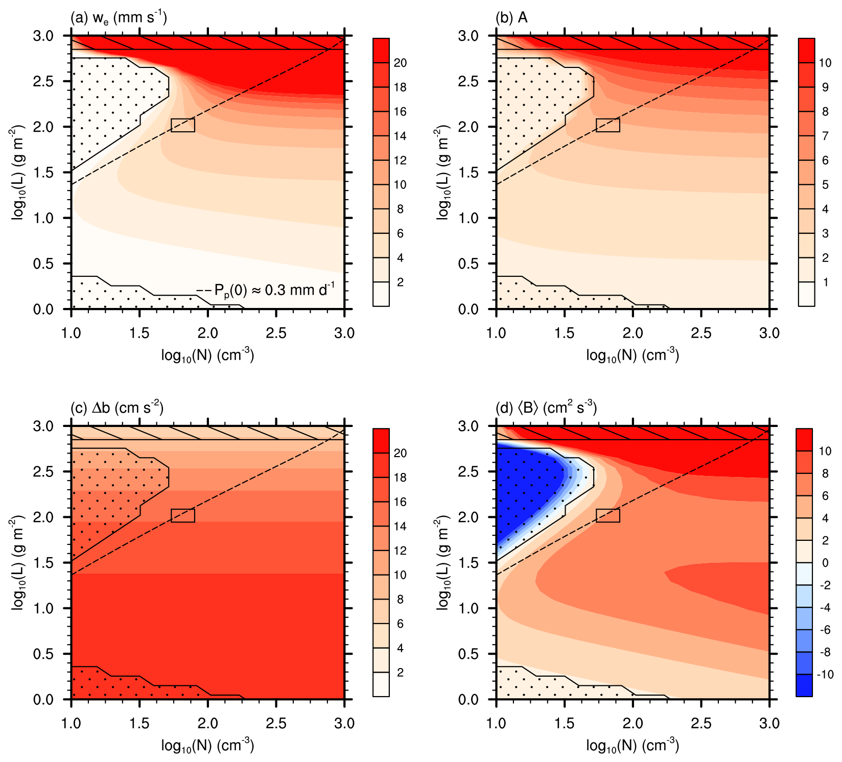
Figure 1 A representation of (a) the entrainment velocity w_e, (b) entrainment efficiency A, (c) buoyancy jump Δb, and (d) vertically averaged buoyancy flux 〈B〉 as a function of the liquid water path L and droplet number concentration N. Stippled regions denote decoupled boundary layers, while striped regions indicate that the cloud base is at or below the surface. These regions should not be analyzed. The dashed line indicates a surface precipitation rate of $P_{\mathrm{p}}\left(\mathrm{0}\right)=\mathrm{0.1}\stackrel{\mathrm{‾}}{w^{\prime }{q}_{\mathrm{t}}^{\prime }}{|}_{\mathrm{0}}{\mathit{\rho }}_{\mathrm{0}}\approx \mathrm{0.3}\mathrm{mm}{\mathrm{d}}^{-\mathrm{1}}$, separating precipitating (to the left) from weakly and non-precipitating (to the right) parts of the phase space. The black rectangle indicates the L–N range observed during the second research flight of the DYCOMS-II campaign, as reported in Ackerman et al. (2009).

2.2.1 The buoyancy jump Δb

Following Schubert et al. (1979a), we define the virtual static energy as

$$\begin{array}{ll}{\displaystyle }{s}_{\mathrm{v}}& {\displaystyle }=s-L_{\mathrm{v}}{q}_{\mathrm{v}}+c_{\mathrm{p}}{T}_{\mathrm{0}}(\mathit{\eta }{q}_{\mathrm{v}}-q_{\mathrm{l}})\\ \text{(9)}& {\displaystyle }& {\displaystyle }=s-(\mathrm{1}-\mathit{\eta }\mathit{ϵ})L_{\mathrm{v}}{q}_{\mathrm{t}}+[\mathrm{1}-(\mathrm{1}+\mathit{\eta }\left)\mathit{ϵ}\right]L_{\mathrm{v}}{q}_{\mathrm{l}},\end{array}$$

with the definitions $\mathit{ϵ}=\left(c_{\mathrm{p}}{T}_{\mathrm{0}}\right)/L_{\mathrm{v}}$ and $\mathit{\eta }=R_{\mathrm{v}}/R_{\mathrm{d}}-\mathrm{1}$, with R_v and R_d the specific gas constants of water vapor and dry air, respectively, and T₀ a reference temperature. Thus, the buoyancy of a parcel of air is

$$\begin{array}{}\text{(10)}& {\displaystyle }{\displaystyle }b={\displaystyle \frac{g}{T_{\mathrm{0}}{c}_{\mathrm{p}}}}{s}_{\mathrm{v}},\end{array}$$

and the buoyancy jump between the top of the boundary layer to the free troposphere is

$$\begin{array}{ll}{\displaystyle }\mathrm{\Delta }b& {\displaystyle }=b(h_{\mathrm{t}}+\mathit{\delta }h)-b\left(h_{\mathrm{t}}\right)\\ {\displaystyle }& {\displaystyle }={\displaystyle \frac{g}{T_{\mathrm{0}}{c}_{\mathrm{p}}}}\mathit{\{}\mathrm{\Delta }s-\left(\mathrm{1}-\mathit{\eta }\mathit{ϵ}\right)L_{\mathrm{v}}\mathrm{\Delta }{q}_{\mathrm{t}}\\ \text{(11)}& {\displaystyle }& {\displaystyle }-\left[\mathrm{1}-\left(\mathrm{1}+\mathit{\eta }\right)\mathit{ϵ}\right]L_{\mathrm{v}}{q}_{\mathrm{l}}\left(h_{\mathrm{t}}\right)\mathit{\}},\end{array}$$

where δh is a height difference (assumed to be small) from the boundary layer top to the free troposphere, defining the aforementioned jumps $\mathrm{\Delta }s=s(h_{\mathrm{t}}+\mathit{\delta }h)-s\left(h_{\mathrm{t}}\right)$ and $\mathrm{\Delta }{q}_{\mathrm{t}}=q_{\mathrm{t}}(h_{\mathrm{t}}+\mathit{\delta }h)-q_{\mathrm{t}}\left(h_{\mathrm{t}}\right)$. Note that the free-tropospheric $q_{\mathrm{l}}(h_{\mathrm{t}}+\mathit{\delta }h)=\mathrm{0}$ per definition.

2.2.2 The average buoyancy flux 〈B〉

The dynamics of the stratocumulus-topped boundary layer are primarily driven by buoyancy, and the corresponding buoyancy flux can be expressed as

$$\begin{array}{ll}{\displaystyle }\stackrel{\mathrm{‾}}{w^{\prime }{b}^{\prime }}\left(h\right)& {\displaystyle }={\displaystyle \frac{g}{T_{\mathrm{0}}{c}_{\mathrm{p}}}}\stackrel{\mathrm{‾}}{w^{\prime }{s}_{\mathrm{v}}^{\prime }}\left(h\right)\\ \text{(12)}& {\displaystyle }& {\displaystyle }={\displaystyle \frac{g}{T_{\mathrm{0}}{c}_{\mathrm{p}}}}\left[{\mathit{\alpha }}_{\mathrm{s}}\left(h\right)\stackrel{\mathrm{‾}}{w^{\prime }{s}^{\prime }}\left(h\right)-{\mathit{\alpha }}_{q_{\mathrm{t}}}\left(h\right)L_{\mathrm{v}}\stackrel{\mathrm{‾}}{w^{\prime }{q}_{\mathrm{t}}^{\prime }}\left(h\right)\right],\end{array}$$

where the coefficients

$$\begin{array}{}\text{(13)}& {\displaystyle }{\displaystyle }{\mathit{\alpha }}_{\mathrm{s}}\left(h\right)=\left\{\begin{array}{ll}\mathrm{1}& \text{for }h<h_{\mathrm{b}},\\ \mathit{\beta }& \text{for }h>h_{\mathrm{b}},\end{array}\right.\end{array}$$

and

$$\begin{array}{}\text{(14)}& {\displaystyle }{\displaystyle }{\mathit{\alpha }}_{q_{\mathrm{t}}}\left(h\right)=\left\{\begin{array}{ll}\mathrm{1}-\mathit{\eta }\mathit{ϵ}& \text{for }h<h_{\mathrm{b}},\\ \mathit{ϵ}& \text{for }h>h_{\mathrm{b}},\end{array}\right.\end{array}$$

represent changes in the buoyancy flux due to latent heat release above cloud base h_b. Thus, they vary for subsaturated or saturated conditions, i.e., below and above cloud base, respectively. Here, $\mathit{\beta }=[\mathrm{1}+\mathit{\gamma }\mathit{ϵ}(\mathit{\eta }+\mathrm{1}\left)\right]/[\mathrm{1}+\mathit{\gamma }]$ considers the change in s due to condensation or evaporation, with $\mathit{\gamma }=(L_{\mathrm{v}}/c_{\mathrm{p}}){\left.\mathrm{d}{q}_{\mathrm{s}}/\mathrm{d}T\right|}_{{\mathrm{p}}_{\mathrm{0}}}$ representing the change in the saturation water vapor mixing ratio q_s with T, commonly referred to the Clausius–Clapeyron relation. Typically, β≈0.5, $\mathrm{1}-\mathit{\eta }\mathit{ϵ}\approx \mathrm{0.9}$, and ϵ≈0.1, indicating that the influence of $\stackrel{\mathrm{‾}}{w^{\prime }{s}^{\prime }}$ and $\stackrel{\mathrm{‾}}{w^{\prime }{q}_{\mathrm{t}}^{\prime }}$ on $\stackrel{\mathrm{‾}}{w^{\prime }{b}^{\prime }}$ changes from below to above cloud base.

Under well-mixed conditions, contributions to the buoyancy flux that originate from the surface or the top of the boundary layer can be assumed to increase or decrease linearly within the boundary layer, reaching zero at the opposite side of the boundary layer (e.g., Bretherton and Wyant, 1997). Thus, the surface buoyancy flux can be expressed as

$$\begin{array}{ll}{\displaystyle }{\left.\stackrel{\mathrm{‾}}{w^{\prime }{b}^{\prime }}\right|}_{\mathrm{0}}\left(h\right)=& {\displaystyle \frac{g}{T_{\mathrm{0}}{c}_{\mathrm{p}}}}\left[{\mathit{\alpha }}_{\mathrm{s}}\left(h\right){\left.\stackrel{\mathrm{‾}}{w^{\prime }{s}^{\prime }}\right|}_{\mathrm{0}}-{\mathit{\alpha }}_{q_{\mathrm{t}}}\left(h\right)L_{\mathrm{v}}{\left.\stackrel{\mathrm{‾}}{w^{\prime }{q}_{\mathrm{t}}^{\prime }}\right|}_{\mathrm{0}}\right]\\ \text{(15)}& {\displaystyle }& {\displaystyle }\times \left(\mathrm{1}-{\displaystyle \frac{h}{h_{\mathrm{t}}}}\right).\end{array}$$

Similarly, the entrainment buoyancy flux from the layer's top yields

$$\begin{array}{ll}{\displaystyle }{\left.\stackrel{\mathrm{‾}}{w^{\prime }{b}^{\prime }}\right|}_{\mathrm{e}}\left(h\right)=& {\displaystyle \frac{g}{T_{\mathrm{0}}{c}_{\mathrm{p}}}}\left[-{\mathit{\alpha }}_{\mathrm{s}}\left(h\right)w_{\mathrm{e}}\mathrm{\Delta }s+{\mathit{\alpha }}_{q_{\mathrm{t}}}\left(h\right)L_{\mathrm{v}}{w}_{\mathrm{e}}\mathrm{\Delta }{q}_{\mathrm{t}}\right]\\ \text{(16)}& {\displaystyle }& {\displaystyle }\times \left({\displaystyle \frac{h}{h_{\mathrm{t}}}}\right).\end{array}$$

The effect of longwave radiation cooling is represented as

$$\begin{array}{}\text{(17)}& {\displaystyle }{\displaystyle }{\left.\stackrel{\mathrm{‾}}{w^{\prime }{b}^{\prime }}\right|}_{\mathrm{r}}\left(h\right)={\displaystyle \frac{g}{T_{\mathrm{0}}{c}_{\mathrm{p}}}}\left[{\mathit{\alpha }}_{\mathrm{s}}\left(h\right)\mathrm{\Delta }{F}_{\mathrm{r}}{\mathit{\rho }}_{\mathrm{0}}\right]\left({\displaystyle \frac{h}{h_{\mathrm{t}}}}\right),\end{array}$$

which is confined to the top of the boundary layer, where longwave radiative cooling takes place primarily. Similar to Dal Gesso et al. (2014), we express the longwave radiative cooling rate as

$$\begin{array}{ll}{\displaystyle }\mathrm{\Delta }{F}_{\mathrm{r}}& {\displaystyle }=F_{\mathrm{r}}\left(h_{\mathrm{t}}\right)-F_{\mathrm{r}}\left(\mathrm{0}\right)\\ \text{(18)}& {\displaystyle }& {\displaystyle }=\mathrm{\Delta }{F}_{\text{r,}\ast }\left[\mathrm{1}-\exp (-{\mathit{\kappa }}_{\mathrm{r}}L)\right]-{\mathit{\lambda }}_{\mathrm{r}}\ln \left[b_{\mathrm{r}}\right(q_{\text{t,0}}+\mathrm{\Delta }{q}_{\mathrm{t}}\left)\right],\end{array}$$

where the first term on the right-hand side describes the radiative cooling across the boundary layer, which is scaled by $\left[\mathrm{1}-\exp (-{\mathit{\kappa }}_{\mathrm{r}}L)\right]$ to consider the saturation of longwave radiative cooling toward larger L (e.g., Stephens, 1978). Here, κ_r, is the effective emissivity. The second term of Eq. (18) represents the effect of free-tropospheric moisture, warming the cloud top. $\mathrm{\Delta }{F}_{\text{r,}\ast }=\mathrm{88.2}\mathrm{W}{\mathrm{m}}^{-\mathrm{2}}$, ${\mathit{\lambda }}_{\mathrm{r}}=\mathrm{16.5}\mathrm{W}{\mathrm{m}}^{-\mathrm{2}}$, and b_r=1000 have been determined from fitting ΔF_r against the free-tropospheric q_t using an ensemble of stratocumulus large-eddy simulations that employed a detailed radiative transfer code. The underlying data are shown in Fig. 9a of Chen et al. (2024). Note that κ_r is a function of the (effective) droplet radius at cloud top r_l(h_t) and is determined by fitting the values stated in Table 1 of Larson et al. (2007). Moreover, it is assumed that all cooling is concentrated at the cloud top. Thus, Eq. (17) cannot represent the N effect on the spatial distribution of longwave radiative cooling and hence entrainment, as recently discussed by Igel (2024). Similar to our companion paper (Chen et al., 2025), we neglect interactions with solar radiation for simplicity.

Based on Bretherton et al. (2007), we include the effect of droplet sedimentation as

$$\begin{array}{}\text{(19)}& {\displaystyle }{\displaystyle }{\left.\stackrel{\mathrm{‾}}{w^{\prime }{b}^{\prime }}\right|}_{\mathrm{s}}\left(h\right)=-g{P}_{\mathrm{s}}\left(h\right),\end{array}$$

where the liquid water flux by sedimentation is expressed as

$$\begin{array}{}\text{(20)}& {\displaystyle }{\displaystyle }{P}_{\mathrm{s}}\left(h\right)=\left\{\begin{array}{ll}\mathrm{0}& \text{for }h<h_{\mathrm{b}},\\ w_{\mathrm{t}}\left(h\right)q_{\mathrm{l}}\left(h\right)& \text{for }h>h_{\mathrm{b}},\end{array}\right.\end{array}$$

with the terminal velocity of the sedimenting droplets given by $w_{\mathrm{t}}\left(h\right)=k_{\mathrm{t}}{r}_{\mathrm{l}}^{\mathrm{2}}\left(h\right)$, and $k_{\mathrm{t}}=\mathrm{1.19}\times {\mathrm{10}}^{\mathrm{8}}{\mathrm{m}}^{-\mathrm{1}}{\mathrm{s}}^{-\mathrm{1}}$ (Rogers and Yau, 1989). Note that sedimenting droplets are assumed to be small enough that they do not fall below cloud base.

As we will show below, the complete evaporation of precipitation falling below cloud base (virga) can have a substantial impact on the boundary layer dynamics of weakly precipitating clouds. This effect is expressed as

$$\begin{array}{ll}{\displaystyle }{\left.\stackrel{\mathrm{‾}}{w^{\prime }{b}^{\prime }}\right|}_{\mathrm{p}}\left(h\right)=& {\displaystyle \frac{g}{T_{\mathrm{0}}{c}_{\mathrm{p}}}}{\mathit{\alpha }}_{q_{\mathrm{t}}}\left(h\right)L_{\mathrm{v}}\\ \text{(21)}& {\displaystyle }& {\displaystyle }\times \left[P_{\mathrm{p}}\left(h\right)-P_{\mathrm{p}}\left(\mathrm{0}\right)\left(\mathrm{1}-{\displaystyle \frac{h}{h_{\mathrm{t}}}}\right)\right].\end{array}$$

The precipitation liquid water flux is determined as

$$\begin{array}{}\text{(22)}& {\displaystyle }{P}_{\mathrm{p}}\left(h\right)=\left\{\begin{array}{ll}{P}_{\mathrm{p}}\left(h_{\mathrm{b}}\right)-\left[P_{\mathrm{p}}\left(h_{\mathrm{b}}\right)-P_{\mathrm{p}}\left(\mathrm{0}\right)\right]\frac{h_{\mathrm{b}}-h}{h_{\mathrm{b}}}& \text{for }h<h_{\mathrm{b}},\\ P_{\mathrm{p}}\left(h_{\mathrm{b}}\right)\left(\mathrm{1}-\frac{h-h_{\mathrm{b}}}{h_{\mathrm{l}}}\right)& \text{for }h>h_{\mathrm{b}},\end{array}\right.\end{array}$$

bounded by its cloud-base and surface values $P_{\mathrm{p}}\left(h_{\mathrm{b}}\right)=k_{\mathrm{p}}(L/N{)}^{\mathrm{1.75}}$ and $P_{\mathrm{p}}\left(\mathrm{0}\right)=P_{\mathrm{p}}\left(h_{\mathrm{b}}\right)\exp \left[-(h_{\mathrm{b}}/h_{\mathrm{p}}{)}^{\mathrm{1.5}}\right]$, respectively, with $k_{\mathrm{p}}=\mathrm{2.44}\times {\mathrm{10}}^{\mathrm{10}}{\mathrm{kg}}^{-\mathrm{0.75}}{\mathrm{m}}^{-\mathrm{3.75}}{\mathrm{s}}^{-\mathrm{1}}$ and h_p=475 m from Wood (2007) and the geometrical cloud depth defined as

$$\begin{array}{}\text{(23)}& {\displaystyle }{\displaystyle }{h}_{\mathrm{l}}=h_{\mathrm{t}}-h_{\mathrm{b}}.\end{array}$$

Note that there are different expressions for P_p(h_b) and its dependency on N and L discussed in the literature (e.g., Kostinski, 2008; Feingold et al., 2013), opening the potential for slight quantitative changes in the results.

The boundary-layer-averaged buoyancy flux is determined from its individual components as

$$\begin{array}{ll}{\displaystyle }\langle B\rangle & {\displaystyle }={\displaystyle \frac{\mathrm{1}}{h_{\mathrm{t}}}}\underset{\mathrm{0}}{\overset{h_{\mathrm{t}}}{\int }}\stackrel{\mathrm{‾}}{w^{\prime }{b}^{\prime }}\left(h\right)\mathrm{d}h\\ {\displaystyle }& {\displaystyle }={\displaystyle \frac{\mathrm{1}}{h_{\mathrm{t}}}}\underset{\mathrm{0}}{\overset{h_{\mathrm{t}}}{\int }}\sum _i{\left.\stackrel{\mathrm{‾}}{w^{\prime }{b}^{\prime }}\right|}_i\left(h\right)\mathrm{d}h\\ \text{(24)}& {\displaystyle }& {\displaystyle }=\sum _i\langle B{\rangle }_i,\end{array}$$

where all contributions to $\stackrel{\mathrm{‾}}{w^{\prime }{b}^{\prime }}$ are integrated analytically.

Note that 〈B〉|_r, 〈B〉|_s, and 〈B〉|_p directly depend on N, while 〈B〉|_e exhibits an indirect dependency since w_e depends on 〈B〉 and hence all aforementioned direct dependencies. Moreover, to avoid the recursive dependency of w_e on w_e via 〈B〉|_e, many parameterizations rearrange Eq. (8) to solve for w_e directly. However, such parameterizations impede the understanding of the basic dependencies of w_e (see Stevens, 2002). Thus, we solve Eq. (8) iteratively. All contributions to 〈B〉 are presented in an L–N phase space in Fig. 2a–e and will be analyzed in more detail in Sect. 3.

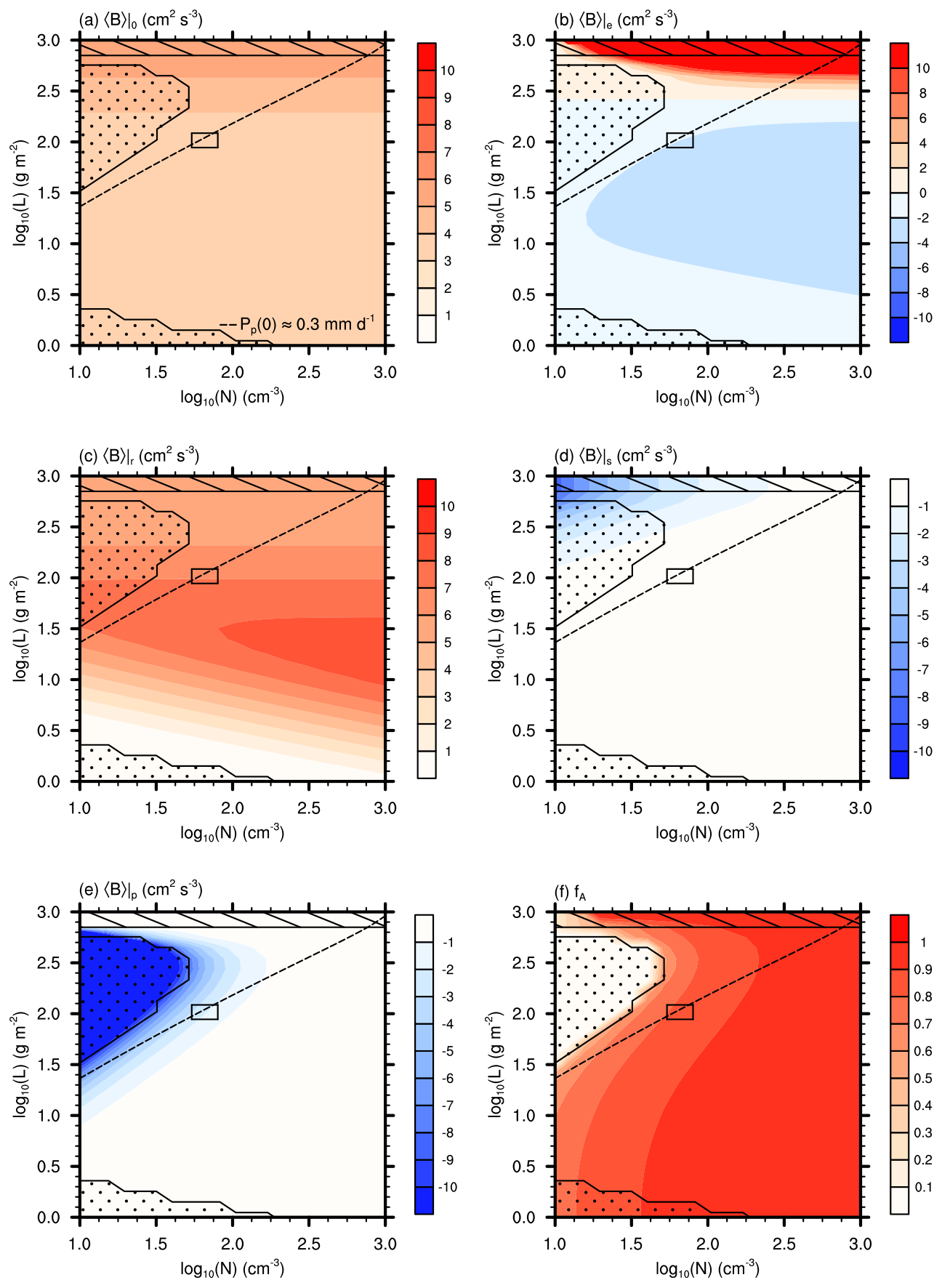
Figure 2 A representation of (a) the vertically averaged surface buoyancy flux 〈B〉|₀, (b) entrainment buoyancy flux 〈B〉|_e, (c) longwave radiation buoyancy flux 〈B〉|_r, (d) sedimentation buoyancy flux 〈B〉|_s, (e) precipitation buoyancy flux 〈B〉|_p, and (f) sedimentation–entrainment feedback parameterization f_A as a function of the liquid water path L and droplet number concentration N. See Fig. 1 for further explanations.

2.2.3 The efficiency factor A

Based on the seminal work by Nicholls and Turton (1986) and Turton and Nicholls (1987), the entrainment efficiency can be expressed as

$$\begin{array}{}\text{(25)}& {\displaystyle }{\displaystyle }A={\displaystyle \frac{\mathrm{2}{a}_{\text{A,1}}}{\mathrm{1}-a_{\text{A,1}}}}\left[\mathrm{1}+a_{\text{A,2}}{\mathit{\chi }}_{\mathrm{A}}\left(\mathrm{1}-{\displaystyle \frac{\mathit{\delta }{b}_{\mathrm{A}}}{\mathrm{\Delta }b}}\right)f_{\mathrm{A}}\right],\end{array}$$

where a_A,1=0.2 is recommended for representing entrainment in dry boundary layers (Deardorff, 1976), for which the bracketed term is neglected. The bracketed term represents the increase in entrainment due to the presence of liquid water at the cloud top. Yamaguchi and Randall (2012) have shown that the evaporation of liquid water mixed with free-tropospheric air cools and hence decreases the positive buoyancy of the free-tropospheric air, facilitating its subsequent entrainment. The minimum buoyancy of a mixture of boundary layer and free-tropospheric air is achieved when all liquid water is evaporated and the mixture is exactly saturated (Stevens, 2002). Grenier and Bretherton (2001) showed that this buoyancy is

$$\begin{array}{}\text{(26)}& {\displaystyle }{\displaystyle }\mathit{\delta }{b}_{\mathrm{A}}={\displaystyle \frac{g}{T_{\mathrm{0}}{c}_{\mathrm{p}}}}(\mathit{\beta }\mathrm{\Delta }s-\mathit{ϵ}{L}_{\mathrm{v}}\mathrm{\Delta }{q}_{\mathrm{t}}),\end{array}$$

with

$$\begin{array}{}\text{(27)}& {\displaystyle }{\displaystyle }{\mathit{\chi }}_{\mathrm{A}}=-{\displaystyle \frac{q_{\mathrm{l}}\left(h_{\mathrm{t}}\right)/\mathrm{\Delta }{q}_{\mathrm{t}}}{\mathrm{1}-\frac{\mathit{\gamma }}{\mathrm{1}+\mathit{\gamma }}\frac{\mathrm{\Delta }s}{L_{\mathrm{v}}\mathrm{\Delta }{q}_{\mathrm{t}}}}}\end{array}$$

being the necessary mass fraction of free-tropospheric air to evaporate all liquid water in this mixture. Note that other approaches to determine δb_A and χ_A exist, e.g., the average over all possible mixtures (e.g., Dal Gesso et al., 2014). Further, the parameter a_A,2=15 is used in this study, as recommended by Bretherton et al. (2007), while Nicholls and Turton (1986) suggest 60.

Lastly, Bretherton et al. (2007) introduced f_A in the bracketed term of Eq. (25) to represent the removal of liquid water from the cloud top by droplet sedimentation, thereby decreasing the potential for evaporative cooling and hence entrainment. At the same time, f_A considers convection to replenish the liquid water. To combine these effects, Bretherton et al. (2007) suggested

$$\begin{array}{}\text{(28)}& {\displaystyle }{\displaystyle }{f}_{\mathrm{A}}=\exp \left[-a_{\text{A,3}}{\displaystyle \frac{w_{\mathrm{t}}\left(h_{\mathrm{t}}\right)}{w_{\ast }}}\right],\end{array}$$

where a_A,3=9 is a fitting parameter and $w_{\mathrm{t}}\left(h_{\mathrm{t}}\right)=k_{\mathrm{t}}{r}_{\mathrm{l}}^{\mathrm{2}}\left(h_{\mathrm{t}}\right)$. Thus, f_A causes the bracketed term in Eq. (25) to approach 1 when sedimentation is strong (w_t→∞) or convection weak ($w_{\ast }\to \mathrm{0}$).

Note that we do not include an evaporation–entrainment feedback to describe N-dependent evaporation at the cloud top (e.g., Wang et al., 2003; Igel, 2024). While no parameterization for this effect exists, it is reasonable to assume that it should behave similarly to the sedimentation–entrainment feedback described by Eq. (28). Thus, increasing the magnitude of a_A,3 in Eq. (28) can be seen as a means to estimate the effect of evaporation–entrainment and is done in Sect. 3.3.

2.3 Determining cloud water adjustments

2.3.1 Relations to L and N

To understand cloud water adjustments due to entrainment, we would like to express w_e as a function of L and N. We start by determining q_l as a function of the distance to the cloud base h_b, i.e.,

$$\begin{array}{}\text{(29)}& {\displaystyle }{\displaystyle }{q}_{\mathrm{l}}\left(h\right)=\left\{\begin{array}{ll}\mathrm{0}& \text{for }h<h_{\mathrm{b}},\\ {\mathrm{\Gamma }}_{\mathrm{l}}(h-h_{\mathrm{b}})& \text{for }h>h_{\mathrm{b}},\end{array}\right.\end{array}$$

where Γ_l describes the increase in liquid water mixing ratio with height (e.g., Albrecht et al., 1990). Thus,

$$\begin{array}{}\text{(30)}& {\displaystyle }{\displaystyle }L=\underset{\mathrm{0}}{\overset{h_{\mathrm{t}}}{\int }}{\mathit{\rho }}_{\mathrm{0}}{q}_{\mathrm{l}}\left(h\right)\mathrm{d}h={\displaystyle \frac{\mathrm{1}}{\mathrm{2}}}{\mathit{\rho }}_{\mathrm{0}}{\mathrm{\Gamma }}_{\mathrm{l}}{h}_{\mathrm{l}}^{\mathrm{2}},\end{array}$$

using Eq. (23) and the reference air density ρ₀. This definition allows us to express h_l as

$$\begin{array}{}\text{(31)}& {\displaystyle }{\displaystyle }{h}_{\mathrm{l}}={\left({\displaystyle \frac{\mathrm{2}L}{{\mathit{\rho }}_{\mathrm{0}}{\mathrm{\Gamma }}_{\mathrm{l}}}}\right)}^{\mathrm{1}/\mathrm{2}}\end{array}$$

and the corresponding cloud-top value of q_l as

$$\begin{array}{}\text{(32)}& {\displaystyle }{\displaystyle }{q}_{\mathrm{l}}\left(h_{\mathrm{t}}\right)={\mathrm{\Gamma }}_{\mathrm{l}}{h}_{\mathrm{l}}={\left({\displaystyle \frac{\mathrm{2}{\mathrm{\Gamma }}_{\mathrm{l}}L}{{\mathit{\rho }}_{\mathrm{0}}}}\right)}^{\mathrm{1}/\mathrm{2}}.\end{array}$$

The droplet radius changes with h as

$$\begin{array}{}\text{(33)}& {\displaystyle }{\displaystyle }{r}_{\mathrm{l}}\left(h\right)={\left[{\displaystyle \frac{q_{\mathrm{l}}\left(h\right){\mathit{\rho }}_{\mathrm{0}}}{\frac{\mathrm{4}}{\mathrm{3}}\mathit{\pi }{\mathit{\rho }}_{\mathrm{l}}N}}\right]}^{\mathrm{1}/\mathrm{3}},\end{array}$$

and the corresponding cloud-top value is

$$\begin{array}{}\text{(34)}& {\displaystyle }{\displaystyle }{r}_{\mathrm{l}}\left(h_{\mathrm{t}}\right)={\left({\displaystyle \frac{\mathrm{9}{\mathrm{\Gamma }}_{\mathrm{l}}L{\mathit{\rho }}_{\mathrm{0}}}{\mathrm{8}{\mathit{\pi }}^{\mathrm{2}}{\mathit{\rho }}_{\mathrm{l}}^{\mathrm{2}}{N}^{\mathrm{2}}}}\right)}^{\mathrm{1}/\mathrm{6}}.\end{array}$$

By prescribing L and N, as well as the parameters h_t, T₀, and ρ₀, Eqs. (31)–(34) can be used to express Δb, 〈B〉, A, and hence w_e as a function of L and N. Thus, s and q_t are not required to determine Δb, 〈B〉, A, and w_e but are assumed to adjust such that a prescribed value of L is obtained.

2.3.2 Base assumptions

The large-eddy simulations in our companion paper (Chen et al., 2025) show that a positive perturbation of N, δN>0, results in an increase in w_e in response to an aerosol perturbation (see their Fig. 4a). After sufficient time (18 h), this increase in w_e is diminished, resulting in negligible differences in w_e among the perturbed and unperturbed simulations. This decrease in w_e is enabled by a commensurate decrease in L in the perturbed simulations, δL<0, resulting in increasingly stronger negative m with time (see their Fig. 2c). Note that other parameters assumed to be constant in our framework (e.g., h_t) change insignificantly among the perturbed and unperturbed simulations (see their Fig. 4b). We approximate this late-stage behavior by

$$\begin{array}{}\text{(35)}& {\displaystyle }{\displaystyle }{w}_{\mathrm{e}}(N,L)=w_{\mathrm{e}}(N+\mathit{\delta }N,L+\mathit{\delta }L).\end{array}$$

Using the mixed-layer model entrainment parameterization w_e outlined above, Eq. (35) is solved iteratively for δL using prescribed values of L, N, and δN, while keeping all other parameters constant (e.g., surface fluxes, boundary layer depth). Then, cloud water adjustments are quantified as $m\approx \left[\ln (L+\mathit{\delta }L)-\ln \left(L\right)\right]/\left[\ln (N+\mathit{\delta }N)-\ln \left(N\right)\right]$.

Note that Eq. (35) describes a condition that is assumed to be valid in addition to other changes affecting L and N. Since Eq. (35) is only valid after sufficient time has elapsed (18 h) (Chen et al., 2025), stratocumulus that exhibit faster changes in L and N should not be assessed using Eq. (35). This might be the case for stratocumulus that are far from their steady-state L (Hoffmann et al., 2020, 2024b; Glassmeier et al., 2021). On the other hand, slower processes that affect h_t or L on longer timescales do not influence our assessment (Schubert et al., 1979b; Stevens, 2006; Bretherton et al., 2010). Additionally, Eq. (35) does not consider adjustments in surface fluxes (Bretherton and Wyant, 1997), as well as the impact of solar radiation (Chen et al., 2024), for which more complex models would be required. Nonetheless, the large-eddy simulations presented in our companion paper (Chen et al., 2025) indicate that sufficient physics are captured in Eq. (35) to yield reasonable insights, as we will detail below.

Moreover, it is important to reiterate that the m determined from Eq. (35) is only valid for stratocumulus-topped boundary layers that are driven by the interplay of entrainment and longwave radiation (Hoffmann et al., 2020), with a negligible contribution of surface precipitation. Surface precipitation would constitute a loss term for L that is not considered in Eq. (35). Thus, m should only be interpreted for parts of the L–N phase space where losses by surface precipitation are negligible. Positive m values, traditionally associated with precipitation suppression (e.g., Albrecht, 1989), are not part of our solution.

2.4 Parameters

The default stratocumulus-topped boundary layer analyzed here is based on the large-eddy simulation intercomparison case by Ackerman et al. (2009), derived from the second research flight of the DYCOMS-II campaign that focused on subtropical stratocumulus off the coast of California (Stevens et al., 2003). Here, we use their surface fluxes $\stackrel{\mathrm{‾}}{w^{\prime }{q}_{\mathrm{t}}^{\prime }}{|}_{\mathrm{0}}=\mathrm{93}\mathrm{W}{\mathrm{m}}^{-\mathrm{2}}/\left(L_{\mathrm{v}}{\mathit{\rho }}_{\mathrm{0}}\right)$ and $\stackrel{\mathrm{‾}}{w^{\prime }{s}^{\prime }}{|}_{\mathrm{0}}=\mathrm{16}\mathrm{W}{\mathrm{m}}^{-\mathrm{2}}/{\mathit{\rho }}_{\mathrm{0}}+L_{\mathrm{v}}\stackrel{\mathrm{‾}}{w^{\prime }{q}_{\mathrm{t}}^{\prime }}{|}_{\mathrm{0}}=\mathrm{109}\mathrm{W}{\mathrm{m}}^{-\mathrm{2}}/{\mathit{\rho }}_{\mathrm{0}}$, jumps $\mathrm{\Delta }{q}_{\mathrm{t}}=-\mathrm{4.45}\mathrm{g}{\mathrm{kg}}^{-\mathrm{1}}$ and $\mathrm{\Delta }s/c_{\mathrm{p}}=\mathrm{6.7}\mathrm{K}+\mathrm{\Delta }{q}_{\mathrm{t}}{L}_{\mathrm{v}}/c_{\mathrm{p}}\approx -\mathrm{3.3}\mathrm{K}$, and boundary layer depth h_t=795 m, unless otherwise noted. To estimate the free-tropospheric humidity for determining the effect of longwave radiative cooling (Eq. 18), we prescribe $q_{\text{t,0}}=\mathrm{9.45}\mathrm{g}{\mathrm{kg}}^{-\mathrm{1}}$ based on the initial values of Ackerman et al. (2009). Note that this q_t,0 is not used anywhere else in our framework. Other reference parameters are T₀=288.3 K, ${\mathit{\rho }}_{\mathrm{0}}=\mathrm{1.21}\mathrm{kg}{\mathrm{m}}^{-\mathrm{3}}$, and ${\mathrm{\Gamma }}_{\mathrm{l}}=\mathrm{2}\mathrm{g}{\mathrm{kg}}^{-\mathrm{1}}{\mathrm{km}}^{-\mathrm{1}}$.

Figures 1 and 2 contain black rectangles that indicate the L–N range observed during the second research flight of the DYCOMS-II campaign (Ackerman et al., 2009). The w_e determined from Eq. (8) agrees very well with the observed range of 6–8 mm s⁻¹ (see Ackerman et al., 2009). Additionally, 〈B〉 (Fig. 1d) and the surface precipitation rate P_p(0) (dashed lines in Figs. 1 and 2) are in general agreement with the values reported from the large-eddy simulation intercomparison by Ackerman et al. (2009). This indicates that the framework applied in this study reproduces the behavior of observed stratocumulus at least in some parts of the analyzed phase space.

3 Results

Most plots of this study show the L–N phase space, overlaid by different lines and patterns. The stippling marks potentially decoupled boundary layers, where the buoyancy flux is too weak to ensure a well-mixed boundary layer. These regions have been determined using the approach by Turton and Nicholls (1987), which diagnoses decoupling if the ratio of the integrated sub-cloud-layer buoyancy flux to the integrated cloud-layer buoyancy flux is smaller than −0.4. Reasons for the decoupling will be discussed more deeply when addressing 〈B〉. As decoupled boundary layers violate many assumptions reasonable for well-mixed boundary layers, this part of the phase space should not be assessed. Moreover, the striped part of the phase space marks regions where the cloud base is at or below the surface (h_b<0), and results should be disregarded. In fact, all $L>\mathrm{150}\mathrm{g}{\mathrm{m}}^{-\mathrm{2}}$ values are rather untypical for stratocumulus (Wood, 2012), and results in this part of the phase space should be analyzed with care. Since our approach does not consider losses in L due to surface precipitation, we neglect regions of the L–N phase space that are substantially affected by this process. The dashed line marks the surface precipitation rate $P_{\mathrm{p}}\left(\mathrm{0}\right)=\mathrm{0.1}\stackrel{\mathrm{‾}}{w^{\prime }{q}_{\mathrm{t}}^{\prime }}{|}_{\mathrm{0}}{\mathit{\rho }}_{\mathrm{0}}\approx \mathrm{0.3}\mathrm{mm}{\mathrm{d}}^{-\mathrm{1}}$. By determining this value based on $\stackrel{\mathrm{‾}}{w^{\prime }{q}_{\mathrm{t}}^{\prime }}{|}_{\mathrm{0}}$, we identify regions of the L–N phase space in which precipitation losses are substantial (to the left of the dashed line) and the region where precipitation losses are negligible, i.e., the weakly and non-precipitating clouds that are the main focus of this study (to the right of the dashed line). Note that the precipitation rate to discriminate these regions is comparable to the cloud-base precipitation rate of 0.5 mm d⁻¹ suggested by Wood (2012).

3.1 Entrainment at high N

Figure 1a shows w_e as a function of L and N. First, we address w_e in the non-precipitating part of the phase space between N=300 and 1000 cm⁻³, i.e., sufficiently far away from the precipitating phase space. Here, we see a strong increase in w_e with L, accompanied by a weak dependency on N. The strong increase in w_e with L can be attributed to a decrease in Δb (Fig. 1c) and an increase in A (Fig. 1b). The decrease in Δb is due to the stronger latent heat release at higher L, which decreases the temperature difference relative to the warmer free troposphere, as indicated by Eq. (11), enabling stronger entrainment. Note that Δb does not depend on N. The increase in A with L is primarily due to the larger amount of liquid water at the cloud top, requiring a much larger fraction of free-tropospheric air to be mixed with cloudy air to evaporate it according to Eq. (27), thus allowing more free-tropospheric air to be entrained into the boundary layer. For a given N, this effect is somewhat offset by the sedimentation–entrainment feedback (Eq. 28) (Fig. 2f), where an increase in droplet size with L increases the removal of liquid water from the cloud top by sedimentation, which decreases entrainment. Interestingly, the sedimentation–entrainment feedback decreases for sufficiently high L. This is because the sedimentation–entrainment feedback is proportional to $w_{\mathrm{t}}/w_{\ast }$, and the increase in w_∗ for $L>\mathrm{300}\mathrm{g}{\mathrm{m}}^{-\mathrm{2}}$ (see $\langle B\rangle \sim w_{\ast }^{\mathrm{3}}$ in Fig. 1d) outpaces the simultaneous increase in w_t. The slight increase in A with N is due to the weakening of the sedimentation–entrainment feedback for higher N, where decreasing droplet sedimentation from the cloud top enables stronger entrainment.

While 〈B〉 also affects w_e, its variability between N=300 and 1000 cm⁻³ is much weaker than the variability in Δb and A. Nonetheless, for $L<\mathrm{30}\mathrm{g}{\mathrm{m}}^{-\mathrm{2}}$, 〈B〉 exhibits a strong increase with L due to increasing longwave radiative cooling accelerating boundary layer dynamics, as shown by 〈B〉|_r (Fig. 2c). Note that the increase in longwave radiative cooling quickly saturates for $L>\mathrm{30}\mathrm{g}{\mathrm{m}}^{-\mathrm{2}}$ (Garrett et al., 2002). However, 〈B〉|_r decreases slightly after reaching a maximum at around $L=\mathrm{30}\mathrm{g}{\mathrm{m}}^{-\mathrm{2}}$. The coefficient in Eq. (13) and Eq. (17) indicates that $\stackrel{\mathrm{‾}}{w^{\prime }{b}^{\prime }}{|}_{\mathrm{r}}$ is smaller in saturated layers than in subsaturated ones. Because h_t is kept constant, the partitioning of the boundary layer into saturated and subsaturated layers is determined by L, with larger L resulting in deeper saturated layers. Accordingly, the vertical average over $\stackrel{\mathrm{‾}}{w^{\prime }{b}^{\prime }}{|}_{\mathrm{r}}$, 〈B〉|_r, will decrease as L increases. In addition to the variability with L, 〈B〉|_r increases substantially with N for $L<\mathrm{30}\mathrm{g}{\mathrm{m}}^{-\mathrm{2}}$. This is due to the dependency of the longwave radiative effective emissivity (κ_r) on droplet size considered in Eq. (18), which has a substantial impact as long as longwave radiative cooling is not saturated.

The (constant) surface fluxes do not substantially affect 〈B〉, although 〈B〉|₀ increases slightly for $L>\mathrm{300}\mathrm{g}{\mathrm{m}}^{-\mathrm{2}}$ (Fig. 2a). As above, this increase is caused by the L-dependent partitioning of the boundary layer in subsaturated and saturated parts, where $\stackrel{\mathrm{‾}}{w^{\prime }{b}^{\prime }}{|}_{\mathrm{0}}$ tends to increase in a saturated environment due to Eqs. (13) and (14) in Eq. (15).

The impact of entrainment on 〈B〉 varies substantially with L (Fig. 2b). For $L<\mathrm{300}\mathrm{g}{\mathrm{m}}^{-\mathrm{2}}$, 〈B〉|_e is negative, as entrainment introduces warmer air that stabilizes the dynamics of the boundary layer from its top. This effect can be so strong that it decouples the cloud layer from the sub-cloud layer when other buoyancy sources are insufficient (stippled part of the weakly and non-precipitating phase space). For $L>\mathrm{300}\mathrm{g}{\mathrm{m}}^{-\mathrm{2}}$, however, 〈B〉|_e increases substantially. This change can be interpreted as a form of cloud-top entrainment instability (CTEI) that intensifies the dynamics of the boundary layer and hence entrainment as a response to entrainment (e.g., Lilly, 1968; Randall, 1980). Here, the reason for this is, again, the L-dependent partitioning of the boundary layer into subsaturated and saturated parts. In the subsaturated layer, $\stackrel{\mathrm{‾}}{w^{\prime }{b}^{\prime }}{|}_{\mathrm{e}}<\mathrm{0}$ according to Eq. (16) with Eqs. (13) and (14), while $\stackrel{\mathrm{‾}}{w^{\prime }{b}^{\prime }}{|}_{\mathrm{e}}>\mathrm{0}$ in the saturated part. Thus, averaging over a boundary layer with sufficiently large L will result in $\langle B\rangle {|}_{\mathrm{e}}>\mathrm{0}$. Note that this effect has to be distinguished from the more traditional depiction of CTEI, which is included in A via Eqs. (26) and (27) (Stevens, 2002).

3.2 Entrainment at lower N

Now, we address the part of the L–N phase space below $N=\mathrm{300}{\mathrm{cm}}^{-\mathrm{3}}$ but above the assumed critical surface precipitation rate (right of the dashed line), where a much stronger dependency of w_e, 〈B〉, and A on N is recognized (Fig. 1a and b, and d), while Δb is independent of N (Fig. 1c).

The dependency of w_e on N is primarily due to 〈B〉, which decreases substantially due to precipitation evaporating below cloud base. The associated cooling stabilizes boundary layer dynamics, i.e., causes a negative 〈B〉|_p (Fig. 2e), which decreases entrainment. The magnitude of 〈B〉|_p increases with L and decreases with N, as expected from the corresponding effect on the mean droplet size and hence the precipitation flux (Eq. 22). Interestingly, 〈B〉|_p vanishes for $L>\mathrm{300}\mathrm{g}{\mathrm{m}}^{-\mathrm{2}}$. This is due to the diminishing sub-cloud-layer depth necessary for precipitation to evaporate. Similarly, sedimentation also decreases 〈B〉, with the magnitude of 〈B〉|_s increasing with L and decreasing with N (Fig. 2d), while the influence is much smaller than that of precipitation.

The dependence of A on L for N slightly below $N=\mathrm{300}{\mathrm{cm}}^{-\mathrm{3}}$ resembles that for higher N (Fig. 1b), overlaid with a stronger sedimentation–entrainment feedback increasing the N dependency (Fig. 2f). This behavior is caused by a stronger sedimentation at lower N and enhanced by the strong decay in boundary layer dynamics (see $\langle B\rangle \sim w_{\ast }^{\mathrm{3}}$ in Fig. 1d), limiting the replenishment of liquid water at the cloud top due to the aforementioned stabilizing effect of evaporating precipitation.

In the precipitating part of the phase space (left of the dashed line), the stabilizing effect of evaporating precipitation can become so strong that 〈B〉 becomes negative (Figs. 1d and 2e), which decouples the cloud layer from the sub-cloud layer (stippled part of the relevant phase space). However, it is important to recognize that precipitation is not limited to the precipitating part of the phase space but also occurs at slightly higher N. Here, however, only weak precipitation is produced by the cloud and largely evaporated below cloud base, commonly referred to as virga.

3.3 Cloud water adjustments and its sensitivities

Figure 3 shows $m\equiv \mathrm{d}\ln \left(L\right)/\mathrm{d}\ln \left(N\right)$ as a function of N for two different L values: $L=\mathrm{100}\mathrm{g}{\mathrm{m}}^{-\mathrm{2}}$ (continuous lines) is representative for most stratocumulus (e.g., Wood, 2012). $L=\mathrm{10}\mathrm{g}{\mathrm{m}}^{-\mathrm{2}}$ (dashed lines) is representative for optically thin stratocumulus, which reflect markedly less solar radiation but cover substantial regions of the globe (e.g., Leahy et al., 2012). Moreover, the emission of longwave radiation for $L=\mathrm{10}\mathrm{g}{\mathrm{m}}^{-\mathrm{2}}$ is not saturated, enabling the potential for different cloud water adjustments than at higher L. In the following, the case analyzed above (the default) is indicated by black lines, while altered setups are indicated by colored lines. For clarity, we will focus our discussion on how m changes between N=100 and 1000 cm⁻³, typical values that circumscribe weakly and non-precipitating stratocumulus. For the default case, m weakens from −0.48 at $N=\mathrm{100}{\mathrm{cm}}^{-\mathrm{3}}$ to −0.03 at $N=\mathrm{1000}{\mathrm{cm}}^{-\mathrm{3}}$ for $L=\mathrm{100}\mathrm{g}{\mathrm{m}}^{-\mathrm{2}}$, while m changes from −0.23 to −0.13 for $L=\mathrm{10}\mathrm{g}{\mathrm{m}}^{-\mathrm{2}}$ (black lines in Fig. 3). In both cases, we see that m is not constant for the weakly and non-precipitating stratocumulus addressed in this study, which is in agreement with recent large-eddy simulations presented in our companion paper (Chen et al., 2025) (see their Fig. 1b and d).

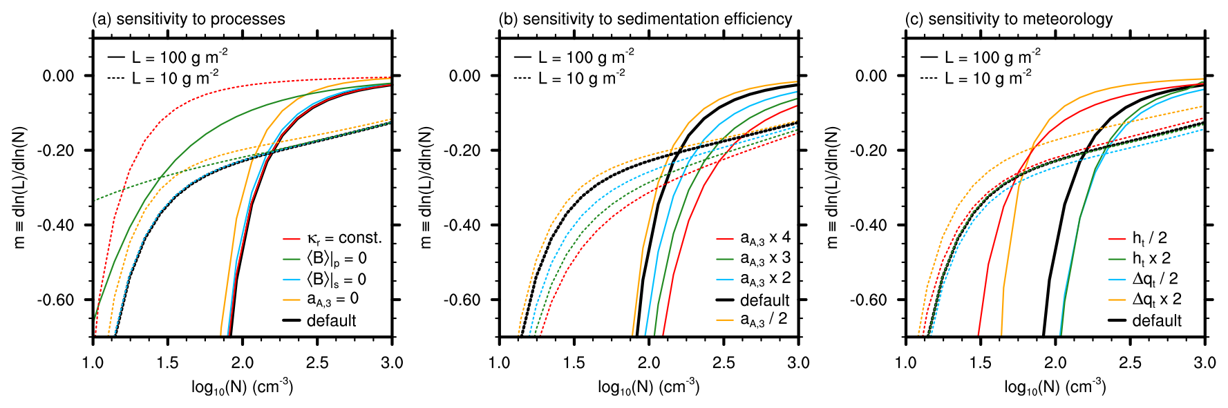
Figure 3 Panels (a)–(c) show m as a function of N for $L=\mathrm{10}\mathrm{g}{\mathrm{m}}^{-\mathrm{2}}$ (dashed lines) and 100 g m⁻² (continuous lines), with a thick black line indicating the default case. Colored lines highlight the sensitivity of m to (a) processes, (b) sedimentation efficiency, and (c) meteorology.

Figure 3a shows how m depends on the representation of various processes considered in the estimate of w_e. To remove the dependence of the emission of longwave radiation on N, a constant effective emissivity of ${\mathit{\kappa }}_{\mathrm{r}}=\mathrm{85}{\mathrm{m}}^{\mathrm{2}}{\mathrm{kg}}^{-\mathrm{1}}$ instead of the radius-dependent κ_r used above is applied (red lines). For $L=\mathrm{100}\mathrm{g}{\mathrm{m}}^{-\mathrm{2}}$, m is not substantially affected by this change, which is expected since the emission of longwave radiation is saturated. For $L=\mathrm{10}\mathrm{g}{\mathrm{m}}^{-\mathrm{2}}$, however, m weakens substantially from −0.23 to a negligible value of −0.03 at $N=\mathrm{100}{\mathrm{cm}}^{-\mathrm{3}}$ and vanishes completely for higher N. This indicates that the dependency of longwave radiation on N is the major driver for cloud water adjustments in weakly and non-precipitating clouds at low L. This picture reverses when the influence of precipitation on 〈B〉 is neglected by setting $\langle B\rangle {|}_{\mathrm{p}}=\mathrm{0}$ (green lines). For $N=\mathrm{100}{\mathrm{cm}}^{-\mathrm{3}}$, the absence of precipitation weakens m from −0.48 to −0.10 for $L=\mathrm{100}\mathrm{g}{\mathrm{m}}^{-\mathrm{2}}$, while it changes negligibly from −0.23 to −0.22 for $L=\mathrm{10}\mathrm{g}{\mathrm{m}}^{-\mathrm{2}}$. At $N=\mathrm{1000}{\mathrm{cm}}^{-\mathrm{3}}$, inhibiting precipitation does not change m for any L value. Thus, evaporating precipitation is the main driver for m for $N=\mathrm{100}{\mathrm{cm}}^{-\mathrm{3}}$ and high L, while it does not affect m at low L or high N.

We disregard the sedimentation–entrainment effect by setting a_A,3=0 in Eq. (28) (orange lines). For $L=\mathrm{100}\mathrm{g}{\mathrm{m}}^{-\mathrm{2}}$, the absence of sedimentation–entrainment weakens m from −0.48 to −0.32 at $N=\mathrm{100}{\mathrm{cm}}^{-\mathrm{3}}$, indicating a substantial but smaller impact than evaporating precipitation. For higher N and lower L, sedimentation becomes weaker, as does the influence of the sedimentation–entrainment feedback. However, the sedimentation–entrainment feedback is still responsible for the bulk of cloud water adjustments for $L=\mathrm{100}\mathrm{g}{\mathrm{m}}^{-\mathrm{2}}$ at $N=\mathrm{1000}{\mathrm{cm}}^{-\mathrm{3}}$, where its absence weakens m from −0.03 to −0.01. For $L=\mathrm{10}\mathrm{g}{\mathrm{m}}^{-\mathrm{2}}$, on the other hand, longwave radiation exceeds the impact of the sedimentation–entrainment feedback for all analyzed N values, with m weakening only from −0.23 to −0.20 at $N=\mathrm{100}{\mathrm{cm}}^{-\mathrm{3}}$ and −0.14 to −0.12 at $N=\mathrm{1000}{\mathrm{cm}}^{-\mathrm{3}}$ in the absence of the sedimentation–entrainment feedbacks. Note that neglecting sedimentation effects on 〈B〉 by setting $\langle B\rangle {|}_{\mathrm{s}}=\mathrm{0}$ (blue lines) affects m negligibly for all L values between N=100 and 1000 cm⁻³.

High-resolution modeling (direct numerical simulations) by de Lozar and Mellado (2017) indicates that the sedimentation–entrainment feedback can be about 3 times stronger than the estimate by Bretherton et al. (2007) based on large-eddy simulations. To analyze this, we varied a_A,3 from half to 4 times its default value (Fig. 3b). As expected, the effect of sedimentation–entrainment is proportional to a_A,3 and mostly visible for high L. For $L=\mathrm{100}\mathrm{g}{\mathrm{m}}^{-\mathrm{2}}$ and a_A,3×3 (continuous green line), we see a substantial strengthening of m from −0.48 to −0.80 at $N=\mathrm{100}{\mathrm{cm}}^{-\mathrm{3}}$ and −0.03 to −0.06 at $N=\mathrm{1000}{\mathrm{cm}}^{-\mathrm{3}}$, making the sedimentation–entrainment feedback comparable to the effect of evaporating precipitation at low N (Fig. 3a), while also allowing it to persist for higher N.

In Fig. 3c, we analyze the influence of two external (meteorological) parameters on m: boundary layer depth and free-tropospheric humidity, which are often considered to affect cloud water adjustments (e.g., Possner et al., 2020; Glassmeier et al., 2021). To address this, we vary h_t (red and green lines) and Δq_t (blue and orange lines) by halving or doubling their default values in Eq. (35), while keeping all other parameters the same. For $L=\mathrm{100}\mathrm{g}{\mathrm{m}}^{-\mathrm{2}}$, we find that m becomes more negative with h_t, in agreement with Possner et al. (2020) (red to black to green continuous lines). For $L=\mathrm{10}\mathrm{g}{\mathrm{m}}^{-\mathrm{2}}$, however, there is almost no effect of h_t (red to black to green dashed lines). This L dependence indicates that the main reason for the h_t dependence of m is the increased potential for evaporation of precipitation due to a deeper sub-cloud layer at higher h_t. Interestingly, we find that a drier free troposphere (Δq_t×2, orange lines) weakens cloud water adjustments, while a moister free troposphere ($\mathrm{\Delta }{q}_{\mathrm{t}}/\mathrm{2}$, blue lines) increases them, which is in contrast to Glassmeier et al. (2021) but in agreement with recent large-eddy simulations by Chun et al. (2023) and Chen et al. (2025). The reason for this behavior is twofold. First, increased moisture in the free troposphere reduces longwave radiative cooling at the cloud top, as considered in Eq. (18). Accordingly, the relative influence of L on longwave radiative cooling decreases, and a much stronger decrease in L is necessary to offset an increase in w_e to fulfill Eq. (35). At the same time, a moister free troposphere is more positively buoyant, which increases Δb. As above, a much stronger decrease in L is necessary to offset an increase in w_e in this situation.

4 Summary and conclusions

Cloud water adjustments strongly modify the ability of clouds to reflect solar shortwave radiation and hence their role in Earth's radiation budget (e.g., Stevens and Feingold, 2009). However, the magnitude and even the sign of cloud water adjustments are insufficiently understood (e.g., Boucher et al., 2013; Forster et al., 2021). This is especially true for weakly and non-precipitating stratocumulus, in which various processes tend to increase the mixing of the cloud with the free troposphere (entrainment) in response to an increase in aerosol and hence droplet concentration N, resulting in a decrease in the vertically integrated cloud water content L due to evaporation.

This study was built upon the assumption that an increase in entrainment rate w_e due to an increase in N is exactly offset by a commensurate decrease in L, resulting in the same w_e irrespective of N. This idea is based on large-eddy simulations presented in our companion paper (Chen et al., 2025) (see their Fig. 4a) and can be considered a corollary of the w_e–L feedback mechanism suggested by Zhu et al. (2005) (see their Fig. 7). This assumption, combined with a w_e parameterization developed for stratocumulus-topped boundary layers (Nicholls and Turton, 1986; Turton and Nicholls, 1987), enabled us to determine $m\equiv \mathrm{d}\ln \left(L\right)/\mathrm{d}\ln \left(N\right)$, the common metric to quantify cloud water adjustments, in an almost completely analytical way. Note that the m derived in this study is only valid for stratocumulus with negligible surface precipitation, and the effect of precipitation suppression on m (e.g., Albrecht, 1989) was not considered. Moreover, real clouds might not fully offset the increase in w_e due to an increase in N, with commensurate impacts on L and m. Thus, this study does not aim to provide a full quantitative understanding of cloud water adjustments but to untangle the effects of various processes comprising cloud water adjustments of weakly and non-precipitating stratocumulus.

We showed that three processes are mainly responsible for negative cloud water adjustments in weakly and non-precipitating stratocumulus: first, we showed that the full evaporation of precipitation below cloud base, commonly referred to as virga, is a major source for negative cloud water adjustments (Caldwell et al., 2005; Wood, 2007; Sandu et al., 2008; Uchida et al., 2010). Although virga affects only a limited range of the analyzed stratocumulus, it is able to stabilize boundary layer dynamics and hence to decrease w_e. Thus, an increase in N strengthens boundary layer dynamics and hence w_e, with commensurate negative impacts on L. Second, w_e decreases when sedimentation removes liquid water from the cloud top (Bretherton et al., 2007), which limits the necessary preconditioning of to-be-entrained air by the evaporation of cloud water (Yamaguchi and Randall, 2012). Reducing the sedimentation of liquid water by an increase in N, L decreases due to an increase in w_e. This so-called sedimentation–entrainment feedback is found to affect clouds with sufficiently high L but is exceeded by the aforementioned effect of virga at low N. However, the sedimentation–entrainment feedback becomes the primary source of negative cloud water adjustments at high N. Note that the sedimentation–entrainment feedback could be stronger according to modeling by de Lozar and Mellado (2017). Third, we showed that the droplet size dependence of longwave radiation causes negative cloud water adjustments, but only when longwave radiative cooling is not saturated, i.e., for clouds with $L<\mathrm{30}\mathrm{g}{\mathrm{m}}^{-\mathrm{2}}$ (e.g., Garrett et al., 2002; Petters et al., 2012).

Previously, it has been suggested to describe cloud water adjustments in weakly and non-precipitating stratocumulus by a constant m<0 (Gryspeerdt et al., 2019; Glassmeier et al., 2021). Our study showed, however, that these negative cloud water adjustments tend to be relatively strong at small N ($m=-\mathrm{0.48}$ at $N=\mathrm{100}{\mathrm{cm}}^{-\mathrm{3}}$) and weaken toward larger N ($m=-\mathrm{0.03}$ at $N=\mathrm{1000}{\mathrm{cm}}^{-\mathrm{3}}$) due to the cessation of precipitation and sedimentation effects. This weakening of m toward larger N is found to be slower for $L<\mathrm{30}\mathrm{g}{\mathrm{m}}^{-\mathrm{2}}$, where unsaturated longwave radiation has to be considered. A similar weakening of negative cloud water adjustments is shown in the large-eddy simulations of our companion paper (Chen et al., 2025) (see their Fig. 1b and d).

Moreover, our study showed that deeper boundary layers exhibit stronger negative cloud water adjustments, in agreement with Possner et al. (2020), which we explained by the increased potential for the full evaporation of precipitation below cloud base, i.e., a higher potential for virga. Further, we showed that increasing free-tropospheric humidity strengthens negative cloud water adjustments, in contrast to modeling by Glassmeier et al. (2021) but in agreement with Chun et al. (2023) and our companion paper (Chen et al., 2025). Because w_e weakens as the free-tropospheric humidities increases, stronger (relative) reductions in L were necessary to offset the increase in w_e following an increase in N.

Finally, we would like to speculate on the timescales associated with the negative cloud water adjustments laid out in this study. Our results suggest that these adjustments are required to accelerate boundary layer dynamics when the stabilizing effect of virga is suppressed by an increase in N. At higher N, however, negative cloud water adjustments are determined by the increasing supply of preconditioned free-tropospheric air (Yamaguchi and Randall, 2012; Bretherton et al., 2007). One might argue that the timescale associated with this process is shorter, as it does not require the acceleration of boundary layer dynamics (see Feingold et al., 2015). (The vertically averaged buoyancy flux 〈B〉 in Fig. 1d exhibits a much stronger gradient toward higher N at low N than at high N.) While our work cannot determine timescales associated with the changes in boundary layer dynamics, it does suggest that the timescale for cloud water adjustments should decrease toward higher N.

All in all, this study showed that even comparably simple models, such as the one used here, can be applied to increase our fundamental understanding of aerosol–cloud interactions. In fact, the simplicity of the applied model allowed us to directly link the cause and effect of cloud water adjustments, which can be difficult in more complex models such as global circulation or even large-eddy simulation models due to confounding factors (Mülmenstädt et al., 2024). That being said, the nuance provided by these models should not be disregarded as they help to quantify the effects that have been neglected here (e.g., interactive surface fluxes, changes in boundary layer depth, and the diurnal cycle of solar radiation). Thus, we advocate that the assessment of aerosol–cloud interactions should balance the use of complex and simple approaches by substantiating quantitative understanding with qualitative insight.