Quantifying biases in TROPESS AIRS, CrIS, and joint AIRS+OMI tropospheric ozone products using ozonesondes

Quantifying changes in global and regional tropospheric ozone is critical for understanding global atmospheric chemistry and its impact on air quality and climate. Satellites now provide multi-decadal records of daily global ozone profiles, but previous studies have found large disagreements in satellite-based ozone trends, including in trends from different products based on the same spectral radiances. In light of these disagreements, it is critical to quantify to what degree the observed trend is attributable to measurement error for each product by comparing satellite-retrieved ozone to long-term measurements from ozonesondes. NASA's TRopospheric Ozone and its Precursors from Earth System Sounding (TROPESS) project provides satellite retrievals of ozone from a suite of instruments, including Cross-track Infrared Sounder (CrIS), Atmospheric Infrared Sounder (AIRS), and multispectral combinations such as AIRS and Ozone Monitoring Instrument (OMI) (joint AIRS+OMI) using a common algorithm. We compare these products to ozonesondes and find that the evolution of global tropospheric ozone satellite–sonde biases for TROPESS CrIS (0.21 ± 3.6 % decade⁻¹, 2016–2021), AIRS (−0.41 ± 0.57 % decade⁻¹, 2002–2022), and joint AIRS+OMI (1.1 ± 1.0 % decade⁻¹, 2004–2022) are less than the magnitude of trends in global tropospheric ozone reported by the Tropospheric Ozone Assessment Report Phase 1 (TOAR-I). We further quantify the bias in regional trends, which tend to be higher but with a smaller number of sondes, which can impact the satellite–sonde bias and trend. Our work represents an important basis for the utility of using satellite data to quantify changes in atmospheric composition in future studies.

1 Introduction

Tropospheric ozone trends show large regional variations and can depend strongly on the type of measurement analyzed, coverage, frequency, and vertical sensitivity. The Tropospheric Ozone Assessment Report (TOAR) aims to provide the most complete assessment of tropospheric ozone available to the community by compiling a comprehensive database of ozone measurements and analyzing data from multiple sources holistically. The Sixth Assessment Report (AR6) produced by the Intergovernmental Panel on Climate Change (IPCC) reports that the global tropospheric ozone burden (TOB) is increasing, but regional trends detected by three ensembles of satellite data ranged in magnitude from 2 % decade⁻¹ to 14 % decade⁻¹ (Gulev et al., 2021). The ensembles in Gulev et al. (2021) combine satellite instruments that retrieve ozone in the ultraviolet (UV), visible, and/or near-infrared (NIR) ranges but do not include instruments that retrieve ozone in the thermal infrared (TIR) range. Some TIR instruments have reported negative tropospheric ozone trends in various regions (e.g., Pope et al., 2024; Dufour et al., 2025). The satellite assessment in phase 1 of TOAR (TOAR-I; Gaudel et al., 2018) speculated that causes of inter-satellite disagreement include differences in each instrument's vertical sensitivity to the atmospheric profile of ozone, spatial sampling across the globe, and measurement period.

Ongoing work in TOAR phase 2 (TOAR-II) aims to investigate the causes of measurement-dependent differences in ozone trends and find consensus across techniques to determine the true TOB trend. There are a range of reported tropospheric ozone trends from work published in the past decade (Table 1) that tend to agree that tropospheric ozone is increasing globally and in most specific latitude bands but to varying degrees and with varying levels of certainty. These recent studies discuss two major reasons for discrepancies between satellite ozone products. The first is that the vertical sensitivity of each instrument impacts the amount of measured ozone in each level of the atmosphere (Gaudel et al., 2018). Some instruments and retrievals can distinguish influences from the upper versus lower troposphere (Pope et al., 2023, 2024; Froidevaux et al., 2025), which can lead to different assessments of how tropospheric ozone is changing if these changes are not uniform in altitude. Second, the satellite product quality can drift over time, producing an artificial trend caused by error in the instrument calibration or retrieval (Gaudel et al., 2018). Gaudel et al. (2024) demonstrated a method to correct the tropospheric ozone trend for the time-dependent bias to produce a tropospheric ozone trend. This was accomplished by quantifying the bias between satellite data and a reference method, e.g., ozonesonde data. The magnitude of the bias was used to scale the satellite data to determine trends in tropospheric ozone with the retrieval bias (approximately) removed.

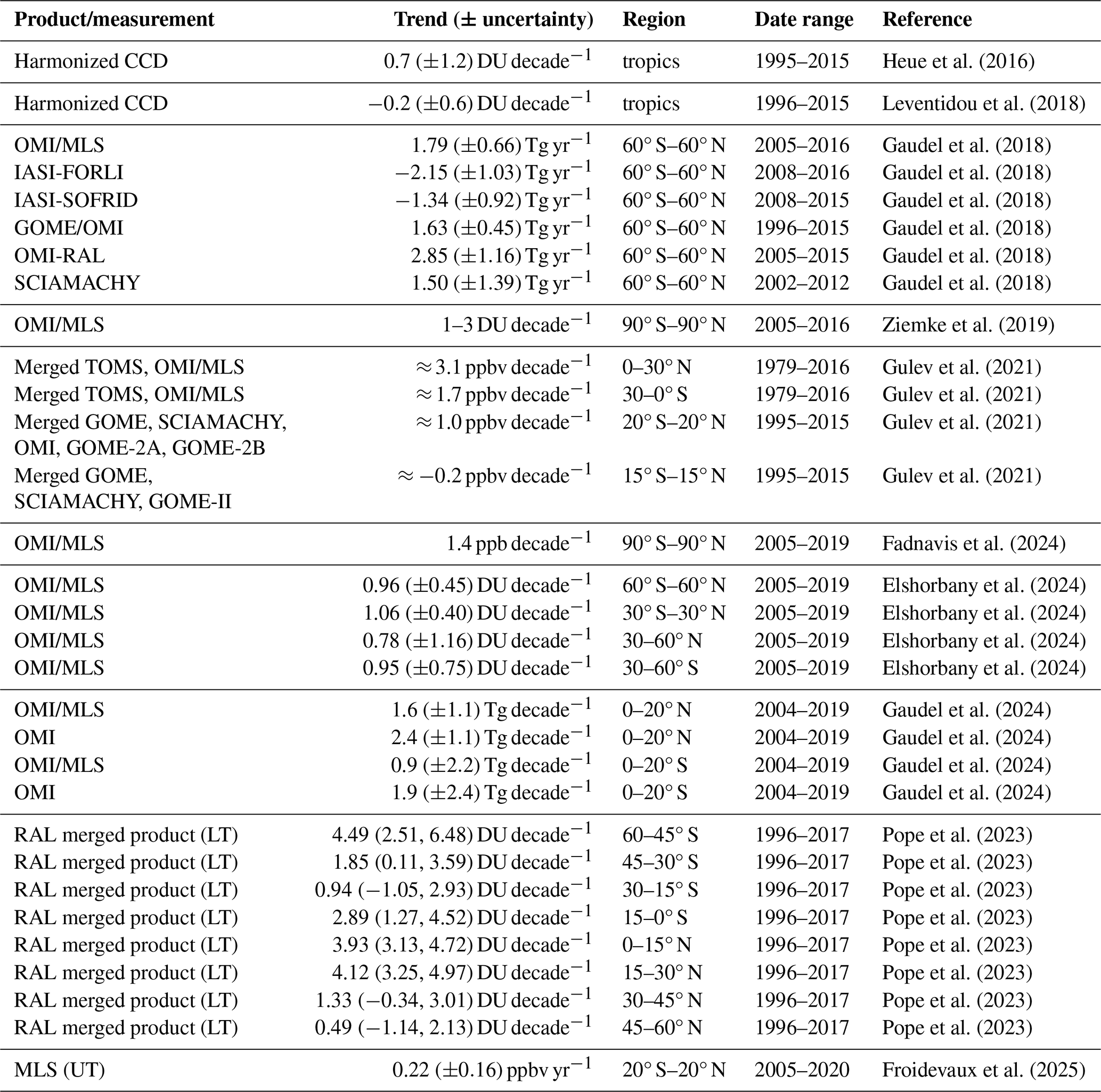
Heue et al. (2016)Leventidou et al. (2018)Gaudel et al. (2018)Gaudel et al. (2018)Gaudel et al. (2018)Gaudel et al. (2018)Gaudel et al. (2018)Gaudel et al. (2018)Ziemke et al. (2019)Gulev et al. (2021)Gulev et al. (2021)Gulev et al. (2021)Gulev et al. (2021)Fadnavis et al. (2024)Elshorbany et al. (2024)Elshorbany et al. (2024)Elshorbany et al. (2024)Elshorbany et al. (2024)Gaudel et al. (2024)Gaudel et al. (2024)Gaudel et al. (2024)Gaudel et al. (2024)Pope et al. (2023)Pope et al. (2023)Pope et al. (2023)Pope et al. (2023)Pope et al. (2023)Pope et al. (2023)Pope et al. (2023)Pope et al. (2023)Froidevaux et al. (2025)

Table 1 Tropospheric ozone burden (TOB) trends from satellite products reported in the literature (LT represents lower troposphere; UT represents upper troposphere). For the Rutherford Appleton Laboratory (RAL) merged product, uncertainty is displayed at the 95 % confidence interval.

Ozonesondes provide a long-term record of detailed vertical ozone profiles and thus are an important tool for quantifying the vertical distribution of ozone and therefore have been useful in validating satellite retrievals of ozone. Ozonesondes are mounted on atmospheric balloons that are routinely launched from over 40 sites worldwide (WMO/GAW, 2024). These sites are distributed unevenly, with many sites located in North America and Europe and fewer sites in the Southern Hemisphere. There are multiple types of ozonesondes, including electrochemical concentration cell (ECC; Komhyr, 1969; Komhyr and Harris, 1971; Tarasick et al., 2021; WMO, 2021) and Brewer–Mast (BM; Brewer et al., 1997; Steinbrecht et al., 1998) sondes. Most ozonesonde launch sites use ECC sondes, which typically have an uncertainty of 10 %–20 % (WMO, 2021). The Harmonization and Evaluation of Ground-based Instruments for Free Tropospheric Ozone Measurements (HEGIFTOM) working group of TOAR-II was developed with the goal of improving the accuracy and precision of ozone measurements by removing inhomogeneities between ozonesondes caused by differences in equipment, operating procedures, or data processing. The working group utilized a harmonization technique to address this need and has reduced ozonesonde measurement uncertainty to 5 % (5 %–10 % in the tropics) (WMO, 2021). The state-of-the-art method produces sonde data with high accuracy, precision, and long-term reliability, making them a good tool for validating other measurement methods.

We introduce here three satellite tropospheric ozone products that were not part of the TOAR-1 assessment and use the HEGIFTOM ozonesonde measurements to assess their suitability for quantifying trends in TOB. The TRopospheric Ozone and its Precursors from Earth System Sounding (TROPESS) project (NASA, 2024) provides retrievals of ozone and other trace gases from a suite of satellite instruments, including the Cross-track Infrared Sounder (CrIS), Atmospheric Infrared Sounder (AIRS), and a joint retrieval product using AIRS and the Ozone Monitoring Instrument (OMI) (joint AIRS+OMI). These satellite products provide long-term records of ozone using a consistent retrieval algorithm that produces ozone profiles that use the same a priori profiles and are calculated on the same vertical grid and with the same method of uncertainty estimation, making them more readily comparable. This study aims to validate the accuracy of TROPESS satellite retrievals of tropospheric ozone and their stability with time against ozonesonde measurements. Section 2 introduces the satellite and ozonesonde datasets and describes the analysis tools used to compare them. Section 3 presents comparisons between satellite and ozonesonde profiles and columns, long-term trends in the satellite–sonde bias, and temporal and geographic variations in these quantities.

2 Data and methods

2.1 TROPESS ozone retrievals

All TROPESS Level 2 data are produced using the MUSES – MUlti-SpEctra, MUlti-SpEcies, MUlti-SEnsors – algorithm (Fu et al., 2013, 2016, 2018), following the optimal estimation methods employed for the EOS Tropospheric Emission Spectrometer (TES) (Beer, 2006; Bowman et al., 2006). This approach estimates vertical profiles, uncertainty estimates, and observation operators, which are critical for chemical data assimilation and inverse modeling (Jones et al., 2003; Parrington et al., 2009; Miyazaki et al., 2017, 2020b). Three TROPESS products are considered in this study: CrIS, AIRS, and the joint AIRS+OMI retrieval, and they have been used in previous studies to monitor changes in global tropospheric ozone (Miyazaki et al., 2021) and understand the processes controlling air pollution (Miyazaki et al., 2019).

CrIS, AIRS, and OMI data have been used to generate Level 2 products by other teams and retrieval algorithms. For example, the Community Long-term Infrared Microwave Combined Atmospheric Product System (CLIMPCAPS), NOAA Unique Combined Atmospheric Processing System (NUCAPS), and Near Real Time (NRT) Standard Physical Retrieval (AIRS2RET_NRT_7.0) produce Level 2 CrIS and AIRS products that are retrieved from Level 2 cloud-cleared radiances on a 45 km field of regard (Smith and Barnet, 2020; Barnet et al., 2021; AIRS, 2019). The single field-of-view (SFOV) sounder atmospheric product (SiFSAP) retrieval algorithm produces Level 2 CrIS, AIRS, and IASI products from Level 1B radiances (Wu et al., 2023). The TROPESS project generates Level 2 products using Level 1B radiances processed by the MUSES algorithm. The three TROPESS products are described further in Sect. 2.1.1–2.1.3.

The global, monthly average tropospheric ozone columns are computed from the ozone profiles retrieved by MUSES and are shown in Fig. 1 for the three products. The average tropospheric column – integrated over the ozone profile from the surface to the thermal tropopause (see Sect. 2.3) – falls between 30 and 40 Dobson units (DU), with the ozone seasonal cycle clearly visible. Each satellite product provides data for different time periods and with different average magnitudes, which will be discussed in Sect. 3. The trends in the TROPESS ozone products are not monotonic, largely due to the decrease in ozone during the COVID-19 pandemic (Miyazaki et al., 2021). Therefore, they require careful consideration when being compared to the trends in bias shown in the current study. Such analysis will be the topic of a follow-on manuscript.

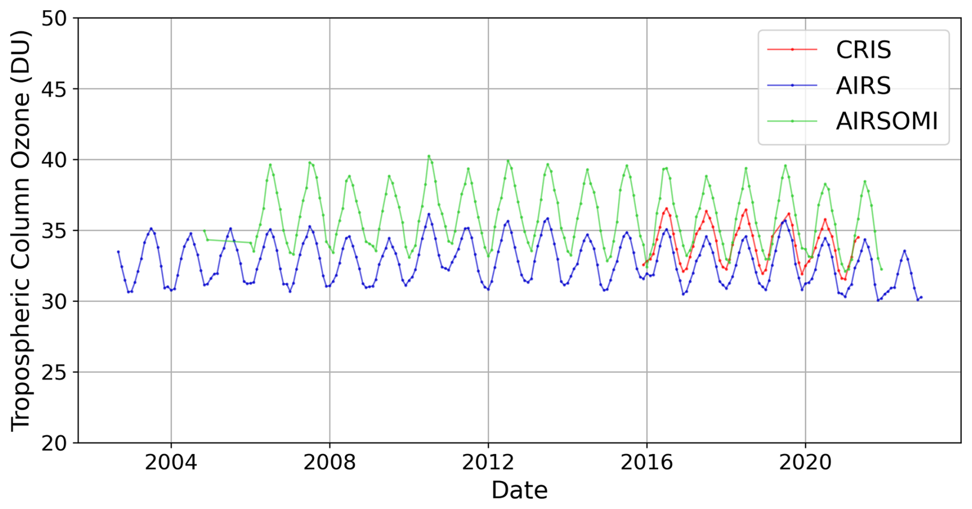
Figure 1 Global (67° S–85° N) monthly average tropospheric ozone columns for the TROPESS CrIS (red), AIRS (blue), and joint AIRS+OMI (green) products.

2.1.1 CrIS

CrIS is on the Suomi National Polar-orbiting Partnership (SNPP) satellite, which was launched on 28 October 2011 and has a 13:30 LT (local time) ascending node (Han et al., 2013). CrIS instruments are also flying on the Joint Polar Satellite Series platforms (JPSS-1 and JPSS-2). However, for this study we focus only on SNPP-CrIS data so that we use one consistent record (with, for example, consistent calibration, spatial sampling, and temporal sampling) for our trend analysis. CrIS has high spectral resolution, high signal-to-noise ratio, and a low calibration uncertainty (Han et al., 2013; Strow et al., 2013; Tobin et al., 2013; Wang et al., 2013). CrIS measures infrared (IR) radiances in three bands: 650–1090 cm⁻¹ (long-wave IR, LWIR), 1210–1750 cm⁻¹ (mid-wave IR, MWIR), and 2155–2550 cm⁻¹ (short-wave IR, SWIR) (Han et al., 2013). TROPESS ozone retrievals from CrIS specifically use four windows in the LWIR and six windows in the MWIR (Malina et al., 2024). TROPESS CrIS Level 2 products are retrieved from the L1B radiances on individual 15 km fields of view. The CrIS data record begins in 2012, but the radiance data that were initially retrieved only have nominal spectral resolution (NSR): 0.625 cm⁻¹ in the LWIR band, 1.25 cm⁻¹ in the MWIR band, and 2.5 cm⁻¹ in the SWIR band (Han, 2015). In November 2015, the data record grew to include the full spectral resolution (FSR) of 0.625 cm⁻¹ in all three bands. The TROPESS project uses the NASA L1B FSR radiance data (Revercomb and Strow, 2018), so our record begins in November 2015 (Han, 2015). In late March 2019, there was an anomaly in the MWIR band, resulting in a gap in data from April through July 2019. The instrument was restored to full functionality, and there is good consistency between the early and later 2019 data (Iturbide-Sanchez et al., 2022). In July 2021, there was a failure in the LWIR bands that required the instrument to change to a different set of electronics (NOAA, 2021), and the data acquired after this date were no longer included in the long-term record by NASA. Therefore, the ozone record used in this study runs from December 2015 through May 2021. Given the large variability in tropospheric ozone and the small magnitude of its trends, the TROPESS CrIS record is too short to detect ozone trends with good statistical significance. Nonetheless, we consider the time dependence of the CrIS–sonde bias using the same analysis process as with the other two TROPESS products, because we focus here on whether there are any changes in the retrieval quality with time as well as on the consistency of the TROPESS products. In particular, TROPESS CrIS and AIRS both utilize IR radiances, and their comparison is of particular interest. We discuss the impact of the relatively short CrIS time range with respect to bias detection in Sect. 3.2. Our analysis is a necessary step if the TROPESS CrIS product is to be used as part of a longer-term merged tropospheric ozone record in the future.

2.1.2 AIRS

AIRS is a thermal infrared (TIR) grating spectrometer aboard the Aqua satellite, launched on 4 May 2002 (Aumann et al., 2003; Susskind et al., 2003, 2014). Aqua is part of the A-train, a constellation of satellites that orbit together (Stephens et al., 2002). AIRS has a 13 km footprint at nadir and measures in the 650–2675 cm⁻¹ wavelength range (Aumann et al., 2003; Susskind et al., 2003), with ozone retrieved from channels around 1042 cm⁻¹ (Wei et al., 2010). Similarly to CrIS, TROPESS retrieves ozone from AIRS from L1B radiances (AIRS, 2007) using 10 distinct wavelength windows in the IR (Fu et al., 2018). TROPESS AIRS Level 2 products are retrieved from the L1B radiances on individual 15 km fields of view.

2.1.3 Joint AIRS+OMI retrieval

OMI, unlike CrIS and AIRS, measures ozone-absorbing radiances in the UV range (Levelt et al., 2006, 2018; Liu et al., 2010a, b; Huang et al., 2017). OMI flies on the Aura satellite, a member of the A-train, so it collects data at nearly the same local time as AIRS. Retrievals of ozone from OMI use wavelengths between 270 and 365 nm with a ground pixel size of 12 × 24 km (Levelt et al., 2006). OMI experienced a “row anomaly” beginning in 2007. In 2009, the anomaly spread, and many pixels became unusable; since 2010, ∼ 40 %–50 % of OMI pixels must be discarded. In addition to the lower data volume, there have been small changes to OMI radiances (1 %–2 %) and irradiances (3 %–8 %), but overall the number of good pixels remains stable (Schenkeveld et al., 2017).

Fu et al. (2018) combined AIRS and OMI radiances in a joint retrieval to produce the joint AIRS+OMI product. This multispectral retrieval, implemented in the MUSES algorithm, uses information in the AIRS TIR bands and the OMI UV bands to produce vertical ozone profiles. The joint AIRS+OMI product has greater vertical sensitivity than the AIRS or OMI retrievals alone, with degrees of freedom of signal (DOFS) in the troposphere ranging from 0.2 to 1.6, typically falling above 1 (Fu et al., 2018). Because the DOFS exceed 1, it is possible to resolve ozone subcolumns in the troposphere, i.e., upper and lower tropospheric ozone.

2.2 Ozonesonde data

ECC sondes are mounted alongside radiosondes to provide the partial pressure of ozone, total atmospheric pressure, and atmospheric temperature (Tarasick et al., 2019). These quantities can be used to calculate the volume mixing ratio (VMR) of ozone throughout the profile until the balloon pops, typically before reaching 5 hPa. Ozonesonde data are provided by the HEGIFTOM working group of TOAR-II (Van Malderen et al., 2025). The sonde launch sites providing data for this study are shown in Fig. 2a.

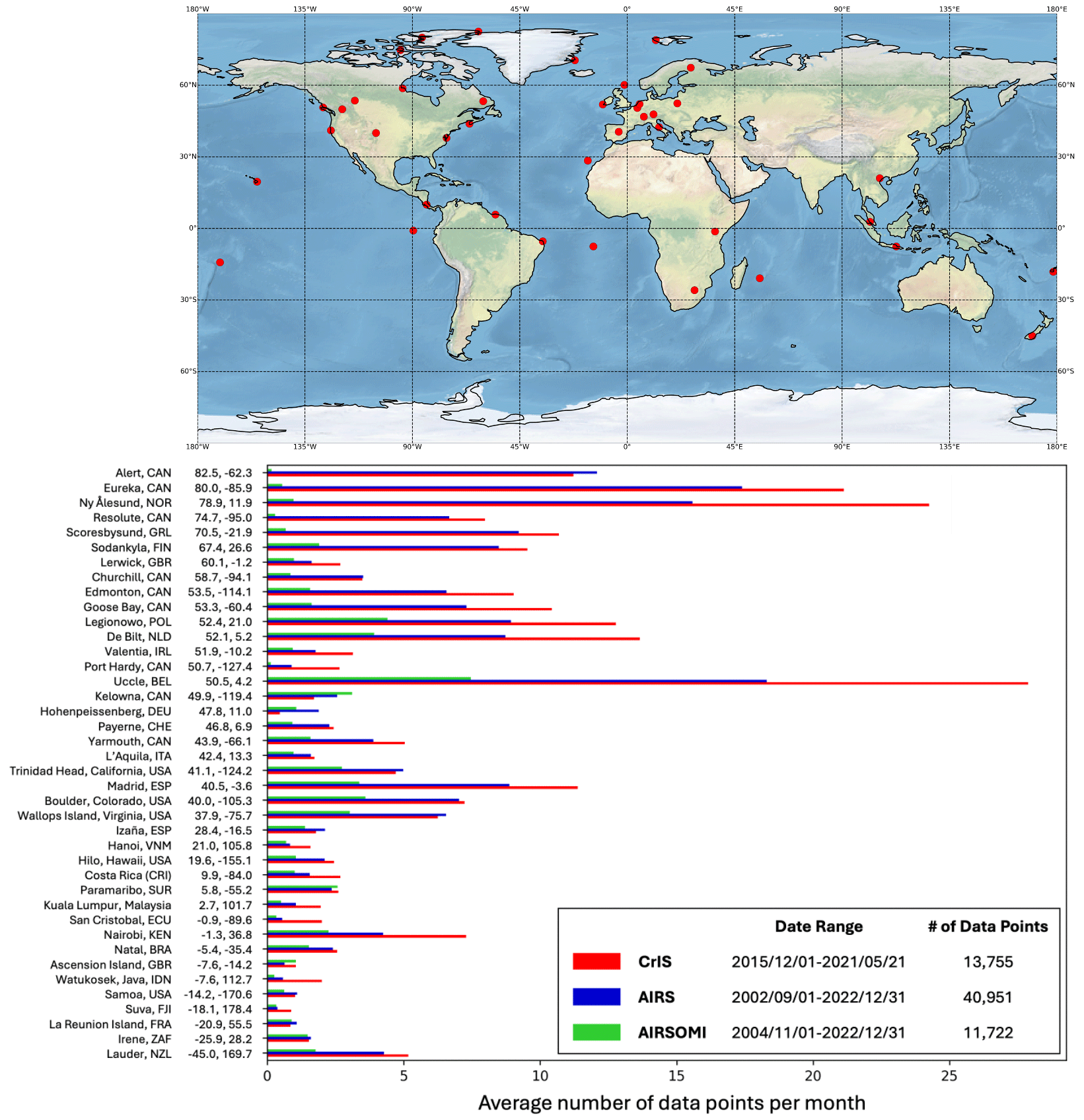
Figure 2 (a) Ozonesonde launch sites providing harmonized data in this study. (b) Monthly average number of matched satellite–sonde data points at each sonde launch site for each satellite product. Sites are ordered by decreasing latitude. The figure legend provides the date range of each satellite product and the total number of matched satellite–sonde data points over the date range at all sites.

2.2.1 Coincidence criteria

Sonde and satellite profiles are compared if the sonde is launched within 300 km and 9 h of the satellite measurement. These criteria may result in multiple satellite profiles being matched with a single sonde profile. These spatial and temporal thresholds were chosen to compare measurements from similar air masses while being large enough to capture sufficient data for a statistically meaningful comparison and to maintain consistency with previous studies (Nassar et al., 2008; Verstraeten et al., 2013). However, the choice of coincidence criteria can impact the satellite–sonde bias. Nassar et al. (2008) showed that wide spatial and temporal coincidence criteria can lead to comparisons between satellite and sonde profiles that measured air columns with high atmospheric and ozone variability. When they tightened the spatial and temporal coincidence criteria, the value of the bias did not change in a statistically meaningful way, but the standard deviation increased. This implies that comparing profiles with different atmospheric profiles adds random error but does not introduce a positive or negative bias (Nassar et al., 2008). So, we maintain these coincidence criteria – 300 km and 9 h – in our study.

2.2.2 Application of the satellite operator

To directly compare satellite and sonde profiles, the satellite retrieval operator must be applied to the sonde data to account for satellite sensitivity and vertical resolution (Jones et al., 2003; Worden et al., 2007; Verstraeten et al., 2013; Malina et al., 2024). This operation is performed on the sonde data to estimate the ozone profile that the satellite would have measured had it observed the same air mass as the sonde, with no systematic or random errors other than those attributable to the smoothing of the profile due to the vertical sensitivity of the satellite. The satellite operator includes the averaging kernel, and an a priori constraint vector together; examples of these quantities are shown in Fig. 3. The following steps describe the application of the satellite operator to a sonde profile.

1. Sonde measurements are provided on fine vertical grids with variable maximum altitudes. All TROPESS profiles are provided on 67 fixed levels reaching a minimum pressure of approximately 1 hPa. If the minimum pressure (i.e., maximum altitude) of the sonde profile is greater than the minimum pressure of the satellite profile for a matched pair of a satellite profile and sonde profile, then the ozone concentrations from the satellite prior are appended to the sonde profile concentrations, scaling the prior so that the concatenated concentration profile is continuous. This step ensures that the satellite and sonde profiles reach the same minimum pressure.

2. The sonde profile is interpolated to the same 67 pressure levels as the satellite profile.

3. The satellite operator is applied according to Eq. (1). x_sonde is the new sonde profile, which can be directly compared to the satellite profile; x_a is the a priori profile; A is the averaging kernel; and x_{sonde,measured} is the sonde profile produced following steps 1 and 2. Example profiles and the averaging kernel from a single CrIS sounding are presented in Fig. 3, and representative averaging kernels for each instrument are given in Fig. S4 in the Supplement.

$$\begin{array}{}\text{(1)}& {\mathit{x}}_{\mathrm{sonde}}={\mathit{x}}_{\mathrm{a}}+\mathit{A}({\mathit{x}}_{\mathrm{sonde},\mathrm{measured}}-{\mathit{x}}_{\mathrm{a}})\end{array}$$

After the satellite operator is applied to the sonde profile, the profiles must be quality controlled. Poor quality in the resampled sonde profiles may result from either poor quality in the original sonde profiles (x_{sonde,measured}) or poor behavior when the satellite operator is applied to x_{sonde,measured}. The HEGIFTOM group did not quality control (QC) the sonde data, so we tested multiple methods of QC, explained in Sect. S1 in the Supplement. To evaluate each QC method, we considered the impact on the mean, median, standard deviation, and trend of the tropospheric ozone column satellite–sonde bias, as well as the percentage of profiles removed. See Sect. S1 for a detailed description of the methods that were tested and the metrics used to evaluate the QC methods.

Our selected quality control method considers the stratosphere and troposphere separately. In the stratosphere, profiles are compared to a climatology from the Aura Microwave Limb Sounder (MLS), an instrument launched in 2004 aboard the Aura satellite that provides stratospheric profiles of multiple atmospheric gases (Livesey et al., 2022; Waters et al., 2006; Werner et al., 2023) and has been validated using ozonesonde and lidar measurements (Jiang et al., 2007). The accuracy of the MLS-retrieved ozone in the upper troposphere is within 5 % compared to ozonesonde data, except in the tropics where the 2σ uncertainty can reach 10 % (Livesey et al., 2022). The Level 3 MLS dataset includes the mean ozone profile and standard deviation at each level, binned into latitude bands spaced every 10° (Fig. S5). We assume that any ozone mixing ratio that falls outside of the mean MLS profile ±5 standard deviations in a specific latitude band is physically impossible, so if a sonde or satellite VMR falls outside of these limits at any level, that profile is removed from the analysis. MLS only measures ozone in the upper troposphere and above, so the ozonesonde concentrations within the troposphere are compared to the distribution of the TROPESS satellite ozone profiles. For each satellite–sonde set (e.g., AIRS + sondes), each sonde profile is compared to the mean ±5 standard deviations of the distribution of satellite profiles. If any concentrations in the sonde profile fall outside of this range, the profile is removed from the analysis. This process is performed in the troposphere for each set of matched satellite–sonde profiles. Using this method of QC, the percentage of profiles removed from CrIS, AIRS, and joint AIRS+OMI comparisons are 4.5 %, 3.5 %, and 5.7 %, respectively.

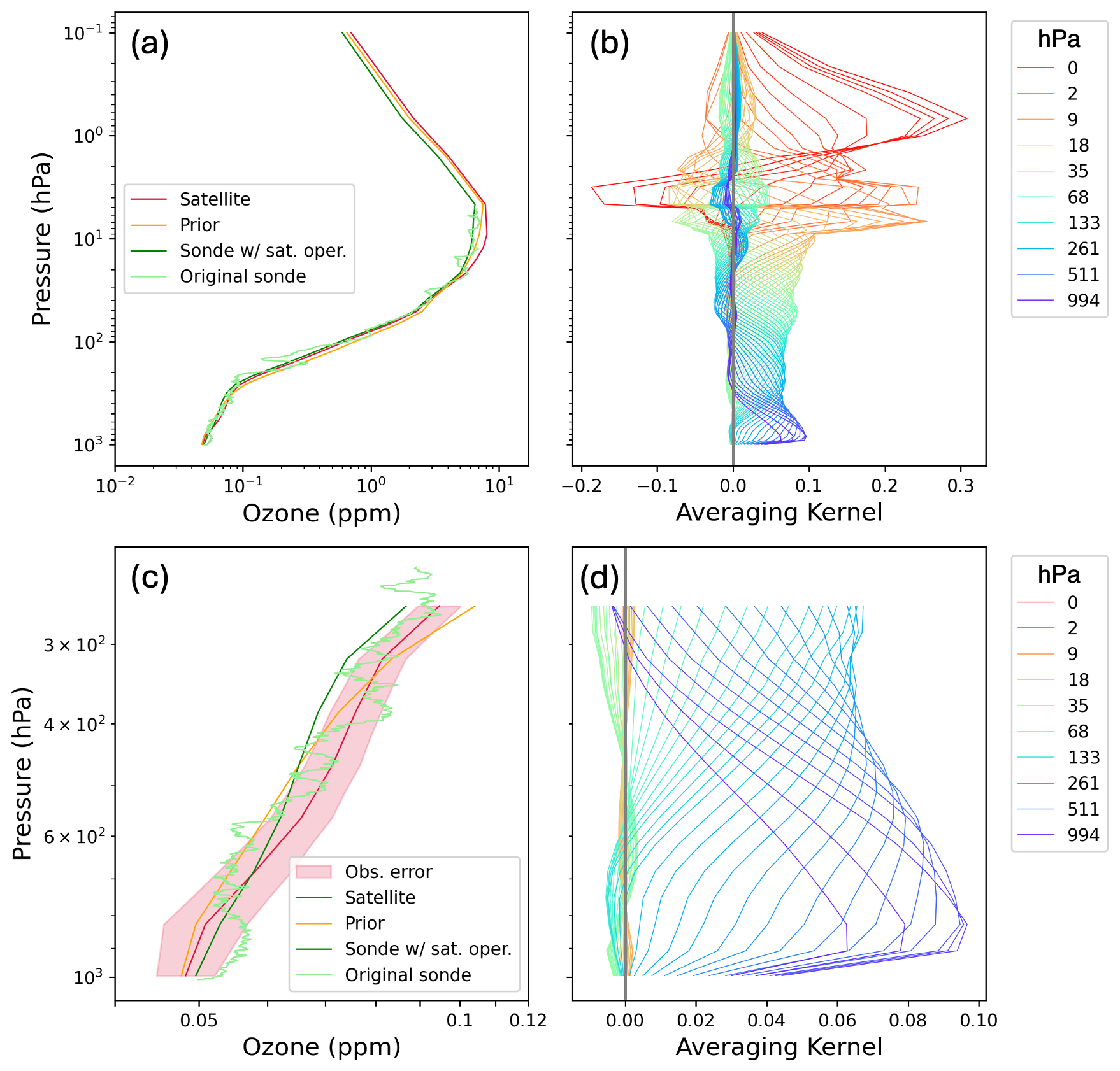
Figure 3 Example ozone profiles and averaging kernels from a comparison of a CrIS retrieval to an ozonesonde. (a) Ozone profile retrieved from the satellite (red), prior profile used in the CrIS retrieval (orange), profile measured by the ozonesonde (light green), and profile produced when the satellite operator is applied to the ozonesonde measurement (dark green). (b) Averaging kernel corresponding to the same retrieval in (a). (c, d) Same as (a) and (b) with the vertical extent cropped to focus on the troposphere. The red shading in (c) indicates the observation error of the satellite profile.

The number of matched and filtered data points for each satellite product at each sonde launch site is given in Fig. 2b. The differences in the number of matched data points between satellite products is due to the differences in sampling, satellite data throughput, and time period of data collection (see Sect. 2.1.1–2.1.3).

2.3 Column calculations

The MUSES algorithm method is used to calculate total ozone columns and ozone subcolumns. The total ozone column is calculated by integrating the ozone from the surface to the top of the atmosphere – the highest-altitude point in the TROPESS products, around 0.1 hPa. Calculating a subcolumn requires the definition of the maximum and minimum pressure levels for the column, as well as temperature and water vapor profiles to account for factors such as the Bernoulli equation and deviation from the ideal gas law. Temperature and water vapor profiles are provided by the TROPESS project (NASA, 2024).

Tropospheric columns are integrated from the surface to the thermal tropopause, as defined by the World Meteorological Organization (WMO) (WMO, 1957). The thermal tropopause is obtained from version 5 of the NASA Global Modeling and Assimilation Office (GMAO) Goddard Earth Observing System (GEOS-5) model Forward Processing for Instrument Teams (FP-IT) (Molod et al., 2012; GMAO, 2024; Lucchesi, 2015) and is specific to the date, time, and location of each data point. TROPESS defines the lower tropospheric column to extend from the surface to 500 hPa and the upper tropospheric column to extend from 500 hPa to the tropopause.

2.4 Correlation and trend analysis

The percent bias is calculated for every profile, column, and subcolumn according to Eq. (2).

$$\begin{array}{}\text{(2)}& \text{Percent bias}={\displaystyle \frac{C_{\mathrm{satellite}}-C_{\mathrm{sonde}}}{C_{\mathrm{sonde}}}}\cdot \mathrm{100}\mathit{\%}\end{array}$$

The calculation of trends follows guidance presented by the TOAR-II statistics focus working group (Chang et al., 2023). In brief, we use quantile regression (QR) to report trends at the 50th percentile. In comparison to other trend detection methods, QR is preferred due to its robustness to small sample sizes and outliers and its ability to account for non-normal error distributions and autocorrelation. The TOAR-II guidance also provides a method for moving block bootstrapping that we use to calculate the uncertainty of trends and assign a p value to communicate the likelihood that a trend exists. Moving block bootstrapping calculates the standard error of the trend over multiple subsamples (blocks) along a time series, and it is used to accurately quantify the trend uncertainty while taking autocorrelation and heteroskedasticity into account (Chang et al., 2023). Satellite–sonde correlation coefficients (r²) are calculated using simple linear regression. To explore the geographic variability of ozone levels and data quality, results are grouped by latitude bands that are spaced every 30°.

3 Results

3.1 Satellite–sonde comparisons

The satellite and sonde profiles matched for each satellite product (Fig. S6) were used to derive profiles of percent difference for the three TROPESS products globally and within each latitude band (Fig. 4). The global mean percent bias profiles all fall within 20 % bias, with the vertical distribution of bias varying by product. Each satellite instrument has a different vertical sensitivity, as indicated by the averaging kernels (Figs. 3 and S4), which results in differences in the ozone vertical profile. However, because each satellite operator has been applied to each sonde profile, the biases primarily reflect differences in the air mass sampled within the coincidence criteria along with systematic and random errors in the satellite retrievals. The magnitude and vertical distribution of bias varies across latitude bands, but there is more variability across instruments than across latitude for each instrument. Figure 4 illustrates the high volume of data in the northern midlatitudes and high latitudes compared to the tropics and Southern Hemisphere, due to the lack of ozonesonde data in the Southern Hemisphere.

The TOB is represented by tropospheric column ozone (Fig. 1), so we calculate the percent bias between matched satellite- and sonde-measured columns. A time series of monthly averaged percent bias between matched satellite and sonde tropospheric ozone columns between 30 and 60° N is shown in Fig. 5a. The 50th percentile (i.e., median) of all of the points is given in the legend for each satellite product, and it is displayed in the left-hand bar chart (Fig. 5b) for all latitude bands. All three satellite products tend to overestimate tropospheric ozone columns in all latitude bands, with AIRS having the lowest positive bias. Joint AIRS+OMI tends to have the largest median bias, but the CrIS median bias can be of a comparable magnitude to joint AIRS+OMI (e.g., Fig. 5b, 60–90° N). The median percent bias at each sonde site is given in Fig. S7a. The median bias is positive at most sites, but there are some negative median bias values. There can be large differences in the bias of the three products at some sites, and even sites within the same latitude band do not necessarily show consistent biases. The same analysis as shown in Fig. 5 but using absolute bias (in Dobson units) is shown in Fig. S8.

To better understand the differences in satellite bias between products, the 50th percentile percent bias for each latitude band in both the lower troposphere (LT) and upper troposphere (UT) is given in Fig. 6. The largest overpredictions are in the UT, where satellite sensitivity tends to be greater (Fig. S4). The distribution of bias in the UT across latitude bands is consistent with the overall tropospheric column bias. In the LT, AIRS and CrIS biases fluctuate around 0 DU. AIRS and CrIS have lower sensitivities in the LT, so there is little true information in this altitude range, and the lack of bias primarily reflects the use of the same prior profile in both the satellite measurements and the sonde measurements with the satellite operator applied. Joint AIRS+OMI has greater sensitivity in the LT than the other two products, and it also tends to have the largest magnitude bias; it is negative at northern high latitudes but positive in all other regions.

The TROPESS products' tropospheric ozone biases are similar to the bias between other satellite products and ozonesondes. The mean tropospheric column ozone bias between the Tropospheric Emission Spectrometer (TES) and ozonesondes was shown to range from 7 % to 15 % (Verstraeten et al., 2013) or approximately 2.9 DU (Osterman et al., 2008), with the UT displaying a wider range of bias than the LT (Nassar et al., 2008; Verstraeten et al., 2013). Our results show a decreased tropospheric column bias compared to TES (Fig. 5b), with a consistent distribution of bias between the UT and LT compared to TES. Whereas the three satellite products studied in this work display positive mean biases in most locations, other satellites display negative biases in some latitude bands. Boynard et al. (2018) showed that the IASI (Infrared Atmospheric Sounding Interferometer)/Metop-A (IASI-A) and IASI/Metop-B (IASI-B) tropospheric ozone products had mean biases compared to sondes ranging 4 % to 5 % in high latitudes, −4 % to −5 % in midlatitudes, and −16 % to −19 % in the tropics. The OMI/MLS product presented by Ziemke et al. (2019) reported a mean bias of −2 DU for the tropospheric column ozone compared to global ozonesondes between 60° N and 60° S. Miles et al. (2015) showed a mean bias of approximately 10 % (2 DU) in the Northern Hemisphere and from −15 % to −20 % (−1 to −3 DU) in the Southern Hemisphere for the Global Ozone Monitoring Experiment 2 (GOME-2) RAL (Rutherford Appleton Laboratory) ozone retrieval. The median bias of the GOME-2 RAL product compared to sondes in the lower troposphere is approximately −1 DU (−6 %) globally, −0.5 DU (−3 %) in the NH, and ∼0 DU in the SH (Pope et al., 2023). Pope et al. (2023) also quantified the bias of the RAL GOME-1, OMI, and SCIAMACHY lower tropospheric ozone columns compared to ozonesondes. The median bias of RAL GOME-1 is −5 DU (−26 %) globally, −5 DU (−26 %) in the NH, and −1 DU (−7 %) in the SH; the median bias of RAL OMI is −4 DU (−19 %) globally, −5.5 DU (−24 %) in the NH, and −3.5 DU (−19 %) in the SH; and the median bias of RAL SCIAMACHY is 2 DU (12 %) globally, 2 DU (11 %) in the NH, and 3.5 DU (28 %) in the SH. While the sign of the mean biases can vary between satellite products, the absolute values are of approximately the same order of magnitude, suggesting that the TROPESS products are of a similar quality as existing satellite products. Gaudel et al. (2018) calculated a mean TOB of 301 Tg with a range of 281–318 Tg across five satellite products. The 37 Tg range is equivalent to approximately ±6 % of the average TOB. The differences in satellite–sonde bias across satellite products, ranging from −3 to 3 DU as shown in our results and the previous studies summarized here, likely accounts for at least some of the difference in measured TOB presented in Gaudel et al. (2018).

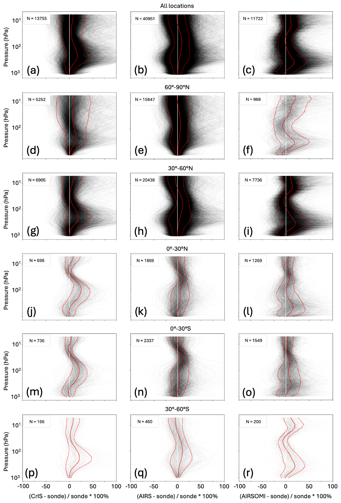
Figure 4 Percent bias between each matched satellite and sonde profile for CrIS (left), AIRS (center), and joint AIRS+OMI (right). The top row includes data at all sites, and subsequent rows contain data in each 30° latitude band. The solid red lines represent the mean difference profile, and the dashed red lines represent 1 standard deviation away from the mean. The number of profiles in each latitude band is indicated by the density of the individual black lines. The solid white lines are at 0 %.

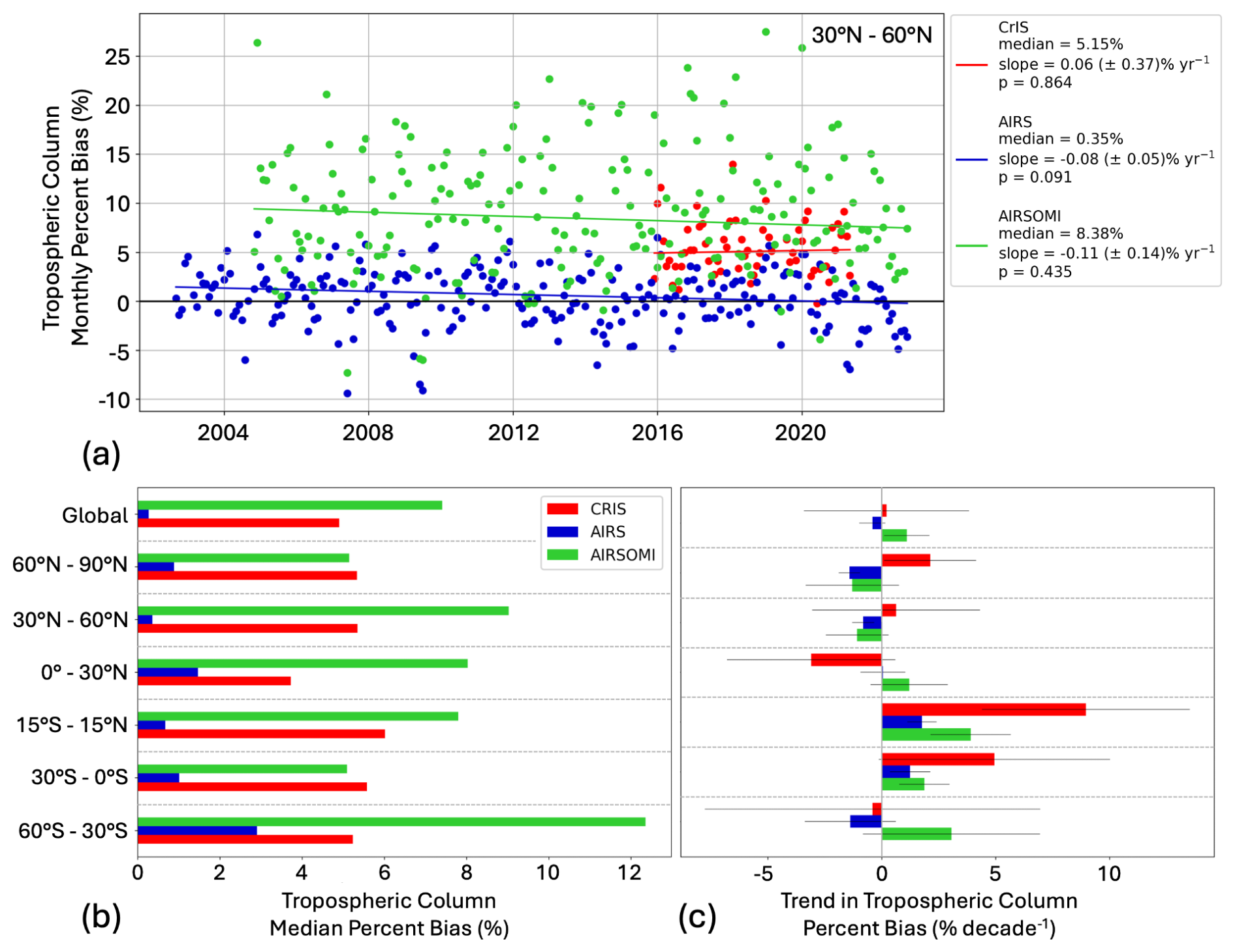
Figure 5 (a) Monthly averaged tropospheric column percent bias for all sites between 30 and 60° N. The slope, standard error of the slope, and p value of the slope are reported for the 50th percentile. The medians and slopes reported in the bottom row are derived from time series such as this. (b) The median tropospheric column percent bias in each latitude band. (c) The trend in tropospheric column percent bias in each latitude band. There are no sonde sites between 60 and 90° S.

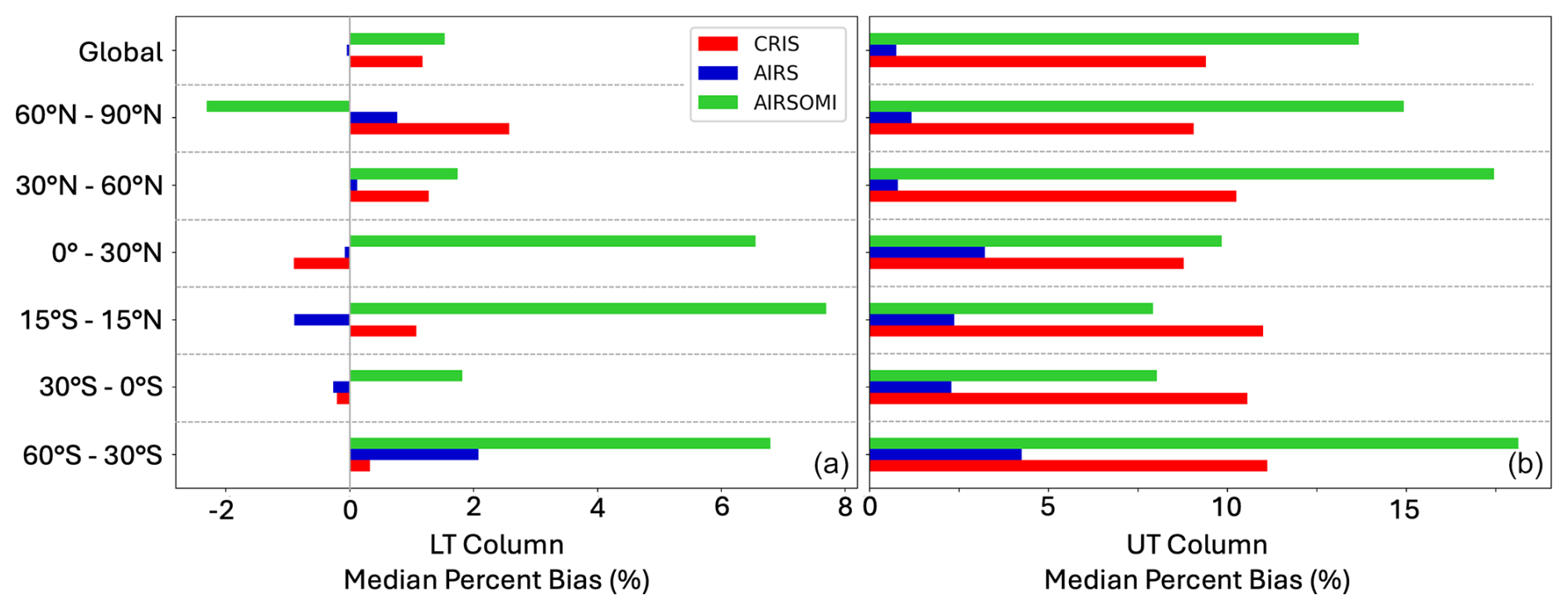
Figure 6 The median LT (a) and UT (b) column percent bias averaged over sites in each latitude band. There are no sonde sites between 60 and 90° S.

3.2 Trends in satellite–sonde bias

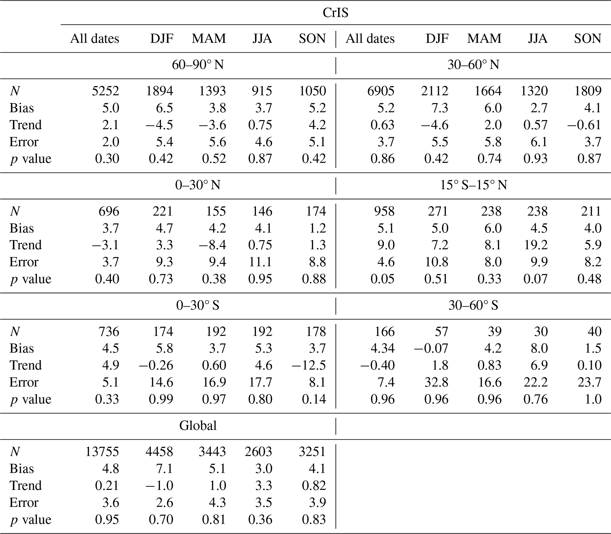
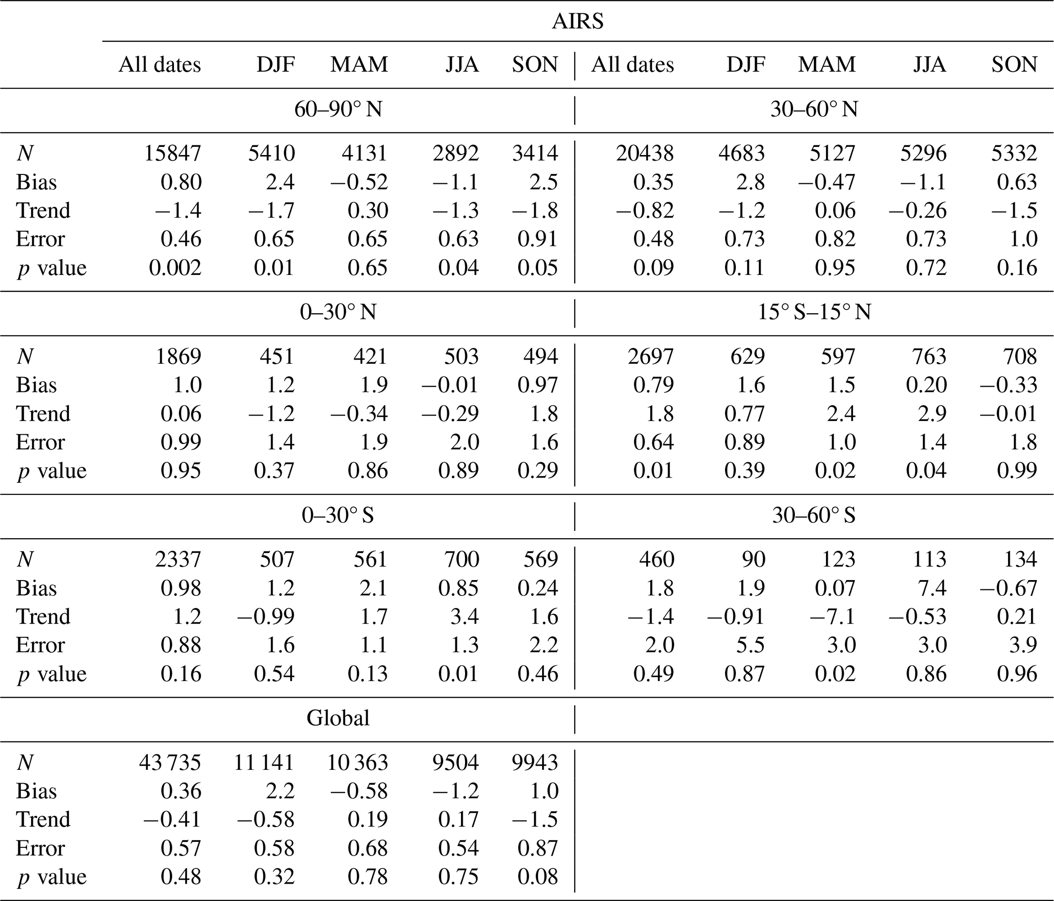
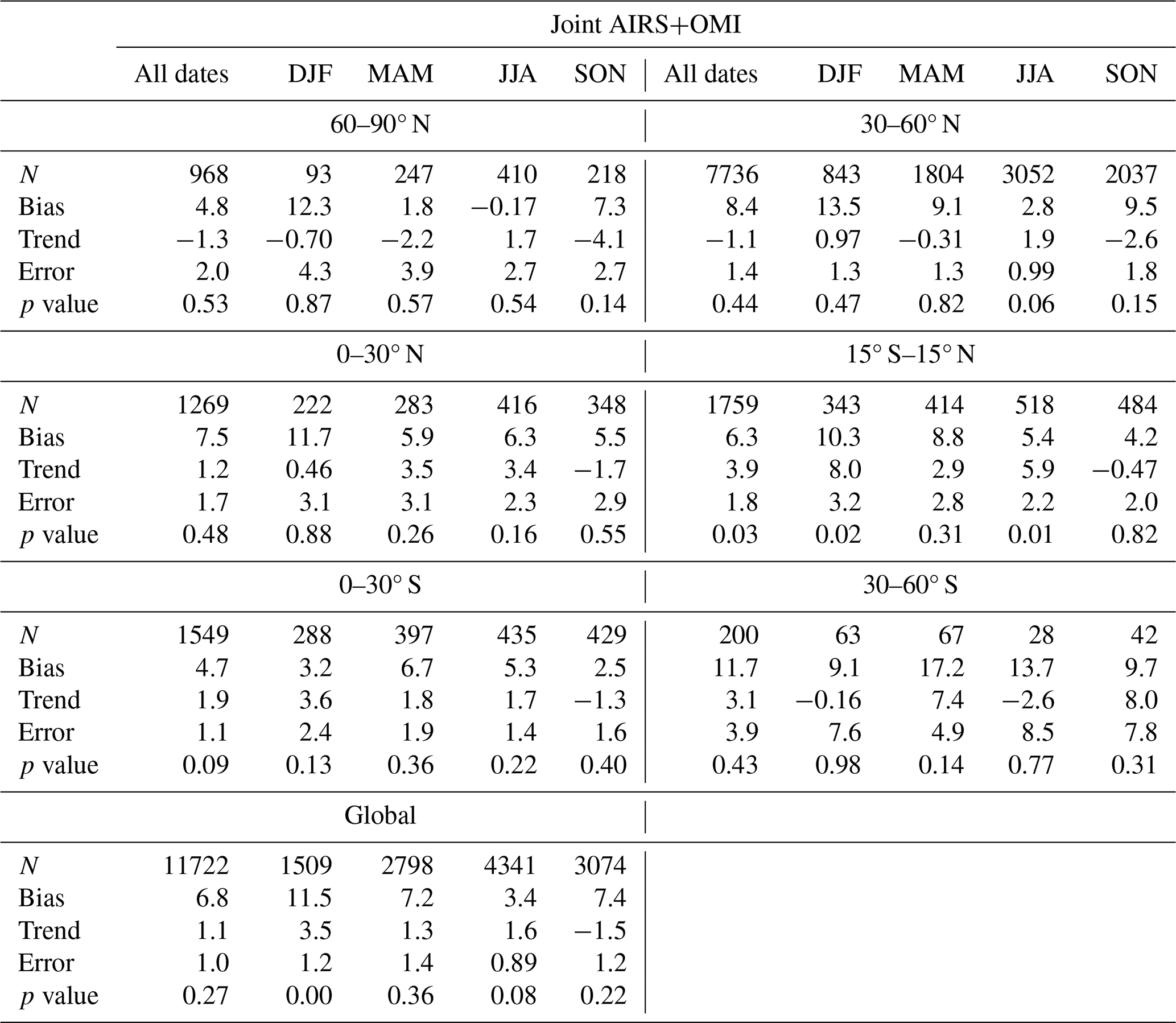
The time series of tropospheric ozone column biases (such as that shown in Fig. 5a) is used to calculate the trend in satellite–sonde bias and its uncertainties. The trends for each product are shown in the legend of Fig. 5a and for all latitude bands in Fig. 5c. Figure S8 displays the trends in concentration units (DU decade⁻¹), and Fig. S7b displays the trends for each sonde launch site. The trend in satellite–sonde bias is within ±2 % decade⁻¹ for all products globally. Gulev et al. (2021) reported regional TOB trends ranging from 2 to 14 % decade⁻¹ (1–6 ppbv decade⁻¹). Globally, the trends in bias fall below the low end of that range (2 % decade⁻¹) by a factor of 1–10.

When reported in each latitude band, the magnitude of the bias trend tends to be larger, and the sign can vary. In most regions, the standard error in the trend (represented by the black lines in Fig. 5c) is larger than the trend itself, and the p values are large (Table S4). This suggests that the trends have very low certainty and cannot be distinguished from a trend of zero; thus, they should not influence the TOB trend detection. This is not true in the tropics, however, where there are relatively larger trends and smaller errors. This feature is investigated further in Sect. 3.3. A previous study comparing IASI-A and IASI-B to ozonesondes found an average drift of −8.6 (±3.4) % decade⁻¹ (−2.81 (±1.26) DU decade⁻¹) in the Northern Hemisphere (Boynard et al., 2018). The TROPESS products all have drift values less than that value, excluding CrIS in the tropics. Because most of the sonde data are collected in northern midlatitudes, the global average satellite–sonde bias is most strongly influenced by the data in those latitude bands. The bias trends reported in the 60–30° S band were calculated using data at only one ozonesonde site: Lauder, Aotearoa / New Zealand (Fig. 2). While these data may not be representative of the entire latitude band, we choose to include the results because the Lauder site has a relatively high data volume and is an important source of data in the Southern Hemisphere (Fig. 2b). Additionally, the profiles of satellite–sonde bias at the Lauder site (Fig. 4p–r) display similar features as the profiles in other latitude bands, suggesting that the Lauder site provides meaningful data. The ability of one site to represent trends throughout a region is discussed further in Sect. 4.

To further investigate the spatial distribution of biases in satellite retrievals, we quantify the correlation between the satellite–sonde biases at different sonde launch sites. If the monthly time series of percent bias at different sites are uncorrelated, then the satellite products are providing geographically independent data. As an example, the bias time series at one site (e.g., Uccle, Belgium) was compared to the bias time series at a second site (e.g., Valentia, Ireland), and the r² between the time series data was calculated. This analysis was performed between all pairs of sites, and the r² values are given in Fig. S9. High r² values indicate a relationship between the bias in different locations, while a low r² value indicates no relationship. The r² values are consistently low between sites, even sites that are in similar regions such as Europe (De Bilt, Valentia, Uccle, Hohenpeissenberg, Payerne, L'Aquila, and Madrid) or western North America (Trinidad Head, Port Hardy, Kelowna, and Edmonton). This suggests that satellite–sonde bias is random and not systematic by location. While the sonde sites do not represent the entire globe and are not evenly distributed, this preliminary analysis suggests that the satellite performance is not strongly location dependent.

The satellite products cover different time periods, with CrIS providing data for the shortest time period. To compare the products during only their overlapping time periods, the AIRS and joint AIRS+OMI data were cropped to the same time period as CrIS, and the median percent bias and the trend in the percent bias were calculated in the same manner as Fig. 5 (see Fig. S10). The change in the median percent bias between the two time periods was minor at almost all sites, but the magnitude of the trend in the bias increased at many sites. At the same time, the standard errors of the trends tend to be larger than the trends themselves, and many of the p values are large (i.e., over 0.33, Fig. S10), meaning that the trends in bias during this time period are uncertain and may not be differentiable from zero (Chang et al., 2023). The large errors highlight the difficulty of trying to determine a trend over a short time period, particularly for a trace gas with large interannual variability like tropospheric ozone. While one may be tempted to infer that these 2015–2021 bias trends indicate the current performance of the AIRS and joint AIRS+OMI satellite products, the uncertainty of the trends suggests that 5 years is not a sufficient period for trend detection. The results also imply that the relatively large trends in bias seen in CrIS as compared to the other two instruments are primarily driven by the short length of the record rather than by any instability or deficiency in the CrIS product.

3.3 Seasonal dependence of biases

The seasonal dependence of tropospheric, UT, and LT column satellite–sonde comparisons is shown in Fig. 7. Seasonal dependencies arise in CrIS and AIRS, because they are both TIR instruments; thus, their sensitivity to ozone depends on the thermal structure of the atmosphere, particularly the thermal contrast between the surface and the lowest layer of the atmosphere. The sensitivity of OMI likewise varies with season, as it depends strongly on solar insolation. As expected, AIRS and CrIS have similar seasonal patterns, with the smallest standard deviations in SON and the largest standard deviations in DJF. The seasonal spread of AIRS and CrIS is relatively small in the LT, likely because of their low sensitivity there, with most of the seasonal differences occurring in the UT. High standard deviations in the UT in DJF are caused by high ozone values (Fig. S11) occurring in the northern high latitudes (Fig. S12). Figures S11–S12 are presented for AIRS, but similar ozone distributions are seen in the CrIS dataset. The joint AIRS+OMI product has low data volume near the poles and does not properly capture the long tail of the ozone distribution in northern high latitudes. Because the high ozone values are seen in both the satellite records and the sondes, they are likely to be real. Previous work used the Modern-Era Retrospective analysis for Research and Applications Version 2 (MERRA-2) global reanalysis model to show the prevalence of multiple tropopauses at northern high latitudes (Manney et al., 2017). Multiple tropopauses often form when upper tropospheric jets impinge on the high-altitude tropopause in the tropics, causing high-altitude tropospheric air to bend poleward into regions with lower-altitude tropopauses (Manney et al., 2014). Multiple tropopauses allow for enhanced mixing between the troposphere and stratosphere, allowing for high stratospheric ozone concentrations to intrude into the troposphere and raise ozone concentrations. Manney et al. (2017) also found a high frequency of multiple tropopauses in high southern latitudes in JJA, but we do not observe high ozone values in JJA in the TROPESS datasets due to the lack of coincident satellite and sonde measurements below 60° S.

Figure 7 also demonstrates that joint AIRS+OMI has the lowest correlation with sonde measurements in all vertical regimes, with the largest difference between joint AIRS+OMI and the other two satellite products in the LT. Joint AIRS+OMI has the highest sensitivity in the LT compared to AIRS and CrIS (see Fig. S4) because it includes UV radiances from OMI, which are sensitive to the entire ozone column, including the surface (Fu et al., 2018). While it is clear that there is a systematic bias in the LT TROPESS joint AIRS+OMI retrievals, the relative lack of bias in AIRS and CrIS likely arises because their retrievals provide little information in the LT due to low sensitivity. Since the satellite operator is applied to the ozonesonde measurements, this lack of sensitivity results in both the retrieved satellite and the sonde profiles largely reverting to the prior values.

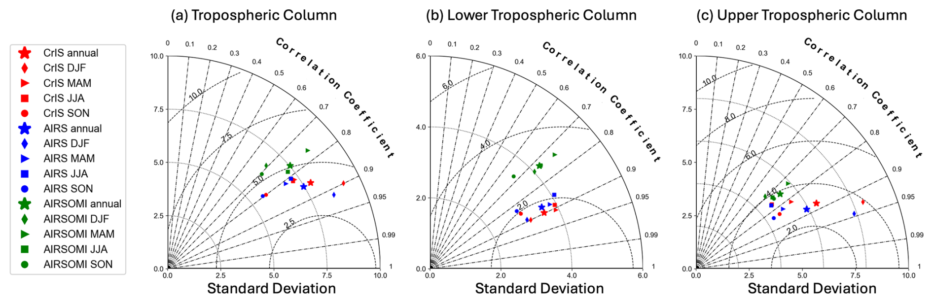
Figure 7 Taylor diagram representing global statistics of CrIS (red), AIRS (blue), and joint AIRS+OMI (green) tropospheric column comparisons with sondes. The radial distance from the origin represents standard deviation, azimuthal angle represents the correlation coefficient (r), and the dashed arcs centered on the x axis represent the root-mean-square error (RMSE). Markers represent datasets in each season (DJF: December–January–February; MAM: March–April–May; JJA: June–July–August; SON: September–October–November) and annually.

The satellite–sonde percent bias also varies across season (Tables 2, 3, 4). In the Northern Hemisphere, the bias is largest for all three products in DJF and smallest in JJA. This seasonal pattern is also reflected in the global values since most of the data fall in the Northern Hemisphere. In the Southern Hemisphere, the change in bias across seasons is less consistent, but this may be due to the lack of data in the Southern Hemisphere compared to the Northern Hemisphere. In all seasons, the CrIS and joint AIRS+OMI biases remain positive (except 30–60° S CrIS in DJF), whereas the AIRS bias is negative in the spring (MAM) and summer (JJA) in the Northern Hemisphere and spring (SON) in the Southern Hemisphere.

Seasonality is also seen in the trend in satellite–sonde bias and can explain why the trend in tropical percent bias is larger than that in other regions (Tables 2, 3, 4). There is little consistency in the seasonality of the bias trend across products, but it is noteworthy that the magnitudes of the seasonal bias trends are substantially larger for CrIS than the annual average trend in most regions. However, we caution against over-interpreting these results given the relatively short duration of the CrIS product. In many regions, the bias trend fluctuates between positive and negative values across seasons, resulting in a small annual average value for each product. But in the tropics (15° S–15° N), the bias trend is almost always positive, leading to the large trend in annual bias, particularly for CrIS (Fig. 5c). The satellite sensitivity to ozone tends to be largest in the tropics due to a combination of good thermal contrast, warm atmospheric temperatures, high insolation, and large ozone abundances. The variability in these parameters is also lowest in the tropics, so the sensitivity is more likely to be consistent across seasons. The seasonal dependence of the biases and how they vary across region and for each satellite product are important to consider when quantifying a trend in only one season or month. For example, some studies quantify the tropospheric ozone trend in summer only, since summer typically has the highest ozone values and worst air pollution. The impact of time-dependent satellite bias can be different in the summer season than for the annual average, so the bias in each time frame should be considered explicitly.

Table 2 Comparisons between CrIS and sonde tropospheric ozone columns: sample size (N), bias (%), trend (% decade⁻¹), error (standard error in the trend), and p value on the trend. Data are separated by region and season.

Table 3 Same as Table 2 but for AIRS.

Table 4 Same as Table 2 but for joint AIRS+OMI.

4 Discussion

The focus of this study was to comprehensively compare TROPESS tropospheric ozone products to ozonesonde data by quantifying satellite–sonde biases and their evolution with time. Nonetheless, we wish to emphasize that analyses must consider the time range used for trend detection, as a short time period may not provide enough information to detect trends with high precision. The CrIS dataset used here runs from late 2015 to mid-2021, and the uncertainties associated with the CrIS–sonde bias trends are high (Fig. 5 and Table S4), except in the tropics. Additionally, when the AIRS and joint AIRS+OMI datasets were cropped to the same time period as the CrIS record, the uncertainties in their bias trends were very large as well. The ability to quantify a drift with high precision depends on both the magnitude of the drift and its variability, with longer records required for smaller drifts and/or larger variability. It is critical that statistical methods such as block bootstrapping, which preserves the correlation between consecutive data points and therefore more accurately captures the variance of a time series than other methods, are used to assess statistical significance and to determine whether a given record is long enough to detect a trend.

A substantial portion of the effort underlying this analysis was directed at establishing QC methods for the ozonesonde data (Sect. 2.2.2 and the Supplement), and we wish to emphasize that this process can impact the outcome of validation (i.e., bias estimation) studies. While the ozonesonde data have low measurement uncertainty and have historically been used to represent true ozone values, some of the sonde data have poor quality or do not interact with the satellite operator in a physically realistic manner. In some cases, the ozonesonde concentrations are realistic in the stratosphere and not the troposphere, but the application of the satellite operator convolves the stratosphere and troposphere, making those profiles unusable. Typically, studies that utilize sonde data develop their own QC methods, especially when working with satellite operators from a variety of products. As shown in Sect. S1, the QC methods and subset of sonde data used can impact the quantification of satellite–sonde bias. So studies that use different QC methods may not be comparing their datasets to the same information.

Section S1 suggests important topics for users of sonde data to consider when comparing to satellite ozone products. First, sonde users should investigate the impact that QC methods have on their results. This is true for ozone trend studies and studies that quantify instrument bias using sonde data as the ground truth dataset. As illustrated in Sect. S1, the trend in satellite–sonde bias varied by an order of magnitude and sign, ranging from −0.24 % decade⁻¹ to 0.21 % decade⁻¹ (Table S2), depending on the QC method selected. The median bias and trend in bias stabilized when certain methods were employed (Tables S2, S3), suggesting that some methods provide more realistic and stable metrics than other methods. In addition to considering the stability of the bias, users should also consider the vertical profile of the bias, as different methods resulted in more or less physically realistic profiles at different levels (Fig. S2). Second, applying QC methods to the original sonde data may not be sufficient to completely QC the data when working with satellite operators, since the application of the satellite operator can introduce physically unrealistic behavior. On the other hand, studies focusing solely on the sonde data will need to apply QC methods to only the raw sonde data. Because observational operators vary by instrument and in both space and time, we cannot state that our optimal QC method is tailored for use with other datasets. Third, QC methods can use historical or modeled data (e.g., from satellites, ground-based systems, and global models) to provide physically realistic concentration limits. In this study, the MLS climatology provided a physical basis for the screening of unrealistic profiles in the stratosphere. Future work could investigate the curation of a long-term ozone climatology in the troposphere for use in QC screening. In summary, we recommend that future studies utilizing sonde data consider the impact of QC methods and how the chosen subset of sonde data compares to existing studies.

Another important consideration is whether the sonde sites are truly representative of global ozone and can be used to accurately quantify global satellite–sonde bias. The ozonesonde sites are mostly grouped in the northern mid-to-high latitudes (Figs. 2 and 4), with little coverage in the Southern Hemisphere and most continents apart from Europe and North America. There is only one sonde site providing harmonized data between 60 and 30° S (Lauder, Aotearoa / New Zealand), and there is no harmonized sonde data available below 60° S. In this study, we used harmonized ozonesonde data provided by the HEGIFTOM group as part of the TOAR-II project (Van Malderen et al., 2025), which did not include data at all sonde sites at the time of production. For example, some data in East Asia have not yet been harmonized, and this could limit our ability to evaluate satellite ozone performance over this region. Chang et al. (2024) showed that the sampling of hourly ozone measurements at the Mauna Loa Observatory could drastically impact the accuracy of long-term trend detection. This work also showed that small-scale meteorological variability affects the trends. These results were given at one site but demonstrate the impact of localized phenomena on trend detection from in situ observations, suggesting that individual sites may not be representative of regional trends if their temporal sampling or meteorology are inconsistent. Future work will focus on assessing the degree to which the satellite–sonde intercomparisons shown here are representative of broader changes in bias using a tropospheric chemistry reanalysis (Miyazaki et al., 2020a, b).

This study suggests important considerations for the TOAR community when performing validation or trend analyses that compare multiple satellite products. In addition to the factors presented above (i.e., time range, sonde QC methods, and geographic representativeness), the sensitivity of the instruments, the a priori information, and other factors in the retrieval algorithms can impact trend detection. The TROPESS products used in this study were retrieved using a consistent algorithm that used the same a priori information, tropopause definitions, and vertical grids for all products. In an ideal scenario, all satellite products used in intercomparison studies would also use these consistent variables. Importantly, they would also all be compared to ozonesonde or other in situ data using the same filtering criteria rather than comparing to a variable ground truth dataset. While this would require significant effort to accomplish the large number of available satellite products, these steps would allow for the most accurate comparison of satellite measurement error and quantification of tropospheric ozone.

5 Conclusions

This study compares long-term tropospheric ozone records from three satellite products and ozonesondes. The CrIS, AIRS, and joint AIRS+OMI products are those developed by the TROPESS project, which uses a common retrieval algorithm and consistent a priori information to provide ozone profiles with quantified uncertainties. A major goal of the TOAR-II project is to quantify long-term trends in tropospheric ozone, which requires understanding to what degree the observed trend is attributable to non-physical properties such as instrument measurement drift. The TROPESS products were compared to global ozonesonde data, and the magnitude of the trends in satellite–sonde bias for the three products (CrIS: 0.21 ± 3.6 % decade⁻¹, AIRS: −0.41 ± 0.57 % decade⁻¹, and joint AIRS+OMI: 1.1 ± 1.0 % decade⁻¹) are approximately 1 order of magnitude less than the reported range in tropospheric ozone trends (−7.1 % decade⁻¹ to 9.5 % decade⁻¹). This work suggests that the three TROPESS products can be used to accurately detect global tropospheric ozone trends. Future work to quantify trends in specific regions or seasons, however, should consider the impact that more localized satellite measurement drift has on trend detection. While the measurement drift could not be quantified with high precision in many regions or seasons (Fig. 5 and Tables 2–4), the tropics displayed unique behavior with consistently positive and non-zero drift in all instruments.