Tracing elevated abundance of CH₂Cl₂ in the subarctic upper troposphere to the Asian Summer Monsoon

The Asian Summer Monsoon (ASM) is a seasonal weather pattern characterized by heavy rains and winds, mainly affecting South and Southeast Asia during the summer months. The deep convection within the ASM is an important transport process for pollutants from the planetary boundary layer up to the tropopause region. This study uses in situ observations of CH₂Cl₂ from the PHILEAS (Probing High Latitude Export of Air from the Asian Summer Monsoon) aircraft campaign in late summer 2023 to examine the transport pathways and timescales for polluted air from the ASM to the extratropical upper troposphere and lower stratosphere (UTLS). CH₂Cl₂ mixing ratios of up to 300 ppt (≈ 500 % of the Northern Hemisphere background) were measured in the upper troposphere in the subarctic region. The three largest observed pollution events were analyzed with the help of the Lagrangian particle dispersion model FLEXPART, both in terms of their origin and their potential entry into the lower stratosphere. The results show that the East Asian Summer Monsoon (EASM) is the key pathway for transporting uncontrolled short-lived chlorinated substances (Cl-VSLSs) into the tropopause region, which contributes to an increase in tropospheric background levels with the potential to enter the lower stratosphere. The transport analysis of elevated mixing ratios shown here suggests that transport to the upper troposphere in the subarctic region did not occur through transport into the Asian Summer Monsoon Anticyclone (ASMA) with subsequent eddy-shedding events but rather by large convective transport contributions from the EASM. The projected entry into the lower stratosphere in the following days amounts to a few percent, indicating that the direct influence of these particular events on the lower stratosphere is probably minor.

1 Introduction

Short-lived chlorinated substances (Cl-VSLSs) have shown an increasing abundance in the atmosphere in recent years. These trace gases have local lifetimes of less than half a year and are not controlled by the Montreal Protocol or its amendments and adjustments. The trace gases themselves and their product gases can reach the stratosphere and participate in catalytic cycles that destroy ozone with a general contribution depending on the spatial and temporal variability in their sources, transport pathways, and chemical transformation (Laube et al., 2022). Model simulations conducted by Bednarz et al. (2023) indicate that Cl-VSLSs caused a decrease of approximately 2–3 DU (Dobson units) in the springtime at high latitudes during the second decade of the 21st century. Therefore, a continued increase in Cl-VSLS concentrations may postpone future recovery of the ozone layer (Hossaini et al., 2017).

Dichloromethane (CH₂Cl₂) is the most abundant Cl-VSLS in the atmosphere with mainly anthropogenic sources that make up around 90 % of global emissions and a minor contribution from natural sources (Montzka et al., 2010; Laube et al., 2022). The atmospheric lifetime is estimated to be around 176 d (95–1070 d) (Burkholder et al., 2022). Between 2000 and 2020, global emissions increased by a factor of 2.5 to approximately 1.1 to 1.3 Tg yr⁻¹ (Laube et al., 2022). Regional increases in emissions from the Asian region are the substantial part of the global increase (e.g., Claxton et al., 2020; An et al., 2021). In 2020, the global mean abundance of CH₂Cl₂ was around 40–45 ppt and thus nearly twice the amount compared to the early part of the century (Laube et al., 2022).

The Asian Summer Monsoon (ASM) is a seasonal weather pattern characterized by heavy rains and winds, mainly affecting South and Southeast Asia during the summer months. Within the ASM region, deep convection rapidly transports air from the planetary boundary layer (PBL) to the upper troposphere and lower stratosphere (UTLS) (e.g., Pan et al., 2016). Furthermore, the ASM forms a high-pressure system in the UTLS, the Asian Summer Monsoon Anticyclone (ASMA), which confines uplifted pollutants (e.g., Park et al., 2007; Ploeger et al., 2015). However, the isolation of the ASMA is not perfect, and there is, to some extent, horizontal exchange between ASMA and its surrounding by wave breaking or the so-called eddy shedding (e.g., Garny and Randel, 2016; Clemens et al., 2022).

The ASM itself consists of three subcomponents: the South Asian Summer Monsoon (SASM), the East Asian Summer Monsoon (EASM), and the Western North Pacific Summer Monsoon (WNPSM) (e.g., Ha et al., 2017). The latter constitutes an oceanic monsoon system. Thus, SASM and EASM are the two systems that influence continental areas with potentially polluted regions. The differential heating between the Indian and Pacific oceans and continental land masses governs SASM and EASM, with the monsoon trough serving as the main convergence zone in the SASM area and the East Asia subtropical front in the EASM region (Pan et al., 2022, 2024). Li et al. (2022) examined the outputs from CMIP6 models to reveal the physical processes driving the unique changes in circulation in SASM and EASM due to global warming. Their findings consistently indicate a projected strengthening of the EASM circulation and a weakening of the SASM circulation in a future warmer climate.

Only a handful of airborne observations show the influence of ASM transport into the UTLS with respect to Cl-VSLSs (e.g., Oram et al., 2017; Adcock et al., 2021; Treadaway et al., 2022; Lauther et al., 2022; Pan et al., 2024). The most recent work by Pan et al. (2024) highlights EASM convection as an effective transport pathway for Cl-VSLSs. They found extremely high values of CH₂Cl₂ (up to 600 ppt) in the region near the tropopause of East Asia during the ACCLIP (Asian Summer Monsoon Chemical and Climate Impact Project) campaign in August 2022. These substantial abundances arise due to the active deep EASM convection and the convergence zone directly over the primary Cl-VSLS emission sources (Pan et al., 2024).

This study uses in situ observations of CH₂Cl₂ from the PHILEAS (Probing High Latitude Export of Air from the Asian Summer Monsoon) aircraft campaign in 2023 to examine the transport pathways and timescales of CH₂Cl₂ from the ASM to the extratropical UTLS with the support of the Lagrangian particle dispersion model FLEXPART. Section 2 outlines the in situ measurements, the application of FLEXPART, and the analysis of synoptic situations. In Sect. 3, we compare the observations of two in situ instruments. Furthermore, an analysis of the three events that show the highest CH₂Cl₂ mixing ratios in the upper troposphere during the PHILEAS campaign is carried out, focusing on their origins and potential for further transport into the stratosphere. We briefly discuss our results in Sect. 4 and end with a summary and conclusion in Sect. 5.

2 Methods

2.1 The PHILEAS campaign 2023

The recent High Altitude and Long Range Research Aircraft (HALO) campaign PHILEAS, undertaken in August and September 2023, had as one of its objectives the investigation of the primary transport pathways and timescales for polluted air from the Asian Summer Monsoon (ASM) into the extratropical upper troposphere and lower stratosphere (UTLS) (Riese et al., 2025, submitted). Throughout the PHILEAS campaign, a total of 20 flights were conducted, comprising 18 flights dedicated to scientific research and 2 flights aimed at calibrating turbulence measurements and assessing the electromagnetic compatibility between the instruments and the aircraft. The first phase took place in Oberpfaffenhofen, Germany, to investigate rather undiluted air from the ASMA and background lowermost-stratospheric air. The second major phase was conducted from Anchorage, Alaska, tracing polluted air masses uplifted in the ASM and transported across the Pacific to the high-latitude UTLS. A final background flight was performed from Oberpfaffenhofen, with the two transfer flights between the two locations also serving as research flights. The flights encompass a potential temperature (Θ) range from 277 to 408 K (altitude range from ground to approximately 15 km). A more detailed description of all flights of the PHILEAS campaign is provided in the Table S1 in the Supplement. Furthermore, the flight tracks of the scientific flights are shown in Figs. S1–S3 in the Supplement.

2.2 In situ trace gas measurements

The HALO aircraft was equipped with a wide range of different in situ and remote sensing instruments (Riese et al., 2025, submitted). For the analysis, only in situ observations of three instruments are used, which are described in the following sections. In addition to the scientific instruments, temporarily installed for the campaign, the Basic HALO Measurements and Sensor System (BAHAMAS) is part of HALO. This permanently installed instrument provides meteorological and aircraft parameters along the flight tracks (Krautstrunk and Giez, 2012).

2.2.1 CH₂Cl₂ observations

Dichloromethane (CH₂Cl₂) mixing ratios were measured using two distinct instruments on board the HALO research aircraft, the GhOST (Gas chromatograph for Observational Studies using Tracers) instrument from the University of Frankfurt and the HAGAR-V (High Altitude Gas AnalyzeR – five-channel version) instrument from the University of Wuppertal. Details on the characteristics of these two instruments are provided in previous publications, including Jesswein et al. (2021) and Keber et al. (2020) for the GhOST instrument and Lauther et al. (2022) for a previous configuration of the HAGAR-V instrument. CH₂Cl₂ is measured with both instruments using gas chromatography (GC) and mass spectrometry (MS) with cryogenic sample preconcentration.

The GhOST includes a single GC–MS channel, sampling ambient air for 147 s with subsequent analysis, which leads to a time resolution of around 6 min per measurement cycle. Regular calibration measurements were performed during the research flights, and the measurement precision was derived for each flight from the standard deviation of these measurements. The average precision of CH₂Cl₂ throughout the PHILEAS campaign was 0.9 %.

The HAGAR-V includes a two-channel GC with one MS. Using two GC systems can enhance the range of observable atmospheric trace gases or, by targeting the same species on both channels, double the frequency of observations (Lauther et al., 2022). The latter setup was selected during the PHILEAS campaign. With an ambient air sampling time of 30 s, a time resolution with the combined channels of 2 min is achieved. Similar to the GhOST, HAGAR-V is calibrated in-flight but with two calibration gases. The average precision of CH₂Cl₂ throughout the PHILEAS campaign was 1.3 %.

The calibration main gas bottles of both instruments, as well as the in-flight calibration gas cylinders, which were filled from the main gas bottles, were calibrated at the University of Frankfurt using a laboratory GC–MS (Schuck et al., 2018) or a Medusa (e.g., Miller et al., 2008; Arnold et al., 2012) system. The calibration relies on AGAGE-derived calibration according to the SIO-14 scale for CH₂Cl₂. All scientific flights were included in the analysis, except flight F02 due to malfunctions with the GhOST instrument for this flight.

2.2.2 N₂O observations

N₂O measurements were performed with the University of Mainz Airborne Quantum Cascade Laser Spectrometer (UMAQS). The instrument is based on direct absorption spectroscopy using a continuous-wave quantum cascade laser with a sweep rate of 2 kHz (Müller et al., 2015). The instrument consists of two units, each of which is equipped with a multipath cell (Herriott cell) with a path length of 76 m, operated at 40 Torr during PHILEAS. The instrument is calibrated in situ with two different working standards of compressed ambient air, which are compared to NOAA standards before and after the mission. Total uncertainty for N₂O is 0.08 ppb. The overall uncertainty can be obtained by adding the uncertainty for the working standards traceable to NOAA, which is 0.13 ppb for N₂O.

2.3 FLEXPART trajectories

Trajectory simulations were performed using version 11 of the Lagrangian particle dispersion model FLEXPART (Bakels et al., 2024). This is the newest version of the model, which was developed more than two decades ago (Stohl et al., 1998) with several improvements in between (e.g., Stohl et al., 2005; Pisso et al., 2019). Since then, this model has found application in numerous studies on atmospheric transport.

Central for our study is the effect of transport from the PBL and convection, including turbulence and subgrid winds. Therefore, we use FLEXPART, which utilizes motion vectors. These motion vectors combine the grid-scale wind velocity from linearly interpolated meteorological input data and the parameterized turbulent velocity. In addition, particles may be vertically displaced by convection (Bakels et al., 2024). FLEXPART accounts for subgrid-scale convection using the parameterization scheme of Emanuel and Živković Rothman (1999), which relies on the grid-scale temperature and humidity fields and calculates the convective displacement of the particles (Stohl et al., 2005). FLEXPART differentiates turbulence in the atmospheric boundary layer (ABL) and turbulence in the free troposphere and stratosphere. Inside the ABL, turbulence is based on Hanna (1982) and Ryall and Maryon (1998) and a skewed turbulence option by Cassiani et al. (2015) (more information can be found in Bakels et al., 2024). Above the ABL, turbulent velocities are computed following Legras et al. (2003). A constant vertical diffusivity is used in the stratosphere, whereas a horizontal diffusivity is used in the free troposphere. These diffusivities (D_i) are converted into velocity scales using ${\mathit{\sigma }}_{\mathrm{v}i}=\sqrt{\mathrm{2}{D}_i/\mathrm{\Delta }t}$, where i is the direction (Bakels et al., 2024).

The model is driven by the most recent ERA5 (Hersbach et al., 2020) hourly reanalysis data of the ECMWF (European Centre for Medium-Range Forecasts) on a horizontal resolution of 0.5° × 0.5°. An important improvement of FLEXPART version 11 is the usage of the native vertical coordinates of ECMWF instead of interpolation to terrain-adapted coordinates with an improvement in trajectory accuracy and a better option for input and output of particle properties (Bakels et al., 2024).

The particles are released in rectangular boxes bounded by the longitude, latitude, and pressure sampled by the aircraft in the respective 5 min intervals. Within each box, 5000 computational particles are released which are distributed evenly throughout the box. The trajectories of the particles are calculated for 12 d (forward and backward in time). Loss processes due to deposition or chemical reactions are neglected, with transport being the focus only. The information related to each particle is written as an hourly output, containing its position and meteorological information such as temperature, pressure, the height of the ABL, and potential vorticity, to name the most important ones for this study.

2.4 ERA5 reanalysis – climatologic and synoptic situation

We used ERA5 hourly data on single level and pressure levels (Copernicus Climate Change Service, 2018) to assess the climatological situation of the Asian Summer Monsoon (ASM) and the synoptic meteorological situation at the time of the PHILEAS campaign. The focus is on the Northern Hemisphere from 0 to 180° E and pressure levels ranging from 850 hPa to up to 150 hPa with a horizontal resolution of 0.25° × 0.25° for the months of August and September 2023. Parameters such as convective available potential energy (CAPE) and total cloud cover were used. We derived several parameters from the ERA5 variables for the analysis of the meteorological situation.

The equivalent thickness is the vertical distance between two pressure levels. The thickness is related to the density and temperature of the air, with decreasing thickness for colder air and increasing thickness for warmer air. Zones of high-thickness gradients help us to identify fronts and boundaries between air masses.

Another parameter for frontal analysis is the thermal front parameter (TFP) (Renard and Clarke, 1965; Hewson, 1998). The TFP describes the spatial change in the absolute value of the temperature gradient but only the part of it that points in the direction of the temperature gradient. The mathematical definition is

$$\begin{array}{}\text{(1)}& \text{TFP}=\mathrm{\nabla }\left|\mathrm{\nabla }T\right|\times {\displaystyle \frac{\mathrm{\nabla }T}{\left|\mathrm{\nabla }T\right|}},\end{array}$$

with T the temperature or the equivalent potential temperature and defining a threshold value to be exceeded to define a front, e.g., a TFP > 1 K(100 km)⁻² (e.g., Kitabatake, 2008). The maximum of the TFP is located on the warm side of the zones with high thickness gradients. Thus, a combination of both parameters is well suited for the interpretation of front analyses. In the following, we use an equivalent thickness of 850 to 500 hPa, together with the TFP at 700 hPa.

The Q vector is an atmospheric dynamic parameter well suited for analyzing vertical motion in synoptic-scale weather systems, first introduced by Hoskins et al. (1978). It is the rate of change in the horizontal temperature gradient, following the geostrophic flow. Included are changes in both magnitude and orientation. The Q vector is defined in Bluestein (1992) as follows:

$$\begin{array}{}\text{(2)}& \mathit{Q}=-{\displaystyle \frac{R_{\mathrm{d}}T}{\mathit{\sigma }}}\left({\displaystyle \frac{\partial {\mathit{v}}_{\mathbf{g}}}{\partial x}}\mathrm{\nabla }T,{\displaystyle \frac{\partial {\mathit{v}}_{\mathbf{g}}}{\partial y}}\mathrm{\nabla }T\right),\end{array}$$

with R_d the specific gas constant for dry air, σ the static stability, and v_g the geostrophic wind. The Q-vector form of the omega equation (Eq. 3) can be helpful in finding areas of uplift and subsidence on a synoptic scale.

$$\begin{array}{}\text{(3)}& \left({\mathrm{\nabla }}^{\mathrm{2}}+{\displaystyle \frac{f_{\mathrm{0}}^{\mathrm{2}}}{\mathit{\sigma }}}{\displaystyle \frac{{\partial }^{\mathrm{2}}}{\partial p^{\mathrm{2}}}}\right)\mathit{\omega }=-\mathrm{2}\mathrm{\nabla }\mathit{Q}\end{array}$$

f₀ in the equation is a constant Coriolis parameter. Thus, −2∇Q determines the forcing for vertical motions with $\mathrm{2}\mathrm{\nabla }\mathit{Q}>\mathrm{0}(\mathrm{2}\mathrm{\nabla }\mathit{Q}<\mathrm{0})$ associated with sinking (rising) motions (e.g., Lackmann, 2011). This study presents the Q vector and its divergence at the 500 hPa level.

3 Results

3.1 Asian Summer Monsoon in 2023

In 2023, the Asian Summer Monsoon occurred under El Niño conditions after 3 consecutive years of La Niña. However, El Niño conditions did not fully manifest in the atmosphere and ocean until early September. The rainfall in the ASM region showed typical levels but exhibited significant spatial and temporal variability. South Korea experienced higher than average precipitation. In China, the precipitation in June was below average, while it was above average in August and September (World Meteorological Organization, 2024). Riese et al. (2025) (submitted) employed the CLaMS model and multiple origin tracers, collectively referred to as a South Asia tracer, to place PHILEAS measurements within a climatological context, focusing on transport from the Asian Summer Monsoon. They show that in 2023, there was a slight northward displacement of the eastward outflow accompanied by a somewhat more intense than average flushing of the lowermost stratosphere.

3.2 Major events of elevated CH₂Cl₂ in the upper troposphere

Dichloromethane mixing ratios were measured by two in situ instruments during the PHILEAS campaign. Figure S4 presents the observations from both instruments as a function of potential temperature. When comparing the measurements, the HAGAR-V instrument's higher time resolution captured multiple observations within a single measurement period of the GhOST instrument. Averaging HAGAR-V observations over the time periods corresponding to the enrichment of the GhOST sample, as shown in Fig. 1, reveals that the CH₂Cl₂ measurements from both instruments exhibit a slope of nearly 1 to 1, indicating excellent agreement, as confirmed by orthogonal distance regression (slope of 1.0074). We thus use observations of both instruments in the following.

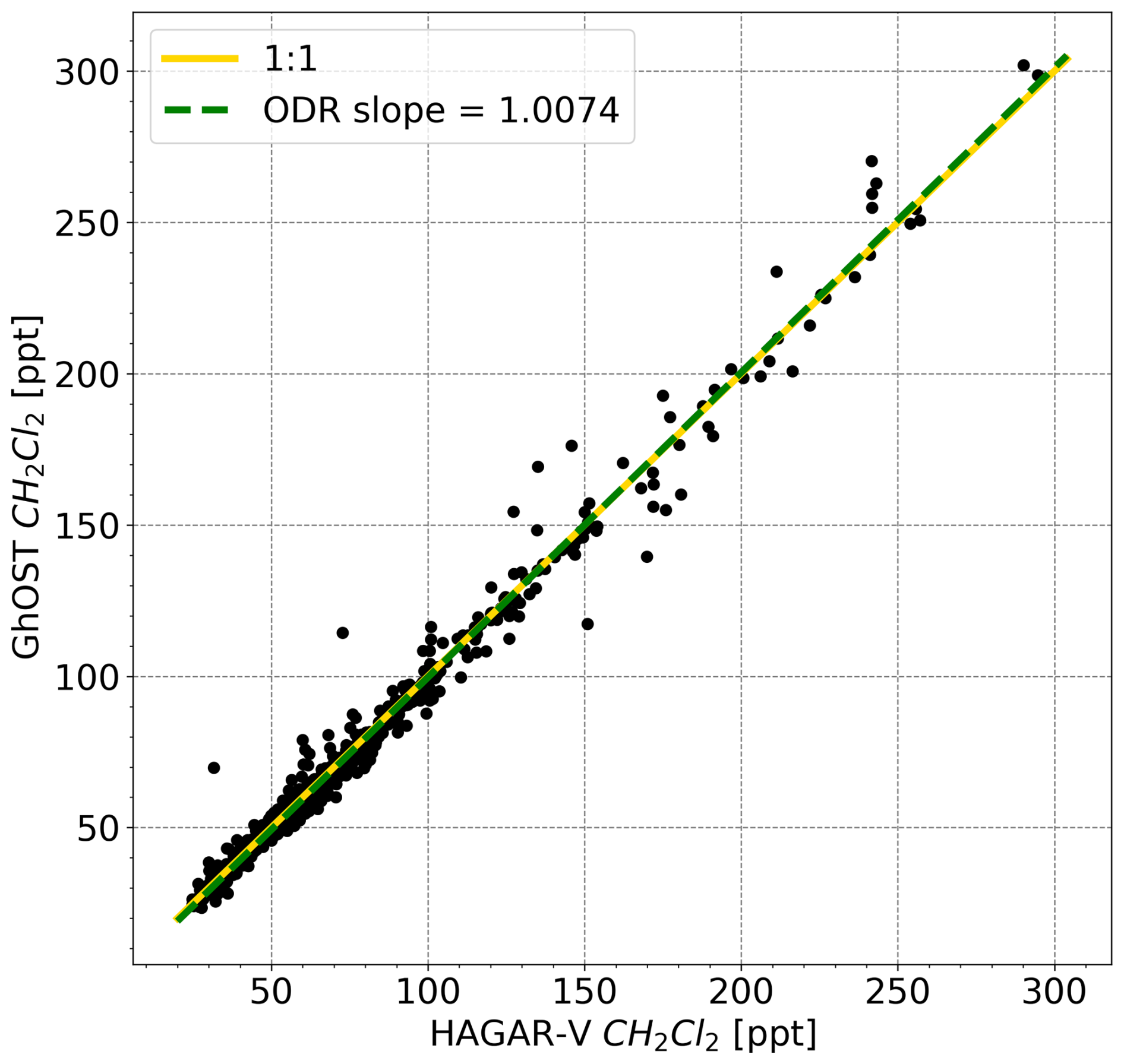
Figure 1 Correlation of CH₂Cl₂ measured with the HAGAR-V instrument (x axis) and the GhOST instrument (y axis). HAGAR-V measurements were averaged when more than one observation was within the sample time of the GhOST instrument. The 1-to-1 line is shown in yellow (solid), and the slope of the orthogonal distance regression is shown in green (dashed).

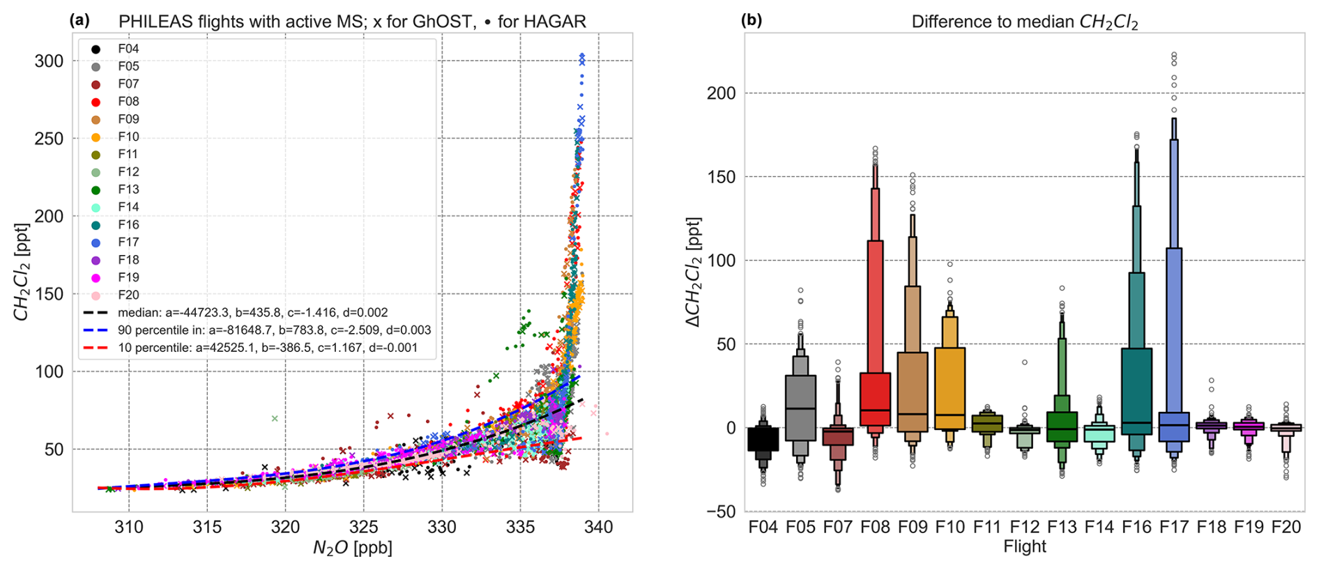
Figure 2 (a) CH₂Cl₂–N₂O relationship, color-coded by flight. Crosses for HAGAR-V and points for GhOST. N₂O is averaged to the respective sample enrichment time of the gas chromatographs. The dashed black curve indicates median curve fit and the dashed blue and red lines the 90th and 10th percentile curve fits. (b) Letter-value plots of ΔCH₂Cl₂ for every PHILEAS flight to median CH₂Cl₂ value derived from median curve fit. Horizontal lines show the median and points extreme outliers.

Using the relationship of CH₂Cl₂ and N₂O (Fig. 2a), periods with considerably increased CH₂Cl₂ without similarly increasing N₂O can be identified. N₂O, a long-lived greenhouse gas, has an atmospheric lifetime of approximately 116 ± 9 years (Prather et al., 2015). It is well mixed throughout the troposphere, and its primary removal mechanism is through photochemical destruction processes in the stratosphere. Furthermore, Fig. 2a shows the median polynomial fit and the 90th and 10th percentile polynomial fit (all polynomials of degree 3), within which 80 % of the observations are located. For mixing ratios below approximately 330 ppb N₂O, a rather compact relationship is observed between N₂O and CH₂Cl₂. Only during flight F07 were several elevated mixing ratios detected by both instruments. For N₂O mixing ratios that are approximately above 330 ppb, a clear partitioning of very high and less pronounced lower values of CH₂Cl₂ can be recognized.

We used the median fit function of the CH₂Cl₂–N₂O relationship to identify the major elevated observations during PHILEAS. For each CH₂Cl₂ observation, we derived a corresponding median CH₂Cl₂ mixing ratio (${\mathrm{CH}}_{\mathrm{2}}{{\mathrm{Cl}}_{\mathrm{2}}}_{\mathrm{med}}$) using the respective N₂O mixing ratio and the median fit function. To more effectively highlight observations that substantially diverge from the median, the deviation (ΔCH₂Cl₂) is determined by subtracting ${\mathrm{CH}}_{\mathrm{2}}{{\mathrm{Cl}}_{\mathrm{2}}}_{\mathrm{med}}$ from the observed CH₂Cl₂ value for each observation. ΔCH₂Cl₂ is displayed as letter-value plots for every flight in Fig. 2b. The plots originate from a central line representing the median. Moving outwards, each subsequent letter layer encompasses half of the residual data, beginning with the 50th percentile that includes 50 % of the data. Following this, the subsequent two segments hold 25 % of the data, continuing this pattern until only outliers are evident. Letter-value plots provide more detailed information in the tails compared to box plots but only where the letter values reliably represent the corresponding quantiles (Hofmann et al., 2011). Four flights stand out where CH₂Cl₂ mixing ratios considerably higher than 100 ppt above ${\mathrm{CH}}_{\mathrm{2}}{{\mathrm{Cl}}_{\mathrm{2}}}_{\mathrm{med}}$ were observed. These are the flights F08, F09, F16, and F17. Three more flights show ΔCH₂Cl₂ between 50 and 100 ppt.

To determine the periods in which extremely high levels (elevated events) of CH₂Cl₂ were observed during the flights, we only consider observations that are above the mixing ratio derived from the fit of the 90th percentile curve and a factor of 2 above the median. In addition, an elevated event must have a duration of at least 10 min without any observation situated between elevated observations that is not itself considered elevated.

The CH₂Cl₂ time series of F08 and F17 are shown in Figs. 3a and 4a with elevated events shaded in red. This work focuses on these two flights. The CH₂Cl₂ time series with elevated events shaded from all four flights (F08, F09, F16, and F17) can be found in the supporting information (Fig. S5). The events in F09 show less coherent structures compared to those of the other three flights. F08 shows a similar high CH₂Cl₂ deviation to F16, but its letter plot tailing towards larger deviations is slightly more pronounced (see Fig. 2b). F17 shows the most pronounced deviation from the median and the overall largest mixing ratios of CH₂Cl₂ measured during the PHILEAS campaign. These two flights show three very clear events with CH₂Cl₂ mixing ratios of 200 to 300 ppt at an altitude of about 11 to 12.5 km and 330 to 350 K potential temperature (Θ) across the northwestern Pacific to the subarctic region of Alaska (Figs. 3b and 4b). In the upper troposphere at comparable potential temperatures, PHILEAS observations within the 10th and 90th percentile ranged from 50 to 80 ppt. Figure 5 displays the flight tracks of these two flights with highlighted segments of the three elevated events.

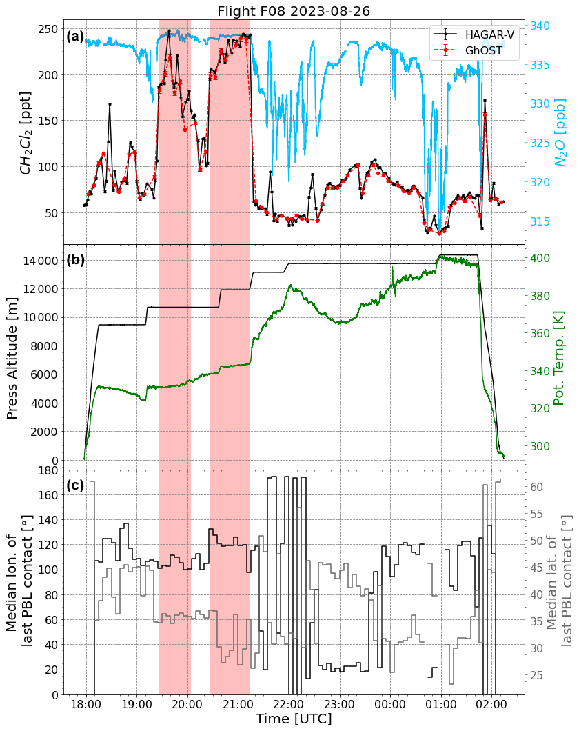
Figure 3 (a) Time series of flight F08 on 26 August 2023. Mixing ratios of CH₂Cl₂ of the GhOST in red and HAGAR-V in black (left y axis) and N₂O in blue (right y axis). (b) Pressure altitude in black and potential temperature in green along the flight path. (c) FLEXPART median latitude in grey and longitude in black of particles within the 5 min intervals. Major elevated time ranges are highlighted in red.

Figure 4 Like Fig. 3 but for flight F17 on 16 September 2023.

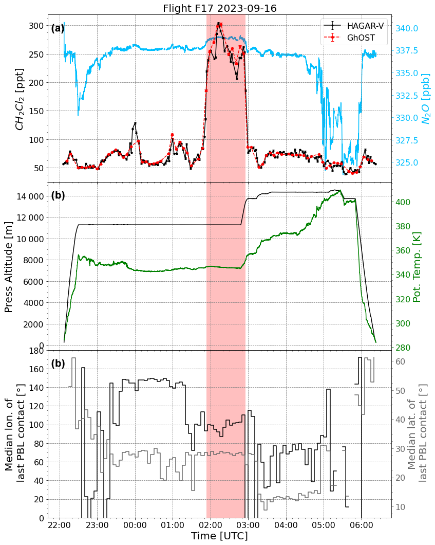
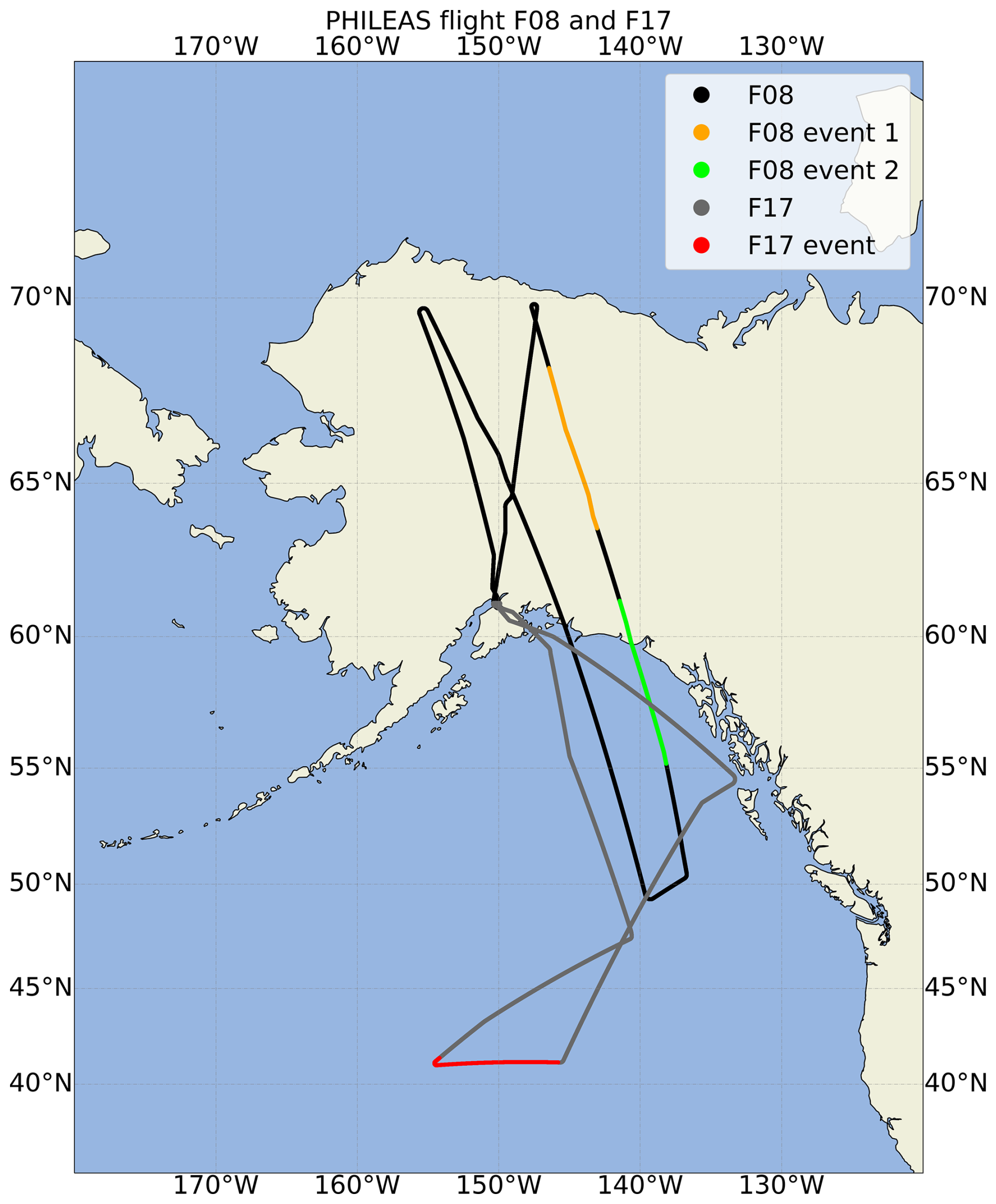
Figure 5 Flight tracks of flight F08 on 26 August (black) and flight F17 on 16 September 2023. Flight segments with high values of CH₂Cl₂ are highlighted in orange, green, and red (F08 event 1, F08 event 2, and F17 event, respectively).

3.3 The origin of elevated CH₂Cl₂ events

To further investigate the origins of the observed elevated CH₂Cl₂ mixing ratios, we utilize the Lagrangian particle dispersion model FLEXPART, running it in backward mode to trace the origins of air masses. Computational air particles, released on the flight path, were followed backward in time until they reached the PBL. Figures 3c and 4c display the median latitude and longitude (only 0–180° E to simplify presentation) of the last PBL contacts of released particles within 5 min intervals along the flight tracks. The backward trajectories indicate a large variability in the median PBL contacts, and the CH₂Cl₂ mixing ratios appear to be sensitive to the last PBL identified by the simulations. This suggests that air masses collected along the flight paths were influenced by various transport histories and were impacted by different source regions.

The two major events of flight F08 exhibit differences in the locations of their most recent PBL contacts. The first event is associated with air masses originating in the longitudinal range of 100–115° E, while the second event is linked to air masses from the 115–130° E region. Furthermore, the first event is more spatially constrained, occurring within the 30–40° N latitude band, whereas the second event encompasses a broader latitude range of around 20–40° N. The event observed during flight F17 illustrates an internal structure of CH₂Cl₂ mixing ratios with a maximum occurring approximately between 02:10 and 02:20 UTC. The calculations of FLEXPART suggest that the last contact of these air masses with the PBL was located over a wide range of longitudes but was restricted to a rather narrow latitudinal band around 30° N.

In both flights, the particles released within the 5 min intervals in the shaded regions of Figs. 3 and 4 show the highest relative proportion of their respective 5 min intervals that have reached the PBL within the 12 d time of our FLEXPART calculation (see Figs. S6 and S7). More specifically, during the first event, the proportions of particle trajectories that have reached the PBL within the prior 12 d are between 50 % and 90 %, while in the second event this figure ranges between 40 % and 50 %. In the F17 event, the relative share exceeds 40 %, with occasional peaks between 60 % and 80 %, which could indicate mixed air masses of different transport pathways. On isentropic levels similar to those associated with the three events, there exist time intervals during these flights when there is an increased percentage of trajectories that reach the PBL as well. However, these trajectories have lower percentages and different median latitudes and longitudes compared to the analyzed events. In the following, we examine the three major events in more depth.

3.3.1 Analysis of the last PBL contacts and the maximum updraft along the trajectories of the events

For each event, we combine the particle trajectories from the 5 min intervals within the event duration, as dictated by the aforementioned conditions and represented by the red-shaded time ranges in Figs. 3 and 4. The initial event occurred on 26 August 2023, from 19:25 to 20:05 UTC, featuring 40 000 particles. The following event on the same day spans 20:25 to 21:15 UTC with 50 000 particles. The final event was observed on 17 September 2023, from 01:50 to 02:50 UTC, with 60 000 particles.

We not only looked at the last PBL contacts of each particle's path, but also conducted an in-depth analysis of regions exhibiting the highest diabatic ascent rates to pinpoint areas of notable updraft along the particles' trajectories during these events. We followed the approach of Hanumanthu et al. (2020) and Lauther et al. (2022) to determine the maximum variation in potential temperature for each particle trajectory over an 18 h period and report the central coordinates for these particles. The focus is on the spatial details of maximum rates along the backward trajectories of the particles rather than on their absolute values. To achieve this, we implemented a rolling window to aggregate the hourly changes in the potential temperature. To better illustrate the findings, the last PBL contacts and the maximum updraft within an 18 h time frame (ΔΘ_18 h) were binned into 2° × 2° latitude–longitude intervals.

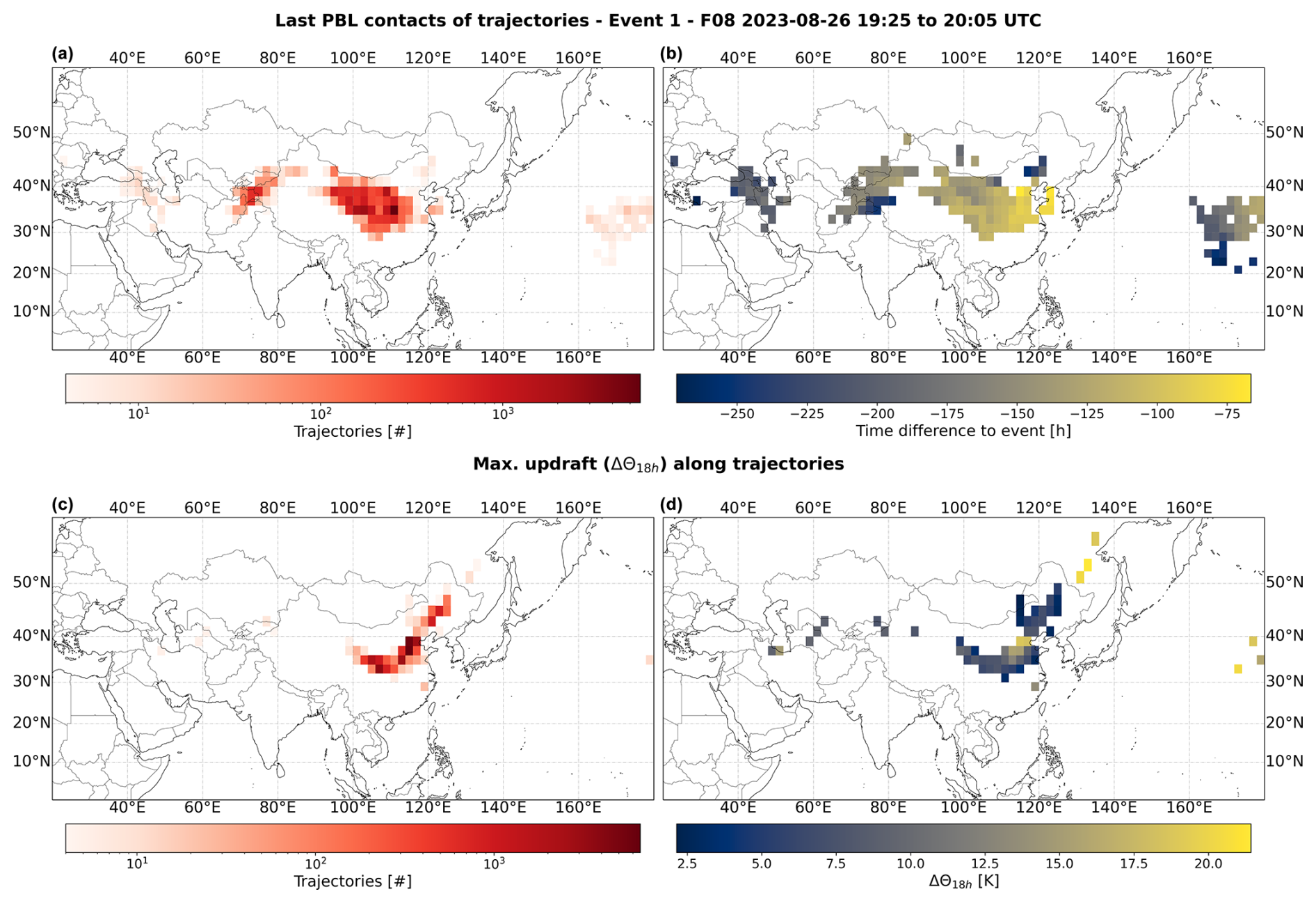
Figure 6 Averaged over 2.0° × 2.0° latitude–longitude intervals for the first event of flight F08, the last PBL contacts and maximum updrafts along the trajectories are shown. Panels (a) and (c) illustrate these intervals, color-coded by the logarithmic scale of trajectory densities for last PBL contacts and maximum updrafts. Panel (b) displays time differences to release time, using color-coded intervals in hours. Panel (d) displays the location of maximum updraft within 18 h along the particle trajectories, color-coded by potential temperature difference within the 18 h.

During the first event on flight F08 on 26 August 2023, almost 80 % of the 40 000 particles (combined 5 min intervals) reached the PBL during the 12 d. Most of the particle trajectories reached the PBL in the Huabei region of northern China, as well as parts of northwest China, including Gansu, Ningxia, and Qinghai provinces. Furthermore, some pathways extended to the far western part of northwest China and the tri-border area of Türkiye, Iran, and Iraq, as well as the Pacific Ocean (Fig. 6a). Transport times to the observation location, particularly from northern China, range from approximately 120 to 144 h (5 to 6 d), with even shorter transport times simulated from trajectories originating in areas near the coast (Fig. 6b). The most intense updrafts are found in northern China near the coastal areas of Hebei, Beijing, and Shanxi (Fig. 6c and d).

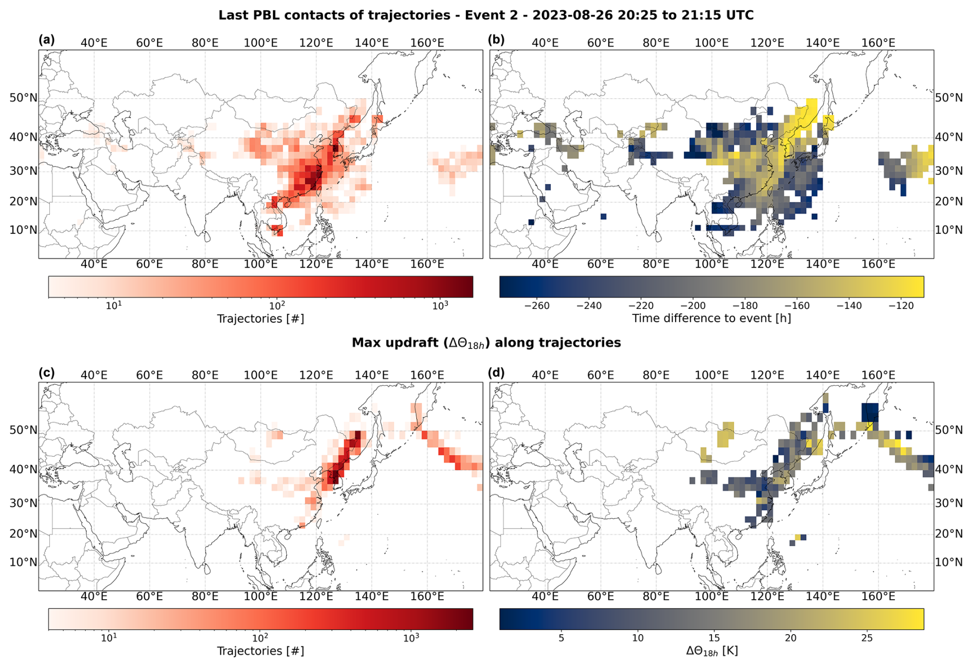
Figure 7 Like Fig. 6, but for the second event on flight F08.

Following the first event on flight F08, the second event was observed soon after, albeit at different isentropic levels. The pattern of the last PBL contacts and the maximum updraft differs somewhat from that of the first event, suggesting that different mechanisms are responsible for the transport. Approximately 40 % of the 50 000 particles reached the PBL during the 12 d of calculation. The most recent PBL contacts are scattered across the Southeast Asia and East Asia regions, as well as somewhat extending into the Pacific Ocean. However, a greater number of trajectories make their last PBL contacts in the Huadong region of East China and the Korean Peninsula (Fig. 7a) with transport times to the observation location ranging from approximately 120 to 168 h (5 to 7 d). Two primary zones show the strongest updrafts along the trajectories: one dense area stretching from the Yangtze River Delta across the Yellow Sea and Korean Peninsula and into Russia's Primorje region and another less concentrated, extending from Kamchatka southeastward over the Pacific Ocean (Fig. 7c). Both regions exhibit comparable updraft intensities (Fig. 7d).

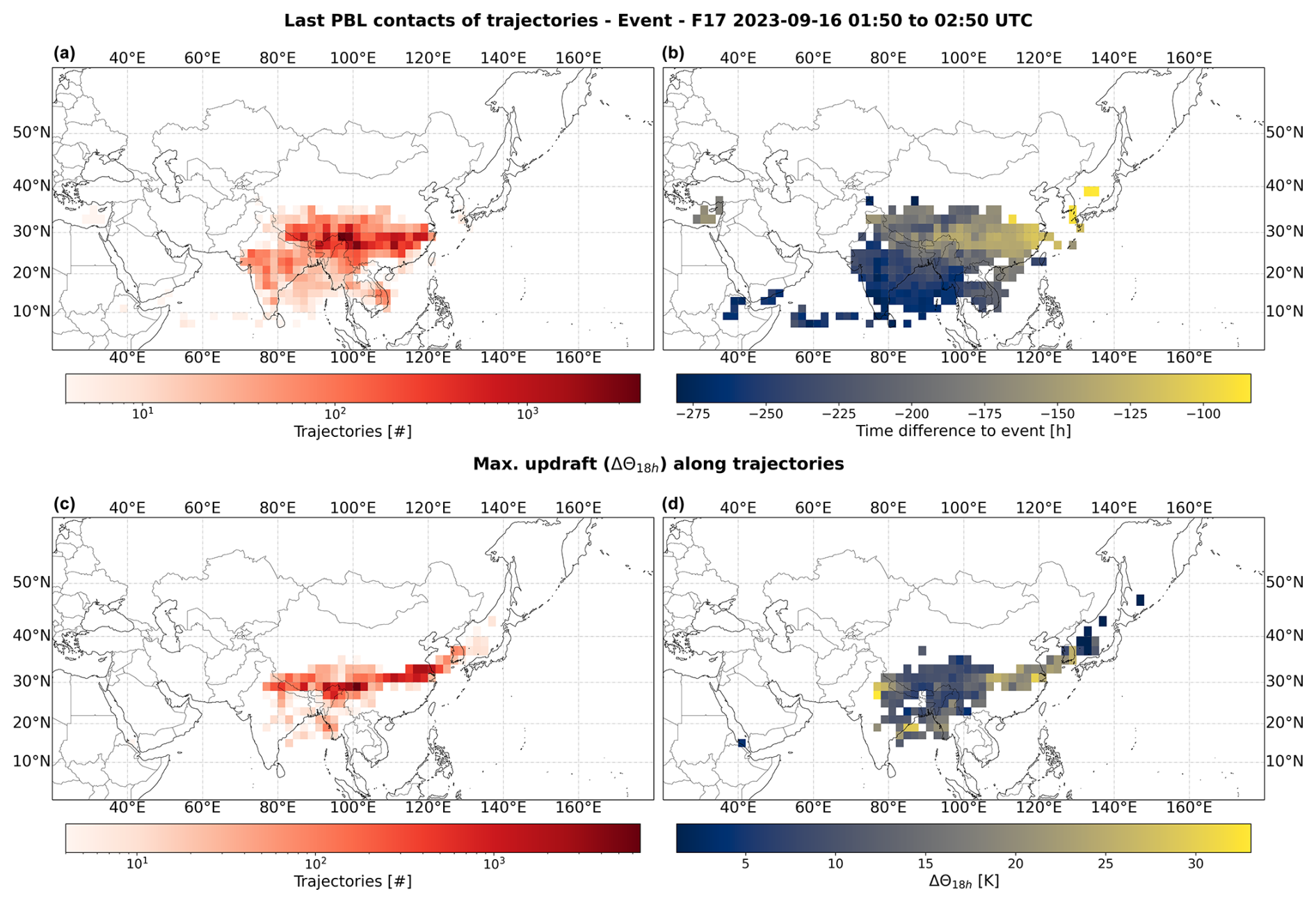
Figure 8 Like Fig. 6, but for the event on flight F17.

The backward calculations for the event on flight F17 on 17 September 2023 display another distinctive pattern of PBL contacts and strongest updrafts compared to the two events on 26 August 2023. Approximately 60 % of the 60 000 particles reached the PBL during the 12 d. Most of the particle trajectories reached the PBL in the more southerly regions of eastern Asia, extending into southern and southeastern Asia. The most recent encounters are located in eastern Asia, particularly closer to the eastern coastal regions, occurring around 120 to 168 h (5 to 7 d) before the flight (Fig. 8a and b). The strongest updraft along the particle trajectories is predominantly confined to a narrow band that stretches from northern India along the southern border of the Tibetan Plateau, passing through Sichuan, Chongqing, Hubei, Anhui, and Jiangsu, and extending to the Korean Peninsula, with the intensity being more pronounced in the area around central to eastern China (Fig. 8c and d).

3.3.2 Synoptic situations and vertical motions

We examined synoptic meteorological conditions that corresponded to the unique patterns of the back trajectories' last PBL contacts and maximum updrafts. ERA5 reanalysis data on pressure levels are provided on an hourly basis. For visualization purposes, only snapshots of the meteorological situation are given, e.g., times with large updrafts. The chosen times roughly coincide with the greatest updraft, based on time series of ΔΘ (potential temperature variation along particle trajectories), visually represented using color codes according to latitude, longitude, and particle density (refer to Figs. S8 to S10). Meteorological fields for periods exhibiting the greatest updrafts are also available in the Supplement (Figs. S15 to S20), together with air mass RGB satellite (EUMETSAT) images for the times of the snapshots (Figs. S11 to S13). Air mass RGB utilizes two water vapor and one ozone absorption channel to differentiate between air masses and high-altitude multi-layered clouds, supporting the examination of dynamic atmospheric processes.

The backward particle trajectories for the first event on flight F08 reveal multiple distinct occurrences of strong updrafts, the most substantial on 22 and 23 August (see Fig. S8). Therefore, we examine two temporal snapshots as depicted in Fig. 9. Figure 9a presents a snapshot from 22 August 2023 at 10:00 UTC of the CAPE parameter. Located within the coordinates of approximately 30–38° N and 110–118° E is a region of enhanced CAPE, thus a region promoting strong and sustained upward air movement. The most substantial period of updraft is on 23 August 2023 at 19:00 UTC for which Fig. 9b shows the Q vector (arrows) and Q-vector convergence (yellow to orange) and divergence (light to dark blue), together with the 500 hPa geopotential (black lines). Positioned at the peak of the updraft along the backward trajectories (see Fig. 6d) is a zone of vertical upward motion, highlighted by the convergence of the Q vector. This is located downstream of a slightly negatively tilted 500 hPa trough, which gradually shifted east over the next few hours (not shown here). Furthermore, this area is located in the entrance region of an anticyclonically curved jet streak (the 200 hPa wind is depicted in Fig. S21), which is related to the vertical upward movement in the troposphere. The closest RGB air mass satellite image at 18:00 UTC shows co-located high-level thick clouds (Fig. S11).

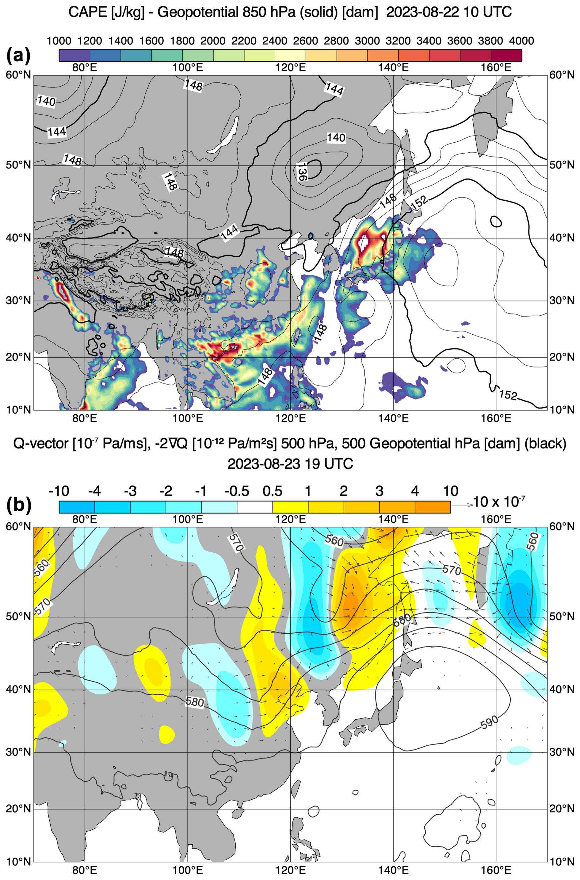
Figure 9 Analysis map from 22 August 2023 at 10:00 UTC (a) and 23 August 2023 at 19:00 UTC (b). Panel (a) shows the vertical distribution of the convective available potential energy (CAPE) and 850 hPa geopotential. Panel (b) shows Q vector, Q-vector convergence or divergence, and 500 hPa geopotential.

For the second event on flight F08, the greatest updraft, noted in the majority of particles involved (Fig. 7c), shows a distinct line from the Yangtze River Delta across the Yellow Sea and the Korean Peninsula and into Russia's Primorje region. The peak period for the potential temperature gradient along the particles occurred from 22 August to early 23 August 2023 (see Fig. S9). Since this appears to be a frontal structure, we utilize the thermal front parameter (TFP) for our investigation. Figure 10a shows large TFP values (yellow to red shadings) located on the warm side of the thickness crowding zone (gradient range of the black lines from shallow to high thickness). This structure remained almost stationary from 22 August 2023 until the early hours of 23 August 2023. The Q-vector convergence implies upward vertical motion for the region of the Yellow Sea, Korean Peninsula, and Russia's Primorje region (Fig. 10b). Moreover, the 500 hPa geopotential chart reveals a detached upper-level low at around 50° N and 120° E. Consequently, this collectively indicates the potential presence of a frontal structure in this area. The RGB air mass satellite image supports this by showing a high-level thick band of clouds along the frontal zone with dark blue to brown colors (cold and dry air) on the rear side (Fig. S12).

Figure 10 Analysis maps from 22 August 2023 at 18:00 UTC. Panel (a) shows the thermal front parameter (TFP) and 850–500 hPa thickness. Panel (b) shows Q vector, Q-vector convergence or divergence, and 500 hPa geopotential.

The event of flight F17 shows again a distinct line of maximum updraft from the Korean Peninsula, across China, and to the southern border of the Tibetan Plateau (see Fig. 8c and d). It is the only one of the three events that indicates an updraft in the SASM monsoon trough region and in the EASM. The monsoon trough region is accompanied by high CAPE values (see meteorological charts in the Supplement). Although strong updraft events occur at several times during the period of the backward calculation, a substantial proportion of particles show their maximum upwind position on a very narrow line within 3 to 6 d prior to their release (see Figs. 8c and S10). Aligned with the strongest updraft area in east China and the Korean Peninsula are large values of the TFP (Fig. 11a), which begin to accumulate on 12 September and dissipate in the early hours of 13 September 2023. Figure 11b illustrates consistent areas of upward vertical motion (Q-vector convergence) near the positively tilted trough in that time. Much like the second event on flight F08, this frontal structure remains largely stationary throughout its duration. An RGB air mass satellite image from 12 September 2023 at 21:00 UTC reveals a thick cloud band, co-located to large values of TFP (Fig. S13).

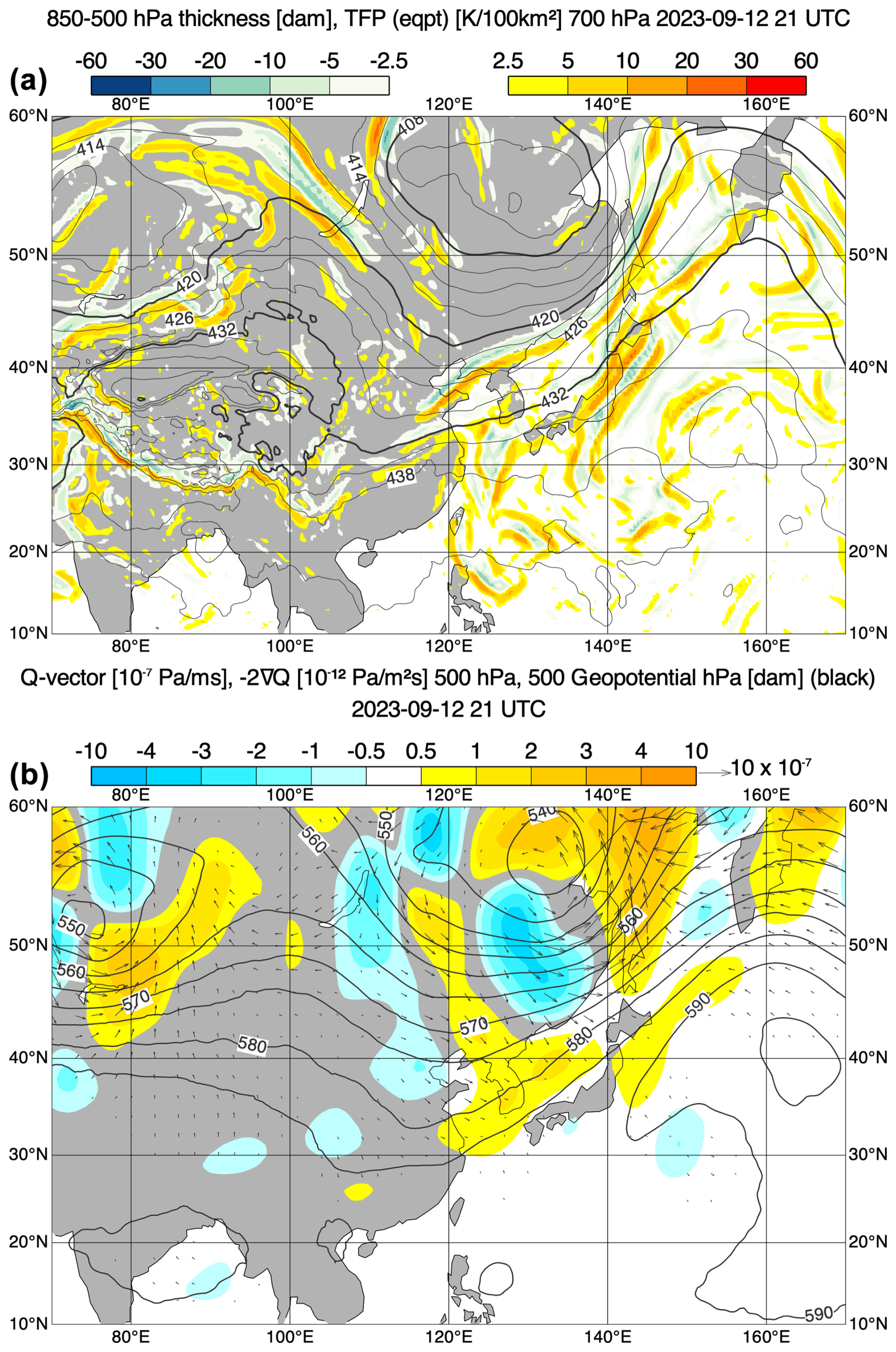
Figure 11 Like Fig. 10, but for 12 September 2023 at 21:00 UTC.

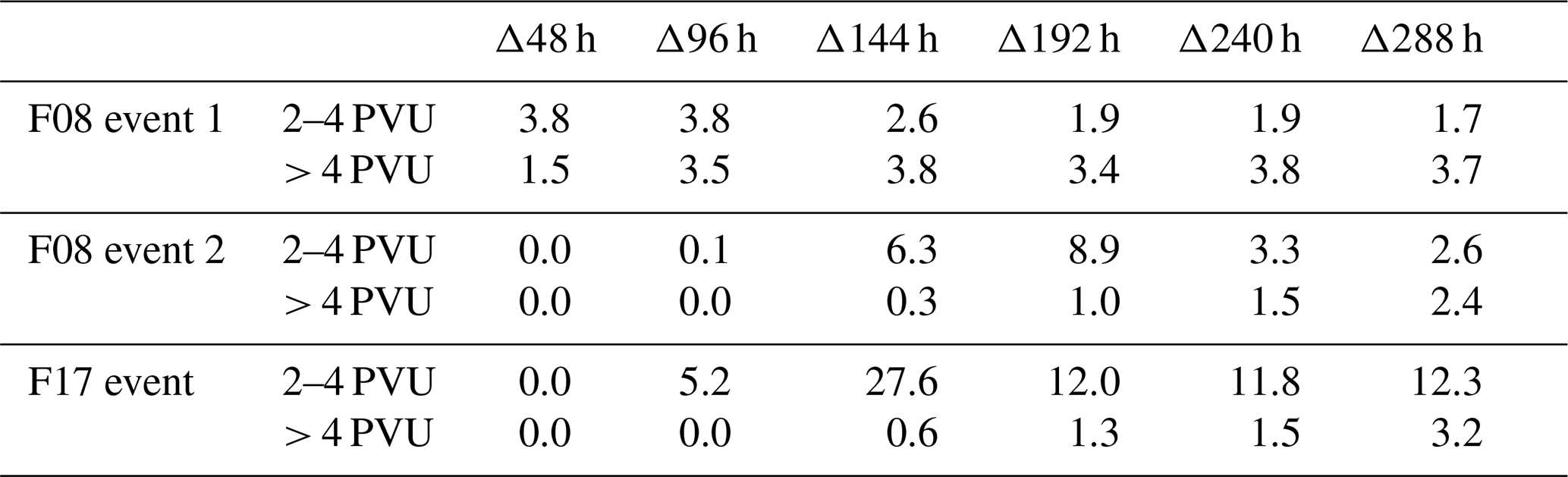
Table 1 Percentage (%) of particle trajectories that are in a potential vorticity range of 2–4 PVU (tropopause region) or greater than 4 PVU (stratospheric), given in 48 h averages along the forward trajectories.

3.4 Projected contribution to the stratosphere

All three events were observed in the upper troposphere at around 330 to 350 K of potential temperature, in proximity to the tropopause and with tropospheric N₂O values (e.g., Figs. 3a, 4a, and S14). To find out whether these air masses with high CH₂Cl₂ can reach further into the stratosphere in the upcoming days, forward particle trajectories were generated. The procedure mirrored that of the backward trajectories, employing 5 min intervals along the flight paths and combining intervals during the event durations. We classify the particle trajectories into three layers based on potential vorticity (potential vorticity unit: PVU). A specific PVU value for defining the dynamical tropopause is not universally established, but 2 PVU is a frequently used threshold (e.g., Holton et al., 1995). Kunz et al. (2009) described the layer where mixing occurs in the tropopause layer as the area that encompasses the dynamic tropopause and thermal tropopause, termed the “tropospheric freshly mixed (TFM)” branch. Furthermore, the lower limit of the TFM branch is established by the dynamical tropopause at 2 PVU, while the mean potential vorticity at the thermal tropopause is estimated to be around 4 PVU. Taking this into account, we utilize the following classification: the first layer is assigned to potential vorticity values below 2 PVU, indicating that it is in the troposphere. The second layer is assigned to values ranging from 2 to 4 PVU, which identifies it as the tropopause layer. The third layer, with values exceeding 4 PVU, is classified as stratospheric. Table 1 shows the percentage share of the ranges 2–4 PVU and greater than 4 PVU (the remaining percentage is below 2 PVU), averaged over 48 h intervals.

All three events demonstrate comparable slight increases in the stratospheric portion with time (> 4 PVU) and exhibit more variations in the share within the tropopause layer (2–4 PVU). In addition, the first event on flight F08 is the only one that shows a minor presence of particles in the tropopause layer and stratosphere within the first 48 h after release.

The first event on flight F08 indicates a minor presence of the particles in the tropopause layer with a decrease within the following days. For the second event on flight F08, the largest share in the tropopause layer was within 7 to 8 d after release at up to 8.9 % with a decreasing contribution afterwards, probably due to the return of some particles to the free troposphere. The largest share to the tropopause layer can be seen for the event on fight F17 at up to 27.6 % on days 5 and 6 with a decreased share in the following days.

The proportion in the stratosphere increases within the 12 d of forward calculation to around 2.4 % and 3.8 % for the three events. For the event on flight F08, the stratospheric proportion exists from the beginning and peaks at 3.8 % after 5 to 6 d. In contrast, for the second event on flight F08 and the event on flight F17, the stratospheric share starts 5 to 6 d after release, reaching its peaks at 2.4 % and 3.2 %, respectively, after 11 to 12 d. The steady increase in particles in the stratosphere within the 12 d could possibly continue in the following days.

4 Discussion

CH₂Cl₂ mixing ratios of up to 300 ppt were observed in the upper troposphere (11–12.5 km) above Alaska and the Gulf of Alaska region. For comparison, observations during take-off and landing at Anchorage show CH₂Cl₂ mixing ratios of about 60 ppt near the ground (see Figs. 3 and 4). We were able to assign the origin of these large mixing ratios to the region of the ASM. We were not the first to observe elevated mixing ratios of CH₂Cl₂ in the upper troposphere even though the focus of previous studies was predominantly on measurements within the ASM or transport in a tropical direction. For instance, Oram et al. (2017) detected CH₂Cl₂ mixing ratios as high as 121 ppt in the upper troposphere (10–12 km) over the Bay of Bengal, originating from East Asia and with potential for transport into the tropical regions of the western Pacific, eventually rising to the tropical upper troposphere. Treadaway et al. (2022) investigated the transport of Asian emissions to the tropical tropopause layer of the west Pacific with a plume of around 90 ppt CH₂Cl₂ (at 14–16 km) with air that originated predominantly from India. Adcock et al. (2021) found tropopause mixing ratios of CH₂Cl₂ in the range of 65–136 ppt in the tropopause region and indicated possible source regions in South Asia. All these studies show enhanced values of CH₂Cl₂ in the upper troposphere and tropopause region but do not reach the values we observed in the upper troposphere in the subarctic area of Alaska. Furthermore, the focus of these studies is on the tropical uplift of elevated CH₂Cl₂ and potential sources from India and South Asia to East Asia. This study mainly examines elevated CH₂Cl₂ mixing ratios originating in the EASM region which were transported to higher latitudes over longer distances. Caution is advised when comparing the absolute values of CH₂Cl₂ with earlier studies, as there has been a notable increase in CH₂Cl₂ emissions over the past decade, rising by a factor of 2.5 (Laube et al., 2022). However, it is clear that the increase in emissions in the region of the EASM is developing much more strongly with considerable importance for transport into the upper troposphere and lower stratosphere.

A more recent study by Pan et al. (2024) not only provides additional evidence for SASM injection of short-lived ozone depleting substances, but also highlights the key role of EASM in injection into the stratosphere. During the ACCLIP campaign, an unusual northward shift in the convergence zone was observed due to an atypical configuration of the ASM for that year. Typically, the convergence zone is positioned slightly more southward. However, both in 2022 and climatologically, the convergence zone intersects with significant Cl-VSLS sources along the coastal regions of East Asia (Pan et al., 2024).

Our findings support this statement, as our backward trajectories for three substantial CH₂Cl₂ plume observations in the upper troposphere revealed the last PBL contacts in known source areas of CH₂Cl₂ and peak updrafts suggest predominantly typical line structures which can be associated with frontal structures and convergence zones (also visible in RGB air mass satellite images in the Supplement). This highlights once more the importance of viewing the EASM as a key pathway for transporting Cl-VSLSs into the upper troposphere, thereby contributing to an increase in tropospheric background levels with the potential to enter the lower stratosphere. Moreover, the transport times and areas of increased CH₂Cl₂ mixing ratios shown here suggest that transport to the upper troposphere in the subarctic region is driven by large convective transport contributions from the EASM. Previous studies have focused more on the entry of polluted air into the UTLS via the ASMA with subsequent eddy-shedding events. The ASMA covers a range of potential temperatures from approximately 360–450 K (see, for example, Vogel et al., 2019). Small-scale eddies are shed from the main anticyclone (i.e., the so-called eddy-shedding events) with quasi-horizontal isentropic transport out of the anticyclone, either directly into the lower stratosphere or into the tropical troposphere with subsequent slower transport into the stratosphere (e.g., Clemens et al., 2022). Elevated CH₂Cl₂ mixing ratios were identified in a potential temperature range of 330–350 K in this study, thus below the ASMA.

Typical frontal structures in the EASM region include the Meiyu, Baiu, and Changma fronts, where the name changes with the location of the frontal structure. As the monsoon progresses, the structures shift northward. They first appear over Taiwan, southern China, and the Okinawa region from early May to mid-June. They then move to the Yangtze River valley and the main islands of Japan from mid-June to mid-July and finally reach the Korean Peninsula and northeast China during mid-July to mid-August (e.g., Jun-Mei et al., 2013). In this study, frontal structures were observed at the end of August. Shin et al. (2022) investigated the synoptic characteristics of the quasi-stationary front of August 26–27 2018 over the Korean Peninsula, similar to the frontal structure within this study. The quasi-stationary front observed in their study exhibited features similar to the Changma front. The environmental conditions of the August event examined were atypical for heavy rainfall with a quasi-stationary front and are closely related to the expansion of the subtropical high of the west Pacific (WPSH) (Shin et al., 2022). This study also observed an expansion of the WPSH, occurring not just in late August but also in mid-September accompanied by frontal structures.

We conducted a preliminary analysis of the potential for elevated CH₂Cl₂ occurrences to penetrate deeper into the tropopause layer and lower stratosphere. The ongoing challenge is to mitigate stratospheric ozone depletion caused by the increasing trend of uncontrolled Cl-VSLSs (Chipperfield and Bekki, 2024). The forward trajectory analysis indicates varied contributions for the three events. For the tropopause layer, the contribution fluctuated significantly between events, reaching approximately 25 % during the largest event. All three events show a minor contribution to the lower stratosphere up to about 3.8 % within the 12 d period following the events. We are considering a specific time frame and geographic region, while other regions may have a greater impact on transportation into the stratosphere. For instance, transport can occur in the ridges of baroclinic waves on the anticyclonic side of the jet stream, situated above the outflow of warm conveyor belts (e.g., Kunkel et al., 2019).

5 Summary and conclusion

We report on measurements of CH₂Cl₂ from two in situ instruments and N₂O from a third in situ instrument during the HALO aircraft campaign PHILEAS in late summer 2023. One of the primary scientific interests centered on how polluted air from the Asian Summer Monsoon region reached the extratropical upper troposphere and lower stratosphere (UTLS), with research flights mainly originating from Anchorage, Alaska. In addition, the FLEXPART Lagrangian dispersion model was used to investigate the origin of selected pollution events, the corresponding transport times from the planetary boundary layer (PBL), and the potential for further input into the lower stratosphere, using calculations extending 12 d both backward and forward.

The measurements of CH₂Cl₂ recorded by the two in situ instruments align very well. Major pollution events during the PHILEAS campaign were identified by examining the relationship between CH₂Cl₂ and N₂O. Two flights (F08 and F17) showed three very clear events with CH₂Cl₂ mixing ratios of 200 to 300 ppt at altitudes of about 11 to 12.5 km and 330 to 350 K potential temperature over the northwestern Pacific up to the subarctic region of Alaska. These mixing ratios deviate substantially from the comparable median mixing ratios of the campaign.

The FLEXPART model in backward mode was used to trace the origins and transport times of air masses responsible for elevated mixing ratios observed during the aforementioned pollution events. For each event, the paths of the computational air particles were analyzed to identify the last PBL contacts and regions of maximum diabatic ascent using potential temperature variations along particle trajectories. Transport times between PBL and the flight paths for the three events were around 5–7 d. For the first event on flight F08, the particle trajectories reached the PBL primarily over northern China (approximately 30–40° N and 100–115° E), with updrafts focused closer to coastal areas. For the second event on flight F08, the particle trajectories, which reached the PBL, dispersed across Southeast Asia and East Asia (approximately 20–40° N and 115–130° E). The updrafts were notably strong along the Yangtze River Delta, over the Korean Peninsula, and extending into Russia. For the event on flight F17, the particle trajectories reached the PBL in broader region of southern to southeastern Asia (approximately 20–30° N and 80–120° E). Updrafts were concentrated from northern India to eastern China and the Korean Peninsula.

ERA5 reanalysis was used to identify meteorological conditions such as frontal structures and vertical motions that aligned with particle trajectory patterns and updraft intensities. Key findings indicated distinct patterns in each event, influenced by regional meteorological conditions such as convective areas and frontal structures, revealed through parameters such as CAPE, Q-vector divergence, and the thermal front parameter (TFP). RGB air mass satellite images were used to confirm the presence of frontal structure with associated cloud formations.

This analysis of the elevated CH₂Cl₂ mixing ratios indicates that the transport into the upper troposphere in the subarctic region resulted from convective upwelling by the EASM and subsequent displacement over the northern Pacific Ocean before the air masses could ascend further into the ASMA and be subsequently transported into the lower stratosphere.

By forward FLEXPART calculation of the three events, the potential of these observed elevated CH₂Cl₂ mixing ratios to reach the tropopause layer and lower stratosphere in the following days (12 d time period) was investigated. Even if a substantial proportion reaches the tropopause layer (up to 27.6 % for flight F17), the contribution to the lower stratosphere is minor for all three events (1.3 % to 3.8 %). However, it remains unclear whether this observation is limited to the events we observed or if it extends more generally to convection within the East Asian part of the monsoon circulation. More detailed and systematical investigation is needed to determine this.