Lagrangian coherent structures to examine mixing in the stratosphere

The study of mixing in the stratosphere is important for understanding the transport of chemical species and the dynamics of the atmosphere. How best to quantify this mixing is not settled, however. In recent years, Lagrangian coherent structures (LCSs) have emerged as a valuable tool for examining mixing in fluid flows, and in this work, we present a stratospheric mixing metric based on the LCS framework. We identify LCSs associated with the transport of air masses and quantify the amount of mixing between different regions of the atmosphere in the Whole Atmosphere Community Climate Model (WACCM). Our results show that LCSs provide a powerful approach to analyze mixing in the stratosphere and can be used to identify regions of high and low mixing as well as to study the dynamics of the atmosphere. The results are compared with those obtained by two other tools to quantify mixing: the commonly used effective diffusivity and the recently introduced isentropic eddy diffusivity. We find qualitative agreement between these metrics for much of the stratosphere, although there are regions where they clearly disagree. A significant advantage of the LCS mixing metric is that it reflects Lagrangian transport in physical latitude rather than the equivalent latitude coordinate needed to calculate effective diffusivity, and we discuss other advantages and disadvantages of these methods.

1 Introduction

The stratospheric circulation shapes the distribution of trace gases in the stratosphere, including ozone, water vapor, and ozone-depleting substances (Butchart, 2014). This circulation can conceptually be separated into two components: the slow meridional overturning circulation and the fast quasi-horizontal mixing. These are not independent – the breaking of planetary-scale waves drives both – but the timescales are sufficiently different that the separation is physically meaningful. Metrics that quantify the stratospheric circulation typically employ this separation by timescale. The meridional overturning circulation is often characterized with the vertical velocity in the transformed Eulerian mean (TEM) circulation (Andrews and McIntyre, 1976) or less frequently with the diabatic circulation (Pyle and Rogers, 1980; Rosenfield et al., 1987; Linz et al., 2017a), which is very similar to the TEM vertical velocity calculated from radiative heating rates (Linz et al., 2019). Methods for calculating the quasi-horizontal mixing have less consensus, with mixing being characterized by a Lagrangian effective diffusivity (Nakamura, 1996; Haynes and Shuckburgh, 2000; Abalos et al., 2016a) or with a box model (Neu and Plumb, 1999; Ray et al., 2010, 2016), using Lyapunov diffusivity (Shuckburgh et al., 2009; d'Ovidio et al., 2009), using Lagrangian diffusivity (Curbelo and Mechoso, 2024; LaCasce, 2008), using vertical gradients of the ideal age tracer (Linz et al., 2021; Gupta et al., 2023), or even as a residual in the age tracer budget (Garny et al., 2014; Ploeger et al., 2015a, b).

The balance between the slow overturning and the fast quasi-horizontal mixing determines the distributions of trace gases. For example, lower-stratospheric midlatitude ozone is affected by mixing of ozone-poor air from the tropics and downward transport of ozone-rich air from above (e.g., Hegglin and Shepherd, 2007; Neu et al., 2014). This lowermost stratospheric region is important for air quality and for climate; it is the reservoir of stratospheric air from which air is transported into the troposphere via stratospheric intrusions (Shapiro, 1980; Holton et al., 1995), and ozone is a particularly strong greenhouse gas in this region. Analysis of tracers in models shows that they have relatively similar representations of the strength of the overturning circulation but very different mixing strength (Dietmüller et al., 2018). Likewise, although future ozone changes due to advection are somewhat consistent in models, the ozone changes due to differences in eddy mixing changes are much more uncertain both because of the processes and because of the methods to calculate mixing terms (Abalos et al., 2020).

Chaotic advection describes a situation in which a spatially smooth and periodic or quasiperiodic time-dependent velocity field produces irregular particle trajectories (Aref, 1984; Ottino, 1989). This definition can be generalized in a natural way to temporally aperiodic kinematic flows such as stratospheric flows (Malhotra and Wiggins, 1998): chaotic mixing and transport are mediated by the lobes formed by the stable and unstable manifolds (Wiggins, 1992) and explained using hyperbolicity concepts associated with attracting and repelling lines, as well as hyperbolic zones with strongly chaotic behavior. Therefore, a necessary condition for chaotic advection in dynamical flows is that there exists an “organizing structure” (which includes stagnation points) for mixing and transport Ngan and Shepherd (1999). This framework for studying fluid transport and mixing is often referred to as the “dynamical systems approach to Lagrangian transport” since the focus is on understanding the organizing structures in phase space for fluid particle trajectories (Ottino and Wiggins, 2004; Samelson and Wiggins, 2006; García-Garrido et al., 2018)

There is strong evidence for the existence of such spatial structure in the stratosphere. Waugh and Plumb (1994) and Norton (1994) showed that small-scale tracer structure in the stratosphere is determined mostly by the large-scale flow. This behavior is consistent with the so-called Rossby wave critical-layer paradigm (e.g., Juckes and McIntyre, 1987), which states that the forced Rossby wave critical layer provides a useful conceptual model for the stratospheric surf zone (Haynes and McIntyre, 1987; Salby and Garcia, 1987; Bowman, 1996). Several authors (e.g., Bowman, 1993; Waugh and Plumb, 1994; Schoeberl and Newman, 1995) have shown that particle trajectories in the surf zone are chaotic.

According to Ottino (1989), fluid mixing can be conceptualized as the effective stretching and folding of material lines and surfaces. Even turbulent flows feature Lagrangian structures that can be understood from the perspective of finite-time dynamical systems theory (Shadden et al., 2005). This has led to the development of the theory of Lagrangian coherent structures (LCSs) (Haller, 2015). A LCS is a distinguished surface within a dynamical system, like fluid flow, that significantly influences the behavior of nearby trajectories over a specific time interval. LCSs play a crucial role in shaping global transport and act as transport barriers by serving as key material surfaces. These finite-time structures are the most relevant structures in time-dependent flows, as they determine the deformation of the fluid and the evolution of any advective tracer field. The concept of LCSs was introduced by Haller and Yuan (2000). Attracting hyperbolic LCSs are lines that evolve with the flow and attract fluid to the greatest extent. In the vicinity of these attracting LCSs, the fluid is stretched in one direction and compressed in the other direction, making them the cores of filamentous tracer patterns. The application of LCSs to the stratosphere has the potential to provide new insights into the mechanisms controlling the transport and mixing of chemical species.

This paper introduces the density of Lagrangian coherent structures as a new metric for stratospheric mixing and compares it to two different stratospheric mixing metrics: the more commonly used effective diffusivity (Nakamura, 1996) and the newer tracer-based isentropic eddy diffusivity (Gupta et al., 2023). Although effective diffusivity is commonly used, its calculation is computationally expensive, and results are in the somewhat ambiguous equivalent latitude coordinate. As we show in Sect. 3.3.1, latitude and equivalent latitude are not (name notwithstanding) truly equivalent. The density of LCSs does not solve the problem of computational expense, but it is a Lagrangian metric that nevertheless provides results in physical latitude.

We also compare to the isentropic eddy diffusivity, a metric based on the eddy transport of the idealized tracer age of air and the mean meridional gradient in age of air (Gupta et al., 2023). Age of air describes how long an air parcel has been in the stratosphere since entering at the tropopause, and so age reflects the average of the Lagrangian pathways of the bits of air that make up a larger air parcel. At each location, there is more accurately an age spectrum that describes the distribution of times different parts of the air parcel have taken to reach the current point (Hall and Plumb, 1994). Mean ages in the stratosphere reach over 5 years, and so the computational burden of using age is due to model equilibration time. Age of air, more than any other tracer, reflects Lagrangian transport. The isentropic eddy diffusivity is calculated from age transport and is implicitly a Lagrangian metric.

We introduce the density of LCS as a mixing metric, not with the suggestion that it is superior to these other methods, but with the idea that it provides a different and hopefully useful perspective on stratospheric mixing.

The paper is organized as follows: in Sect. 2, we describe the data and methods used in our analysis. In Sect. 3, we apply the proposed metric (Sect. 2.2) to characterize mixing and present our results, while also comparing its use to the other metrics defined in Sect. 2.3 and 2.4. We present our conclusions and discuss both limitations and potential avenues for future research in Sect. 4.

2 Methods

2.1 Model simulation

The study utilized a comprehensive climate model, the Community Earth System Model 1 Whole Atmosphere Community Climate Model (WACCM), which is identical to the one used in Linz et al. (2021) and Gupta et al. (2023). This interactive chemistry–climate model (Garcia et al., 2017; Marsh et al., 2013) was developed at the National Center for Atmospheric Research (NCAR) and incorporates physical parameterizations to simulate complex Earth system processes, such as atmospheric chemistry and radiation. It is based on a finite-volume dynamical core (Lin, 2004) from the Community Atmosphere Model version 4 and covers a domain from the surface to 140 km, with 31 pressure levels (Neale et al., 2013). The model has a horizontal resolution of 2.5° longitude ×1875° latitude, corresponding to the F19 horizontal grid. The WACCM simulations were based on the Chemistry Climate Model Initiative REF-C1 scenario (Morgenstern et al., 2017) and forced with observed sea surface temperatures. The Quasi-Biennial Oscillation was nudged to observed winds, but, otherwise, the model evolved freely. The model was integrated from 1979, and additional information on WACCM is provided in Sect. 3 of Linz et al. (2021).

The selection of WACCM instead of reanalysis products is due to comparison purposes: the calculation of isentropic eddy diffusivity requires a high-temporal-resolution spatially resolved age of air (AoA) field, which this particular WACCM run provides. Such a product is quite rare, with monthly mean zonal mean being the norm, and reanalysis products usually do not offer this. In addition, WACCM ensures internally consistent physics.

2.2 Lagrangian descriptor

The approach is based on the Lagrangian descriptor called the M function (Mancho et al., 2013). By analyzing trajectories in both the forward and backward directions, this technique can categorize trajectories with analogous qualitative characteristics. The expression for the M function is

$$\begin{array}{}\text{(1)}& {\displaystyle }{\displaystyle }M({\mathit{x}}_{\mathrm{0}},t_{\mathrm{0}},\mathit{\tau })=\underset{t_{\mathrm{0}}-\mathit{\tau }}{\overset{t_{\mathrm{0}}+\mathit{\tau }}{\int }}\Vert \mathit{v}\left(\mathit{x}\right(t;{\mathit{x}}_{\mathbf{0}}),t)\Vert \mathrm{d}t,\end{array}$$

and it corresponds to the arc length of the trajectory traced by a fluid parcel starting at x₀=x(t₀) as it evolves forwards and backwards in time with velocity v(x,t) for a time interval $(t_{\mathrm{0}}-\mathit{\tau },t_{\mathrm{0}}+\mathit{\tau })$. This tool already has been widely used to visualize LCS in atmospheric flows (de la Cámara et al., 2012; Manney and Lawrence, 2016; Curbelo et al., 2017, 2019a, b, 2021; Niang et al., 2020).

LCSs are often used to study mixing in fluid flows because they can be used to identify regions of the flow where there is a high degree of mixing and regions where there is little mixing. In particular, regions where LCSs are closely packed together or highly curved are associated with strong mixing, while regions where LCSs are far apart or relatively straight are associated with weak mixing.

Although using a τ parameter that varies with the constant potential temperature level would provide a more accurate representation, as radiative timescales indeed differ between the upper and lower stratosphere, we chose to use a constant τ throughout the stratosphere for this study, as it serves as an initial proof of concept for our method. We consider this a reasonable approximation for the purposes of our analysis. For this study, we set τ=15 d and focused on levels above 400 K, where the effect of varying timescales is less pronounced. The calculation of M depends on the choice of τ, and for stratospheric studies, several articles indicate that τ=15 d yields reliable results (de la Cámara et al., 2012; Curbelo et al., 2017, 2019a, 2021; Manney and Lawrence, 2016). Since our focus is on climatological studies of the zonal mean, the sensitivity to this parameter is negligible.

To measure mixing based on the notion that higher spatial occurrence of LCS leads to greater mixing, we have developed a diagnostic tool that relies on the probability density function (PDF) of LCS presence across each time for a given latitude, longitude, and isentropic level.

The algorithm works as follows: for each instant (data every 3 h) and isentropic level of the wind velocity, we calculate M using Eq. (1) and then determine the LCS as the ridges of the gradient of M, $\Vert \mathrm{\nabla }M\Vert$, following Curbelo et al. (2019a, 2021); i.e., the locations of LCSs in maps of M correspond to abrupt spatial changes in the descriptor, which are identified by large values of normalized $\Vert \mathrm{\nabla }M\Vert$, i.e., those in the top 30 % of their range after normalization by their maximum value. We then calculate the PDF in the corresponding time interval, i.e., the entire study period (2007–2009), or the corresponding seasons or subsets of interest for each specified latitude, longitude, and altitude. Finally, we compute the zonal average of this quantity, which is shown in the upper row of Fig. 2 for the climatological period of 2007–2009 (Fig. 2a), for December–January–February 2007–2009 (DJF, Fig. 2b), and June–July–August 2008–2009 (JJA, Fig. 2c). This map displays the locations where coherent structures are most prevalent (in yellow), indicating higher levels of chaotic advection, in contrast to areas where their presence is lower (dark blue). We acknowledge that the dynamics of mixing in the atmosphere are far more complex. As highlighted by d'Ovidio et al. (2009) and Shuckburgh et al. (2009), less intense waves can still contribute to more efficient mixing due to their specific interactions with stable and unstable manifolds, where the angle of intersection plays a critical role. Our metric does not pretend to replace existing models but instead serves as a complementary tool for understanding stratospheric mixing under a wider range of conditions. For example, if the output from a coarse-resolution model precludes accurate calculations of mixing, not because the model fails to represent mixing well, but because the method requires higher resolution, then a different method is needed. LCS density is not the only possible solution to this problem, but due to the properties of its Lagrangian approach, it can be applied across a wide range of resolutions (see Badza et al., 2023, for more information on LCS and uncertainties in data).

Figure 1 shows snapshot of $\Vert \mathrm{\nabla }M\Vert$ at 600K for several days of 2008.

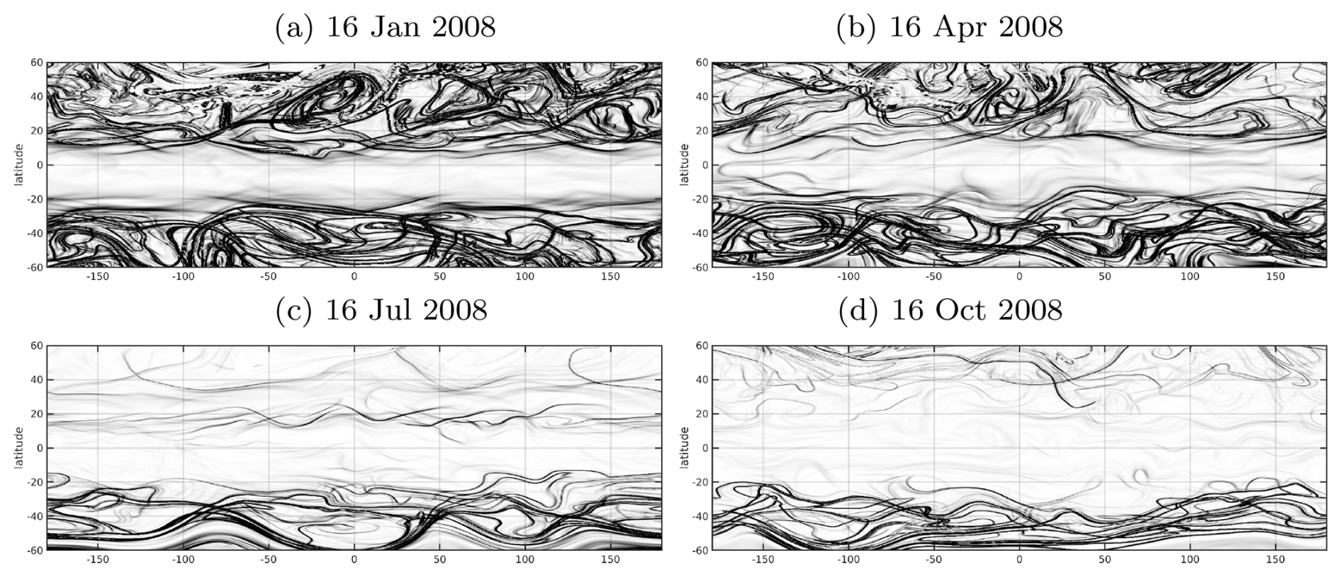
Figure 1 Snapshot of $\Vert \mathrm{\nabla }M\Vert$ for different days of the year 2008 at 600 K. In the maps, black lines correspond to large values of $\Vert \mathrm{\nabla }M\Vert$, that is, approximately the LCSs.

By considering that a higher quantity of LCS correlates with increased mixing, we can infer from Fig. 1 that the midlatitudes have greater mixing than the Equator and tropics, with variations also apparent due to seasonal differences.

Note that it is not necessary to take the zonal mean. LCS density can be used to look at the full three-dimensional structure of stratospheric mixing (see Shuckburgh et al., 2009). For comparison with other metrics of mixing, however, the zonal mean is the most appropriate.

Previous studies have explored the spatial structure of mixing using both dynamical and tracer-based metrics. We compare our new diagnostic tool with another Lagrangian tool, effective diffusivity, and the implicitly Lagrangian isentropic eddy diffusivity from age of air.

2.3 Effective diffusivity

The effective diffusivity represents the degree of intricacy or elongation of tracer contours as they are transported by the non-divergent isentropic wind field. This method, which is based on a Lagrangian treatment of mixing and transformation of equations based on tracer-area coordinates, has been used by Nakamura (1996), Shuckburgh et al. (2001), and Abalos et al. (2016a) among others to quantify mixing in the atmosphere. Following Haynes and Shuckburgh (2000), the effective diffusivity κ_eff in equivalent latitudes ϕ_e is defined by

$$\begin{array}{}\text{(2)}& {\displaystyle }{\displaystyle }{\mathit{\kappa }}_{\text{eff}}({\mathit{\varphi }}_{\mathrm{e}},t)=\mathit{\kappa }{\displaystyle \frac{L_{\text{eq}}^{\mathrm{2}}({\mathit{\varphi }}_{\mathrm{e}},t)}{(\mathrm{2}\mathit{\pi }R\cos {\mathit{\varphi }}_{\mathrm{e}}{)}^{\mathrm{2}}}},\end{array}$$

where L_eq is the equivalent length of a tracer contour, the diffusivity κ is a constant, and R is the Earth's radius. The equivalent latitude ϕ_e is defined by $A=\mathrm{2}\mathit{\pi }{R}^{\mathrm{2}}(\mathrm{1}-\sin {\mathit{\varphi }}_{\mathrm{e}}$), with A being the area of the region for which the tracer concentration is greater than or equal to the tracer contour Q. By using equivalent latitude as an independent variable, the advective terms in the tracer concentration evolution equation are eliminated. This means that the effective diffusivity κ_eff only characterizes the tracer's diffusion with respect to the contours of ϕ_e.

The second row of Fig. 2 shows the effective diffusivity in equivalent latitude coordinates ϕ_e vs. isentropic coordinates θ. To compute Eq. (2) we use as a tracer the potential vorticity (PV), and we follow the calculations of Haynes and Shuckburgh (2000). Regions characterized by high values of effective diffusivity (in yellow) demonstrate strong mixing, causing tracer contours to be extensively stretched.

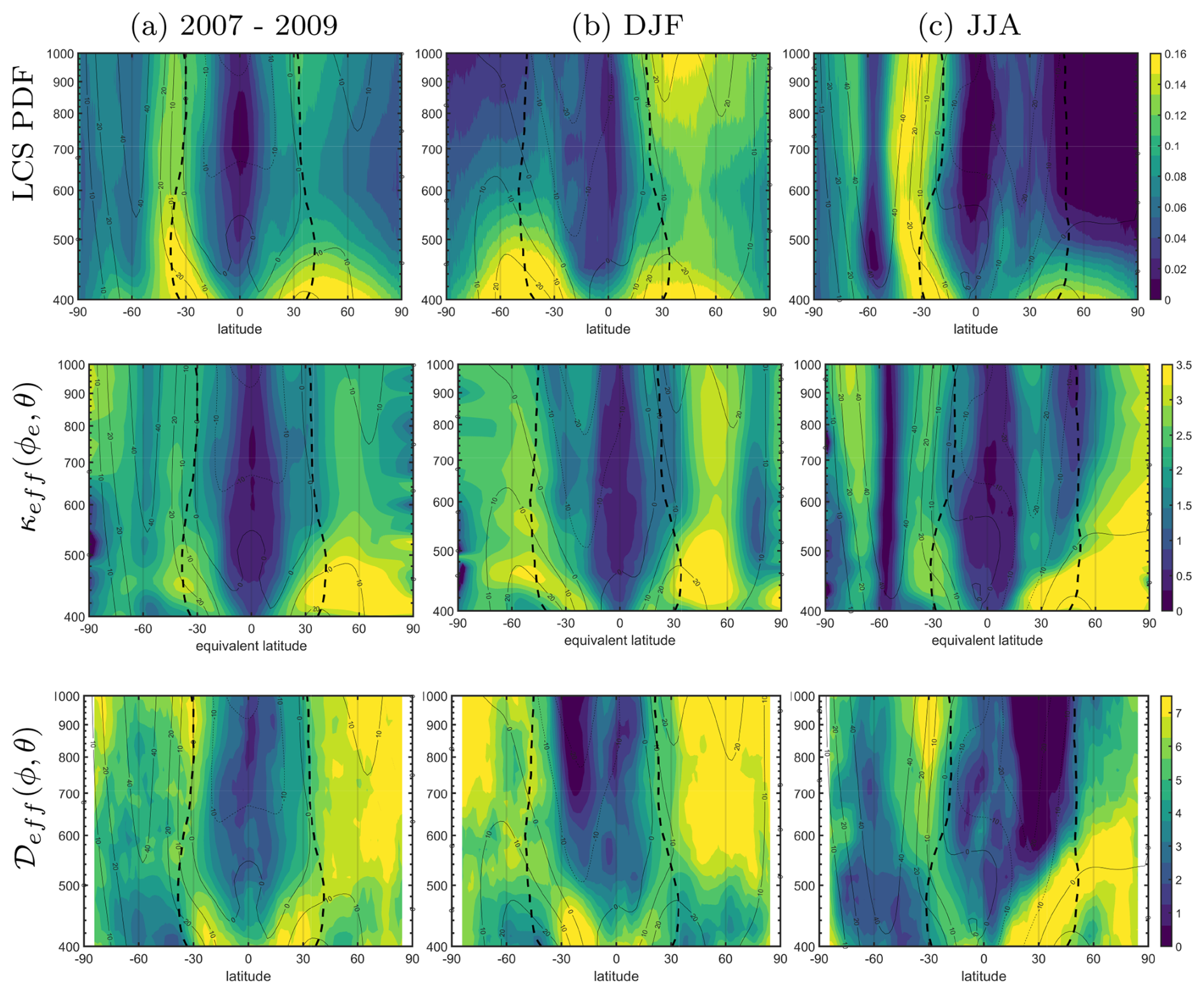
Figure 2 Density of LCS, defined as the zonal mean of the probability density function of LCS presence (first row). Effective diffusivity κ_eff(ϕ_e,θ) distribution (second row) and isentropic eddy diffusivity 𝒟_eff(ϕ,θ) (third row), averaged over each day during the years 2007–2009. (a) Climatology of 2007–2009; (b) DJF 2007–2009; (c) JJA 2007–2009. The dashed black line is the zero diabatic velocity curve, i.e., $\dot{\mathit{\theta }}=\mathrm{0}.$ This line is a function of ϕ and θ. The thin lines correspond to the zonal mean zonal wind.

2.4 Isentropic eddy diffusivity

An alternative approach to evaluate the meridional distribution of the mixing flux is through the isentropic eddy diffusivity. Eddy tracer fluxes have been used in the past to examine mixing (e.g., Plumb and Mahlman, 1987; Abalos et al., 2016b), and the version of this calculation we think is most relevant for comparison to our LCS metric is the one used in Gupta et al. (2023) because it is based on age of air. Age of air, Γ, is a measure of how long an air parcel has been in the stratosphere, and age has a spatially independent source (of 1 yr yr⁻¹) within the stratosphere, with a boundary condition of zero at the tropopause (Hall and Plumb, 1994; Waugh and Hall, 2002). Age represents the integrated paths of the bits of air that make up a larger parcel, and so we expect age to be more closely related to the Lagrangian perspective than other tracers. The isentropic eddy diffusivity 𝒟_eff (units of m² s⁻¹), calculated from age and following the notation of Gupta et al. (2023), is the ratio of the net eddy transport of age to the mean meridional age gradient and is defined by

$$\begin{array}{}\text{(3)}& {\displaystyle }{\displaystyle }{\mathcal{D}}_{\text{eff}}={\displaystyle \frac{\mathrm{1}}{{\stackrel{\mathrm{‾}}{\mathit{\rho }}}_{\mathit{\theta }}}}{\displaystyle \frac{-F_{\text{eddy}}}{{\partial }_y\stackrel{\mathrm{̃}}{\mathrm{\Gamma }}}},\end{array}$$

with $\stackrel{\mathrm{̃}}{\mathrm{\Gamma }}(\mathit{\varphi },\mathit{\theta })=\stackrel{\mathrm{‾}}{{\mathit{\rho }}_{\mathit{\theta }}\mathrm{\Gamma }}/{\stackrel{\mathrm{‾}}{\mathit{\rho }}}_{\mathit{\theta }}$ being the mass-weighted age in isentropic coordinates, ρ_θ the isentropic density, v the meridional velocity, ${\partial }_y=(\mathrm{1}/R){\partial }_{\mathit{\varphi }}$ the meridional gradient of the mean isentropic age, and F_eddy the eddy age flux in isentropic coordinates given by

$$\begin{array}{}\text{(4)}& {\displaystyle }{\displaystyle }{F}_{\text{eddy}}(\mathit{\varphi },\mathit{\theta })=\stackrel{\mathrm{‾}}{{\mathit{\rho }}_{\mathit{\theta }}v\mathrm{\Gamma }}-\stackrel{\mathrm{‾}}{\left({\mathit{\rho }}_{\mathit{\theta }}v\right)}\stackrel{\mathrm{̃}}{\mathrm{\Gamma }}.\end{array}$$

Here the overbar denotes zonal averaging on fixed isentropes. The eddy diffusivity given by 𝒟_eff is expected to have its highest value in the midlatitudes of the stratosphere due to the strong eddy transport induced by planetary waves and the weak meridional gradients in the surf zone. Consequently, the isentropic eddy diffusivity can be utilized as a qualitative measure to evaluate the midlatitude eddy mixing structure. The isentropic eddy diffusivity defined by Eq. (3) for the same period as previous tools is shown in the lowermost row of Fig. 2.

3 Results

3.1 Relation between the stratospheric circulation and the presence of Lagrangian coherent structures

To better understand the results of using the new LCS metric for mixing, first we briefly review some characteristics of the stratospheric circulation, its seasonal cycle, and what might be expected for the seasonal cycle of stratospheric mixing. Much of this explanation is based on Plumb (2002) and Butchart (2014), and we highlight the characteristics most relevant to understanding mixing. The large-scale stratospheric circulation is driven by the breaking of planetary-scale Rossby waves that propagate upwards from the troposphere. These waves can be caused by land–sea contrast, flow over topography, or the interactions of synoptic-scale eddies. Waves can propagate vertically only in appropriate background winds, and the appropriateness of the winds is dependent on the zonal wavenumber (Charney and Drazin, 1961). The summer hemisphere has mean easterly winds above the lower part of the stratosphere, prohibiting deep vertical propagation of Rossby waves. We thus expect waves to break in the lower stratosphere in the summer hemisphere and the upper part of the stratosphere to be relatively quiescent. The winter hemisphere, in contrast, has climatological westerly winds that are typically of a strength that allows zonal wavenumbers 1–2 to propagate vertically into the middle and upper stratosphere (waves with zonal wavenumbers 3–4 still break in the lower stratosphere). If we consider that wave breaking is associated with horizontal mixing, we thus expect to see strong mixing in the lower stratosphere in both hemispheres and mixing in the winter hemisphere throughout the depth of the stratosphere. Other features that are important are the subtropical mixing barriers (the so-called tropical pipe Plumb, 1996; Neu and Plumb, 1999) and the polar vortex. The polar vortex is a band of strong westerly winds at about 60° latitude in the winter hemisphere, and these winds are well known as a mixing barrier (e.g., Mitchell et al., 2021).

The new metric based on the presence of LCS is calculated for the period of 2007–2009, and the annual average and the solstice seasons are shown in the top row of Fig. 2. Here, the dashed black lines represent the turnaround latitude in each hemisphere, that is, the latitude associated with zero diabatic velocity $\dot{\mathit{\theta }}=\mathrm{0}$. The turnaround latitude can have a varying latitude with height and time. The region bounded by the two dashed black lines, known as the tropical pipe, exhibits a gradual diabatic ascent of mass. Similarly, the area located toward the poles, encompassed by the black curves, is characterized by a slow diabatic descent of mass. These two divisions are referred to as the upwelling and downwelling regions, respectively. In DJF, the Northern Hemisphere has a greater and stronger circulation, and the upwelling region extends into the Southern Hemisphere. The maximum in LCS density is poleward of the diabatic circulation minimum but equatorward of the vortex edge. This suggests the greatest mixing is occurring in the surf zone between these two barriers. Similarly, in JJA, the Southern Hemisphere exhibits a stronger circulation, and the upwelling area extends into the Northern Hemisphere, with the highest values of LCS density around 30° S, just poleward of the southern turnaround latitude.

Figure 2 shows regions of low LCS density include the regions at the core of the polar jets, with the lowest values in the SH polar jet in JJA around 60° S. There is a gradient from the highest values of LCS density in the midlatitudes to lower values near the subtropical mixing barriers. The lowest LCS density is then found at the Equator, suggesting very little mixing happening within the deep tropics (5° S–5° N) in either season. This is consistent with the picture shown in the snapshots in Fig. 1, where there are almost no strong gradients in M right at the Equator. Our findings for the tropics are consistent with the effective diffusivity results from Abalos et al. (2016a) (more below), who point out that this is to be expected because of known weak mixing within the tropical pipe (Plumb, 1996).

3.2 LCS density diagnostic in longitude–latitude

Longitude–latitude sections of the LCS density at various isentropic levels for both DJF and JJA 2007–2009 are shown in Fig. 3. The levels are all in the stratospheric overworld (400 K and above). Generally, there is less mixing at the Equator and more mixing poleward, and these sections show the same characteristics as the zonal means, with the upper stratosphere having mixing (more LCS density) in the winter hemisphere, while the lower stratosphere has mixing in both.

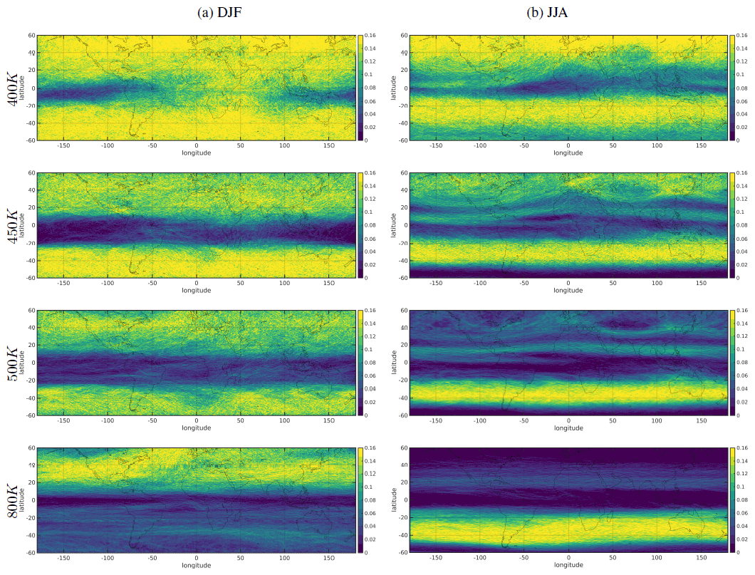
Figure 3 Longitude–latitude map of LCS density at 400, 450, 500, and 800 K. (a) DJF 2007–2009; (b) JJA 2007–2009.

Clear longitudinal differences are visible in all potential temperature levels, though DJF has more zonal symmetry than JJA. This demonstrates the potential of this technique for comparing key features of the stratospheric circulation, such as the location of polar vortices, jets, and regions of wave breaking. The effect of the Asian monsoon can also be seen by looking at the latitude–longitude maps of the LCS density. This boreal summertime feature is especially prominent at 450 and 500 K. By 800 K, its influence is not seen, and at 400 K, we surmise that there are other wave-breaking signatures that make the monsoon relatively less important.

Large-scale atmospheric circulation patterns, particularly the Asian monsoon anticyclone, play a significant role in stratospheric mixing, driving exchanges between the subtropical and midlatitude lower stratosphere with significant impacts on chemistry (e.g., Solomon et al., 2016). During the summer months, the monsoon-induced circulation can facilitate strong meridional transport and enhance mixing, independent of wave activity. There is extensive literature on the influence of the monsoon anticyclone on stratospheric composition and its role in stratospheric mixing (e.g., Dethof et al., 1999; Ploeger et al., 2013). The monsoon is the primary entry point for many substances into the stratosphere (Randel et al., 2010), including constituents that are important for ozone (Adcock et al., 2021; Liang et al., 2025), and so the mixing barriers near the anticyclone have important implications for the distribution of anthropogenic pollutants in the stratosphere.

3.3 Comparison between density of LCSs and effective diffusivity

A comparison of the three metrics used to describe diffusion and mixing, effective diffusivity, LCS density, and isentropic eddy diffusivity is shown in Fig. 2. Our discussion of the features is somewhat modeled on the work of Abalos et al. (2016a), whose presentation of effective diffusivity is excellent.

In the region above the subtropical jets, the most intense mixing occurs in the middle latitudes of the lower stratosphere during the summer. This mixing pattern extends to higher altitudes during the austral (December–February) summer than the boreal (June–August) summer. In the winter lower stratosphere, the mixing is constrained to a narrower latitudinal band due to the presence of the lower portion of the polar vortex. This is especially true for the Southern Hemisphere.

The evolution as a function of latitude for the effective diffusivity and the LCS density is shown in Fig. 4 on four selected isentropic levels: 400 (the lower part of the stratospheric overworld region), 450, 500, and 800 K (lower, middle, and high stratosphere). For consistency with the calculation of LCS where we use a time interval τ=15 d, here we also apply a 15 d running mean to instantaneous diffusivity. Both metrics show characteristics in common: minimum values are observed in the core of the polar jets in both hemispheres and in the tropics, following the latitudinal displacement of the tropical easterlies towards the summer hemisphere. In the middle stratosphere, mixing gradually increases at the edge of the vortex during late winter and spring, persisting until approximately 1 month after the breakdown.

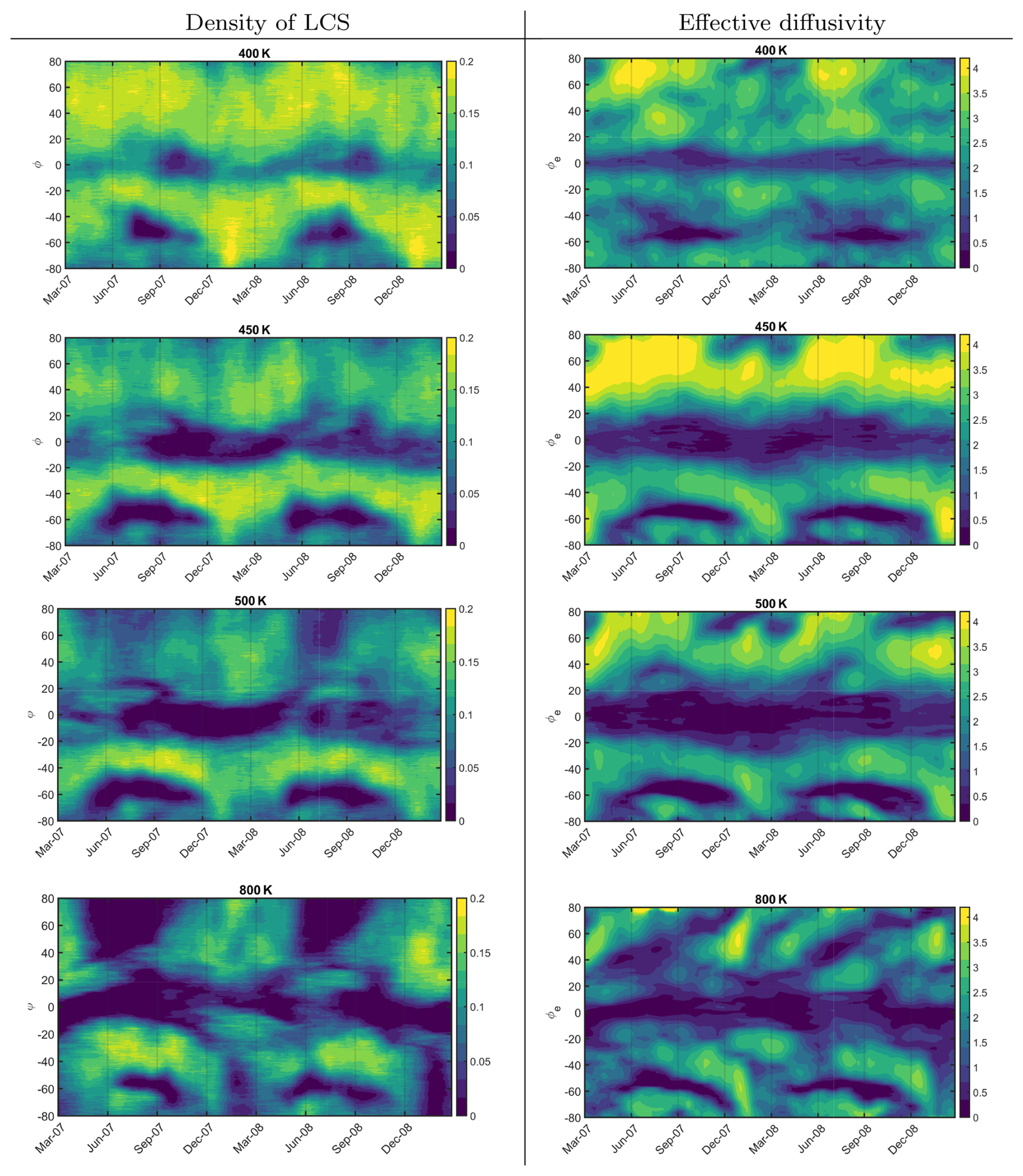
Figure 4 Diffusivity distribution using our new diagnostics tool (LCS density, first column) and effective diffusivity (second column) for 2 years (March 2007 to February 2009) on the 400, 450, 500, and 800 K isentropic surfaces. A 15 d running mean has been applied to the instantaneous diffusivity.

Seasonal evolution in the Northern Hemisphere reveals notable differences. At 450 K, effective diffusivity peaks around 40–50° N, while LCS indicates weaker summertime mixing, consistent with expectations based on wave breaking. In contrast, the seasonal cycle of effective diffusivity intensifies at higher altitudes, showing stronger summertime mixing at 800 K. Notably, effective diffusivity exhibits a pronounced seasonal cycle, particularly at 800 K.

There is also a difference in relative magnitudes of apparent mixing lower and higher in the stratosphere, with LCS showing a stronger gradient between 400 and 800 K. This could be real and reflect a difference in wave breaking that is better captured with the LCS, or it could be related to the choice of a constant τ at all levels. A lower τ is appropriate for looking at tropospheric variability, for example. All levels here are within the stratosphere, but we perform no optimization for choosing τ, and so this choice could introduce a bias.

Figure 5 highlights the temporal evolution of the diffusivity for equivalent latitude of 50° N on the same isentropic levels as Fig. 4. This emphasizes that the seasonality very present when using the LCS density in the middle stratosphere is lost in the case of using the effective diffusivity (see the yellow and purple curves corresponding to 500 and 800 K, respectively). A strong seasonal cycle in mixing is expected because of the seasonality of wave breaking. Thus, the lack of a strong seasonal cycle in effective diffusivity suggests the metric may be lacking. We hypothesized that this may be related to the seasonality in equivalent latitude, which we now investigate.

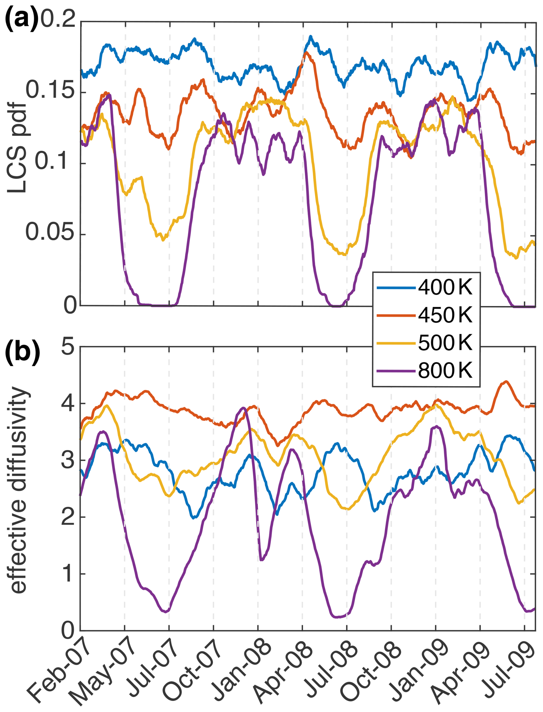
Figure 5 (a) Distribution of LCS at ϕ=50° N and (b) effective diffusivity distribution at ϕ_e=50° N for January 2007 to July 2009 on the 400, 450, 500, and 800 K isentropic surfaces. A 15 d running mean has been applied to the instantaneous diffusivity.

3.3.1 Equivalent latitude

The utilization of equivalent latitude specifically derived from contours of potential vorticity (PV) has become a widely accepted method for analyzing the transport of air masses on isentropic surfaces within the stratosphere and upper troposphere (Allen and Nakamura, 2001, 2003; Allen et al., 2012; Nakamura, 2024). However, employing equivalent latitude based on potential vorticity (PV) as a horizontal coordinate has some limitations (Allen and Nakamura, 2003; Pan et al., 2012). Firstly, the calculation of PV involves intricate mathematical manipulations of observed or assimilated winds and temperature, resulting in the introduction of noise due to the convolution of analysis errors (Newman et al., 1989). Although this noise does not significantly affect the equivalent latitude overall, it can be amplified at specific locations and times when PV gradients are weak. Secondly, the resolution of PV is constrained by the resolution of the underlying wind and temperature fields, whose data quality decreases with altitude, making PV notably noisier in the upper stratosphere (Manney et al., 1996). To address these problems, several authors have developed alternative methods for generating high-resolution maps of equivalent latitude for tracer analysis (Allen and Nakamura, 2003; Haynes and Shuckburgh, 2000; Anel et al., 2013).

The utilization of equivalent latitude coordinates also presents other complications because of the seasonal cycle of PV or whatever tracer is chosen to calculate equivalent latitude. Therefore the effective diffusivity mixing results in equivalent latitude may not be directly comparable to mixing metrics in latitude. We are not claiming an inherent issue with equivalent latitude as a concept, as it is invaluable for stratospheric studies. The details of its calculation matter quite significantly, however. In order to understand the effect of the use of coordinate systems based on equivalent latitude in the definition of diffusivity, we examine equivalent latitude from PV: its temporal evolution, mean, and standard deviation.

The standard deviation of the equivalent latitude for each isentropic level and PV contour values Q is defined as

$$\begin{array}{}\text{(5)}& {\displaystyle }{\displaystyle }\mathit{\sigma }(Q,\mathit{\theta })=\sqrt{{\displaystyle \frac{\mathrm{1}}{N-\mathrm{1}}}\sum _{i=\mathrm{1}}^N\left|{\mathit{\varphi }}_{\mathrm{e}}^i(Q,\mathit{\theta })-\stackrel{\mathrm{‾}}{{\mathit{\varphi }}_{\mathrm{e}}}(Q,\mathit{\theta })\right|},\end{array}$$

where N is the number of observation (d), ${\mathit{\varphi }}_{\mathrm{e}}^i(Q,\mathit{\theta })$ is the corresponding latitude value of the area enclosed by the closed contour Q on the level θ at time t_i, and $\stackrel{\mathrm{‾}}{{\mathit{\varphi }}_{\mathrm{e}}}(Q,\mathit{\theta })$ is the time mean:

$$\begin{array}{}\text{(6)}& {\displaystyle }{\displaystyle }\stackrel{\mathrm{‾}}{{\mathit{\varphi }}_{\mathrm{e}}}(Q,\mathit{\theta })={\displaystyle \frac{\mathrm{1}}{N}}\sum _{i=\mathrm{1}}^N{\mathit{\varphi }}_{\mathrm{e}}^i(Q,\mathit{\theta }).\end{array}$$

To simplify the notation, we relate the Q contour that depends on the isentropic level to the temporal mean of the equivalent latitude on that surface, that is, we take ${\mathit{\varphi }}_{\mathrm{e}}\equiv \stackrel{\mathrm{‾}}{{\mathit{\varphi }}_{\mathrm{e}}}(Q,\mathit{\theta })$ and therefore $\mathit{\sigma }({\mathit{\varphi }}_{\mathrm{e}},\mathit{\theta })\equiv \mathit{\sigma }(Q,\mathit{\theta })$.

Figure 6 shows the temporal evolution of the equivalent latitude for each potential vorticity contour value at four different potential temperature levels θ=400, 450, 500, and 800 K. The last panel of this figure illustrates the changes in the equivalent latitude, ϕ_e, associated with a given value of potential vorticity, Q, across different isentropic levels and over time. It reveals regions where ϕ_e remains nearly constant (near the Equator), in contrast to other regions where significant differences are observed. Low latitudes show little variability, while higher latitudes show seasonal and interannual variability. The strong seasonal cycle in the PV contour associated with a given equivalent latitude suggests that the seasonal cycle in effective diffusivity could be related to the seasonal evolution of the coordinate system. Effectively, by using equivalent latitude, we are imposing the seasonal cycle of PV onto the mixing metric.

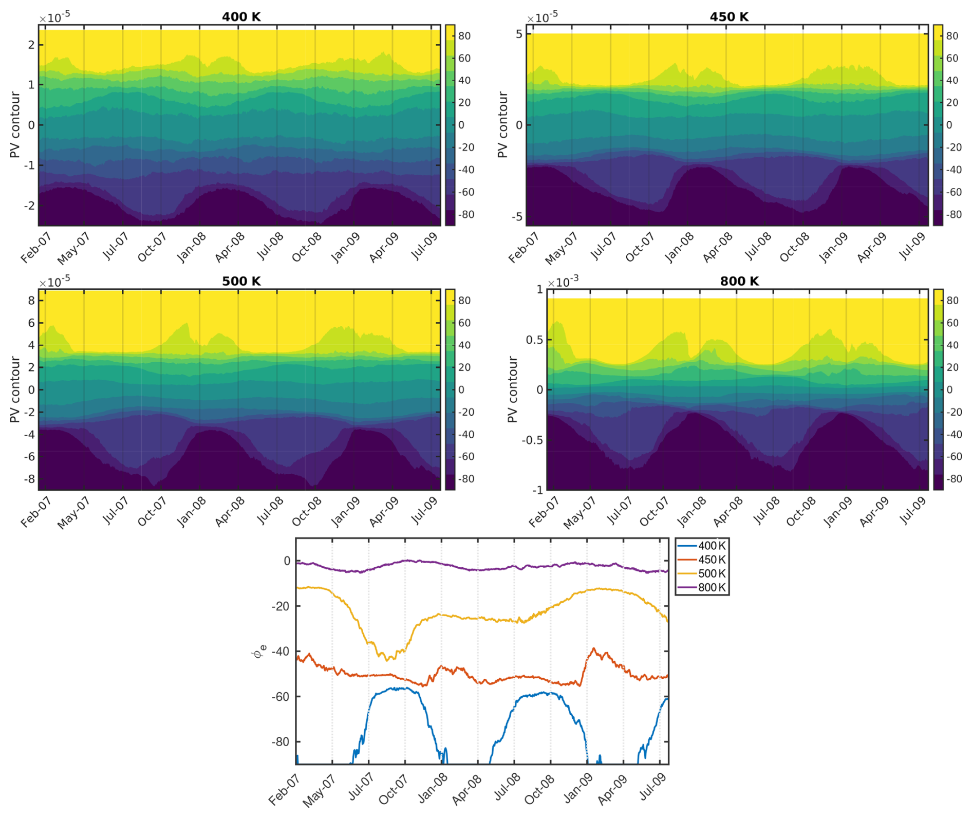
Figure 6 The equivalent latitude ϕ_e as a function of time t and PV contour Q (ϕ_e(Q,t)) for the isentropic level 400, 450, 500, and 800 K. Last panel shows the time evolution of ϕ_e for $Q=-\mathrm{2}\times {\mathrm{10}}^{-\mathrm{5}}{\mathrm{m}}^{\mathrm{2}}{\mathrm{s}}^{-\mathrm{1}}\mathrm{K}{\mathrm{kg}}^{-\mathrm{1}}$ on these θ levels.

Note that latitude is a geographical coordinate, whereas equivalent latitude is a tracer-contour-based coordinate that represents the latitude at the edge of a polar cap enclosing the same area as a given tracer contour. In other words, it corresponds to the area enclosed by a specific tracer contour. We focused on equivalent latitude as a coordinate for defining effective diffusivity, κ_eff, but a more general perspective based on tracer contour areas provides a clearer interpretation. Equivalent latitude is inherently tied to the chosen tracer, and since different tracers can exhibit distinct seasonal cycles, the seasonality of κ_eff depends on the tracer itself rather than solely on the choice of equivalent latitude as a coordinate. Figure 6 is equivalent to plotting the time-evolving PV as a function of ϕ_eq (i.e., remapping one as a function of the other); therefore, the seasonal cycle of ϕ_eq in PV coordinates is the same as the seasonal cycle of PV in ϕ_eq coordinates. That is, the seasonal cycle of equivalent latitude in PV coordinates mirrors the seasonal cycle of PV in equivalent latitude coordinates. However, this dependence on seasonality is not unique to equivalent latitude; any tracer-based coordinate system will reflect the seasonal variability of the chosen tracer. Therefore, κ_eff, when computed using PV as a tracer, naturally inherits the seasonal cycle of PV regardless of the coordinate system used. This highlights the importance of considering the tracer's intrinsic variability when interpreting κ_eff. Potential discrepancies in κ_eff calculations may also arise as a result of the specific data, model, or scheme employed to compute the PV field (Abalos et al., 2016a; de la Cámara et al., 2018).

Equivalent latitude is very useful for characterizing stratospheric dynamics, as demonstrated by numerous studies. This is particularly true for comparing different in situ observations within the same season but at different times or different years (e.g., Ray et al., 2024), and there are many good reasons to use equivalent latitude in the stratosphere, especially for the polar regions (see, e.g., Allen and Nakamura, 2003).

To examine the seasonal effect further, Fig. 7a shows the standard deviation of the equivalent latitude following this definition (Eq. 5) for the JJA season 2007–2009. The standard deviation is compared with effective diffusivity (Fig. 7b), density of LCS (Fig. 7c), and isentropic eddy diffusivity (Fig. 7d). Large values of standard deviation of equivalent latitude coincide with the regions where the greatest differences between the three metrics are found, i.e., in the Southern Hemisphere between 50–20° S and in the Northern Hemisphere at lower isentropic levels and inside the band of 40–20° N for higher isentropic levels. This last region is particularly interesting because, despite the fact that κ_eff shows large values of diffusivity here, the other metrics, which do not use ϕ_e, show much lower diffusivity values (LCS density) or even indicate non-existent diffusivity in the area as in the case of 𝒟_eff. This is a region where relatively few waves can propagate and break, and so low values are more consistent with the wave forcing.

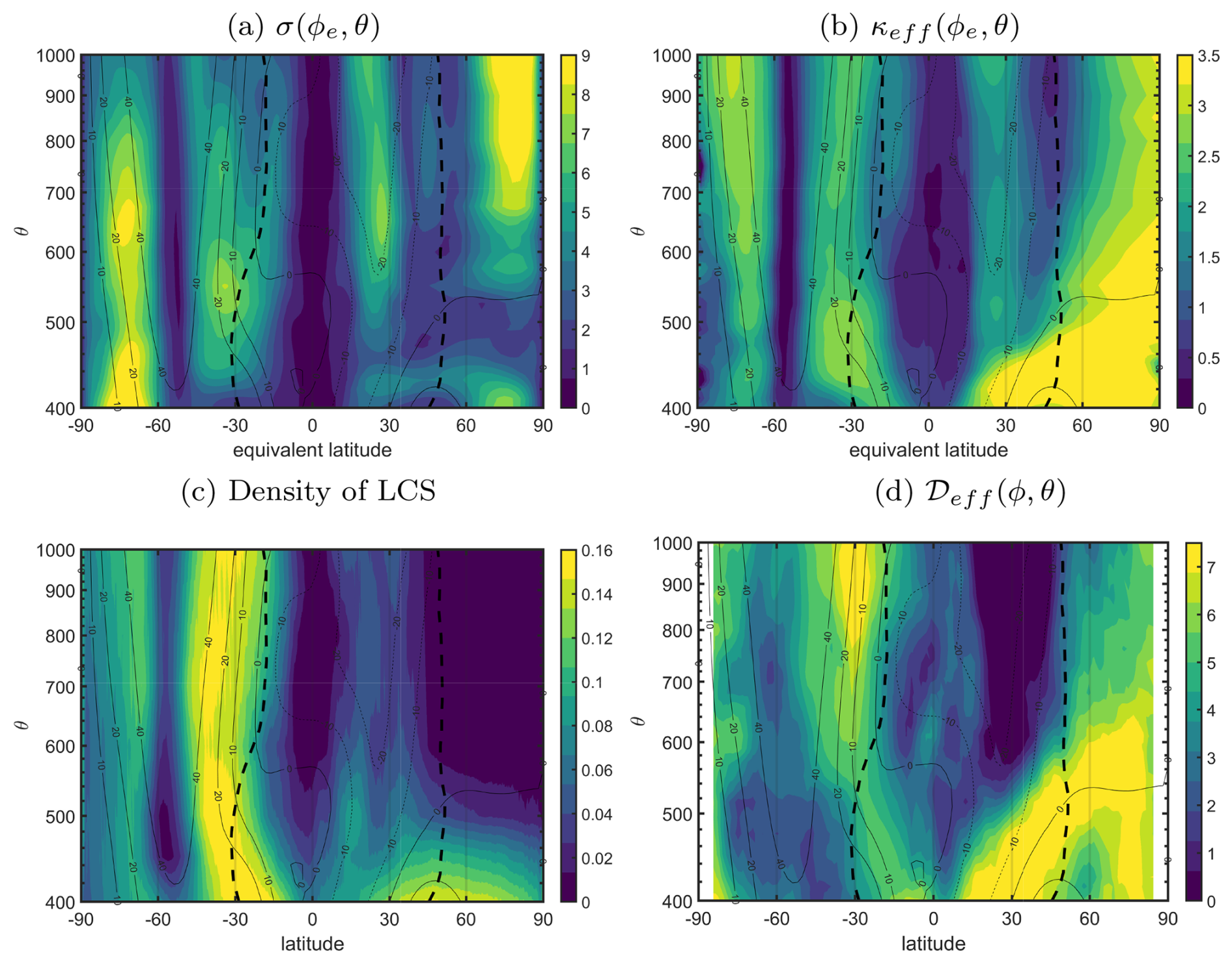
Figure 7 JJA season: (a) standard deviation of the equivalent latitude (in degrees latitude) and (b) effective diffusivity as a function of the equivalent latitude and isentropic levels. (c) Probability density function of the presence of LCS and (d) isentropic eddy diffusivity as a function of the latitude and isentropic levels.

Regarding the Southern Hemisphere, in the places where σ is smaller (60–40° S), we have a better correspondence between κ_eff and LCS density. For higher σ values, the differences between these two metrics are more noticeable, particularly in magnitude. These similarities and differences related to the standard deviation of the equivalent latitude qualitatively support our idea that merely the fact that effective diffusivity is necessarily calculated in ϕ_e coordinates can lead to different results. (We note this is a cautionary example of treating equivalent latitude and latitude as the same quantity.)

3.4 Comparison of LCS density with isentropic eddy diffusivity

The isentropic eddy diffusivity is presented in the bottom row of Fig. 2, and we see that it generally agrees rather well with the overall structures for both effective diffusivity and LCS density. Some noticeable differences are present, including the higher values of isentropic eddy diffusivity in the tropics and the apparent lack of any subtropical mixing in the summer hemisphere. The higher tropical values are consistent with prior results (Abalos et al., 2016b) comparing a tracer-based eddy flux diffusivity to effective diffusivity. The subtropical difference is not as evident in the previous results, however. As effective diffusivity and the LCS density are both lower in the deep tropics, especially as the effective diffusivity should have no effects of time variation of equivalent latitude at these low latitudes, it seems likely that the isentropic eddy diffusivity is providing an overestimate of the mixing. In the lower stratosphere, the LCS density likely overestimates the diffusivity due to the election of constant τ in θ (as mentioned above). However, effective diffusivity is also likely overestimated between 400–500 K in the NH due to the differences between equivalent latitudes in that area (see Fig. 7a). Here, isentropic eddy diffusivity likely gives us the most reliable picture below 500 K, despite the fact that there is better agreement between the LCS density and effective diffusivity.

4 Summary and discussion

In this paper we develop a new diagnostic method to quantify mixing from wind velocities on isentropic surfaces following a Lagrangian approach. The proposed method is based on the definition of Lagrangian coherent structures (Haller and Yuan, 2000), which are special features of fluid flow that are closely linked to the mixing of passive tracers. Using a comprehensive climate model, we present a new and effective approach for quantifying mixing in the atmosphere without relying on equivalent latitude coordinates. This quantitative method establishes a direct relationship between LCS characteristics and mixing/diffusivity measures.

The results obtained using this technique exhibit strong consistency with previous studies, highlighting regions of pronounced mixing near the boundaries of the polar vortices and subtropical edges. Furthermore, areas characterized by limited mixing are identified within the central portion of the vigorous westerlies and within the tropical pipe. Specifically, we have compared the density of LCS to effective diffusivity (Nakamura, 1996) and isentropic eddy diffusivity (Gupta et al., 2023). We emphasize the complementary roles of the three methods used and how they address different aspects of mixing.

We find that the use of the equivalent latitude coordinate likely aliases the seasonal cycle of PV with the seasonal cycle of mixing by examining the variability in equivalent latitude with time. This effect is larger in some regions than others, with little variation present in the tropics and far more in the subtropics and midlatitudes. We therefore caution that using the equivalent latitude coordinate (ϕ_e) may mask certain details of the seasonality. Since equivalent latitude is based on tracer contours, the specific tracer used for the calculation can have an effect on the κ_eff and its variability. The seasonal cycle of PV will be incorporated into the seasonal cycle obtained in κ_eff calculations that use PV to determine equivalent latitude. If a different tracer were used, its seasonal cycle would show up instead, and so the apparent seasonal cycle in effective diffusivity will be dependent on the seasonal cycle of the underlying tracers. In addition, the specific data or model used can make PV less than ideal. For instance, the presence of a high κ_eff band at ϕ_e=20–40° N in JJA in WACCM, which is absent in ERA-Interim reanalysis (see Fig. 1c in Abalos et al., 2016a), raises important questions regarding the reliability of PV-based κ_eff calculations in the summer stratosphere. Previous studies using a diffusion–advection model to evolve a passive tracer (e.g., Abalos et al., 2016a) did not show this feature, suggesting that its appearance in WACCM may be linked to the use of PV or to model-specific biases. Additionally, the occurrence of anomalously high κ_eff values inside the austral polar vortex, exceeding those in the surf zone, further suggests a potential nonphysical behavior in WACCM's PV field. This raises the question of whether PV in WACCM behaves as a well-defined tracer for these calculations. Given that the LCS-based diagnostic, which is derived from the wind field, does not display the high-mixing band in the summer stratosphere, it is reasonable to expect that κ_eff computed using the same winds would not exhibit it either. This supports the notion that the discrepancies may originate from the PV field rather than from intrinsic limitations of the effective diffusivity method.

A definitive way to clarify this issue would be to compute κ_eff in WACCM using a diffusion–advection model with a passive tracer, following the approach of Abalos et al. (2016a), and compare the results with PV-based calculations. However, given the significant computational cost associated with such an approach, it falls beyond the scope of this study. Despite these uncertainties, the fact that the other two mixing diagnostics used in this work do not exhibit similar apparently nonphysical behavior reinforces their robustness. This underscores the importance of employing multiple diagnostics to assess stratospheric mixing. (It also highlights the need for further investigation into the suitability of PV as a tracer in WACCM for κ_eff calculations.) Equivalent latitude is indeed an invaluable tool for characterizing stratospheric dynamics, and it is sensitive to tracer choices and model details.

In summary, our LCS-based metric offers a robust diagnostic tool for comprehending the intricate dynamics of fluid mixing and transport. Furthermore, they can be effectively employed to quantify mixing within the lower and middle stratosphere through the utilization of output from reanalysis products. The LCS-based measures can also provide estimates of the meridional span of adiabatic mixing in the winter/summer midlatitudes and serve as a framework to establish connections between diabatic upwelling and adiabatic mixing, shedding light on the underlying differences between these processes. The LCS density metric has some important limitations, however.

Like isentropic eddy diffusivity, effective diffusivity, and aging by mixing, the LCS-based mixing we examine here cannot be calculated directly from observations. The mixing metrics that can be calculated from observations are based on the TLP model (Ray et al., 2016; Linz et al., 2021), and so they are representing only a mixing coefficient at each latitude rather than a more comprehensive picture of mixing. A good method for calculating spatially resolved diffusivity directly from observations has yet to be developed, as far as the authors are aware.

While the new method discussed offers valuable insights into mixing regions, it does not fully address the challenge of computational cost due to the expense associated with trajectory calculations. By relying solely on wind velocity, it remains particularly useful for preliminary modeling studies, model output, and initial testing phases. We acknowledge its limitations concerning the selection of temporal integration time intervals, especially as the density of LCS depends on the integration time and the temporal scale likely varies with altitude, being different in the stratosphere and troposphere. In the future, we aim to conduct a more in-depth investigation into this topic.

In addition, the LCS density is a measure of mixing more akin to aging by mixing (Garny et al., 2014) than to a true diffusivity, as it is not formulated to have the appropriate units to serve as a coefficient for diffusion. This is something that was addressed for a Lagrangian-structure-based metric using Lyapunov diffusivity (d'Ovidio et al., 2009), but that metric has coefficients that were fit to best match effective diffusivity and is calculated in equivalent latitude. We contend that the qualitative reasoning behind the link between the LCS density and eddy mixing is sound, but a theoretical relationship between the LCS density and diffusivity would enable a more useful diffusion metric. LCSs are typically defined within the context of Hamiltonian (conservative) systems, where the dynamics are purely advective. However, experiments and observations suggest that transient-time diffusion can occur along LCS (e.g., Lehahn et al., 2007; Tang and Walker, 2012). Unlike the limitations of the lack of a ready comparison with data and of the expensive computational needs, this theoretical formulation as a diffusivity is something that could be addressed in future work.

We have introduced an LCS-based mixing metric that is a true Lagrangian metric that nevertheless avoids equivalent latitude. Overall, it agrees quite well with two other metrics for mixing, and we have discussed the disagreements. While we have primarily focused on climatological zonal means for comparative purposes, we acknowledge the need for further testing to validate the new metric comprehensively. Future work will involve additional tests and analyses to better understand its performance and applicability. The applicability of this metric is currently limited because it cannot be calculated directly from observations, because it needs high-temporal-resolution model output, and because it is not directly a diffusivity estimate. There is hope for theoretical progress that would enable a more rigorous definition for a diffusivity based on LCS density, and we also intend to explore some of the vertical dependence of the integration time in the future.