Improved understanding of anthropogenic and biogenic carbonyl sulfide (COS) fluxes in western Europe from long-term continuous mixing ratio measurements

Lack of knowledge still remains on many processes leading to carbonyl sulfide (COS) atmospheric fluxes, either natural, such as the oceanic sources or the vegetation and soil uptakes, or anthropogenic, with emissions from industrial activities and power generation. Moreover, COS atmospheric mixing ratio data are still too sparse to evaluate the estimations of these sources and sinks at the regional scale; in this context, regional estimates are very challenging. This study assesses the anthropogenic emissions and biogenic COS uptakes at the regional scale, in the footprint of a measurement site in western Europe, at a seasonal to diurnal time resolution over half a decade. The continuous time series of COS mixing ratios obtained at the monitoring site of Gif-sur-Yvette (GIF; in the Paris region) from August 2014 to December 2019 are compared to simulations with the Lagrangian model FLEXPART (FLEXible PARTicle), transporting oceanic sources, biogenic land fluxes from the land surface models ORCHIDEE and SiB4 (Simple Biosphere Model), and anthropogenic emissions by two different inventories. At GIF, the seasonal variations in COS mixing ratios are dominated by the contributions of the background and ocean, the weekly to daily variations are driven by the biogenic land contribution and anthropogenic emissions may dominate for short episodes of high concentrations. The anthropogenic emission inventory based on reported industrial emissions and the characteristics of coal power plants in Europe is consistent with the observations. The main limitation of this inventory is the flat temporal variability applied to anthropogenic fluxes due to the lack of information on industrial and power-generation activities in viscose factories and in coal power plants. As a consequence, there are potential mismatches in the simulated plumes emitted from these hot spots. We find that the net ecosystem COS uptake simulated by both ORCHIDEE and SiB4 is underestimated in winter at night, which suggests improvements in the parameterization of the nighttime uptake by plants for COS. In spring, SiB4 simulates persistent nighttime uptake by vegetation, which is different than ORCHIDEE, which leads to more realistic simulations with SiB4 than with ORCHIDEE. In summer, both models represent fluxes sufficiently well, with better agreement from ORCHIDEE in terms of magnitudes.

1 Introduction

Carbonyl sulfide (COS) is absorbed along with CO₂ by plants during photosynthesis. But COS, different than CO₂, is almost not emitted during respiration-like processes (Protoschill-Krebs et al., 1996; Montzka et al., 2007; Sandoval-Soto et al., 2005; Ma et al., 2021; Kuai et al., 2015; Campbell et al., 2017; Kettle et al., 2002; Suntharalingam et al., 2008). This has led to suggestions that COS could be used as a tracer for quantifying and/or reducing uncertainties in CO₂ fluxes due to photosynthesis (e.g., Whelan et al., 2018; Launois et al., 2015; Hilton et al., 2017, 2015).

The methodology called atmospheric inversion consists in assimilating mixing ratio data into a statistical framework (called Bayesian because it is based on Bayes' theorem), making use of some prior knowledge of sources and sinks and of a chemistry-transport model (CTM) to link fluxes (either emissions to the atmosphere or uptake) to atmospheric mixing ratios, in order to estimate optimized fluxes. The optimized fluxes are statistically consistent with all the information provided by the prior knowledge of sources and sinks and by the measured atmospheric mixing ratios. The minimum requirements for atmospheric inversion to yield useful insights are therefore not only (i) that the CTM resolution, various inputs (such as meteorological fields, flux maps), and physical and chemical parameterizations are relevant to the targeted spatio-temporal scale so that the link between fluxes and atmospheric mixing ratios does not entail large or poorly characterized uncertainties but also (ii) that the uncertainties in the prior knowledge of sources and sinks are well characterized so that the corrections applied to obtain optimized fluxes are physically meaningful. On top of these general requirements, when using COS mixing ratio data to get information on CO₂ uptake during photosynthesis, the atmospheric inversion must be provided with information that makes it possible to disentangle the influence of the biogenic sink of COS from the influence of anthropogenic and other biogenic fluxes on the measured COS mixing ratios. This can be done by providing fluxes of COS to the CTM which are well known, i.e., with small and well-characterized uncertainties. A strong limitation to today's potential use of COS for gaining insight into CO₂ photosynthesis fluxes is that COS sources and sinks are not very well known, with only a few estimations available for the various categories (Whelan et al., 2018; Remaud et al., 2023a), which can be summarized as follows (see also Table 1).

• The natural oceanic source is due to both direct COS emissions and indirect emissions via dimethyl sulfide (DMS) and carbon disulfide (CS₂) (Mihalopoulos et al., 1992). Note that freshwaters also contribute to COS emissions (Du et al., 2017). In the atmosphere, CS₂ is oxidized into COS in about 10 d (Bandy et al., 1981; Khalil and Rasmussen, 1984; Chin and Davis, 1993; Stickel et al., 1993). Total direct and indirect oceanic emissions are estimated at 265 ± 210 Gg S yr⁻¹ by Lennartz et al. (2017) (cited in Whelan et al., 2018) and Lennartz et al. (2021).

• Anthropogenic sources of COS are restricted to particular industries, once again in contrast to CO₂. These anthropogenic sources are due to industries which emit either COS or CS₂. The main source of anthropogenic COS is the oxidation of CS₂ emitted by the viscose industry, which includes factories producing viscose as their final product (hereafter named the viscose-producing industry) or as the byproduct of their main process for producing, e.g., sponges or cellophane (Chen, 2015; U.S. Environmental Protection Agency Office of Water, 2011) (hereafter named viscose processors). Other sources are smaller and emit both COS and CS₂: they not only are in the sector of energy production with coal use in power plants but also include the combustion of oil and bio-fuels (Attar, 1978), pulp mills due to the kraft process (Brownlee et al., 1995; Cheremisinoff and Rosenfeld, 2010), industries using aluminum oxide electrolysis to produce aluminum (Harnisch et al., 1995), and the producers of pigments with carbon black used for tires or the food industry and the widely used white titanium dioxide. For the whole world in the year 2012, the inventory by Zumkehr et al. (2018) gives a total of 400 ± 180 Gg S yr⁻¹ for all anthropogenic emissions (used in the budget elaborated by Whelan et al., 2018).

• Besides the anthropogenic combustion of bio-fuels, biomass burning from either natural (e.g., wildfires due to lightning) or human-caused (e.g., agricultural practices) open fires is also a source of COS, estimated at an average of 60 ± 37 Gg S yr⁻¹ by Stinecipher et al. (2019).

• Soils can also be sources of COS under specific conditions such as high temperature and incoming radiation, related to abiotic production processes (Whelan and Rhew, 2015; Whelan et al., 2016, 2018; Kitz et al., 2017, 2020). The anoxic soil contribution has recently been estimated at 96 Gg S yr⁻¹ with the ORCHIDEE process model (Abadie et al., 2022b; see also details on ORCHIDEE in Sect. 2.2.2).

• The main biogenic sink is due to the uptake of COS by vegetation (Whelan et al., 2018): COS is irreversibly consumed by the carbonic anhydrase enzyme in leaves (DiMario et al., 2016). Soils can also absorb COS due to soil microorganisms that also contain the carbonic anhydrase enzyme (Masaki et al., 2021). The order of magnitude obtained for the uptake by vegetation is −530 Gg S yr⁻¹ with the ORCHIDEE process model (see details on ORCHIDEE in Sect. 2.2.2), which can be compared to, for example, −664 Gg S yr⁻¹ with the Simple Biosphere Model (SiB4; Kooijmans et al., 2021a). The oxic soils can both produce and consume COS, but they are a net sink, estimated recently at −126 Gg S yr⁻¹ with the ORCHIDEE process model (Abadie et al., 2022b). The net soil sink (taking into account the source due to anoxic soils and the net sink due to oxic soils) of COS is therefore estimated at −30 Gg S yr⁻¹ by Abadie et al. (2022b), which can be compared to, e.g., −89 Gg S yr⁻¹ according to SiB4 (Kooijmans et al., 2021a).

• The atmospheric sink of COS is due to its oxidation by OH radicals and its photolysis in the stratosphere (estimated at −130 to −80 and −50 ± 15 Gg S yr⁻¹, respectively, by Whelan et al., 2018).

Reducing the uncertainties in the estimates of all these sources and sinks at the global scale at as fine temporal and spatial resolutions as would be required to bring information on CO₂ fluxes due to photosynthesis does not seem easy to accomplish in the next few years. The first challenge is the lack of knowledge still remaining regarding many processes which lead to COS or CS₂ emissions in the atmosphere. For example, Remaud et al. (2023a) and Ma et al. (2023, 2021) conclude that a source may be missing in the tropics (probably from the ocean) and that the uptake of COS by vegetation at high northern latitudes is too small. Some natural processes emitting COS in the atmosphere are still only suspected, for example in plants used in agriculture (Belviso et al., 2022a; Maseyk et al., 2014; Bloem et al., 2012). The second difficulty is the lack of data on COS atmospheric mixing ratios (Montzka et al., 2007), which could be used in CTMs to evaluate the available estimations of sources and sinks at the regional scale, although the National Oceanic and Atmospheric Administration (NOAA) provides atmospheric mixing ratios of COS at several stations, which are useful at the global scale. Still, NOAA data are based on monthly or at best biweekly flask samples, limiting our ability to use them to constrain fluxes at scales smaller than the global to continental scales. Observations with higher frequencies are very sparse globally (Belviso et al., 2020; Kamezaki et al., 2023; Zanchetta et al., 2023; Kooijmans et al., 2016; Commane et al., 2015) and were not yet used for long-term systematic assessment of regional COS fluxes.

To begin to tackle the issue, Belviso et al. (2020) have made use of one of the few continuous time series of COS atmospheric mixing ratios available in the Paris region to assess the budget of COS in this area at the seasonal scale and during pollution peaks. Even though the area is almost always a COS sink, local biogenic emission episodes appear in summer and anthropogenic emissions from the Benelux, eastern France and Germany are occasionally transported so as to influence the area in winter. Belviso et al. (2022b) then tried to use the information brought by the same COS time series of mixing ratios to learn more about the anthropogenic emissions in the footprint of the station, which covers part of western Europe (including Benelux, eastern France and Germany) and part of the Atlantic. Anthropogenic emissions in the footprint of Gif-sur-Yvette (GIF) were proven to be overestimated when analyzing specific events selected in the relatively long continuous time series available. Nevertheless, further characterization was not possible at the time of the study. Following these results, Belviso et al. (2023) used a semi-quantitative approach to assess the gridded inventory of direct and indirect anthropogenic emissions of COS by Zumkehr et al. (2018) in France. The main conclusion of this work is that COS emissions in France are overestimated in this inventory by 1 order of magnitude and another way of mapping these emissions is required.

Therefore, this study aims at quantitatively assessing the anthropogenic and biogenic COS fluxes at the regional scale. It demonstrates that a setup based on one measurement site in western Europe, which provides data for over half a decade, makes it possible to

• quantitatively assess the discrepancies in Zumkehr's anthropogenic emission inventory in the footprint of the measurement site

• evaluate a new inventory based on the industrial emission declaration in the European Union

• study the seasonal and diurnal cycles of biogenic fluxes, based on the ORCHIDEE and SiB4 process-based land surface models, and point to strengths and weaknesses in these two models.

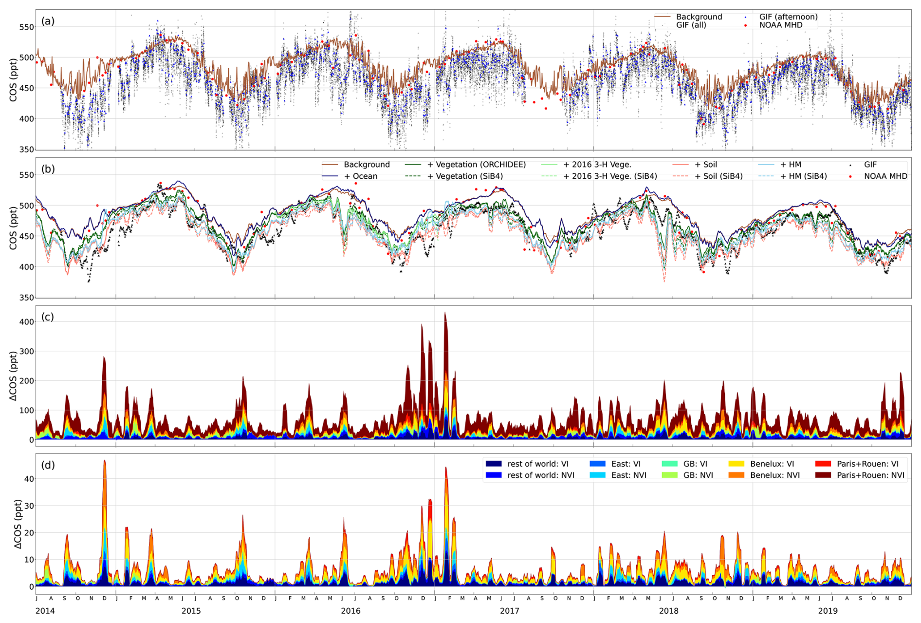
Figure 1 Time series of observed and simulated atmospheric mixing ratios of COS. (a) Hourly COS observations at GIF, with afternoon (12:00–18:00 UTC) averages superimposed, and flask measurements at Mace Head (MHD) and the simulated background described in Sect. 2.3. Remark: the limits set on the y axis do not show ≈ 50 extremely low values and ≈ 190 extremely high values of hourly COS observations. (b) The 10 d rolling mean of GIF afternoon observations, with cumulative simulated contributions from the background, ocean sources, and biogenic land fluxes (see Sect. 2.3 for details; 2016 3-H Vege.: 3-hourly vegetation uptake as available for 2016). (c) The 10 d rolling mean of simulated anthropogenic contributions to COS mixing ratios by region (shown in Fig. 2) and sector according to Zumkehr's inventory (see Sect. 2.2.3; VI: viscose industry, NVI: non-viscose-related industry). (d) The 10 d rolling mean of simulated contributions by region (shown in Fig. 2) and sector according to our homemade inventory (HM; see Sect. 2.2.3, Fig. 2). Remark: afternoon data are shown here because the model is assumed to better represent the vertical mixing in the afternoon so that the comparison to measurements highlights the discrepancies in fluxes compared to the model's errors.

For this, we use the continuous time series of COS mixing ratios measured in the Paris region from summer 2014 to the end of the year 2019, as described in Sect. 2.1. We compare them to the concentrations simulated from marine, biogenic and anthropogenic fluxes in the area of interest (detailed in Sect. 2.2) combined with the contribution due to the rest of the world (Sect. 2.1) using the modeling tool described in Sect. 2.3. After an assessment of the general performance of the model (Sect. 3.1), we are able to quantitatively evaluate the anthropogenic sources from western Europe as estimated by Zumkehr et al. (2018) (hereafter referred to as Zumkehr's inventory) and by our more targeted inventory (Sect. 2.2.3), confirming discrepancies from Belviso et al. (2023) in Zumkehr's inventory not only in France in particular but also in western Europe in general. Contrary to Belviso et al. (2023), the present study goes one step further by quantitatively assessing discrepancies in Zumkehr's inventory and by proposing a new inventory based on the industrial emission declaration in the European Union. Having more reliable anthropogenic emissions, we can inquire into biogenic emissions, which is one of the main original purposes of studying COS. We study the seasonal and diurnal cycles of biogenic fluxes, based on the ORCHIDEE and SiB4 process-based land surface models (Sect. 3.3); this allows us to point to strengths and weaknesses in the two models.

2 Data and methods

2.1 Measurements and setup of background mixing ratios

The measurements used in this study constitute a quasi-continuous time series of COS atmospheric mixing ratios obtained at the monitoring site of Gif-sur-Yvette (GIF) located in the Paris region at 48.7109° N, 2.1476° E at 163 $\mathrm{m}\mathrm{a}.\mathrm{s}.\mathrm{l}.$ with an inlet height of 7 $\mathrm{m}\mathrm{a}.\mathrm{g}.\mathrm{l}.$ A commercial gas chromatograph (Varian 3800) coupled with a cryogenic preconcentrator (ENTECH P7100) for sample preparation and a mass spectrometer detector (Varian Saturn 2200) for COS detection was used to analyze this gas, as described by Belviso et al. (2013, 2016, 2020). Calibration and drift correction is done every 3 weeks using a calibration gas containing 1.013 ppm of COS in helium, with the occasional calibration using a standard of compressed air with 573 ppt of COS and another standard traceable to the NOAA ESRL standard of 448.6 ppt. Calibrations led to a repeatability of 1 % and a precision of 0.2 %.

The GIF time series of hourly data spanning August 2014 to December 2021 is available in Belviso et al. (2022b). In this study, we only make use of the time series from August 2014 to December 2019 (Figs. 1 and A1 to A6), which covers the period of availability of inputs required for simulations, in particular global concentration fields used to compute the background signal (see Sect. 2.1 and 2.3).

The time series of flask measurements sampled by the National Oceanic and Atmospheric Administration (NOAA) network at Mace Head (MHD) in Ireland at 53.3° N, 9.9° W at 42 $\mathrm{m}\mathrm{a}.\mathrm{s}.\mathrm{l}.$ (described in Montzka et al., 2007, with one to five pairs of flasks per month, collected mostly between 08:00 and 17:00 UTC) is also shown in Fig. 1 to illustrate the so-called “background”, i.e., the overall contribution of all the sources and sinks which are not in our area of interest. In our study, which focuses on western Europe and more particularly on the footprint of GIF, the mixing ratios at MHD are representative of the background when the air masses are advected from the west, which is a frequent meteorological configuration (Belviso et al., 2020).

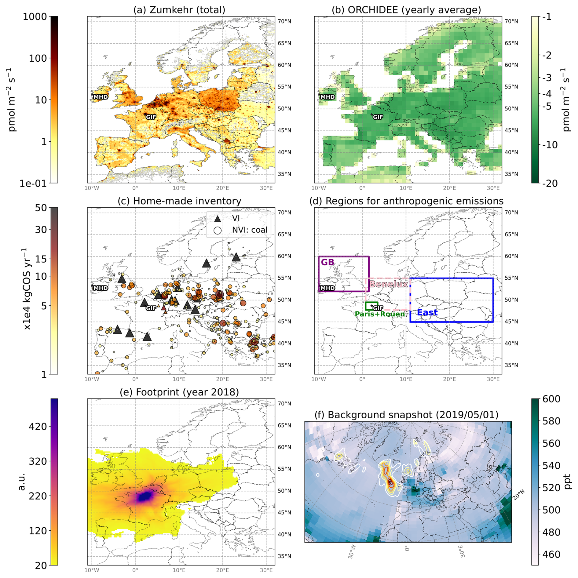
Figure 2 Maps of input data sets used in our study. (a) Zumkehr's yearly, i.e., 2012, total emissions; (b) 2019 yearly average biogenic land fluxes from the ORCHIDEE model; (c) emission points from viscose and coal industries as defined using our methodology (see Sect. 2.2.3 for details; here the year 2019 is shown for illustration); (d) regions of interest for anthropogenic emissions; (e) illustration of the footprint summed up over the year 2018; (f) snapshot of background concentration fields. Contours highlight the computed sensitivity to the background 10 d before observation at GIF (see Sect. 2.3 for details). Remark: units for area (gridded) emissions are pmol m⁻², whereas emissions by point sources are in mass units; footprints are shown in arbitrary units (a.u.).

The contribution of the background to the simulated mixing ratios is computed using 3D fields at the global scale (see details in Sect. 2.3). The COS mixing ratio fields used here are obtained from Remaud et al. (2022), at a horizontal resolution of 3.75° in longitude and 1.875° in latitude for 39 pressure levels at a 3-hourly time resolution (illustration in Fig. 2). These global atmospheric inversions were designed to assimilate data from the background NOAA observation sites, such as MHD.

2.2 Fluxes

In the following, “emission” denotes fluxes which are sources as seen from the atmosphere and “uptake” denotes fluxes which are sinks as seen from the atmosphere; “flux” is used for (ensembles of) processes which can be either sources or sinks.

Lennartz et al. (2017, 2021)Remaud et al. (2022)Zumkehr et al. (2018)Stinecipher et al. (2019)Abadie et al. (2022a)Abadie et al. (2022a)Abadie et al. (2022a)Kooijmans et al. (2021a)Kooijmans et al. (2021a)Whelan et al. (2018)Whelan et al. (2018)

Table 1 COS sources and sinks: global estimates available at the time of this study, from Whelan et al. (2018) and Remaud et al. (2023a).

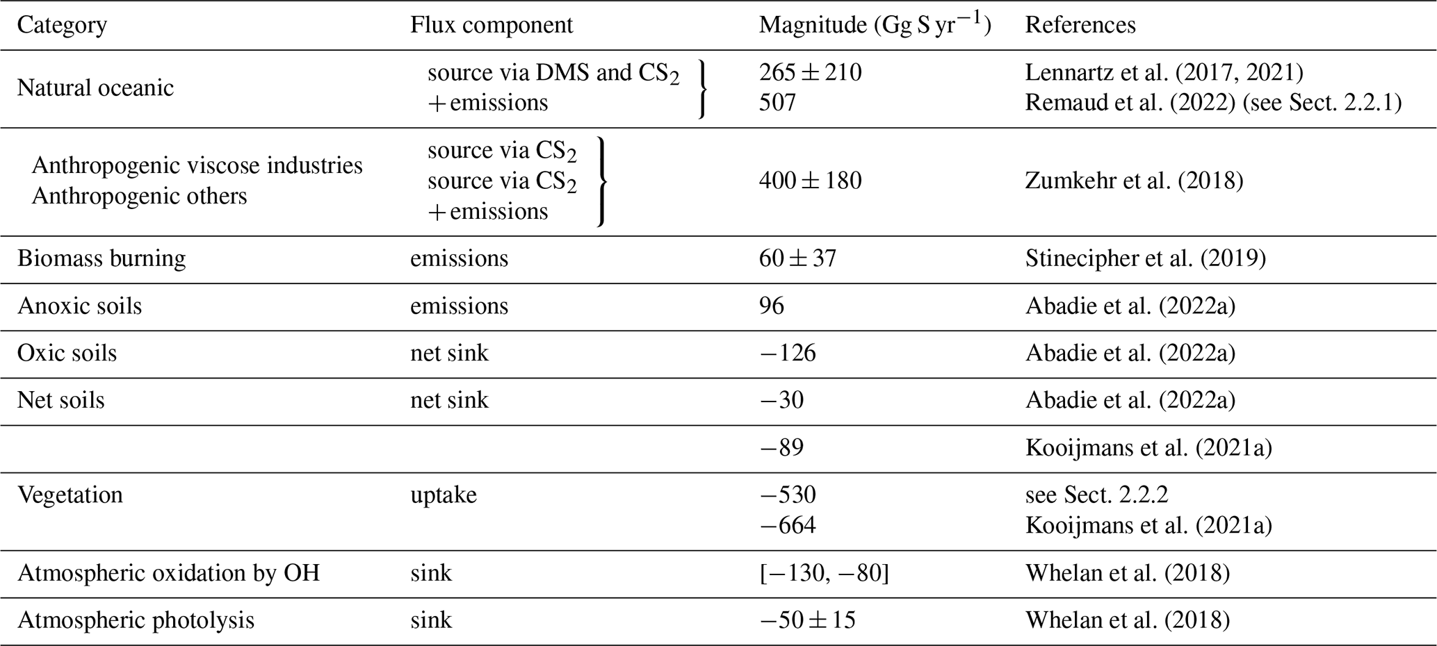
Our simulations, detailed in Sect. 2.3, take into account COS fluxes in the area of interest as provided by the data sets described here and listed in Table 1. The contributions from biomass burning emissions and the atmospheric sink are neglected in this study, as well as the emissions from anoxic soils. They play a significant role at the global scale for long-term studies (e.g., Ma et al., 2023) but are negligible compared to ocean emissions (see Sect. 2.2.1), biogenic fluxes (see Sect. 2.2.2) and anthropogenic emissions (see Sect. 2.2.3).

2.2.1 Ocean emissions

The ocean data set designed by Lennartz et al. (2021, 2017) includes direct emissions of COS and indirect emissions of COS via CS₂ and dimethylsulfide (DMS) emissions at a monthly resolution and at a 1° × 1° horizontal resolution, respectively. Anthropogenic DMS emissions also exist. However, Sarwar et al. (2023) and von Hobe et al. (2023) have shown that their impact (through oxidation) on simulated COS concentrations is negligible.

The emissions of the three species have been computed using coarse-resolution box models calibrated with shipborne measurements made in different parts of the globe and result in a data-driven data set for COS oceanic emissions. This ocean data set has been optimized by Remaud et al. (2022) by assimilating NOAA flask data into the model LMDZ. This optimized data set has been compared to others by Ma et al. (2023) (therein called OPT-LMDZ) and gives very similar results to other data sets when evaluated with independent atmospheric data at the global scale. Our ocean fluxes give total (direct + indirect) emissions of COS of 507 Gg S yr⁻¹ on average over 2014–2019 and 4 Gg S yr⁻¹ in our domain of interest.

2.2.2 Biogenic land fluxes

In this study, biogenic land fluxes refer to vegetation uptake and soil exchanges. We compare simulations based on the ORCHIDEE (Krinner et al., 2005) and SiB4 (Haynes et al., 2019b, a) land surface models.

In ORCHIDEE and SiB4, a mechanistic representation of vegetation COS uptake has been implemented following Berry et al. (2013), and soil COS exchanges are computed based on the model from Ogée et al. (2016), representing both COS uptake and emission by soils. The representation of biogenic COS fluxes in SiB4 is described in detail in Kooijmans et al. (2021b), while the vegetation and soil COS models in ORCHIDEE are presented in Maignan et al. (2021) and Abadie et al. (2022b), respectively.

Biogenic land fluxes are computed with a horizontal resolution of 1° × 1° at a monthly time step (illustrated in Fig. 2), thus losing any temporal variability at the synoptic scale. The data set used here estimates the average uptakes of COS over 2014–2019 at 22.6 Gg S yr⁻¹ (29.8 Gg S yr⁻¹) by the vegetation according to ORCHIDEE (SiB4) and 12.9 Gg S yr⁻¹ by the soil in our domain of interest. In particular, real-life biogenic fluxes exhibit a significant diurnal cycle (whereas modeled fluxes are constant). Indeed, vegetation COS uptake is regulated by stomatal conductance. There is a residual uptake during nighttime due to incomplete stomatal closure and a stronger uptake during daytime when stomatal conductance increases. We assess the sensitivity of our simulations to daily varying biogenic fluxes using 3-hourly vegetation uptake as simulated by ORCHIDEE and SiB4 for the year 2016. The different performance of the models with monthly and 3-hourly fluxes is evaluated in Sect. 3.3.

2.2.3 Anthropogenic emissions

Two different COS anthropogenic inventories are used in this study. The inventory by Zumkehr et al. (2018) accounts a total of 62.1 Gg S yr⁻¹ in the domain of interest, compared to our more realistic inventory, with a total of 11.2 Gg S yr⁻¹.

Main characteristics of Zumkehr's inventory

The inventory by Zumkehr et al. (2018) accounts for the sectors emitting the most COS and CS₂ at the country level and provides yearly emissions from 1980 to 2012. Here, the values for the year 2012, as the most recent available, have been used. In our domain of interest, they amount to a total of 62.1 Gg S yr⁻¹, among which 20.5 Gg S yr⁻¹ is for the viscose industry, 14.5 Gg S yr⁻¹ is for coal use, 23.6 Gg S yr⁻¹ is for the pigments and 2.8 Gg S yr⁻¹ is for aluminum production, with minor contributions from industrial solvents and the paper industry. The sub-country distribution is done according to secondary proxies, such as energy industry activity or industrial CO₂ emissions. This proxy-based distribution proved effective in the US but can be misleading in some European countries. For example, in France, only one power plant is fueled by coal and only a very few viscose sites are still active, not necessarily near the biggest cities in the country. Opposite to this, Zumkehr's methodology leads to a distribution of national emissions around the main urban areas, decorrelated to real emissions. As shown in Fig. 2 and Fig. 1c of Belviso et al. (2023), such a hot spot appears in the Paris region, with its center located close (about 20 km) to the northeast of GIF.

In the following, the sectors provided in Zumkehr's inventory (Table 1 of Zumkehr et al., 2018) are grouped as emissions for the viscose industry (abbreviated as VI), which include the sectors pulp and paper, rayon staple and rayon yarn, and the non-viscose-related industry (abbreviated as NVI), which include the sectors agricultural chemicals, aluminum smelting, carbon black, industrial coal, residential coal, industrial solvents, titanium dioxide (TiO₂) and tires. Maps and bar plots for selected European countries are available in the main text and supplementary material of Belviso et al. (2023).

Homemade inventory

To overcome the caveats of Zumkehr's inventory in western Europe, we designed our own inventory following the conclusions of Belviso et al. (2023) and based on the following.

• An explicit declaration of CS₂ emissions from the viscose industry (including rayon yarn and staple and other products such as cellulosic casings) with a comprehensive list of plants in Europe (abbreviated as VI and comparable to the VI emissions in Zumkehr's inventory) for the year 2018 (available at the time of the study) are used (see details in Tables 2 and 3 of Belviso et al., 2023). The total emissions in our domain of interest are ≈ 4.7 Gg S yr⁻¹ in 2018. How our simulations take into account the oxidation of CS₂ into COS is described in Sect. 2.3.

• For coal, CO₂ emissions for all coal power plants in Europe (from the Global Energy Monitor's Global Coal Plant Tracker) were used to estimate COS emissions for each year based on a unique emission factor (abbreviated as NVI and comparable to the NVI coal-related emissions in Zumkehr's inventory). We used a value of 5.7 × 10⁻⁶ molecules of COS emitted for each molecule of CO₂ during coal combustion. The average emissions over 2014–2019 are ≈ 6.5 Gg S yr⁻¹ in our domain of interest.

Due to lack of data, we did not apply any temporal profiles to viscose and coal emissions, even though they are expected to strongly vary over the year, even from one week to the next. For viscose, we applied no inter-annual variability and keep emissions stable based on the year 2018. For coal emissions, inter-annual variability is based on yearly CO₂ emission values. Compared to Zumkehr's inventory, ours (Fig. 2) displays only a few hot spots of emissions in France: four viscose industry sites with big factories and four coal-burning power plants. The one closest to GIF (large black triangle in northern France in Fig. 2c) is in the city of Beauvais, which lies about 85 km to the north of GIF, i.e., further than the Paris region.

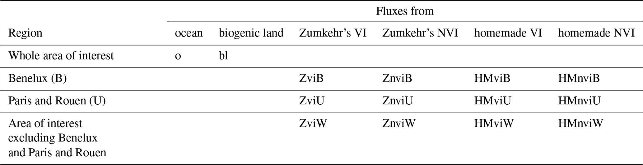
Table 2 FLEXPART simulations per region (shown in Fig. 2) and sector. Each cell: a group of letters indicate that the simulation is run; the same IDs are used for each violin plot in Fig. 3. Z: Zumkehr's inventory, HM: homemade inventory (this study), VI (or vi): viscose industry, NVI (or nvi): non-viscose-related industry (actually coal-related only in HM; see Sect. 2.2.3), U: Paris and Rouen (an urban and industrial area), B: Benelux, W: whole area excluding B and U.

2.3 Simulations of concentrations

The modeled COS mixing ratios were obtained using the Lagrangian atmospheric transport model FLEXPART (FLEXible PARTicle) version 10.3 (Stohl et al., 2005; Pisso et al., 2019). The FLEXPART model is driven by meteorological data from the European Centre for Medium-Range Weather Forecast (ECMWF) ERA5 reanalysis (Hersbach et al., 2020) with 3-hourly intervals and 60 vertical layers, retrieved using the FLEX-extract toolbox (Tipka et al., 2020). The performance of ERA5-provided boundary layer height and wind direction is very good (e.g., Molina et al., 2021). In our case, meteorological data are provided to FLEXPART at a 1° horizontal resolution. For the whole duration of the observation period, 2000 virtual particles are released every 6 h and followed backward in time for 10 d. The multiple FLEXPART simulations are driven by the GUI (graphical user interface) toolbox designed by Berchet et al. (2023). FLEXPART and ERA5 meteorological data are well-recognized tools in the atmospheric community, with the combination of the two being widely used in the atmospheric inversion community (Pisso et al., 2019; Bakels et al., 2024). The choices made for FLEXPART's configuration (number of particles released, frequency of releases, resolution) are consistent with the setups used for the atmospheric inversion fluxes (e.g., Bergamaschi et al., 2022; Thompson et al., 2021).

We assume a conversion of CS₂ to COS with a maximum of 87 % molar conversion rate, as used by Zumkehr et al. (2018). The kinetics of the conversion is approximated by prescribing a half-life of 3 d to CS₂ in the atmosphere. The amount of COS created from a CS₂ source along the transport path of the air mass is then given as 0.87 × $(\mathrm{1}-e^{-\frac{t}{\frac{\mathit{\tau }}{\text{ln}\mathrm{2}}}})$ with τ = 3 d. Note that a lifetime of 1.5 d has also been tested (not shown), with almost no changes in the conclusions of this study.

So-called source-sensitivity (or footprint) maps (Seibert and Frank, 2004) are computed for every release date by counting the number of particles transported above a certain point below a threshold of 500 $\mathrm{m}\mathrm{a}.\mathrm{g}.\mathrm{l}.$ The source contribution by process type is inferred by convolving source-sensitivity maps with flux maps from the ocean emissions, the biogenic fluxes and one of the two anthropogenic emission inventories (see Sect. 2.2.1–2.2.3). One FLEXPART simulation is run for each process or sector and region of interest (see Fig. 2) so that the simulations (Table 2) can be combined to include or exclude particular sectors and/or particular regions when building the footprint maps.

The background mixing ratios (Fig. 2f) are calculated by combining the 3D source-sensitivity fields (e.g., Thompson and Stohl, 2014; Pisso et al., 2019) at the end of the backward trajectories with the available COS concentration field (see Sect. 2.1). The background thus obtained represents the average of the mixing ratios in the grid cells where each particle trajectory terminated 10 d before the observation. For instance, as illustrated in Fig. 2f, for the given date, GIF observations are sensitive to background mostly in the northwestern Atlantic (higher sensitivity for dark-red contours). The computation of COS contributions from surface fluxes and the background was carried out using the Community Inversion Framework (CIF; Berchet et al., 2021).

3 Results and discussion

3.1 General patterns of simulated and measured COS concentrations at GIF

At GIF, the seasonal variations in COS mixing ratios are dominated by the contributions of the background and ocean, i.e., by large-scale fluxes; the variations at shorter timescales (weeks or days) are driven by the biogenic land contribution (Belviso et al., 2023). Finally, depending on the wind speed and direction, anthropogenic emissions may dominate for short episodes of high concentrations (see Sect. 3.3.2, “Selected winter episodes”, in Belviso et al., 2023). The contributions to COS mixing ratios at GIF due to the ocean, the biogenic land fluxes and the anthropogenic emissions are shown in Fig. B1.

In the following, we use the afternoon (12:00–18:00 UTC) daily averages of measured and simulated mixing ratios because the model is assumed to better represent the vertical mixing in the afternoon so that the comparison to measurements highlights the discrepancies in fluxes compared to the model's errors. More detailed results for the whole day or nighttime and per season are shown in Table C1.

Table 3 Statistical indicators of the performance of the model compared to the measurements at GIF for each contribution, based on the daily afternoon (12:00–18:00 UTC) means of simulated and measured mixing ratios; indicators are computed either over the whole period, i.e., August 2014–December 2019 (see Sect. 2.1), or only over the year 2016 for comparison with the available contribution by the 3-hourly varying vegetation. Bias: mean difference model minus measurement, RMS: root mean square model minus measurements, correlation: Pearson's correlation coefficient between model and measurement time series. HM indicates emissions from our homemade inventory (see Sect. 2.2.3).

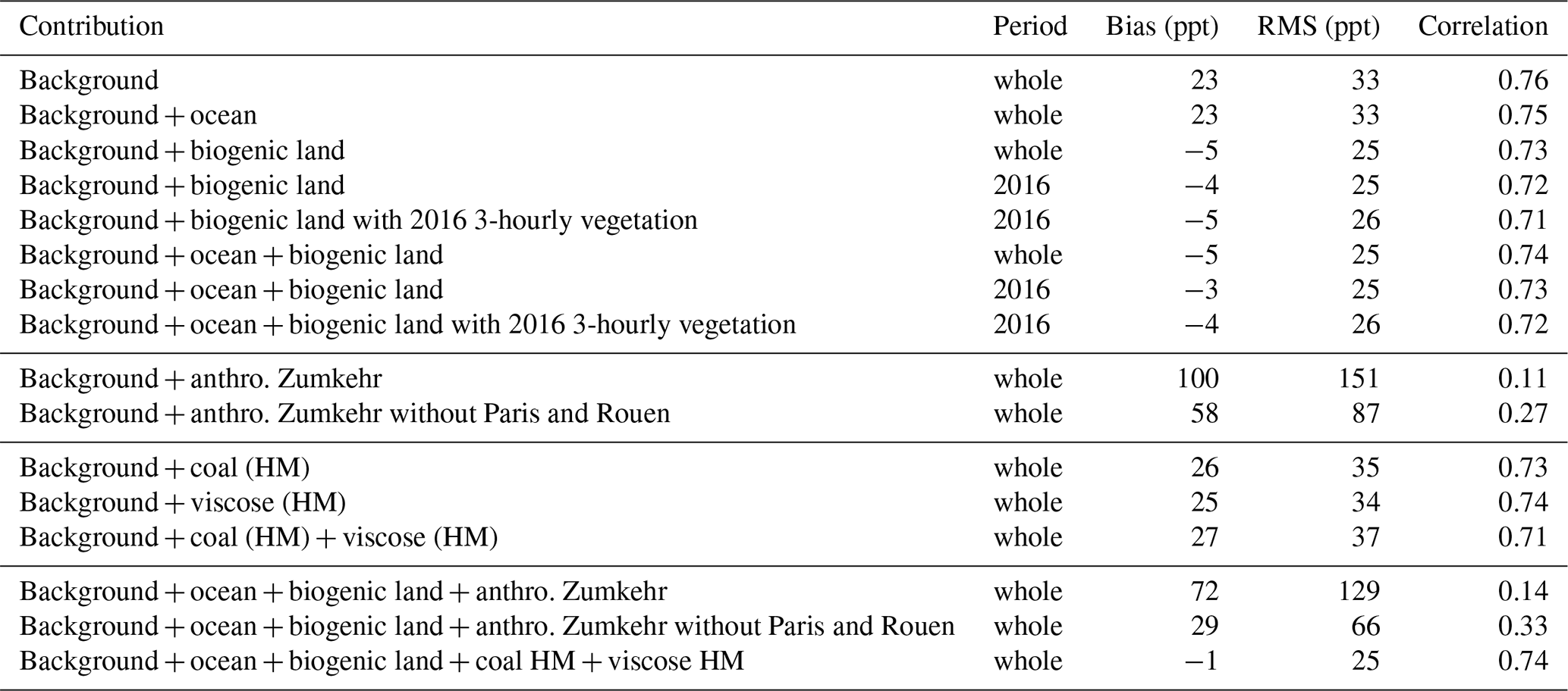
By design, the background contribution (Sect. 2.1) fits the main monthly variations as measured at a background station such as MHD (Fig. 1a and b). Its contribution at GIF ensures a good simulation of the variability (Table 3, Pearson's correlation of ≥ 0.75) and a baseline mean error of ≤ 35 ppt over the whole period of interest. As expected, adding the natural emissions from the ocean (Sect. 2.2.1) and the biogenic land fluxes (Sect. 2.2.2) reduces the bias (by almost 15 ppt as an absolute value) and the mean error is decreased by more than 0 %.

As mentioned in Sect. 2.2.2, we assess the impact of using temporally resolved biogenic fluxes on our simulations. Making use of vegetation uptake with a 3-hourly time resolution (only during the year 2016; see Sect. 2.2.2) does not improve the statistical fit of the model to the observations: the three statistical indicators are almost unchanged (Table 3, period of 2016). The variability is not better reproduced when adding the natural emissions from the ocean and the biogenic land emissions from the soils and the vegetation to the background (correlations of ≤ 0.75 in all cases). This may be due to the monthly resolution of the ocean emissions (Sect. 2.2.1) being too coarse compared to the variability in the transport and to an issue with the variability in the vegetation uptake or the soil exchanges, probably at the seasonal scale, which is assessed in Sect. 3.3.

The limited impact and even degradation of performance when using the diurnal cycle of biogenic flux suggest an issue in their representation in ORCHIDEE, potentially in the residual ecosystem (vegetation and soil) COS flux simulated at night.

The contributions of the anthropogenic emissions by Zumkehr degrade all three indicators of the fit to the measured concentrations at GIF: the bias and mean error are very high (both ≥ 100 ppt), and the variability is not reproduced anymore. The regional anthropogenic emissions located in the Paris and Rouen area explain the major part of the discrepancies between the simulation and the measurements (Table 3). According to Zumkehr's inventory, COS emissions in Île-de-France, i.e., the Paris region itself, are mostly (≈ 62 %) due to the viscose industry, which is not consistent with the lack of any such factory declaring emissions in this region. The small (< 1 %) contribution by the coal-using industry is not consistent with the last coal power plant in the area being closed in 2012. Due to the same type of incomplete information or lack of a relevant proxy, the overall European COS emissions in Zumkehr's inventory may be overestimated, as suggested by the very high contributions (more than 100 ppt) due to anthropogenic emissions alone simulated at GIF (Fig. 1c).

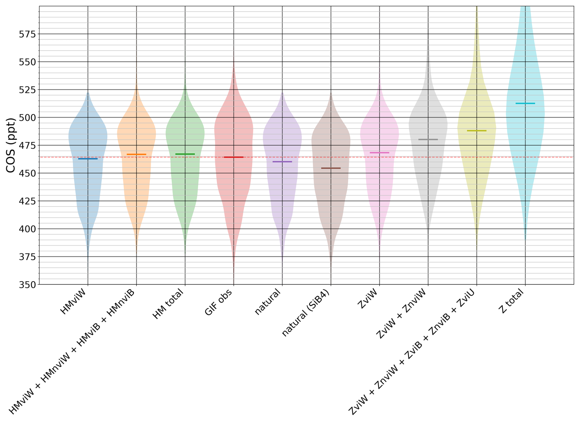
Figure 3 Violin plots of COS mixing ratios at GIF (solid horizontal lines show the medians) for observations (GIF obs) and various simulations taking into account different sets of contributions. See Table 2 for the available simulations per region and per sector; natural: background + o + bl, Z total: natural + ZviW + ZnviW + ZviB + ZnviB + ZviU + ZnviU, HM total: natural + HMviW + HMnviW + HMviB + HMnviB + HMviU + HMnviU.

The contribution of the anthropogenic emissions from our homemade inventory increases the bias and mean error compared to the contributions of the background and natural fluxes only (Table 3). The maximum simulated contributions are between 40 and 50 ppt for some months (Fig. 1c and d), i.e., 10 times smaller than with Zumkehr's inventory. Therefore, the bias and mean error computed over the whole period using our inventory remain more than 2 times smaller than with Zumkehr's inventory without the emissions of the Paris and Rouen area. This order of magnitude is more consistent with the expected anthropogenic contribution required to match the measured concentrations above the background at GIF. Overall statistics are very similar when using only viscose or coal or both. Further investigation is needed to narrow the range of anthropogenic fluxes in Europe. However, as anthropogenic contributions are observed as peaks, the magnitude of which is difficult to reproduce in transport models, a combination of several observation sites would be needed.

The information which can be retrieved from the time series of concentrations in one measurement site on the relevancy of our inventory compared to Zumkehr's is discussed in the following in terms of activity sectors and source regions.

3.2 Anthropogenic emissions

The general performance of the model at GIF (Sect. 3.1) shows that the total emissions of Zumkehr's inventory lead to a large overestimation of COS concentrations at GIF (Table 3), almost half of which is due to the emissions located in the Paris and Rouen area. We show in Fig. 3 the distributions of observations and simulations from different sectors as violin plots. Above the overestimation due to the “natural” contributions, Zumkehr's inventory leads to a median overestimation of ≈ 52 ppt (Fig. 3, Z total vs. natural). The non-viscose-related emissions in the Paris and Rouen area explain almost half of this discrepancy (24 ppt, Z total vs. ZviW + ZnviW + ZviB + ZnviB + ZviU). The non-viscose-related emissions in “the rest of the world”, i.e., the whole world excluding the Paris and Rouen area and Benelux, explain a bit less than a quarter of the overestimation (12 ppt, ZviW + ZnviW vs. ZviW vs. natural). Of the remaining 12 ppt, 8 ppt is due to viscose industry emissions in the rest of the world and 1.5 ppt is due to viscose industry emissions in Benelux alone. The unrealistic COS emissions in the Paris and Rouen area lead not only to too high a median contribution but also to a large number of high concentration peaks, as shown by the upper elongation of the violin Z total (maximum actually > 1995 ppt). As expected, our homemade inventory is more compatible with the observations at GIF (Fig. 3). In this case, the background and the oceanic and biogenic land fluxes contribute ≈ 40 % to the median overestimation (≈ 4 ppt, Fig. 3, GIF obs vs. natural) of the observations, compared to 60 % contributed by the homemade anthropogenic emissions (≈ 7 ppt, Fig. 3, HM total vs. natural). The distribution of extreme events, i.e., with very high or very low COS concentrations obtained with our homemade inventory, is closer to the observed one (Fig. 3, upper and lower elongations of GIF obs vs. Z total vs. HM total).

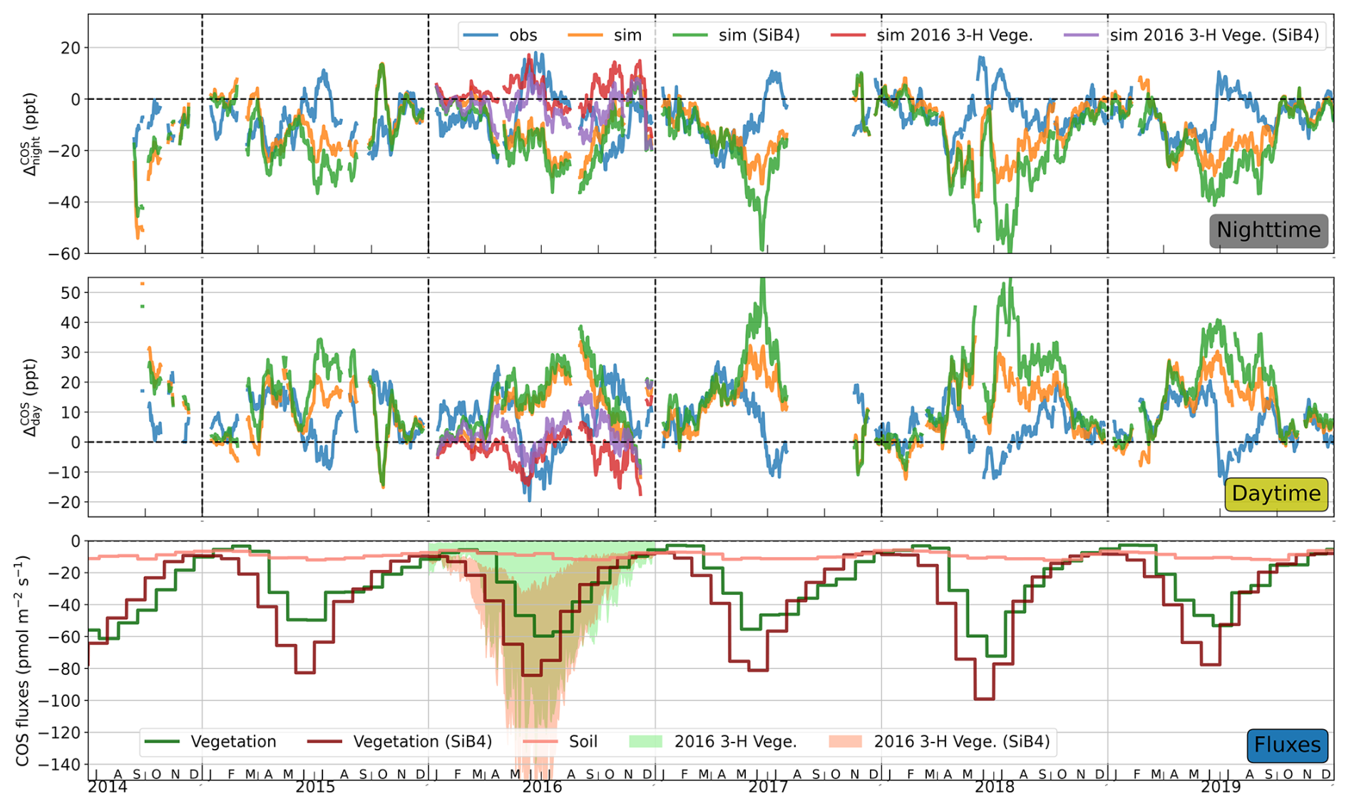
Figure 4 The 15 d rolling mean of the nighttime (${\mathrm{\Delta }}_{\text{night}}^{\text{COS}}$, top) and daytime (${\mathrm{\Delta }}_{\text{day}}^{\text{COS}}$, middle) differences in the observed and simulated COS concentrations at GIF with matching COS total uptake by vegetation and soils in the domain of interest, using the models ORCHIDEE and SiB4 (see Sect. 2.2 for details). Nighttime difference: ${\mathrm{\Delta }}_{\text{night}}^{\text{COS}}$ = [COS]_D@06:00−[COS]_D-1@018:00, daytime difference: ${\mathrm{\Delta }}_{\text{day}}^{\text{COS}}$ = [COS]_D@18:00−[COS]_D@06:00 (see text for more details). Contributions taken into account in the simulations are the background, ocean, our homemade anthropogenic inventory, and either biogenic land with a monthly time resolution (sim) or biogenic land with 2016 3-hourly time resolution for vegetation (sim 2016 3-H Vege.). Fluxes are uptakes by the soil and the vegetation at a monthly (vegetation) or 3-hourly (2016 3-H Vege.) resolution (see Sect. 2.2 for details).

Additional continuous observation sites would be needed in different parts of Europe to clarify the relevancy of our inventory beyond the Paris region and vicinity. In addition, our inventory is based on coarse emission factors, both for the viscose industry and for coal power plants. The facility-level campaign as carried out around a viscose factory near Rouen in Belviso et al. (2023) would significantly improve our understanding of COS anthropogenic fluxes and thus our inventory.

3.3 Biogenic land fluxes

Disentangling the main contribution of mismatches between observations and simulations is very challenging with only one site. Differences at the synoptic scale, as represented in Fig. 1, can originate from an erroneous background, transport discrepancies or incorrect fluxes. Moreover, with only one site, absolute values of the biogenic fluxes cannot be systematically estimated. We therefore focus on the variations through time, particularly between day and night and seasonally. As represented in the time series in Appendix A, fine-scale temporal variability, corresponding to the diurnal cycle, is well reproduced during some periods of the year, especially in spring. The diurnal cycle is dominated by local influences, with remote influence of the background and of distant fluxes transported to GIF filtered out. We therefore focus here on 12 h day or 12 h night differences in measured or simulated COS concentrations, defined as either the “daytime difference”, hereafter ${\mathrm{\Delta }}_{\text{day}}^{\text{COS}}$, between day D at 18:00 and day D at 06:00 or the “nighttime difference”, hereafter ${\mathrm{\Delta }}_{\text{night}}^{\text{COS}}$, between day D+1 at 06:00 and day D at 18:00. Thus, these differences are mostly influenced by a combination of small-scale meteorological conditions (mostly the diurnal cycle of the planetary boundary layer) and of regional fluxes (within the transport footprint around the station). In the present analysis, we assume that all discrepancies are attributable to fluxes, even though the diurnal cycle of transport in FLEXPART is imperfect. Discrepancies in the diurnal cycle of transport patterns would only impact the magnitude of the day–night differences but not the overall patterns discussed below and thus would not impact our qualitative conclusions.

The variations in ${\mathrm{\Delta }}_{\text{day}}^{\text{COS}}$ and ${\mathrm{\Delta }}_{\text{night}}^{\text{COS}}$ over the available 5.5 years of observation are represented in Fig. 4, alongside COS fluxes from regional vegetation and soils, using both the ORCHIDEE and SiB4 models. The observed seasonal cycle of ${\mathrm{\Delta }}_{\text{night}}^{\text{COS}}$ and ${\mathrm{\Delta }}_{\text{day}}^{\text{COS}}$ is similar for all years. The observed ${\mathrm{\Delta }}_{\text{night}}^{\text{COS}}$ is slightly negative in winter (JFM; −7 ppt) and then strongly negative in spring (AMJ; −10 ppt), with yearly peaks of ≈-20 ppt; then, summer positive peaks of 10–15 ppt in July are followed by another negative low in fall (−8 ppt). The positive${\mathrm{\Delta }}_{\text{night}}^{\text{COS}}$ in summer is most probably due to emissions from crops, such as rapeseed (Belviso et al., 2022a). Observed ${\mathrm{\Delta }}_{\text{day}}^{\text{COS}}$ is opposite with slightly different magnitudes.

In winter (JFM), the vegetation is mostly inactive and soils are at their lowest level of sink activity with the net soil uptake becoming larger than the vegetation uptake. Thus the contribution of the uptake by the vegetation and soils in our simulations in both ORCHIDEE and SiB4 for both time resolutions (monthly or 3-hourly) is very small. Both the simulated ${\mathrm{\Delta }}_{\text{night}}^{\text{COS}}$ and ${\mathrm{\Delta }}_{\text{day}}^{\text{COS}}$ are therefore close to zero (on average, −2 ppt for nighttime and +1 ppt for daytime), contrary to observed ${\mathrm{\Delta }}_{\text{night}}^{\text{COS}}$ and ${\mathrm{\Delta }}_{\text{day}}^{\text{COS}}$ (−7 ppt for nighttime and +7 ppt for daytime). This suggests underestimated COS uptakes at night in winter in ORCHIDEE and SiB4 vegetation and/or soil data sets.

During spring (AMJ), vegetation COS uptake is activated in ORCHIDEE and SiB4. When using constant monthly fluxes with no diurnal cycle, their contribution to the simulated nighttime uptake leads to lower concentrations at nighttime compared to daytime, consistent with observations. In contrast, daytime concentrations are the result of compensating vegetation uptake and mixing in the boundary layer. However, the use of 3-hourly vegetation uptake by ORCHIDEE daily cycle results in simulated ${\mathrm{\Delta }}_{\text{night}}^{\text{COS}}$ and ${\mathrm{\Delta }}_{\text{day}}^{\text{COS}}$ close to zero, not consistent with the observations, most likely related to absent uptake at night in ORCHIDEE. On the contrary, in SiB4, persistent uptake occurs at night, leading to more realistic simulation than with ORCHIDEE. This discrepancy suggests a persistent nighttime uptake not adequately represented by ORCHIDEE's diurnal cycle. The ORCHIDEE minimal stomatal conductance at night (see Sect. 2.2.2) has to be revised. Refining the ORCHIDEE model to improve the representation of nighttime processes may enhance its ability to reproduce observed dynamics, compared to SiB4. Summer (JAS) shows opposite behavior compared to spring, with positive nighttime enhancements. These enhancements are not properly reproduced by both ORCHIDEE and SiB4 when using constant monthly fluxes. With 3-hourly fluxes, both models perform well in summer. Using a realistic diurnal cycle is key to reproducing the positive ${\mathrm{\Delta }}_{\text{night}}^{\text{COS}}$ and negative ${\mathrm{\Delta }}_{\text{day}}^{\text{COS}}$. The magnitude of fluxes in ORCHIDEE seems to be in better agreement with observations than with SiB4.

During fall (OND), the performance of our simulations exhibits variability across different years, regardless of the inclusion of a vegetation diurnal cycle. Notably, the simulations for the years 2016 and 2017 show significant discrepancies, whereas the results for the remaining 4 years align well with observational data. This disparity underscores the challenges associated with accurately reproducing the timing of vegetation senescence, particularly given the influence of intricate synoptic meteorological conditions on both vegetation dynamics and the performance of the transport model. The complexity of these interactions poses a significant hurdle in achieving consistent simulation outcomes across all years.

4 Conclusions

The present study analyzes 5.5 years of quasi-continuous COS measurements from the GIF site in the Paris region. At GIF, the seasonal variations in COS mixing ratios are dominated by the contributions of the background and ocean, the weekly to daily variations are driven by the biogenic land contribution, and anthropogenic emissions may dominate for short episodes of high concentrations (Belviso et al., 2023). Through systematic comparison of measurements with simulations using backward trajectories computed with the Lagrangian model FLEXPART, we provide a quantitative assessment of natural and anthropogenic COS fluxes in western Europe.

Regarding industrially emitted COS, we highlight the unrealistic magnitude of anthropogenic fluxes as provided by Zumkehr's inventory (Zumkehr et al., 2018) in Europe. In particular, Zumkehr's inventory suggests very high emissions in the Paris region, inconsistent with the absence of any coal power plants and major viscose industry in the region. We propose another inventory based on reported industrial emissions as well as coal power plants in Europe. The new inventory proves much more consistent with observations and includes only a limited number of emission hot spots in France. Still our inventory comes with several limitations. First, it takes into account the emissions as reported by the “industries”; this category includes only sources above a legally binding threshold. Therefore, we do not account for sources which are under the threshold and we assume them to be small compared to the reported ones; but their overall magnitude actually remains unknown. Second, another limitation arises from the flat temporal variability applied to anthropogenic fluxes in our inventory (similarly to Zumkehr et al., 2018) due to the lack of information on industrial and power-generation activities in viscose factories and coal power plants. This is expected to be a critical limiting factors as coal power plant activity depends on energy demands and viscose industrial activity is often organized by batches with days of intense emissions followed by periods with limited emissions. Third, we apply a single emission factor between CO₂ and COS emissions from coal power plants, whereas this factor depends on the coal used in the combustion, as well as the overall properties and technologies used in the power plant. Last, limitations are also due to the model-based approach of our study. The sources of COS or its precursors are stacks of factories or coal power plants, i.e., hot spots: high-emission sources localized in a very small area compared to the resolution of the chemistry-transport model used to simulate the concentrations. Therefore, the plumes emitted from these hot spots are not always well represented by the model, depending on the meteorological situation. For hot spots close to the measurement site (e.g., from the Beauvais region 50 km north of GIF, where viscose factories are active), the numerical diffusion of the plumes of COS represented in the model leads most of the time to underestimating simulated concentrations; in particular events, if the error in the wind direction is large enough, the plume may be unduly directed to the site in the model, which leads to overestimating the simulated concentrations. Overcoming the above-mentioned limitations in assessing anthropogenic emissions would mostly need additional observation sites in the region (e.g., Zanchetta et al., 2023, in the Netherlands) to cross-validate our results.

For anthropogenic and oceanic CS₂ emissions, the kinetics of the conversion of CS₂ into COS through its oxidation by OH is not well known. Moreover, through OH availability and temperature, the lifetime of CS₂ depends on the season and has a diurnal cycle. The impacts of these variations on the chemical source of COS must be assessed, when more relevant information, e.g., varying diurnal emissions, is available.

Regarding soil and vegetation fluxes, we are able to suggest that the net ecosystem COS uptake simulated by both ORCHIDEE and SiB4 is underestimated in winter at night, requiring improvements in the nighttime processes in land process models. The uncertainties in the modeling of transport at night in winter prevent us from quantifying the underestimation of the nighttime COS uptake. However, the discrepancies between simulations and observations shown by the nighttime and daytime differences suggest the existence of such an underestimation. Even when using ORCHIDEE's vegetation and soil uptakes with a diurnal cycle at a 3-hourly resolution, the analysis of the simulated diurnal cycle of COS concentrations confirms that a nighttime uptake is not adequately represented by ORCHIDEE, maybe due to the parameterization of the nighttime uptake by plants for COS. Opposite to that, SiB4 has a more realistic representation of spring diurnal cycles of fluxes, leading to better agreement between simulations and observations of concentrations. In summer, the magnitude of fluxes by ORCHIDEE is more consistent than SiB4 fluxes when comparing to observations. Further work is needed to properly compare ORCHIDEE and SiB4 using day–night differences as the FLEXPART model is imperfect regarding the representation of the diurnal cycle of transport and dispersion. An analysis discriminating between the impacts of (i) the fluxes, (ii) the chemical source, (iii) the vertical transport and (iv) the advection on COS mixing ratios could be performed from a set of simulations, with a careful design, computer resources and up-to-date hourly varying fluxes. Replicating our study with another transport model and other meteorological constraints would allow for assessing the uncertainty in diurnal simulations; even these uncertainties would only impact the magnitudes of the simulations and not their patterns, hence leading to unchanged conclusions.

Although it is based on only one site, the present study provides sufficient elements to identify discrepancies in COS emission databases and land process models in western Europe, due to incorrect parameterizations of fluxes or missing processes. Still, our single-site study is not sufficient to overcome those discrepancies to reach the level of precision needed to use COS observations as a proxy for plant uptake. A full network of observation sites, analog to the Integrated Carbon Observatory System (ICOS; Ramonet et al., 2011), would be a requirement to better quantify anthropogenic fluxes and thus to fully use COS for assessing CO₂ uptake by photosynthesis.

Appendix A: Time series of observations and simulations

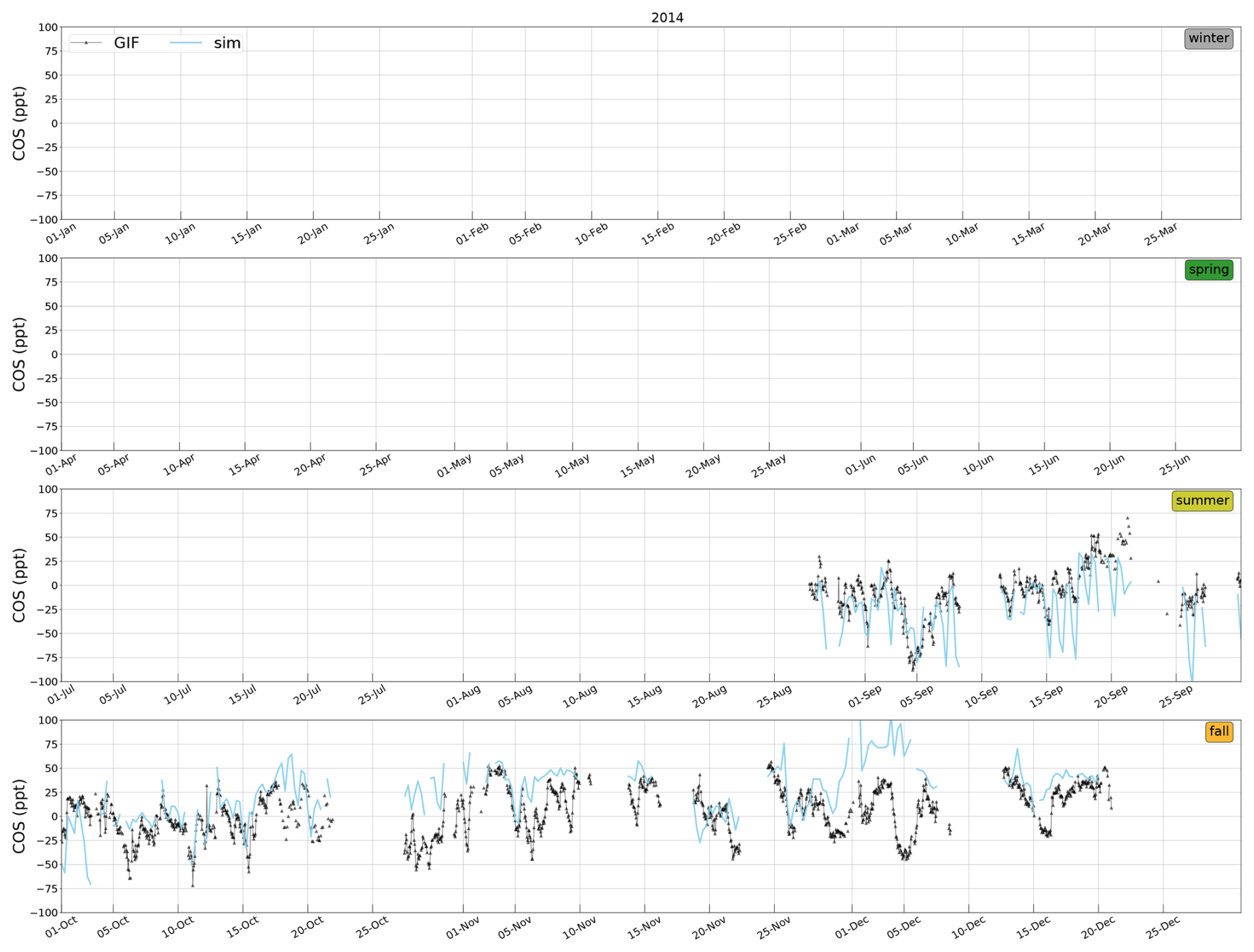
Figure A1 Smoothed time series of observed and simulated atmospheric mixing ratios of COS at GIF in 2014. Observations are hourly averages. Contributions taken into account in the simulations are the background, ocean, our homemade anthropogenic inventory, and biogenic land with a monthly time resolution for vegetation and soils (see Sect. 2.2 for details). Smoothed by subtracting the rolling 20 d mean of the observations to the observed and simulated time series. Note that the time series begins at the end of August 2014.

Figure A2 Same as Fig. A1 for the year 2015.

Figure A3 Same as Fig. A1 for the year 2016, with simulated contribution from the vegetation uptake with 3-hourly time resolution (see Sect. 2.2 for details).

Figure A4 Same as Fig. A1 for the year 2017.

Figure A5 Same as Fig. A1 for the year 2018.

Figure A6 Same as Fig. A1 for the year 2019.

Appendix B: Contributions to COS mixing ratios at GIF

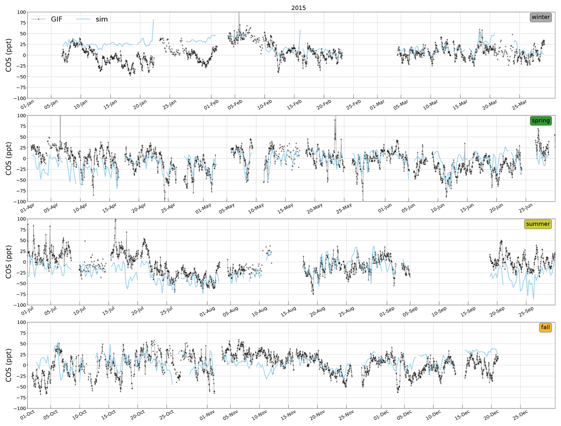
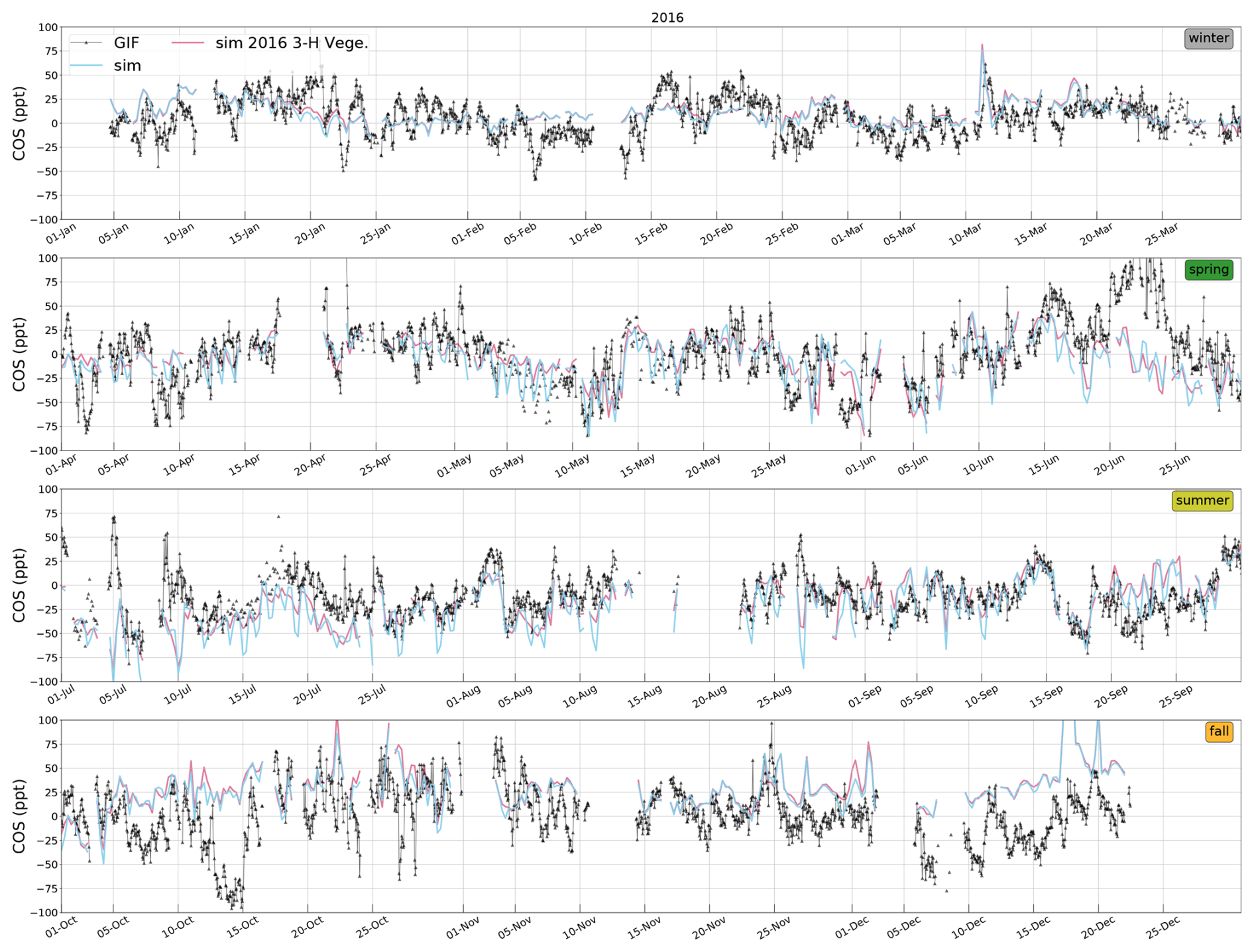
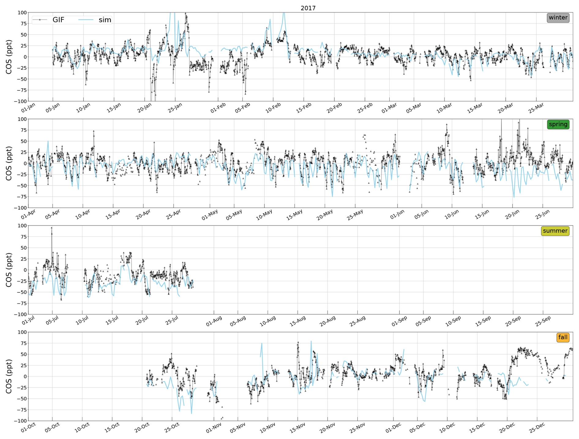
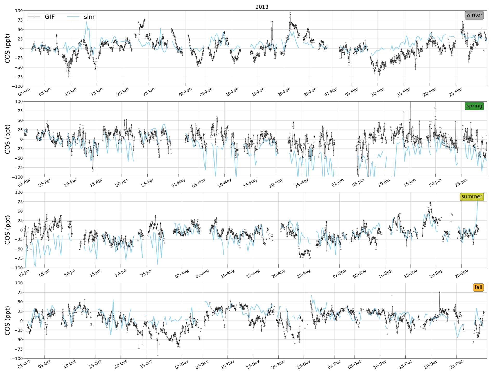
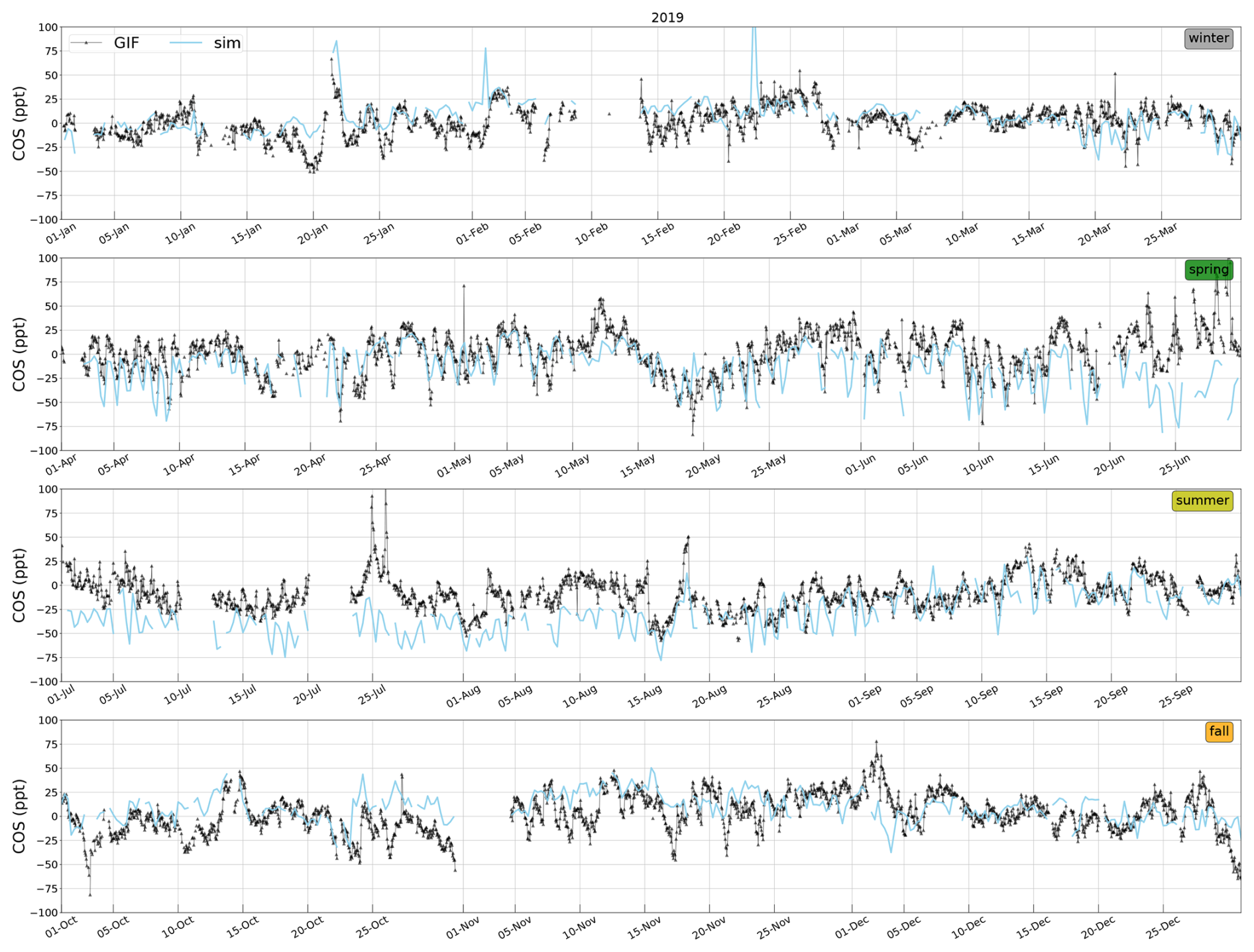
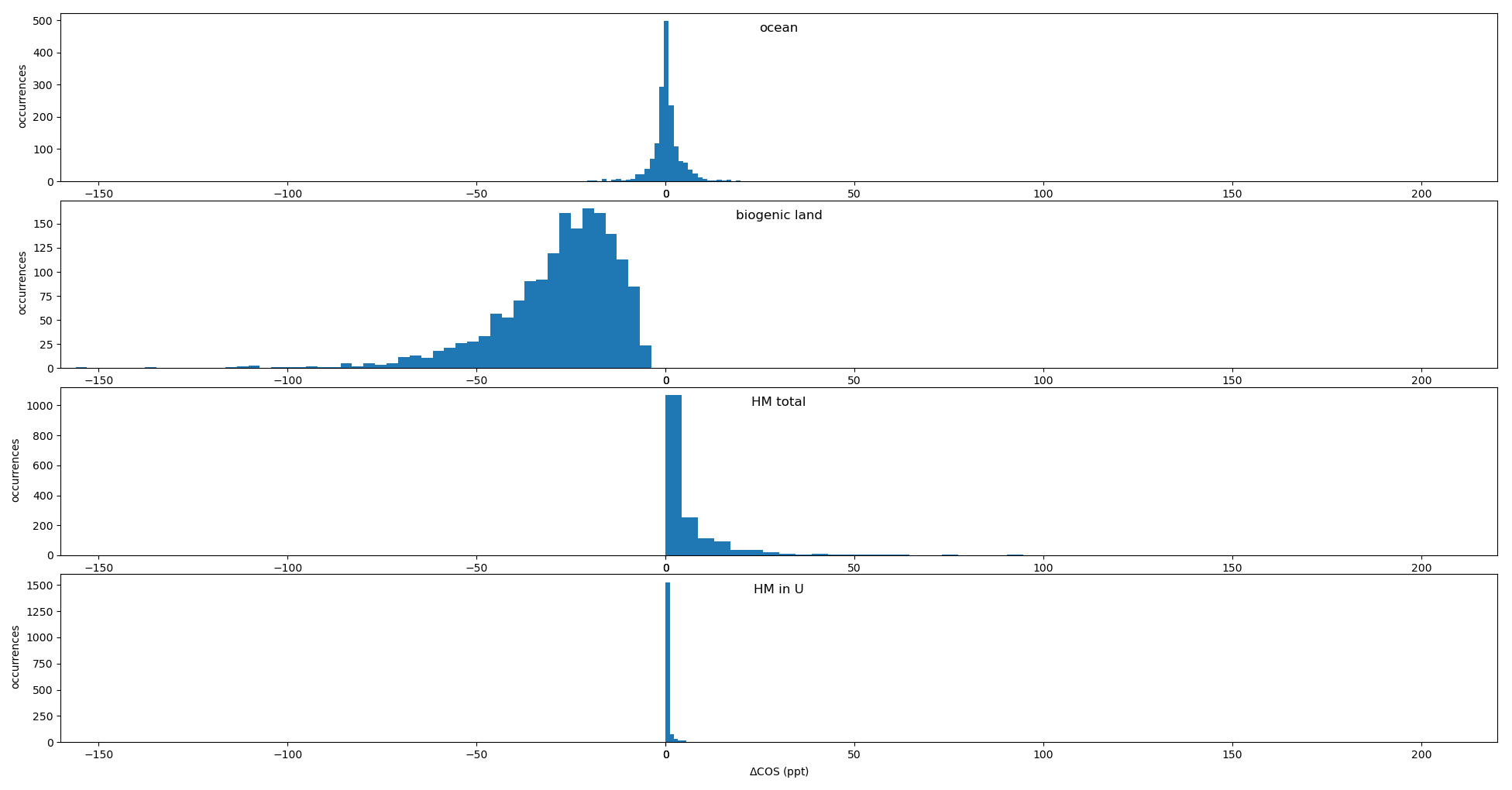
Figure B1 Occurrences of contributions (ΔCOS, in ppt) to COS mixing ratios at GIF due to the background, the ocean, the vegetation and soil (biogenic land), and our homemade anthropogenic emissions (total and only the Paris and Rouen area). Total number of occurrences: 1673 simulated values matching afternoon (12:00–18:00 UTC) valid mean observations between 2014 and 2019.

Appendix C: Statistical indicators of the performance of the model compared to the measurements at GIF for each contribution

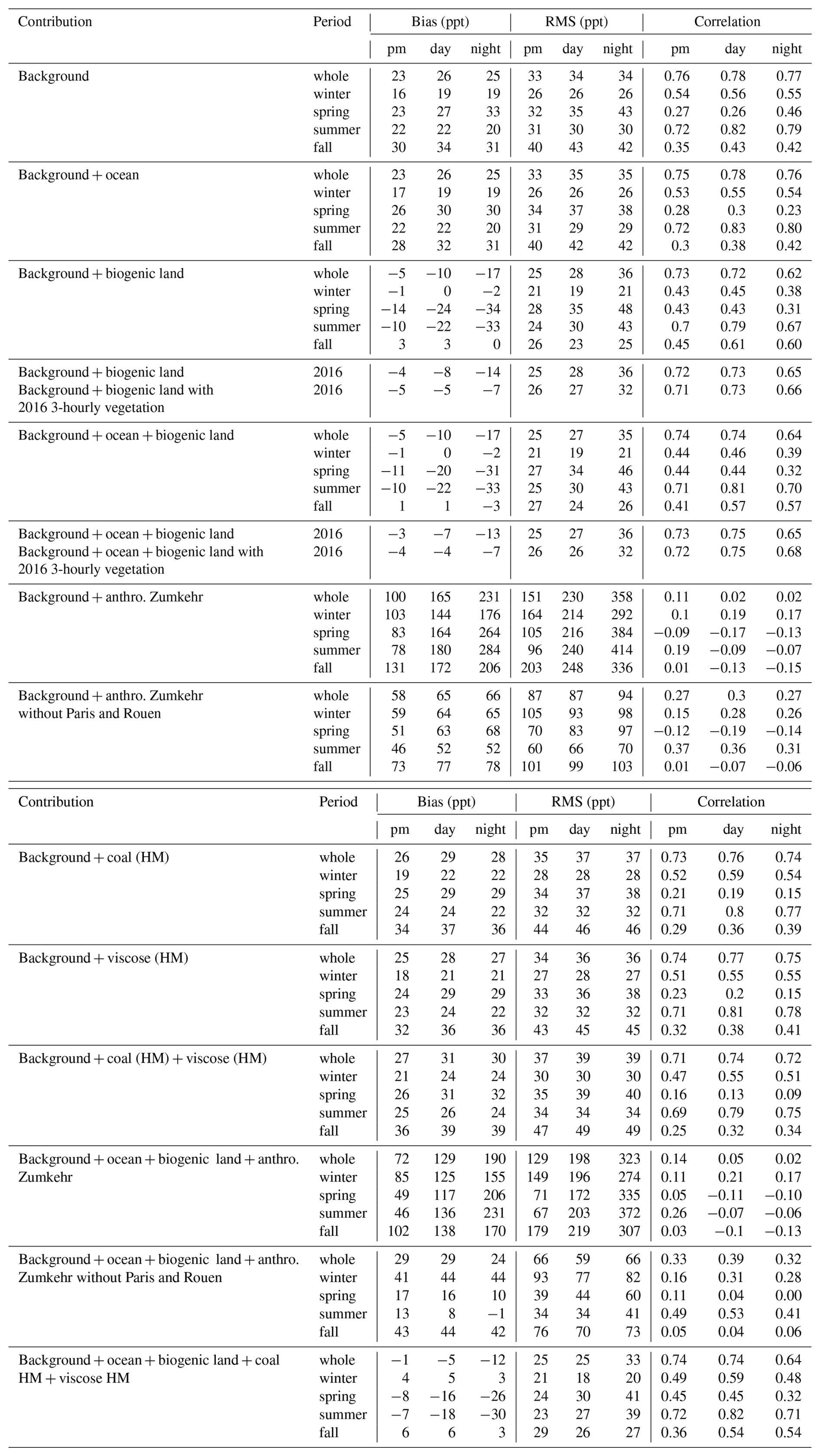
Table C1 Statistical indicators of the performance of the model compared to the measurements at GIF for each contribution. Indicators are either computed over the whole period, i.e., August 2014–December 2019 (see Sect. 2.1, whole); separated into four seasons (winter: January, February, March; spring: April, May, June; summer: July, August, September; fall: October, November, December); or computed only over the year 2016 for comparison with the available contribution by the 3-hourly varying vegetation. For each period, the means are during the afternoon (12:00–18:00 UTC, pm), the whole day (day) or nighttime (21:00–02:00 UTC, night). Bias: mean difference model minus measurement, RMS: root mean square model minus measurements, correlation: Pearson's correlation coefficient between model and measurement time series. HM indicates emissions from our homemade inventory (see Sect. 2.2.3).