Australian bushfire emissions result in enhanced polar stratospheric clouds

Extreme bushfire events amplify climate change by emitting greenhouse gases and destroying carbon sinks. They also cause economic damage, through property destruction, and even fatalities. One such bushfire occurred in Australia in 2019–2020, and this event injected large amounts of aerosols and gases into the stratosphere and depleted the ozone layer. While previous studies have focused on the drivers behind ozone depletion, the bushfire impact on polar stratospheric clouds (PSCs), a paramount factor in ozone depletion, has not been extensively investigated so far. Therefore, this study focuses on the effects of bushfire aerosols on the dynamics and stratospheric chemistry related to PSC formation and its pathways. An analysis from Aura's Microwave Limb Sounder revealed that the enhanced hydrolysis of dinitrogen pentoxide significantly increased nitric acid (HNO₃) in the high-latitude lower stratosphere in early 2020. This resulted in an anomalously high areal coverage of PSCs with ice, exceeding 3 standard deviations with respect to background period. Based on Lagrangian backward-trajectory analysis, we find that a predominant fraction (79 %) of the liquid–nitric acid trihydrate (NAT) mixture formed via the ice-free nucleation pathway. These NAT particles subsequently acted as nuclei for ice formation, accounting for 95 % of the observed ice PSCs. This rapid conversion from NAT to ice likely contributed to the strong positive anomaly in ice PSC. This highlights the primary formation pathways of ice and liquid–NAT mixtures and possibly helps us to simulate PSC formation and denitrification process better in climate models. These findings will contribute significantly to a deeper understanding of the impacts of extreme wildfire events on stratospheric chemistry and PSC dynamics.

1 Introduction

Southeast Australia, comprising the states of New South Wales and Victoria, faced an extreme bushfire event from September 2019 to February 2020. This bushfire occurrence has been widely recognized as the “Black Summer” or “Australian New Year” (ANY) event and has been extensively studied (Allen et al., 2020; Deb et al., 2020; Schwartz et al., 2020; Chang et al., 2021; Rieger et al., 2021; Tencé et al., 2021, 2022; Heinold et al., 2022; Sellitto et al., 2022). This catastrophic event injected substantial amounts of aerosols, between 0.4 and 2 Tg, into the lower stratosphere of the Southern Hemisphere (Khaykin et al., 2020; Hirsch and Koren, 2021; Heinold et al., 2022; Tencé et al., 2022); these emissions were composed of 2.5 % black carbon and 97.5 % organic carbon (Yu et al., 2021). Significant warming of the midlatitude stratosphere by up to 3.5 K was reported; prior to this event, a midlatitude stratospheric warming of this magnitude had not been observed since the 1991 eruption of Mount Pinatubo (Stocker et al., 2021). Additionally, this event led to significant changes in the abundance of various trace gas species, such as CH₄, CO, CH₃CN, CH₃Cl, HCN, CH₃OH, HCl, HNO₃, H₂O, and ClONO₂, particularly in the midlatitude lower stratosphere (Schwartz et al., 2020; Santee et al., 2022; Wang et al., 2023).

Furthermore, these aerosols provided a surface area for heterogeneous chlorine activation reactions to occur, resulting in the early depletion of HCl and an enhancement of ClO (Santee et al., 2022), and led to additional stratospheric ozone loss (Solomon et al., 2022). Along with these aerosols, liquid polar stratospheric clouds (PSCs) are also known to promote such ozone-depleting heterogeneous reactions (Molina et al., 1993; Carslaw et al., 1994; Ravishankara and Hanson, 1996). Solid PSCs, such as nitric acid trihydrate (NAT), are known to retard the deactivation process of active halogens like chlorine, bromine, and fluorine through denitrification and, thereby, contribute to prolonged ozone depletion (Hoyle et al., 2013). Ansmann et al. (2022) reported that the bushfire aerosols from the Black Summer event influenced PSCs by increasing their surface area and particle number concentration. Wang et al. (2023) reported an increased stratospheric chlorine activation on the bushfire aerosols and PSCs. However, previous studies have not extensively investigated the influence of the Black Summer event on PSC dynamics. It is crucial to understand the influence of extreme events like the Black Summer on PSC dynamics for two main reasons:

• (i)

  The frequency of extreme wildfire events is projected to increase due to global warming (Mansoor et al., 2022), resulting in the increased injection of aerosols into the stratosphere, which could enhance the PSC areal coverage.

• (ii)

  Stratospheric cooling is anticipated to further expand PSC coverage, resulting in more surface area density for chlorine activation reactions and, thus, more ozone depletion (e.g., Khosrawi et al., 2016; Thölix et al., 2016; Robrecht et al., 2019).

On the above backdrop, using multi-satellite measurements and reanalysis data, this study aims to investigate the anomalies in stratospheric chemistry and PSC dynamics caused by the Black Summer event. This remainder of this paper is structured as follows: we review PSCs and their formation pathways relevant to the current study (Sect. 2), detail the data and methodology used (Sect. 3), provide the results and a discussion (Sect. 4), and conclude the study (Sect. 5).

2 Brief literature review of PSCs

The stratosphere contains a widespread presence of sulfate aerosols composed of sulfuric acid and water (Junge et al., 1961). It receives an influx of 160 t d⁻¹ of sulfur from the troposphere, which corresponds to the production of 650 t d⁻¹ of aqueous sulfuric acid (Thomason and Peter, 2006). In addition to the sulfate aerosols, meteoritic dust particles of extraterrestrial origin contribute 20–100 t d⁻¹ (Cziczo et al., 2001), making up 3 %–15 % of the total mass of stratospheric aerosols. These dust particles are carried by the Brewer–Dobson circulation and funneled from the mesosphere into the stratospheric polar regions of both hemispheres during the formation of the polar vortex (Engel et al., 2013). As winter approaches, the absence of solar radiation in the polar regions leads to a significant decrease in temperature, creating conditions conducive to trace gases such as HNO₃ and H₂O to condense onto stratospheric aerosols, forming PSCs (Carslaw et al., 1994; Voigt et al., 2000). Hence, these PSC particles predominantly consist of HNO₃, H₂SO₄, and H₂O (Lowe and MacKenzie, 2008; Peter, 1997). It is hypothesized that stratospheric sulfuric acid aerosols containing meteoritic dust could also serve as nuclei for PSC formation (Bogdan et al., 2003; Bogdan and Kulmala, 1999; Murphy et al., 2014; Schneider et al., 2021).

2.1 Types of PSCs

PSCs exist in both liquid and solid form in the lower stratosphere. Supercooled ternary solution (STS) PSCs comprise a liquid PSC type with an equal proportion of H₂SO₄, HNO₃, and H₂O, and they form at T_ice+3 K (Carslaw et al., 1994). Nitric acid trihydrate (NAT) PSCs are comprised of solid particles with a proportion of 1 HNO₃ and 3 H₂O, and they form at T_ice+4 K (Hanson and Mauersberger, 1988). Finally, ice PSCs form through homogeneous nucleation at T_ice−3 K (Carslaw et al., 1998; Koop et al., 1998) and via the heterogeneous nucleation of ice at T_ice−0.1 to 1.5 K (Koop et al., 1998, 2000; Fortin et al., 2003; Engel et al., 2013). STS assists in chlorine activation by providing surface area, resulting in pronounced ozone depletion, and NAT is involved in denitrification, leading to prolonged ozone depletion (Molina and Rowland, 1974; Molina et al., 1993; Ravishankara and Hanson, 1996; Waibel et al., 1999; Hoyle et al., 2013).

2.2 PSC formation pathways

2.2.1 NAT formation pathways

The homogeneous nucleation of NAT is kinetically suppressed (Koop et al., 1995). Laboratory experiments have revealed that the homogeneous nucleation rate of NAT on liquid STS is extremely low under stratospheric conditions (Hanson and Ravishankara, 1991, 1992). Thus, NAT forms through heterogeneous nucleation processes such as (i) ice-assisted NAT nucleation and (ii) ice-free NAT nucleation. During the ice-assisted NAT nucleation process, the ice particles serve as nuclei for NAT formation upon warming of the air parcels, and this occurs at a high saturation ratio over NAT of > 500 (Luo et al., 2003). This mechanism has been supported by several field observations (Carslaw et al., 1999) and by bulk-phase lab experiments (Koop et al., 1995, 1997), which indicated that the deposition nucleation of NAT on exposed ice surfaces is also a possible pathway for NAT formation. During the ice-free NAT nucleation, instead of ice, STS with solid foreign nuclei inclusion, such as meteoritic dust, volcanic ash, soot, or H₂SO₄ hydrates, serves as a NAT nucleus (Iraci et al., 1995; Koop et al., 1997; Peter and Grooß, 2012), and this even occurs at a low saturation ratio over NAT (S_NAT) of <10 (Voigt et al., 2005). Hoyle et al. (2013) made a new parameterization scheme for NAT nucleation on foreign nuclei in the immersion mode and reproduced the CALIPSO PSC observations for the entire Arctic winter of 2009–2010.

2.2.2 Ice formation pathways

Ice PSCs can form either homogeneously under high-supersaturation conditions, with a saturation ratio over ice (S_ice) > 1.5, at a temperature of 3 K less than the frost point (T_ice) (Koop et al., 1998) or heterogeneously on STS with foreign nuclei inclusion at a temperature of 1.5 K less than T_ice (Koop et al., 1998, 2000; Engel et al., 2013). Apart from these foreign nuclei, NAT is also known to act as potential nucleus for ice formation (Gao et al., 2016; Hanson and Mauersberger, 1988; Iannarelli and Rossi, 2015; Khosrawi et al., 2011; Weiss et al., 2016). Based on the WALES (Water Vapor Lidar Experiment in Space – airborne demonstrator) lidar aboard HALO (High Altitude and Long Range Research Aircraft), Voigt et al. (2018) showed that the depolarization ratio of ice PSCs exhibited a bimodal distribution: the low depolarization mode corresponds to the ice nucleated on STS with foreign nuclei inclusion, whereas the high depolarization mode corresponds to the ice nucleated on NAT particle. Engel et al. (2013) made a new parameterization scheme for ice nucleation on foreign nuclei in immersion mode and reproduced the CALIPSO PSC observations for the entire Arctic winter of 2009–2010.

In the present study, along with investigating the impact of the Black Summer event on lower-stratospheric chemistry, in order to explain the observed PSC anomalies, we also aim to quantify the percentage of the liquid–NAT mixture formed via the ice-assisted and ice-free nucleation processes. Furthermore, we quantify the percentage of ice PSC that nucleates on NAT (NAT-assisted nucleation pathway) and STS (NAT-free nucleation pathway).

3 Data and methodology

3.1 Satellite and reanalysis data

The Ozone Monitoring Profiler Suite (OMPS) aboard the Suomi NPP and NOAA-20 satellites measures atmospheric O₃ and aerosols using limb-viewing techniques. We have used the OMPS level 2, version 2.0 product; this product provides the aerosol extinction coefficient at 745 nm wavelength, with a horizontal resolution of 125 km × 2 km and a vertical resolution of 1.8 km (https://disc.gsfc.nasa.gov/datasets/OMPS_NPP_ LP_ L2_ AER_DAILY_2/summary, last access: 6 July 2025; Taha et al., 2021).

The Microwave Limb Sounder (MLS) aboard the Aura satellite provides trace gas mixing ratios by measuring limb emission spectra through a five-band microwave radiometer. We have used the MLS Level 2, version 5.0 daily HNO₃ and H₂O mixing ratios (https://mls.jpl.nasa.gov/eos-aura-mls/data.php, last access: 6 July 2025; Waters et al., 2006) for the present study.

The Atmospheric Chemistry Experiment Fourier transform spectrometer (ACE-FTS) aboard the SciSat satellite provides trace gas mixing ratios by measuring limb absorption spectra and level 2, version 4.0 daily HF, H₂O, HNO₃, and N₂O₅ mixing ratios (https://www.frdr-dfdr.ca/repo/dataset/a1deafb8-0888-82e8-7dd5-b46c58092683, last access: 6 July 2025; Bernath et al., 2020).

The Cloud–Aerosol Lidar with Orthogonal Polarization (CALIOP) instrument aboard the Cloud–Aerosol Lidar and Infrared Pathfinder Satellite Observations (CALIPSO) satellite probes the vertical distribution of aerosols and clouds (Pitts et al., 2007). It classifies PSCs, using the perpendicular attenuated backscatter and total scattering ratio (ratio between the total attenuated backscatter to the molecular backscatter), into five categories: supercooled ternary solution (STS ≡ H₂SO₄ ⋅ HNO₃ ⋅ H₂O), liquid–nitric acid trihydrate mixtures (liquid–NAT mixtures ≡ HNO₃.3H₂O, a mixture of liquid STS and solid NAT with a low number density of 10⁻² cm⁻³), enh. NAT (enhanced NAT with a high number density of 10⁻¹ cm⁻³), ice (water ice ≡ H₂O), and mountain wave ice (MWI ≡ H₂O, caused by gravity waves). The total areal coverage values of PSCs such as liquid–NAT mixtures, STS, ice, enh. NAT, and MWI are 48 %, 24.7 %, 21.4 %, 5.8 %, and 0.1 %, respectively (Pitts et al., 2018). However, these values are subject to interannual variation, modulated by the polar vortex dynamics. In addition, gas-phase HNO₃ is observed from the Microwave Limb Sounder (MLS) from March to April every year. The backscattered signals from the sub-visible PSCs which are NAT particles with an extremely low number density, are well below the detection threshold of the CALIPSO receiver. Hence, CALIPSO classifies these grids as “No Cloud (NC)” (Lambert et al., 2012) during this period. Thus, the CALIPSO NC grid indicates either no presence of PSCs or the presence of sub-visible PSCs. In this study, CALIPSO PSC Level 2, version 2.0 is used (https://asdc.larc.nasa.gov/project/CALIPSO/CAL_LID_L2_PSCMask-Standard-V2-00_V2-00, last access: 6 July 2025; Pitts et al., 2007, 2009, 2013); this product provides PSC information at a spatial resolution of 180 m along the flight track and 500 m perpendicular to the track. The PSC areal coverage is estimated as described in Pitts et al. (2009).

The European Centre for Medium-Range Weather Forecasts fifth-generation (ERA5) reanalysis provides meteorological data with a spatial resolution of 0.25° × 0.25° and a temporal resolution of 1 h at 37 pressure levels (1000 to 1 hPa). We have used the hourly meridional and zonal velocity from June to July 2020 (https://cds.climate.copernicus.eu/datasets/reanalysis-era5-pressure-levels?tab=overview; last access: 6 July 2025; Hersbach et al., 2020).

3.2 Anomaly estimation

Anomalies (Δ) in the aerosol extinction coefficient (k_ext at 745 nm), mixing ratios of H₂O and HNO₃, and PSC properties (such as areal coverage and volume) are estimated following Eq. (1):

$$\begin{array}{}\text{(1)}& \mathrm{\Delta }X=X_{\mathrm{2020}}-\stackrel{\mathrm{‾}}{X},\end{array}$$

where ΔX is a daily anomaly in quantity X, X₂₀₂₀ is the daily mean in 2020, and $\stackrel{\mathrm{‾}}{X}$ is the daily background mean. The background mean values of the H₂O and HNO₃ mixing ratios and PSC properties are constructed by averaging the daily values during the period from 2009 to 2019, whereas for k_ext, the period is from 2012 to 2019 (excluding the year 2015 in order to avoid the effects of the Calbuco volcanic eruption; Zhu et al., 2018). The standardized anomaly (Z) is estimated following Eq. (2):

$$\begin{array}{}\text{(2)}& Z{}_X={\displaystyle \frac{\mathrm{\Delta }X}{{\mathit{\sigma }}_X}},\end{array}$$

where σ_X is the standard deviation of the parameter X.

3.3 Methodology for retrieval of formation pathways

To retrieve the formation pathways of the PSCs, knowledge of the temperature history of the corresponding air parcel is crucial (Larsen et al., 1997). Hence, using the Chemical Lagrangian Model of the Stratosphere (CLaMS) trajectory module, the backward trajectories of the air parcels containing ice and liquid–NAT mixture PSCs are calculated. The methodology is similar to that of previous studies that retrieved PSC formation pathways from CALIPSO (Nakajima et al., 2016) and from aircraft campaigns (Voigt et al., 2018) using Lagrangian trajectory analysis. The current methodology employed in this paper has three steps: (i) selection of ice and liquid–NAT mixture PSCs, (ii) Lagrangian backward-trajectory analysis, and (iii) determination of the change in PSC composition. These three steps are described below (Sect. 3.3.1–3.3.3).

3.3.1 Selection of ice and liquid–NAT mixture PSCs

As liquid–NAT mixture and ice are the first (with 48 %) and third (with 21.4 %) most abundant types of PSCs in terms of areal coverage (Pitts et al., 2018), performing backward trajectories for all of these detected PSC types is computationally expensive. Furthermore, the ERA5 operational analysis data are available at a temporal resolution of 1 h, whereas CALIPSO's temporal resolution is one profile per second. The accuracy of the trajectory relies on the accuracy of the wind field and diabatic heating rate. Hence, assigning an hourly wind field and diabatic heating rate to all CALIPSO profiles measured during the specific hour may contribute to uncertainty in the calculated trajectory. Although the degree of uncertainty is unclear, as a conservative measure, we impose another criterion to minimize any uncertainty that may contribute. Thus, the two criteria utilized are as follows:

• Criteria 1. Firstly, CALIPSO profiles that are measured within 5 min of (before and after, i.e., 10 min time windows) any hour of the ERA5 operational analysis data are chosen. For instance, if ERA5 operational analysis data are available for the time 01:00 UTC for a specific day, CALIPSO profiles measured between 12:55 and 01:05 UTC on the same day are considered.

• Criteria 2. Secondly, from these chosen profiles, an ice PSC grid (liquid–NAT mixture PSCs) is chosen only if all of its surrounding grids are classified as ice PSCs (liquid–NAT mixture PSCs) i.e., the 3×3 CALIPSO grids should be homogeneously populated by either ice or a liquid–NAT mixture.

3.3.2 Lagrangian backward-trajectory analysis

The backward trajectories for these selected grid points are calculated for a 48 h period using the CLaMS trajectory module. The rationale behind choosing 48 h is that, once the air parcel's temperature drops below T_NAT and following the nucleation of NAT particles with a number density of $\mathrm{5}\times {\mathrm{10}}^{-\mathrm{4}}$ to $\mathrm{5}\times {\mathrm{10}}^{-\mathrm{5}}$ cm⁻³, the NAT particles exceed the CALIPSO perpendicular backscatter threshold and become detectable within ∼ 19 h (0.8 d) (Lambert et al., 2016). Similarly, Voigt et al. (2005) provided observational evidence from aircraft campaigns showing NAT formation within approximately 20 h after the temperature drops below T_NAT. In the case of ice formation, a 48 h period should be sufficient, considering the average cooling rate in the stratosphere. The model runs are driven by meteorological data from the ERA5 operational analysis, with a temporal resolution of 1 h and a spatial resolution of 1° × 1°. The time step is set to 60 s in the CLaMS trajectory module. The vertical coordinate is potential temperature. The vertical motion of the air parcels is modulated by total diabatic heating rates derived from ERA5, following Ploeger et al. (2021).

3.3.3 Determination of the change in PSC composition

To determine the PSC composition along each trajectory, we first identify the intersection points where the trajectory intersects with the CALIPSO scan track, with a temporal coincidence of ±30 min. Intersections with time differences exceeding this threshold are disregarded, thereby ensuring that the trajectory and CALIPSO scan track are both spatially and temporally co-located within a 30 min time window. The PSC composition at each trajectory intersection point is then determined from the CALIPSO measurement profile with a potential temperature closest to that of the trajectory's intersecting point. If the PSC composition determined in this manner differs from the initial composition observed at the start of the trajectory (i.e., at time t=0 h), we assign this PSC composition to the intersection point of the trajectory. Conversely, trajectories with no change in PSC composition are excluded from further consideration. Moreover, we fill the MLS-observed HNO₃ and H₂O mixing ratios along the selected trajectories to study the uptake of these gases during PSC formation.

Following the above three steps, we chose a total of 8841 backward trajectories. Of these, 3792 trajectories correspond to a liquid–NAT mixture, whereas the remaining 5049 trajectories correspond to ice PSCs. Each trajectory contains the temperature from the ERA5 operational analysis, HNO₃ and H₂O mixing ratios from MLS at the points where the trajectories intersect with the CALIPSO scan track, and the PSC composition from CALIPSO. In addition, derived quantities such as T_ice, T_NAT, ice and NAT surface area density from the CLaMS box model run, S_NAT (for the case of backward trajectories of liquid–NAT mixture), and S_ice (for the case of backward trajectories of ice) are added to the trajectories. Hence, this provides a comprehensive picture of the air parcels' temporal evolution leading to the formation of liquid–NAT mixture and ice PSCs.

3.4 CLaMS microphysical modeling of the observed uptake of HNO₃ and H₂O

The ice and liquid–NAT mixture PSCs form through the condensation/deposition of gas-phase HNO₃ and H₂O under cold stratospheric conditions, leading to their depletion. To check the reliability of the retrieved PSC formation pathways (as discussed in Sect. 3.3), we used the CLaMS microphysical box model to validate the MLS-observed uptake of these gases with the CLaMS-modeled uptake during the formation of the PSCs. CLaMS is a chemical transport model developed by the Forschungszentrum Jülich in Germany (McKenna et al., 2002a, b). It has several modules, such as chemistry (McKenna et al., 2002b), mixing (McKenna et al., 2002a), trajectory (Konopka et al., 2004), and sedimentation (Grooß et al., 2005, 2014; Tritscher et al., 2019), which collectively help simulate stratospheric chemistry, PSC formation, and ozone depletion.

In the present study, we utilized the trajectory module and microphysical box model from the chemistry module. First, the liquid–NAT mixture/ice PSC is selected (as discussed in Sect. 3.3.1) and its backward trajectory is estimated (as discussed in Sect. 3.3.2). Following this, the intersection of the trajectory with the CALIPSO scan track is identified (as discussed in Sect. 3.3.3). As the CALIPSO PSC product comes with MLS observations interpolated to the CALIPSO grids, the beginning and end of the trajectory have MLS HNO₃ and H₂O. The intersection of the backward trajectory with the CALIPSO scan track is considered to be a beginning point and is fed into the CLaMS microphysical box, i.e., the trajectory starts at time t<0 h and ends at time t=0 h. The inputs for the box model run are trajectory coordinates (time, latitude, longitude, and potential temperature), temperature and pressure along the trajectories, and MLS-observed HNO₃ and H₂O mixing ratios at the beginning of the trajectory. The mixing ratios of the rest of the gases are set to 0; hence, other chemical reactions, such as chlorine activation, HCl null cycles, and N₂O₅ hydrolysis, are not considered. In the box model run, T_ice is estimated following the equations provided by Marti and Mauersberger (1993), while T_NAT is estimated following Hanson and Mauersberger (1988).

4 Results and discussion

4.1 Increased aerosol loading in the lower stratosphere

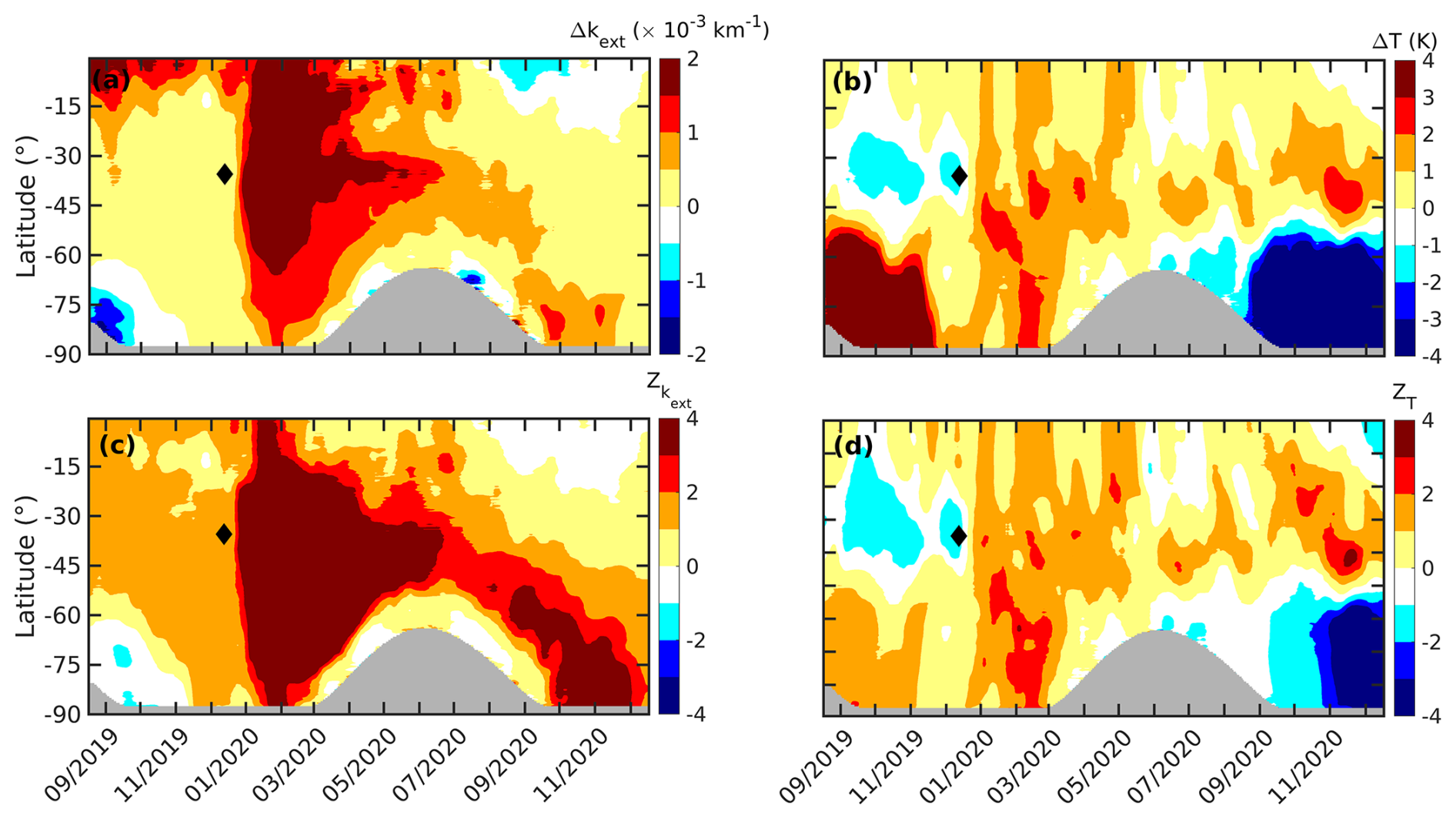
Figure 1 The daily zonal mean anomaly (Δ) in OMPS (a) k_ext at 745 nm and (b) temperature and the standardized anomaly (Z) in (c) k_ext at 745 nm and (d) temperature at an altitude of 15 km between September 2019 and December 2020 are shown. The gray-shaded region corresponds to no data. The ticks on the x axis mark the middle of each month. The black diamond in each plot marks the Black Summer event.

An anomaly in the aerosol extinction coefficient (k_ext) at 745 nm derived from cloud-filtered OMPS observations and an anomaly in temperature, along with their corresponding standardized anomalies, at an altitude of 15 km are shown in Fig. 1. A notable positive anomaly in k_ext in the midlatitude from early January in 2020 is attributable to the increased aerosol loading caused by the Black Summer event (Fig. 1a). The anomaly in k_ext exceeded 3 standard deviations (Fig. 1c) and warmed the lower stratosphere by 2 K due to radiative heating (Rieger et al., 2021), which is readily seen in Fig. 1b. By February 2020, these aerosols had been transported to high latitudes where PSCs usually form in the subsequent Austral winter. As stratospheric aerosols act as nuclei for PSCs, it is likely that these aerosols also influenced the PSC dynamics during this period. A negative anomaly in k_ext is observed at a latitude of $\sim -\mathrm{80}$° from April 2020, and this is attributed to the nucleation of PSC on these aerosols (Zhu et al., 2018). The k_ext increased again at high latitudes in October and November 2020 due to the rerelease of the captured aerosols by the PSC, upon evaporation of the corresponding gas species (Toon et al., 1989; Schwarzenböck et al., 2001; Rex et al., 2004; Hoyle et al., 2013). Previous studies have reported additional ozone loss during the same period (Ansmann et al., 2022; Ohneiser et al., 2022). Despite the abundant aerosol loading, strong cooling of more than 3 K was observed in high-latitude regions from September to December 2020 (Fig. 1b). This suggests that the radiative cooling caused by the additional ozone loss (Fig. S1 in the Supplement) surpassed the radiative heating due to the increased aerosol loading, in agreement with Rex et al. (2004). Before the Black Summer event, intense warming exceeding 5 K was observed in the high latitudes of the lower stratosphere from September to November 2019, and this was attributed to a minor sudden stratospheric warming event (Liu et al., 2022).

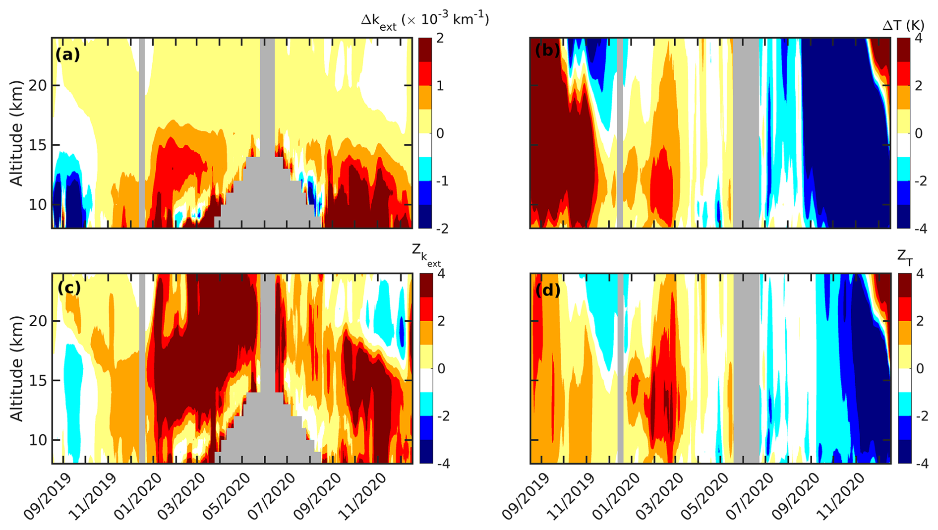
Figure 2 The daily vertical anomaly (Δ) in OMPS (a) k_ext at 745 nm and (b) temperature and the standardized anomaly (Z) in (c) k_ext at 745 nm and (d) temperature averaged between a latitude of −60 and −90° from September 2019 to December 2020 are shown. The gray-shaded region corresponds to no data. The ticks on the x axis mark the middle of each month. The black diamond in each plot marks the Black Summer event.

The vertical profiles of the anomaly and standardized anomaly (Z) in k_ext and temperature are shown in Fig. 2. Significant aerosol loading is observed (as shown in Fig. 2a) between altitudes of 10 and 25 km from January to June 2020. The continuous increase in $Z_{k_{\mathrm{ext}}}$ from January 2020, to an even higher altitude (Fig. 2c), is attributed to a self-lofting mechanism (Khaykin et al., 2020). Like Fig. 1, the positive anomaly in k_ext in the lower stratosphere from October to December 2020 surpassed the anomaly observed during early 2020. The major type of aerosol emitted during the Black Summer was organic carbon (Yu et al., 2021), which is hydrophilic in nature. Thus, the increased k_ext could have been due to the exposure of these aerosols to low temperatures during winter, when the condensation of water vapor would have resulted in the growth of the aerosols, thereby further increasing their size and light extinction. In addition, the transport of more bushfire aerosols from middle- to high-latitude regions could be another cause of the observed increase in Δk_ext. The descending pattern observed in Z_kext (Fig. 2c) from August to December 2020 could have been due to the descent of the mesospheric air, as explained by Kessenich et al. (2023).

OMPS does not provide information about aerosols during polar winter due to the lack of solar radiation, as seen in Figs. 1 and 2 (gray-shaded regions). Hence, the total attenuated backscatter (β) at 532 nm measured by CALIPSO for grids classified as “No Cloud (NC)” at temperatures above the equilibrium temperature of NAT particles (T_NAT) is chosen to study the influence of the Black Summer event on lower-stratospheric aerosol in the high-latitude region during the Austral winter of 2020 (Fig. S3). As the total attenuated backscatter is above T_NAT, it could correspond to the lower-stratospheric aerosols, thus excluding the influence of sub-visible PSCs or PSCs. From May to mid-June 2020, the total attenuated backscatter varied between $\mathrm{1.6}\times {\mathrm{10}}^{-\mathrm{4}}$ and $\mathrm{1.8}\times {\mathrm{10}}^{-\mathrm{4}}$ (km⁻¹ Sr⁻¹), which is more than 1 standard deviation with respect to the background mean (Fig. S3). After mid-June 2020, the total attenuated backscatter value returned to its background level.

These observations reveal high aerosol loading in the lower stratosphere of the high latitudes after the Black Summer event. This can increase the surface area available for heterogeneous chemical reactions and, potentially, modify the stratospheric chemistry itself. For a comprehensive understanding of the impact of the Black Summer event on the PSC dynamics, we explore the changes in the key constituent gases of PSCs in the next section.

4.2 Enhanced HNO₃ and H₂O in the lower stratosphere

The anomalies in MLS HNO₃ and H₂O mixing ratios along with their corresponding standardized anomalies averaged between latitudes of −60 and −90° are shown in Fig. 3. An elevated HNO₃ mixing ratio was observed between 20 and 30 km altitude from February 2020, and this value had peaked at 1.5 ppb over the background value by April 2020 (Fig. 3a). This surge exceeded 2 standard deviations and remained significant until June 2020 at an altitude of 20 km (Fig. 3c). Similarly, an increase in the H₂O mixing ratio was observed at slightly lower altitudes (between 15 and 20 km) from mid-January 2020 (Fig. 3b) and exceeded more than 1 standard deviation (the cause of this anomalous increase is discussed in Sect. 4.3). As both HNO₃ and H₂O are principal constituents of PSCs (Tabazadeh et al., 1994; Voigt et al., 2000; Höpfner et al., 2006; Tritscher et al., 2021), the near-simultaneous decrease in them along with k_ext (Figs. 2a and S3) during Austral winter suggests that these species condensed on the bushfire aerosols and were, thus, likely converted into PSCs.

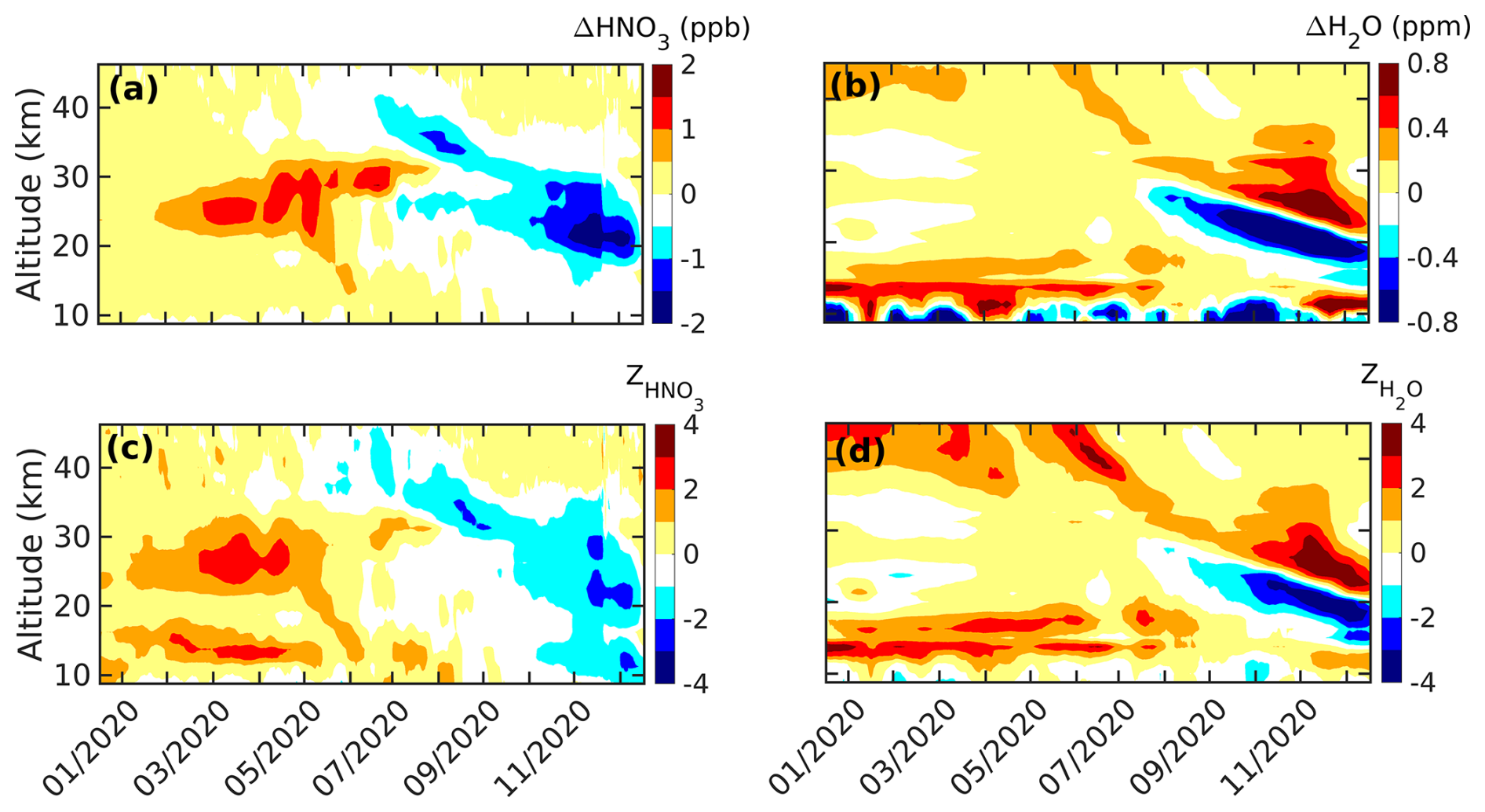
Figure 3 The anomaly in the (a) HNO₃ and (b) H₂O mixing ratios and the standardized anomaly in the (c) HNO₃ and (d) H₂O mixing ratios, averaged between latitudes of −60 and −90° during 2020. The ticks on the x axis mark the middle of each month.

Unlike HNO₃, abundant water vapor is detected in the upper stratosphere (above 40 km) (Fig. 3b and d) from January to April 2020. As there is no evidence that the smoke plume from the Black Summer event reached such altitudes, we believe that the moist upper stratosphere is not associated with the aforementioned event. The upper-stratospheric water vapor is produced through the oxidation of methane (CH₄; Brewer, 1949; Fueglistaler et al., 2009) and directly injected from the tropical tropopause layer through deep convection (Schoeberl et al., 2018). This water vapor is further transported from low to high latitudes through a deep branch (present at the upper and middle stratosphere) and a shallow branch (present just above tropopause) of the Brewer–Dobson circulation (Butchart, 2014). The descent of water vapor from the upper stratosphere to the lower stratosphere during 2020 (shown in Fig. 3b) suggests that this water vapor was carried by the deep branch of the Brewer–Dobson circulation and resulted in a strong positive H₂O anomaly from September to December 2020 at altitudes of 30 to 25 km. A strong negative anomaly in both HNO₃ and H₂O can be observed below this layer during early 2020, which could be due to the prolonged polar vortex during this period separating the middle- and high-latitude air masses, thereby preventing further mixing (Rieger et al., 2021; Klekociuk et al., 2022; Santee et al., 2022; Yook et al., 2022). To understand whether the cause of these anomalies was due to dynamic (i.e., due to change in transportation) or chemical (i.e., due to chemical reaction) processes, a tracer–tracer correlation analysis was carried out, the results of which are discussed in the next section.

4.3 Tracer–tracer correlation analysis

The tracer–tracer correlation analysis technique is used to diagnose whether a change in the atmospheric gas concentration is driven by chemical reactions or transportation (such as convection or advection). The idea behind this technique is that chemically active and long-lived trace (i.e., chemically inert) gas should exhibit the same order of change if the cause is transport-related (e.g., Müller et al., 1996, 1997); however, if a chemically active gas increases/decreases with no change in long-lived trace gas, the change is attributed to chemical reaction. In this technique, a linear regression between a long-lived trace gas and a chemically active gas is performed for both species during the background period. A deviation of the data corresponding to the period of interest from the regression line indicates the chemical production of the chemically active gases. Likewise, an alignment with the regression line indicates a transport-related source of the chemically active gases. For our analysis, hydrofluoric acid (HF) was chosen as the long-lived trace gas, as it is chemically inert in the stratosphere (Wang et al., 2023).

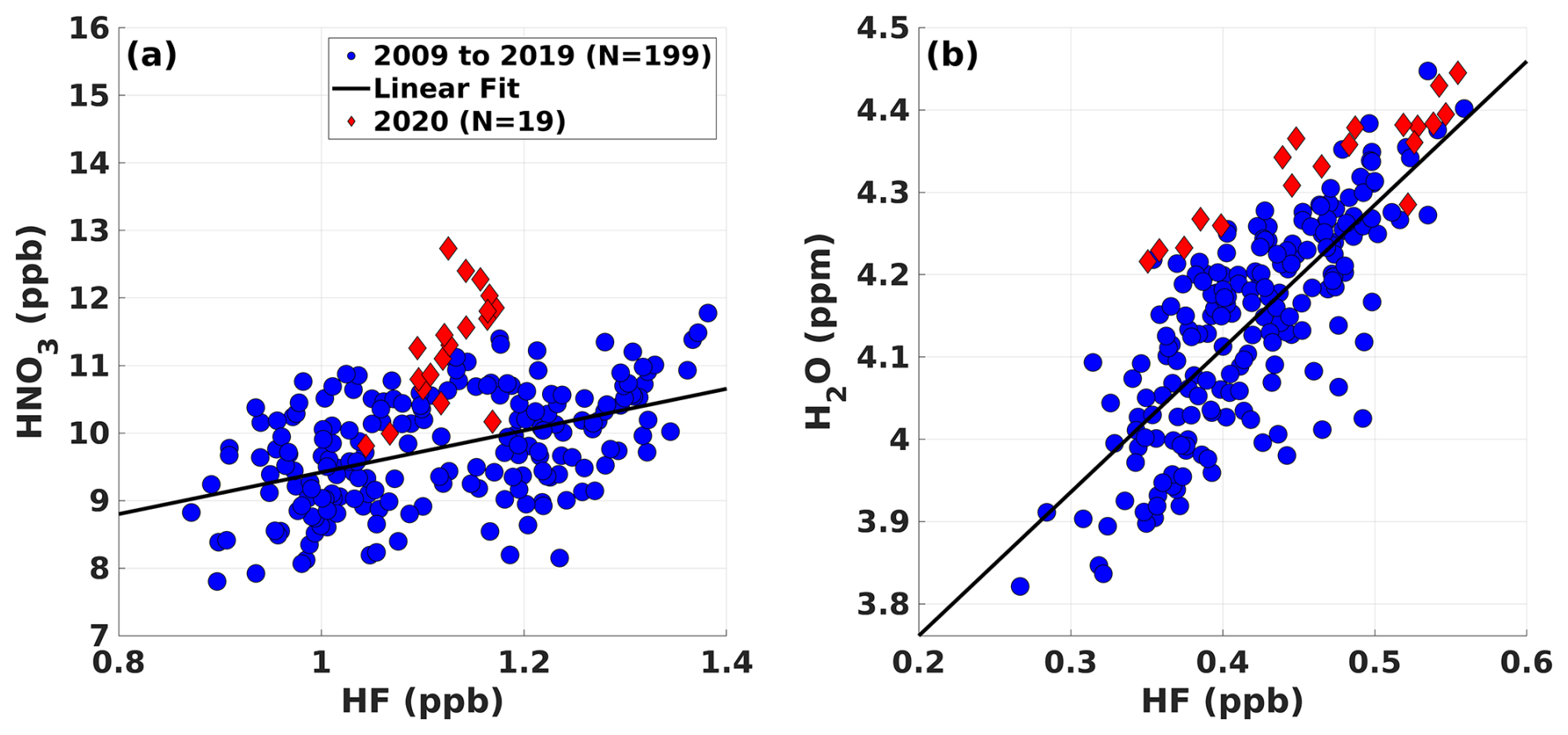
Figure 4 Tracer–tracer correlation of ACE-FTS (a) HNO₃ vs. HF at an altitude of 25 km and of (b) H₂O vs. HF at an altitude of 17 km within the latitude range of −60 to −90°. The blue circles correspond to March in the period from 2009 to 2019, the red diamonds correspond to March in 2020, and the solid black line is a regression line. Here, N is the number of data points used for regression analysis for both panels.

The ACE-FTS-obtained HF is regressed against HNO₃ and H₂O at altitudes of 25 and 17 km, respectively, during March 2009–2019 (Fig. 4). The results suggested that the HNO₃ was produced via a chemical process, as the data corresponding to March 2020 (red diamond in Fig. 4a) deviate greatly from the regression line (black line). In contrast, increased H₂O is transport-related, as the data are close to the regression line (Fig. 4b), and this species was likely carried to the lower stratosphere by smoke plumes from the Black Summer event (Schwartz et al., 2020). The production of HNO₃ in the lower stratosphere is governed by the heterogeneous chemical reactions of dinitrogen pentoxide (N₂O₅) hydrolysis, which can be written as follows (Zhang et al., 1995):

$$\begin{array}{}\text{(R1)}& {\mathrm{N}}_{\mathrm{2}}{\mathrm{O}}_{\mathrm{5}}+{\mathrm{H}}_{\mathrm{2}}\mathrm{O}\to \mathrm{2}{\mathrm{HNO}}_{\mathrm{3}}.\end{array}$$

To confirm the involvement of the N₂O₅ hydrolysis process, H₂O, N₂O₅, and HNO₃ from ACE-FTS and k_ext at 745 nm from OMPS at a 25 km altitude at high latitude (−60 to −90°) from February to May 2020 are analyzed and shown in Fig. 5. A coinciding depletion in ACE-FTS N₂O₅ at an altitude of 25 km can be observed during the same period (Fig. 5c). Thus, we have performed a similar tracer–tracer correlation analysis for N₂O₅ (Fig. S2). The result indicates that N₂O₅ is chemically depleted in the lower stratosphere, suggesting the possible role of the N₂O₅ hydrolysis process. In general, the stratospheric background aerosols provide a surface for H₂O to condense upon, and gas-phase N₂O₅ reacts with it to form HNO₃.

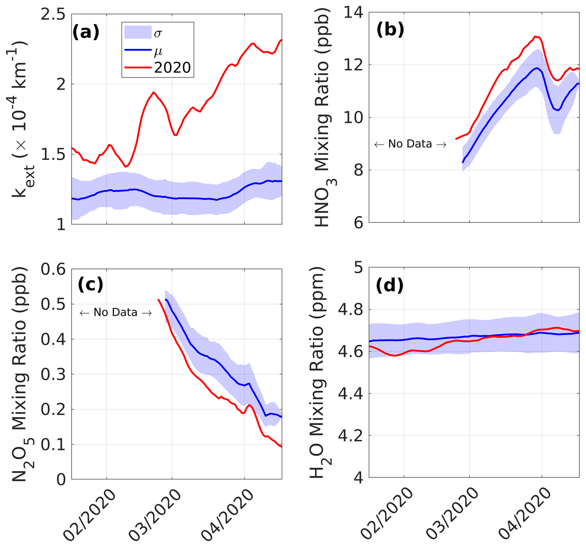
Figure 5 OMPS-obtained (a) k_ext at 745 nm and ACE-FTS-obtained (b) HNO₃, (c) N₂O₅, and (d) H₂O mixing ratios at an altitude of 25 km averaged over the latitude band from −60 to −90°. Here, σ represents the standard deviation with respect to the background mean μ estimated for the 2009–2019 period. The ticks on the x axis mark the middle of each month.

The background mean k_ext value remains at ∼ $\mathrm{1.25}\times {\mathrm{10}}^{-\mathrm{4}}$ km⁻¹ between February and May (Fig. 5a). However, beginning in early 2020, k_ext gradually increased to peak at $\mathrm{2.4}\times {\mathrm{10}}^{-\mathrm{4}}$ km⁻¹ by April 2020. This increasing trend in k_ext could be attributed to the coupled effect of the transportation of even more bushfire aerosols from middle to high latitudes as days passed and to aerosol ages, as the bushfire aerosols mixed with stratospheric sulfate aerosols resulted in an increased size and extinction coefficient (Li et al., 2021; Ohneiser et al., 2022). The simultaneous production and depletion of HNO₃ and N₂O₅ exceeded the respective standard deviations and substantiated that HNO₃ is produced through N₂O₅ hydrolysis (Fig. 5b and c).

During Austral winter, due to the continued lack of solar radiation, the temperature of the polar region decreases to less than 195 K; this results in the condensation of trace gases onto stratospheric aerosols, forming PSCs. The near-simultaneous decrease in aerosol loading, HNO₃, and H₂O in the lower stratosphere (as discussed in Sect. 4.2) during the early winter of 2020 suggests that these changes possibly affected PSC formation. A comprehensive investigation of PSC dynamics was carried out using CALIPSO measurements and is discussed in the next section.

4.4 Impact of the Black Summer event on PSCs during 2020

We first investigated the onset of PSCs during 2020 with respect to the previous years. The onset of each type of PSC is determined for the years 2009 to 2020 (excluding 2015) and provided in the Supplement (Table S1). The onset is defined as the first instance when each PSC type is detected by CALIPSO. We did not observe the early onset of any PSCs during 2020. However, the onset of STS PSCs occurred on 26 May 2020, which is slightly later than the usual onset period of these PSCs. It should be noted that there are sub-visible PSCs which are not detected by CALIPSO, as those PSCs' optical properties are below the CALIPSO detection threshold (Lambert et al., 2012, 2016). Hence, the actual onset could be 1 to 3 d earlier than these dates. The sub-visible PSCs are often studied via the depletion of HNO₃ during early winter. We used MLS HNO₃ to check whether there was early/late depletion in HNO₃ leading to an early/late onset of PSCs during 2020 at an altitude of 20 km (Fig. S4). Figure S4 shows that the depletion of HNO₃ usually occurs during or after the middle of May every year at an altitude of 20 km and that the pattern remained unchanged for 2020, suggesting no sign of the early HNO₃ depletion. This observational evidence from MLS HNO₃ and CALIPSO PSC data suggests that there is neither the early depletion of HNO₃ nor the early onset of PSCs.

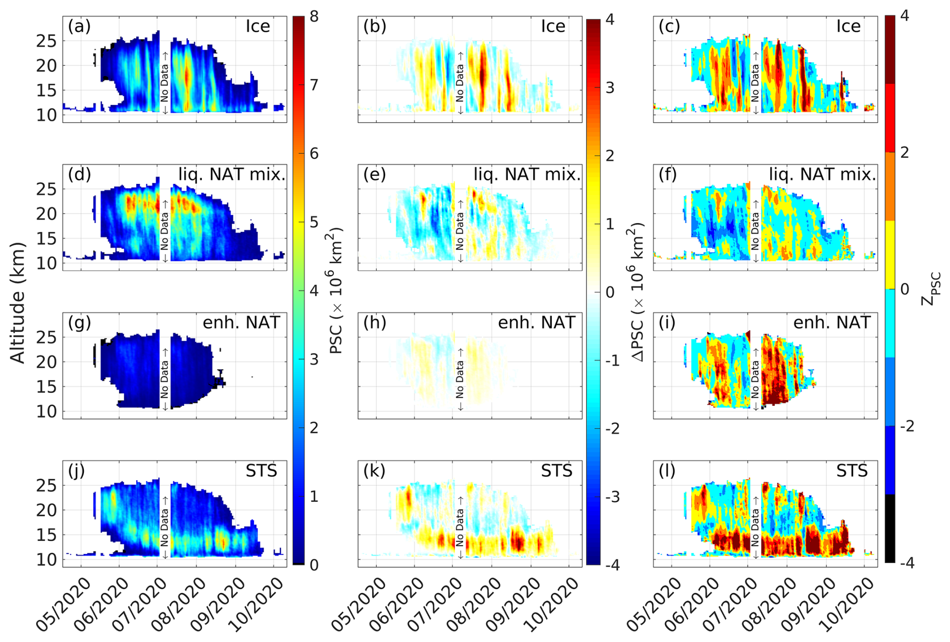
Figure 6 CALIPSO Antarctic PSC areal coverage (left column, panels a, d, g, and j), anomaly (middle column, panels b, e, h, and k), and standardized anomaly (right column, panels c, f, i, and l) for the year 2020. Here, “liq. NAT mix.” is a liquid–NAT mixture and “enh. NAT” is enhanced NAT.

The Antarctic PSC areal coverage for each PSC type for the year 2020 and the corresponding anomalies and standardized anomalies are estimated (as described in Sect. 3.2) and are shown in Fig. 6. The anomaly in the total PSC areal coverage is shown in Fig. S5. CALIPSO detected PSCs from late May onwards (Fig. 6). Around the same time, the depletion of HNO₃ is also observed via MLS (Fig. 3). A peak positive anomaly of up to 4×10⁶ km² is exhibited by ice PSCs at an altitude of between 15 and 20 km during the second week of August 2020. Followed by ice PSCs, the supercooled ternary solution (STS) PSCs exhibited a high positive anomaly, which peaked at up to 3.5×10⁶ km² at an altitude of between 12 and 15 km during early September 2020 (Carslaw et al., 1994; Molina et al., 1993; Ravishankara and Hanson, 1996). Similarly, an increase in enhanced NAT PSC areal coverage is observed, but its contribution to the total PSC areal coverage is negligible. It is evident from Fig. 6b, h, and k that the positive anomalies in the areal coverage of PSCs like ice, STS, and enhanced NAT PSCs exceeded 3 standard deviations with respect to the background mean. Furthermore, during June and July 2020, the areal coverage of liquid–NAT mixture PSCs decreased significantly, leading to a negative anomaly of up to 2.5×10⁶ km², which is more than 2 standard deviations from the background mean (Fig. 6e and f). During the same period, a significant increase in ice PSC areal coverage of up to 2×10⁶ km² was observed, exceeding 2 standard deviations (Fig. 6b and c).

Interannual variabilities in polar vortex and polar stratospheric clouds

In general, PSCs exhibit a strong interannual variation owing to the polar vortex dynamics, such as vortex temperature and area. Hence, to understand the association of the polar vortex variability with the observed PSCs anomalies, the statistics, such as the minimum, maximum, mean, and standard deviation of the PSC volume, for each PSC type observed from 2009 to 2020 (excluding the year 2015) and their relationship with polar vortex dynamics are studied in detail and shown in Fig. 7. Here, the polar vortex is defined as the region enclosed by the 32 PVU (potential vorticity unit) potential vorticity contour, following the definition from Kondragunta et al. (2005). The vortex area is quantified as the total area within this defined region, while the vortex temperature represents the mean temperature over the same area. The potential vorticity and temperature are taken from the ERA5 operational analysis dataset.

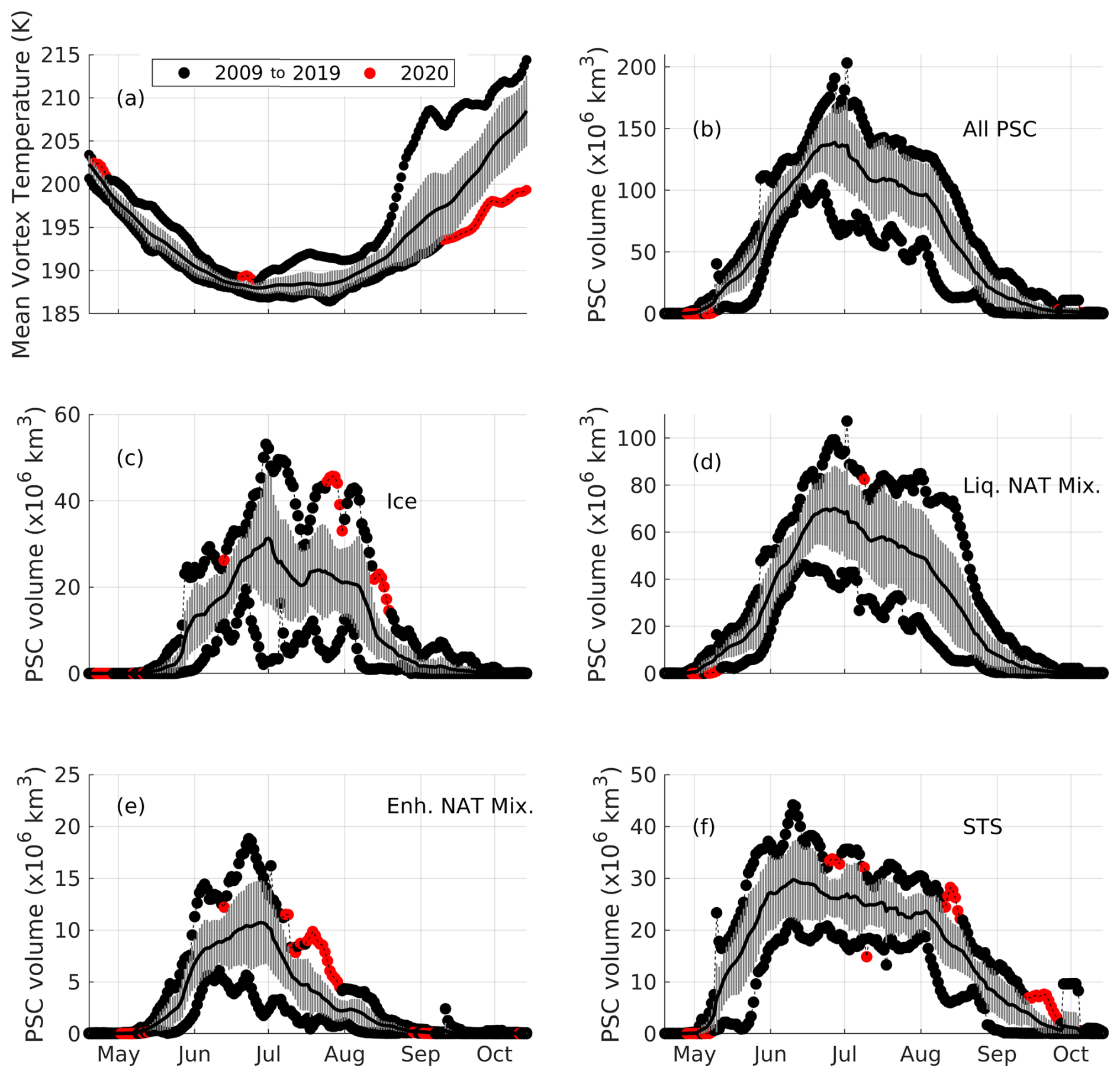
Figure 7 Time series of the CALIPSO-obtained PSC volume over the Antarctic from 2009 to 2020 (excluding 2015) are shown. Panel (a) shows the mean vortex temperature obtained from the ERA5 operational analysis at a potential temperature of 450 K, while panels (b), (c), (d), (e), and (f) show the volume of all PSCs, ice PSCs, Liq. NAT Mix. PSCs, Enh. NAT Mix PSCs, and STS PSCs, respectively. The solid black line represents the mean PSC volume, and the vertical lines represent the standard deviation. The daily maximum and minimum PSC volumes are color-coded according to the period in which they occurred. The red-filled circles mark the anomalous high/low value in PSC volume and mean vortex temperature during 2020, and black-filled circles mark the period from 2009 to 2019.

During early May and June of 2020, the mean vortex temperature was the highest compared to the background period (from 2009 to 2019, excluding the year 2015) (Fig. 7a). In contrast, the mean vortex temperatures for the remaining months up to September 2020 were neither the warmest nor the coldest. However, after September 2020, the mean vortex temperature dropped to its lowest levels (ranging from 194 to 200 K), which can be attributed to the prolonged vortex period and ozone depletion. Owing to this colder environment, STS PSCs continued to appear (even after September 2020), resulting in the highest STS PSC volume with respect to the background period. However, this colder condition was not sufficient to affect the formation of other PSC types (i.e., notable positive anomaly) after September 2020 (Figs. 6 and 7). In terms of total PSC volume (i.e., a sum of the volume of total PSC types), no anomalous behavior in the total PSC volume was observed, in keeping with the results reported by Li et al. (2024). However, upon investigation of the individual PSC volume, we found that ice, enhanced NAT, and STS PSCs exhibited anomalously high volumes for a certain period during 2020, exceeding 1 standard deviation (Fig. 6c, i, and l) as well as the recorded decadal high value (Fig. 7c, e, and f; marked with red-filled circles). The periods from 8 to 14 August 2020 and from 27 August to 9 September 2020 recorded the highest ice PSC volume among the years from 2009 to 2020, reaching up to 45×10⁶ km³ and 22×10⁶ km³, respectively. Similarly, the year 2020 recorded the highest enhanced NAT PSC volume of up to 12×10⁶ km³ during the period from 21 to 30 July 2020. For the STS PSCs, the second week of July and the last week of August 2020 recorded the highest PSC volume. However, the liquid–NAT mixture PSC volume did not exhibit significant anomalies relative to other PSC types. As the magnitude of the PSC volume also depends on the polar vortex dynamics, we investigated the polar vortex area and mean temperature for the year 2020 and compared these values with the background period.

Early May and early June of 2020 were the warmest periods in the background period (Fig. S3a). However, on most of the days from late June to early August of 2020, the Antarctic polar vortex area was recorded to be the highest, ranging between 23×10⁶ km² and 32×10⁶ km². In contrast, this period was not the coldest, as revealed by the mean vortex temperature. We checked the role of this increased polar vortex area during 2020 with respect to the increased PSCs by investigating the vortex occurrence frequency anomaly at a potential temperature level of 450 K and the PSC volume from June to August 2020. For this purpose, a positive anomaly in the vortex occurrence frequency greater than 1 standard deviation with respect to the background period (the single-hatched region in Fig. 8) and a negative anomaly greater than 1 standard deviation (the cross-hatched region in Fig. 8) are overlaid on the monthly PSC volume anomaly.

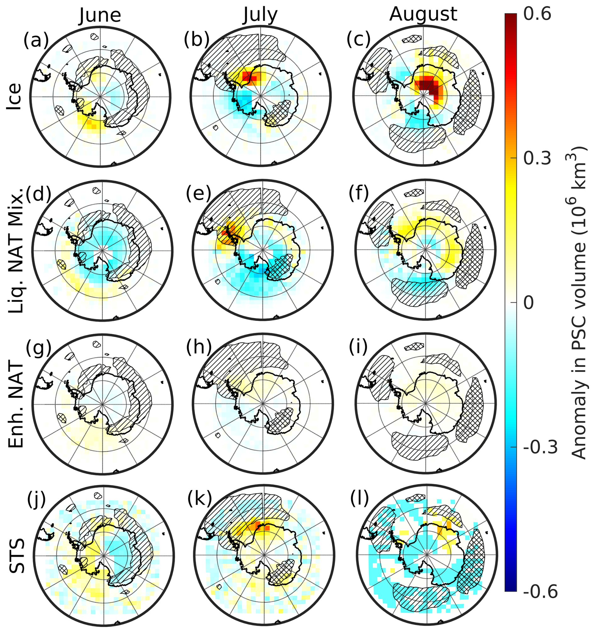
Figure 8 Monthly mean PSC volume anomalies for June (left column), July (middle column), and August (right column) are shown. Single-hatched regions indicate a positive anomaly in polar vortex occurrence frequency exceeding 1 standard deviation, while cross-hatched regions indicate a negative anomaly exceeding 1 standard deviation.

During June 2020, the vortex occurrence frequency exceeded 1 standard deviation over the eastern Antarctic and northeastern regions (marked with single hatching in Fig. 8, left column), indicating a significant expansion of the polar vortex in these areas. However, no positive anomalies in any PSC types were observed over the same region, suggesting that the increased vortex area during June 2020 did not influence PSC formation (Fig. 8, left column). In July 2020, the polar vortex shifted off the South Pole toward the Antarctic Peninsula, resulting in a significant positive anomaly in vortex occurrence frequency over the northwestern region (marked with single hatching in Fig. 8, middle column) and a negative anomaly over the southeastern region (marked with cross-hatching in Fig. 8, middle column). Over the Antarctic Peninsula, a positive anomaly in the liquid–NAT mixture PSC volume slightly overlapped with this stretched vortex area, while no other PSC types exhibited anomalous behavior (Fig. 8, middle column). By August 2020, the vortex expanded further, stretching toward the Antarctic Peninsula, whereas it contracted over the eastern Antarctic region (Fig. 8, right column). Although a significant increase in PSC volume was observed during this month, particularly for ice and liquid–NAT mixtures, these PSCs remained confined close to the South Pole. This again suggests that the increased polar vortex area did not influence PSC formation or contribute to the observed positive anomalies in PSC volume. As discussed earlier in Fig. 7, except for liquid–NAT mixture PSCs, the volume of other PSCs exhibited anomalous behavior during certain periods of 2020. To further understand the observed anomalies, we compared the mean vortex temperature and PSC volumes from 2020 with those from previous years (2009–2019). For this comparison, we specifically selected time periods during which notable anomalies were observed in each PSC type during 2020. These include the ice PSC volume from 8 to 14 August (Fig. 9a) and from 27 August to 9 September (Fig. 9b), the enhanced NAT mixture PSC volume from 21 to 30 July (Fig. 9c), and the STS PSC volume from 23 to 30 August (Fig. 9d). These periods were chosen because at least one type of PSC recorded its highest volume in 2020 compared to any year between 2009 and 2019 (Fig. 7, red-filled circles). The mean vortex temperature from 8 to 14 August 2020 was ∼ 188 K, which was considerably warmer than previous years (such as 2011, 2016, 2017, 2018, and 2019). Despite this relatively warm condition, the mean ice PSC volume was observed to be 46×10⁶ km³ (Fig. 9a), which was significantly higher than in previous years. Similarly, from 27 August to 9 September, the mean vortex temperature was ∼ 191 K. Once again, it was not the coldest period when compared to the years from 2009 to 2019. Nonetheless, the mean ice PSC volume peaked at 22.5×10⁶ km³, which was 2-fold higher than the previously recorded values. Similar observations were made in the case of the enhanced NAT mixture and STS PSC volumes (Fig. 9c and d), for which significant increases in their respective PSC volume were observed despite the vortex temperature being comparable to the previous years.

This analysis indicates that the increased PSC areal coverage and volume cannot be attributed to vortex dynamics, such as variations in vortex area or temperature. Instead, we attribute these anomalously high PSC areal coverage and volume values to the intrusion of bushfire aerosols from the Black Summer event. In summary, the stratospheric intrusion of bushfire aerosols resulted in the increased production of HNO₃ via enhancement of the N₂O₅ hydrolysis process while also increasing HNO₃-containing PSCs, such as STS and enhanced NAT mixture PSCs. However, despite the relatively high availability of HNO₃ during 2020, no significant anomaly in the liquid–NAT mixture PSCs was observed. One possible explanation for this observation could be the rapid conversation of NAT particles into ice PSCs, as NAT can serve as an efficient nucleus for ice formation (Hoyle et al., 2013). To verify this hypothesis, we performed Lagrangian backward-trajectory analysis of the ice and liquid–NAT mixture PSCs to study their respective formation pathways as discussed Sect. 3.3; the results of this analysis are discussed in the next section.

4.5 Formation pathways of liquid–NAT mixture and ice PSCs

In this section, the formation pathways of ice and liquid–NAT mixture PSCs are presented in the form of case studies. Here, we discuss a few case studies that are considered representative of each formation pathway of liquid–NAT mixture and ice PSCs. A total of five case studies are discussed: three cases for liquid–NAT mixture PSCs and two cases for ice PSCs. The liquid–NAT mixture and ice PSCs are selected according to the selection criteria discussed in Sect. 3.3, and backward trajectories are calculated using the CLaMS trajectory module with meteorological parameters obtained from the ERA5 operational analysis dataset. Liquid–NAT mixture PSCs can form via either an ice-free nucleation process or an ice-assisted nucleation process. Evidence of the former process is discussed using case no. 1, whereas evidence of the latter process is discussed using case nos. 2 to 3. Similarly, evidence of the formation of ice through a NAT-assisted formation pathway and a NAT-free formation pathway is discussed using case nos. 4 and 5, respectively.

4.5.1 Ice-free nucleation of liquid–NAT mixture PSCs

In this section, we discuss case no. 1, in which NC (No Cloud) precedes the liquid–NAT mixture along the backward trajectory. In this case, there is no evidence of the formation of ice in either the CALIPSO observations or based on the presence of conditions conducive to ice formation, suggesting the possibility of the ice-free nucleation of liquid–NAT mixture PSCs.

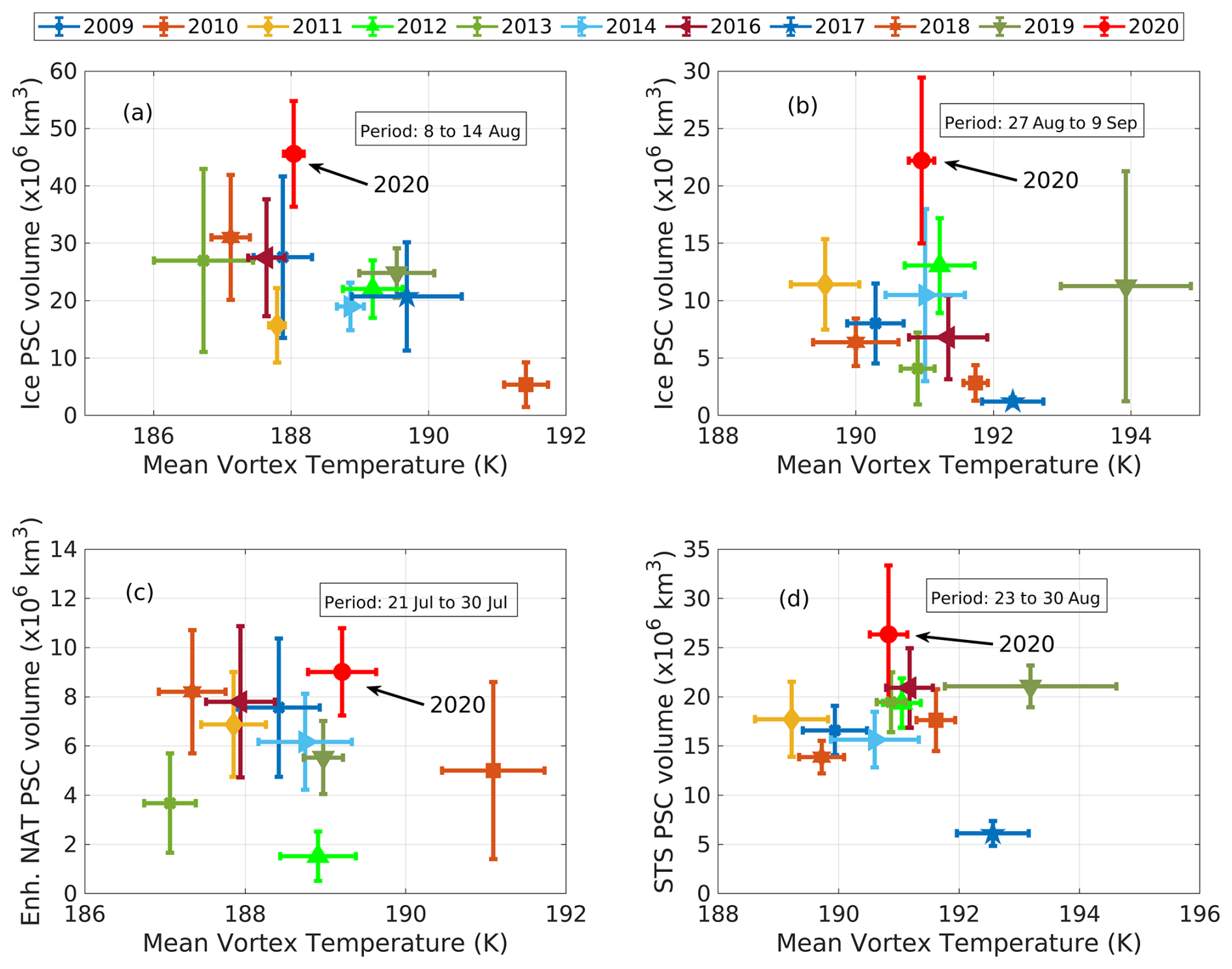
Figure 9 The relationships of the mean vortex temperature with ice (a, b), enh. NAT (c), and STS (d) PSC volume are shown. The center of each marker represents the mean value, while the vertical and horizontal lines indicate 1 standard deviation of the daily PSC volume and mean vortex temperature for each period (shown using a rectangle in each panel), respectively. The black arrows in each panel point to the data corresponding to the year 2020.

Case no. 1: NC precedes a liquid–NAT mixture PSC

At 18:00 UTC on 10 July 2020, CALIPSO detected a liquid–NAT mixture PSC at a latitude of −69.1° and longitude of 99.15°, with a potential temperature of 484 K. This observation is marked by a yellow diamond in Fig. 10a, and the corresponding CALIPSO scan track is shown as a solid gray line; the CALIPSO PSC orbit curtain plot is shown in Fig. S7a. The dashed black line in Fig. 10a represents the calculated 48 h backward trajectory of this PSC, with the color indicating the temperature history of the air parcel in T_ice coordinates, i.e., ambient temperature (T) − the frost point (T_ice). The temperature (T) is obtained from the ERA5 operational analysis, and T_ice is estimated using the ERA5 pressure and the mean MLS H₂O mixing ratio found along the trajectory, following Marti and Mauersberger (1993).

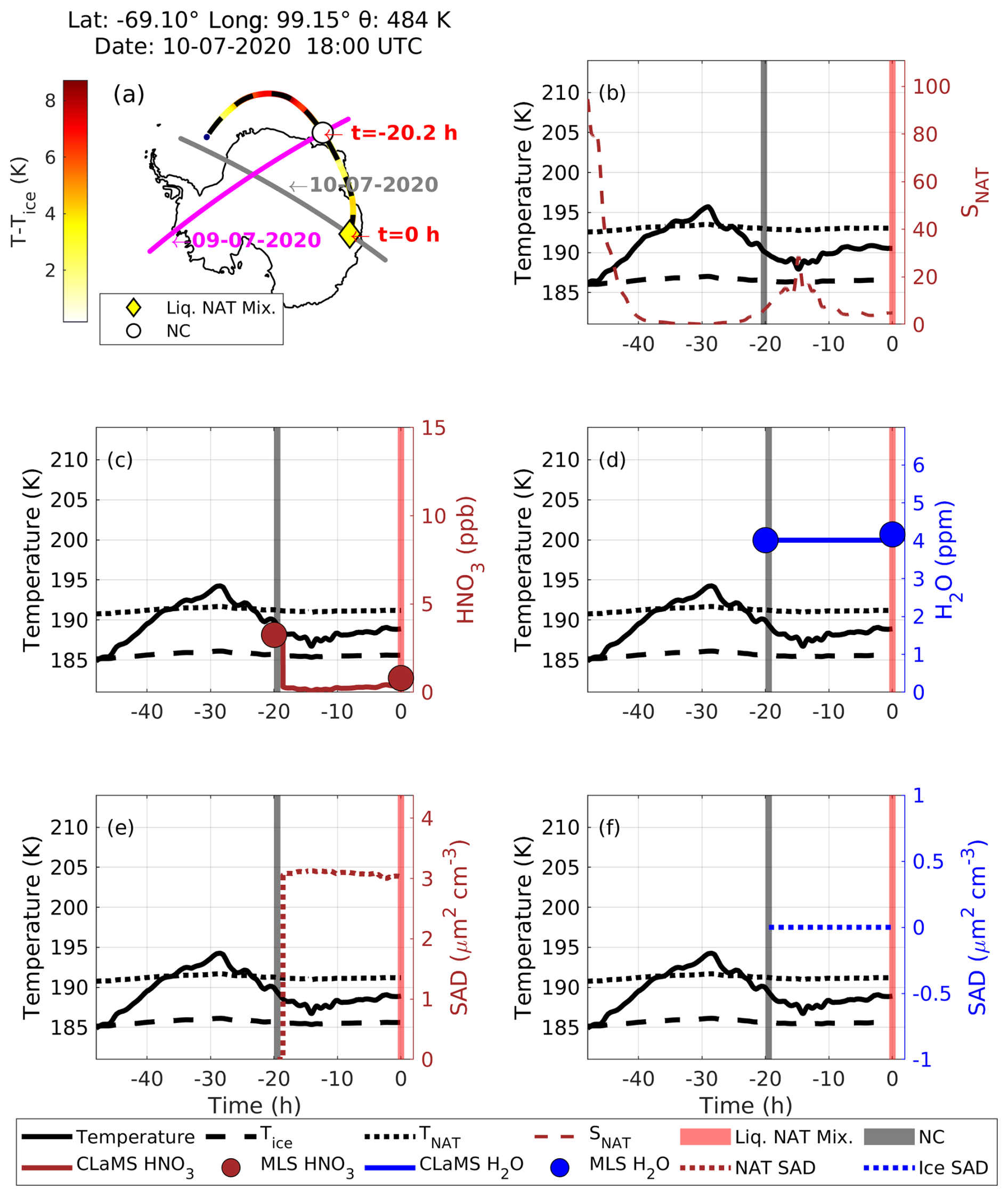
Figure 10 (a) The Lagrangian backward trajectory for a 48 h period starting at time t=0 h (corresponding to 18:00 UTC on 10 July 2020). Here, the dashed black line is the backward trajectory, while the color along this trajectory is the temperature at the T–T_ice coordinate. The yellow diamond represents the observed liquid–NAT mixture PSC from the CALIPSO scan track (solid gray line) corresponding to 10 July 2020, and the corresponding CALIPSO PSC orbit curtain plot is shown in Fig. S7b. The complete coordinate information for this liquid–NAT mixture PSC is given in the panel heading. The white circle represents the observed “No Cloud (NC)” at time $t=-\mathrm{20.2}$ h from the CALIPSO scan track (solid magenta line) corresponding to 9 July 2020. Panel (b) presents the saturation ratio over NAT (S_NAT) (dashed brown line), and vertical bars mark the liquid–NAT mixture PSC (red) and NC (gray). In panel (c), the brown circle marks the MLS HNO₃, and the solid brown line represents the CLaMS HNO₃. In panel (d), the blue circle marks the MLS H₂O, and the solid blue line represents the CLaMS H₂O. Panel (e) presents the NAT surface area density (SAD) (dotted brown line), whereas panel (f) shows the ice SAD (dotted blue line).

The backward trajectory revealed that CALIPSO observed “No Cloud (NC)” along this trajectory 20.2 h earlier (at $t=-\mathrm{20.2}$ h), on 9 July 2020, marked by a white circle in Fig. 10a. The temperature history shows that the temperature did not decrease below T_ice between these two observations, indicating that the conditions were not conducive to ice formation. At the time of the NC observation, the temperature was ∼ 189 K, which is 2 K below the NAT temperature (T_NAT). During this time, MLS-observed gas-phase HNO₃ and H₂O mixing ratios were 3.5 ppb and 4 ppm, respectively (Fig. 10c and d). Using these as initial conditions, a CLaMS box model run was performed from $t=-\mathrm{20.2}$ to 0 h, simulating the evolution from NC to a liquid–NAT mixture PSC. After 20.2 h, the MLS HNO₃ decreased from 3.5 to 0.5 ppb, with no significant change in MLS H₂O. Figure 10c and d show that the CLaMS-modeled uptake of HNO₃ and H₂O agrees well with the MLS observations. Furthermore, the CLaMS box model run indicates that the NAT surface area density (SAD) increased to nearly 3 µm² cm⁻³ (shown in Fig. 10e), while the ice SAD remained at 0 µm² cm⁻³, supporting that no ice formation occurred before the observation of the liquid–NAT mixture PSC. During the transition from NC to the liquid–NAT mixture PSC, the saturation ratio over NAT stayed well below 30, further supporting the absence of ice involvement in the formation of the liquid–NAT mixture PSC (Fig. 10b; Luo et al., 2003; Voigt et al., 2005). As the liquid–NAT mixture PSC represents the mixture of liquid STS and solid NAT, it should be noted that a STS PSC should have formed between this transition and, specifically, before the formation of NAT. From this detailed case study of ice-free nucleation of the liquid–NAT mixture PSC discussed above, it is evident that the temperature of the trajectories did not decreased below T_ice and that S_NAT remained below 30, thus confirming no ice involvement during the liquid–NAT mixture PSC formation. Another example of an STS PSC preceding the observation of a liquid–NAT mixture PSC along the backward trajectory is shown in Fig. S8. Even in this case, the conditions are not conducive to ice formation between the observation of an STS PSC and a liquid–NAT mixture PSC, confirming that the NAT formed without ice. For brevity, further details of this case are not discussed here.

4.5.2 Ice-assisted nucleation of liquid–NAT mixture PSCs

Here, two cases are discussed: case no. 2 and case no. 3. In the former case, the direct CALIPSO observation of ice preceding a liquid–NAT mixture PSC along the trajectory is presented. In the latter case, CALIPSO-observed NC precedes a liquid–NAT mixture PSC, but the conditions conducive to ice formation are found before the formation of the liquid–NAT mixture PSC, indicating the possibility of an ice-assisted nucleation process.

Case no. 2: an ice PSC precedes a liquid–NAT mixture PSC

In this case, an ice PSC appeared along the backward trajectory before the appearance of a liquid–NAT mixture PSC, indicating the nucleation of NAT on the pre-existing ice PSC. At 23:00 UTC on 5 July 2020, CALIPSO detected a liquid–NAT mixture PSC (yellow diamond in Fig. 11a) at a latitude of −66.89°, longitude of 25.89°, and potential temperature of 510 K. The CALIPSO PSC orbit curtain plot for this observation is shown in Fig. S9. Before this, CALIPSO observed an ice PSC along this trajectory at $t=-\mathrm{43}$ h on 4 July 2020 (blue star in Fig. 11a).

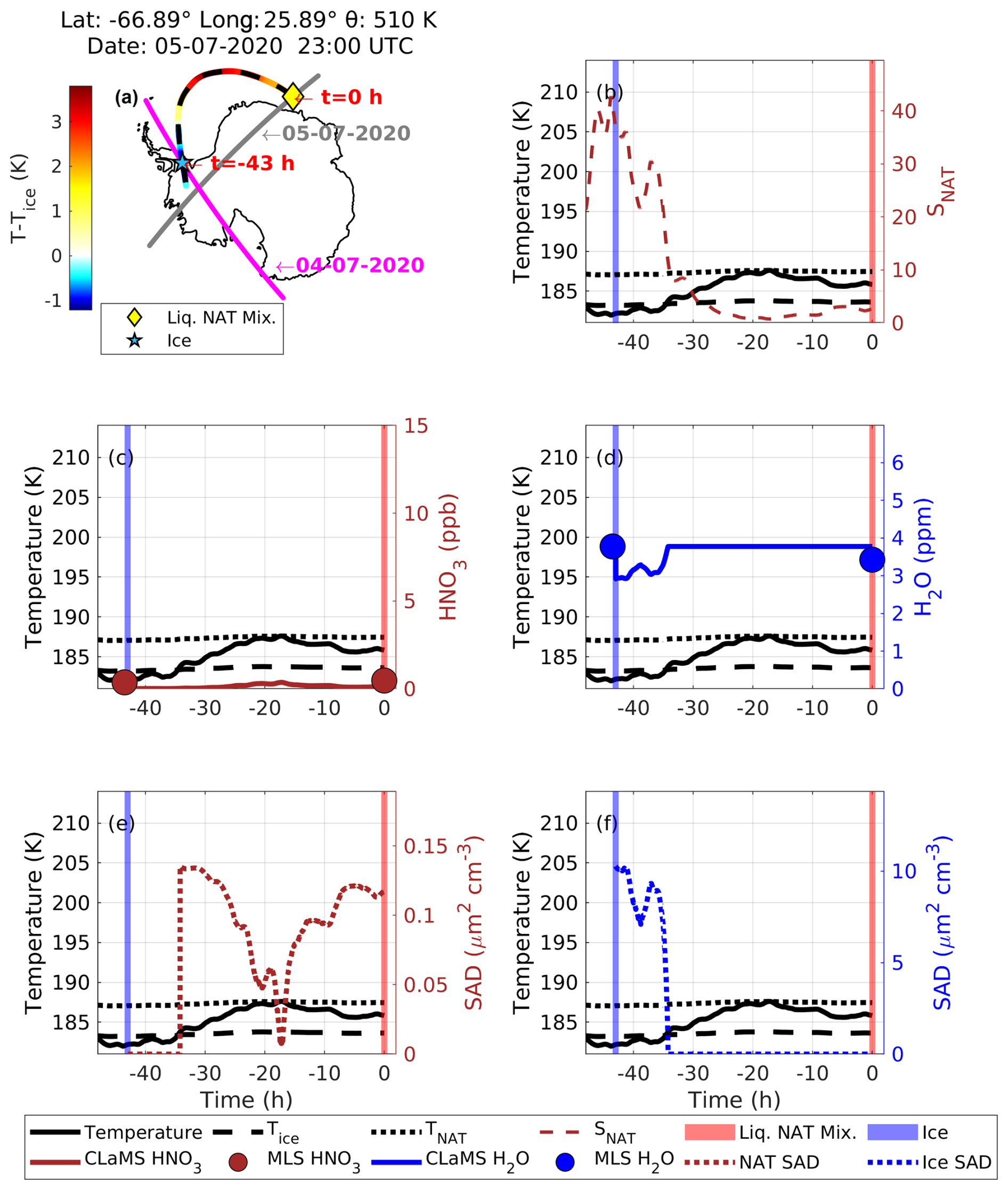
Figure 11 Similar to Fig. 10 but for case no. 2, in which ice preceded the liquid–NAT mixture PSC along the Lagrangian backward trajectory.

At the time of ice detection, the temperature was approximately 181.5 K, which is 1.5 K below T_ice. During this time, MLS-observed gas-phase HNO₃ and H₂O mixing ratios were 0.37 ppb and 3.9 ppm, respectively. Furthermore, at this time, according to the CLaMS box model run, ice SAD was ∼ 10 µm² cm⁻³ and NAT SAD was 0 µm² cm⁻³ (Fig. 11e and f). After this, the temperature gradually increased, exceeding T_ice, which decreased the ice SAD to 0 µm² cm⁻³ and increased NAT SAD to 0.14 µm² cm⁻³, possibly due to the nucleation of NAT particles on this ice. During the transition from ice to the liquid–NAT mixture PSC, the maximum S_NAT was observed to be 43 at $t=-\mathrm{43}$ h. The MLS-observed HNO₃ increased from 0.37 to 0.47 ppb, whereas H₂O decreased from 3.7 to 3.4 ppb. It should be noted that these changes in HNO₃ and H₂O are within MLS measurement uncertainty.

Case no. 3: NC precedes a liquid–NAT mixture PSC

In this case, NC is observed before the observation of a liquid–NAT mixture PSC. However, the temperature along the trajectory decreased well below the ice formation temperature (i.e., below T_ice−1.5 K), indicating the possible formation of ice and, thus, the nucleation of NAT on this ice PSC.

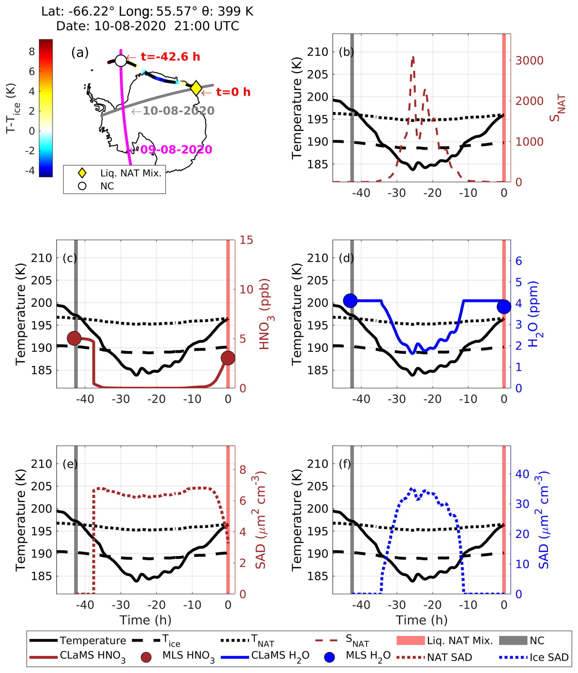
Figure 12 Similar to Fig. 10 but for case no. 3, in which NC preceded a liquid–NAT mixture PSC along the Lagrangian backward trajectory.

At 21:00 UTC on 10 August 2020, CALIPSO detected a liquid–NAT mixture PSC (indicated by a yellow diamond in Fig. 12a) at a latitude of −66.22°, longitude of 55.57°, and potential temperature of 399 K. The CALIPSO PSC orbit curtain plot for this observation is shown in Fig. S10. Before this observation, CALIPSO observed NC along this trajectory at $t=-\mathrm{42.6}$ h on 9 August 2020. During that period, the temperature was around 197 K, which is 0.4 K above the T_NAT, and MLS-measured gas-phase HNO₃ and H₂O mixing ratios were 5 ppb and 4.1 ppm, respectively. These conditions were not favorable for the formation of any type of PSC. Approximately 4.6 h later (i.e., at $t=-\mathrm{38}$ h), the temperature decreased below T_NAT (by 3 K), which likely promoted the formation of NAT, as supported by the CLaMS box model run, with the NAT SAD reaching up to 6 µm² cm⁻³ (Fig. 12e). No ice formation occurred at this stage, as the temperature remained above T_ice. However, the temperature continued to decline, reaching T_ice at $t=-\mathrm{35}$ h, at which point ice began to appear in the CLaMS model, as indicated by the ice SAD (Fig. 12f).

As the temperature fell to 184 K, which is 5 K below T_ice, the ice SAD peaked at 35 µm² cm⁻³, suggesting that these ice particles may have nucleated on the previously formed NAT. By this time, the CLaMS model shows that HNO₃ had been depleted from an initial value of 5 ppb to a value of 0.002 ppb, while H₂O decreased from 4.1 to 1.6 ppm. Additionally, S_NAT peaked at ∼ 3000 (Fig. 12b). Unlike in case nos. 1 and 2, in which ice was not involved in NAT formation, a significant change in H₂O was observed in this instance due to the formation of ice. Subsequently, the temperature began to increase gradually and reached a value above T_ice at $t=-\mathrm{11}$ h, resulting in an ice SAD of 0 µm² cm⁻³. At this point, all condensed H₂O evaporated back into the gas phase, returning to the initial level of 4.1 ppm. In contrast, the gas-phase HNO₃ remained below 0.1 ppb. The temperature continued to increase, and CALIPSO detected a liquid–NAT mixture PSC at t=0 h; during this time MLS observed HNO₃ levels of 3.1 ppb, while the CLaMS-modeled HNO₃ was 3.5 ppb. Throughout this process, MLS HNO₃ decreased from 5 to 3.1 ppb, leaving 1.9 ppb in the condensed phase.

In summary, when the temperature was above T_NAT, no cloud was observed by CALIPSO. As the temperature decreased below T_NAT−3 K, NAT formed first, followed by ice nucleation when the temperature decreased below T_ice. As the temperature increased, additional NAT particles nucleated on the existing ice. Although the CLaMS box model suggests the presence of ice between $t=-\mathrm{35}$ and −11 h, there were no co-located CALIPSO observations along the trajectory to verify the presence of an ice PSC. However, we identified another backward trajectory related to the CALIPSO-detected liquid–NAT mixture PSC at a potential temperature of 388 K (which is 11 K lower than the current trajectory of 399 K), as shown in Fig. S11. The temperature fluctuations along this trajectory are similar to those in case no. 4, in which a co-located CALIPSO observation of an ice PSC was recorded at time $t=-\mathrm{29.4}$ h. A similar case, in which an STS PSC precedes a liquid–NAT mixture PSC but in which the temperature along the trajectory decreased below the T_ice, creating conditions favorable for ice formation, is presented in Fig. S12, along with the CLaMS box model run. Given the similarities between this case and case no. 3, which has been described above, we have not provided a detailed analysis of the case in which STS PSC precedes a liquid–NAT mixture PSC.

In these two cases of an ice-assisted nucleation process of liquid–NAT mixture PSCs, the temperature decreased below T_ice and S_NAT increased more than 30. Therefore, the extent to which the temperature decreased below T_ice and the extent to which the S_NAT increased along the trajectories from the instant of observation of an NC/STS/ice to the instant of the liquid–NAT mixture PSC observation can act as proxies to determine whether the liquid–NAT mixture PSC is formed via an ice-assisted or ice-free nucleation process.

4.5.3 Validation of the uptake of HNO₃ and H₂O observed during liquid–NAT mixture formation

During the formation of the liquid–NAT mixture, changes in the gas-phase concentrations of MLS HNO₃ and H₂O were observed, as previously discussed. We used the CLaMS microphysical box model to simulate the formation of the liquid–NAT mixture based on the backward trajectories and then modeled the uptake of HNO₃ and H₂O. These results were validated against the observed uptake values from MLS, as shown in Fig. 13. This result includes both the ice-assisted and ice-free nucleation of the liquid–NAT mixture.

A strong correlation is found between the MLS-observed change in HNO₃ (ΔHNO₃) and the CLaMS-modeled change in HNO₃, with a correlation coefficient (R) of 0.64 and a coefficient of determination (R²) of 0.4096 (Fig. 13a). The intercept of −2.72 suggests that the CLaMS model overestimates the HNO₃ condensation during NAT formation. This could be due to a possible cold bias in temperature from the ERA5 operational analysis that is used in this study. Furthermore, significant HNO₃ uptake of up to 12 ppb, as observed by MLS, occurred when NC preceded the observation of the liquid–NAT mixture PSC along the trajectory (indicated by the white circle in Fig. 13a). However, a relatively low HNO₃ uptake is observed for cases in which an STS PSC preceded the liquid–NAT mixture (marked by the green circle in Fig. 13a). It is important to note that ice may have formed during the transition from NC/STS to the liquid–NAT mixture, as discussed in case no. 3. Furthermore, in most cases where ice preceded the liquid–NAT mixture along the trajectory, a positive change in MLS ΔHNO₃ is observed; however, more detailed studies are required to understand these scenarios further.

In the case of H₂O uptake, a weak correlation is found between MLS ΔH₂O and CLaMS ΔH₂O, with an R of 0.23 and an R² of 0.0529 (Fig. 13b). In addition to the cold temperature bias in the ERA5 operational analysis, this low correlation is also attributed to the fact that the initialized H₂O at the beginning of the trajectory only changes in the CLaMS model if ice forms during liquid–NAT mixture formation, resulting in most of the CLaMS ΔH₂O values remaining at zero. However, there are a few instances in which changes in H₂O are observed in both CLaMS and MLS, potentially indicating ice-assisted formation of the liquid–NAT mixture. Furthermore, for simplicity, other chemical reactions (e.g., N₂O₅ hydrolysis and HCl null cycles) that involve H₂O are not considered in the CLaMS box model run, as discussed in Sect. 3.4. Hence, even if such reactions occur and deplete/produce H₂O in a real atmosphere, the CLaMS box model run does not account for them. This simplified box model run likely contributes to the weak correlation between H₂O values from CLaMS and MLS observations. A similar reasoning could apply to HNO₃; however, as the HNO₃ depletion is primarily driven by NAT formation, the omission of other chemical reactions in the simplified box model does not significantly affect the correlation between HNO₃ values from CLaMS and MLS.

4.5.4 Relative percentage contribution of the liquid–NAT mixture formation pathway

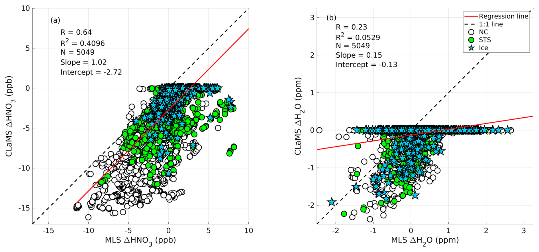
Figure 13 Panel (a) shows a scatterplot of MLS-observed change (Δ) in HNO₃ (ppb) against the CLaMS modeled change in HNO₃ (ppb). Panel (b) shows a scatterplot of MLS-observed change (Δ) in H₂O (ppm) against the CLaMS modeled change in H₂O (ppm). The dashed line represents a 1:1 fit, and the solid red line represents the linear regression line. Here, R is the correlation coefficient, R² is the correlation of determination, and N is the total number of data points used. Each marker corresponds to the PSC type preceding the liquid–NAT mixture along the backward trajectory: white-filled circles represent NC, green-filled circles represent STS, and blue-filled pentagrams represent ice.

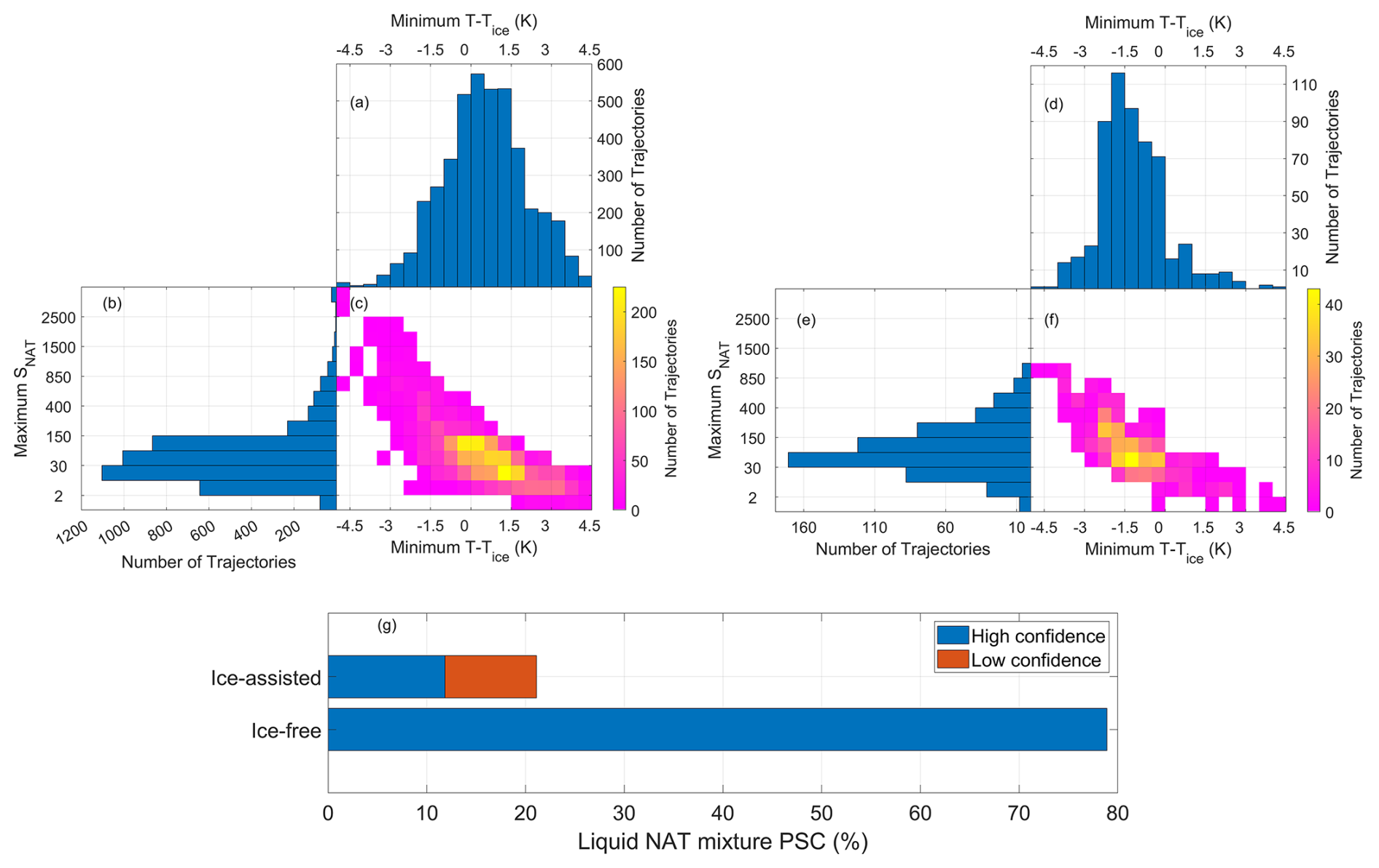
Figure 14 Histograms and joint histograms of the minimum T–T_ice and the maximum S_NAT (saturation ratio over NAT) along the trajectories are shown. Panels (a)–(c) correspond to the backward trajectories in which NC/STS preceded the liquid–NAT mixture CALIPSO observation. Panels (d)–(f) are similar to panels (a)–(c) but for the case of ice preceding the liquid–NAT mixture. Panel (g) shows the percentage of the liquid–NAT mixture formed through ice-assisted and ice-free nucleation processes.

As discussed in case nos. 1 and 2, the presence of NC/STS preceding the liquid–NAT mixture along the trajectories does not exclude the involvement of ice in the formation of the liquid–NAT mixture. It is possible that ice could have formed before the observation of the liquid–NAT mixture if the temperature decreased well below T_ice and reached a state of high NAT supersaturation. Therefore, the extent of the temperature decrease below T_ice and the extent of the corresponding increase in S_NAT along the trajectories, from the time of NC/STS observation to the formation of the liquid–NAT mixture, can serve as indicators of whether the liquid–NAT mixture formed through ice-assisted or ice-free nucleation. To investigate this, we created two sets of histograms. Figure 14a, b, and c show the histograms of minimum T–T_ice and maximum S_NAT along the trajectories for cases in which NC/STS preceded the liquid–NAT mixture. Figure 14d, e, and f show similar histograms for cases in which ice preceded the liquid–NAT mixture. In all cases, the minimum T–T_ice and maximum S_NAT were only considered from the time of NC/STS (for Fig. 14a–c) or ice (for Fig. 14d–f) observation until the liquid–NAT mixture formed.

For cases in which NC/STS preceded the liquid–NAT mixture, the histogram of minimum T–T_ice (Fig. 14a) shows that most trajectories experienced T–T_ice values between −0.5 and 1.5 K, with the highest peak between 0 and 0.5 K. Similarly, the histogram of maximum S_NAT (Fig. 14b) shows that most trajectories had S_NAT values ranging from 15 to 150, with a peak between 15 and 30. A cluster of trajectories (represented by yellow to orange grids) is visible in the joint histogram (Fig. 14c) within this range. With respect to the formation of ice along these trajectories, the temperature should have reached at least −1.5 K for the heterogeneous nucleation of ice, and a high S_NAT of >500 (Luo et al., 2003) should have occurred for the nucleation of NAT on these ice particles. As neither condition is observed and, thus, conditions are not conducive to ice formation, it is highly likely that the liquid–NAT mixture formed via an ice-free nucleation process. Case no. 1, which was discussed earlier, belongs to this category. In addition, when the minimum T–T_ice decreased below −1.5 K, the air parcels reached a high supersaturation, with S_NAT values exceedingly reaching values as high as 500. Case no. 3, which was also discussed earlier, belongs to this category. Under these conditions, the formation of ice and the subsequent nucleation of NAT on this ice is likely, indicating that the liquid–NAT mixture may have formed via ice-assisted nucleation. This observation aligns with the previous findings by Luo et al. (2003) on NAT formation over ice under high-supersaturation conditions.

For cases in which ice preceded the liquid–NAT mixture along the trajectory, the histogram of minimum T–T_ice (Fig. 14d) shows that most trajectories experienced T–T_ice values between −2 and −1 K, with the highest peak between −2 and −1.5 K. Similarly, the histogram of maximum S_NAT (Fig. 14e) shows that most trajectories had S_NAT values ranging from 15 to 150; however, for this case, the highest peak occurs between 30–70, instead of 15–30 (as observed a previous case). A cluster of trajectories (represented by yellow to orange grids) is visible in the joint histogram (Fig. 14f) within this range. Case no. 2, which was discussed earlier, belongs to this category, as ice preceded the liquid–NAT mixture.

From these two sets of histograms, an apparent shift in minimum T–T_ice is evident between cases in which NC/STS preceded the liquid–NAT mixture (peak between 0 and 0.5 K) and cases in which ice preceded the liquid–NAT mixture (peak between −2 and −1.5 K). In contrast, only a subtle shift is observed in maximum S_NAT. Therefore, to determine whether ice was involved in the formation of the liquid–NAT mixture, we primarily rely on the minimum T–T_ice reached by each trajectory, rather than the maximum S_NAT.

Cases in which ice preceded liquid–NAT mixture were classified with high confidence as ice-assisted nucleation of liquid–NAT mixture. We specify that these cases were classified with “high confidence” because we have CALIPSO observations of the presence of ice along the trajectory, similar to case no. 2. Moreover, for cases in which NC/STS preceded the liquid–NAT mixture, if the temperature along the trajectories decreased to less than −1.5 K, we classified the case as ice-assisted nucleation of a liquid–NAT mixture, although with low confidence. These cases are classified with low confidence because ice formation is not directly observed by CALIPSO, but ice was possibly formed as the temperature decreased 1.5 K below T_ice. For the cases in which NC/STS preceded the liquid–NAT mixture, if the temperature along the trajectories did not decrease to less than −1.5 K, we classified them with high confidence as the ice-free nucleation of liquid–NAT mixture. The final retrieved relative percentage of the liquid–NAT mixture formation pathway is shown in Fig. 14g. The figure shows that 79 % of the liquid–NAT mixture (corresponding to 2996 backward trajectories) is formed via an ice-free formation process with high confidence. Almost 12 % and 9 % of the liquid–NAT mixture (corresponding to 796 backward trajectories) formed via an ice-assisted formation process with high and low confidence, respectively.

4.5.5 NAT-assisted ice formation

In the case of the NAT-assisted ice formation pathway, evidence of a direct CALIPSO observation of liquid–NAT mixture along the backward-trajectory ice PSC is given in Fig. S13. For brevity, this case is not discussed in detail here. Instead, another example of NAT-assisted ice formation pathways in which “NC” precedes an ice PSC is elaborated upon in detail through case no. 4.

Case 4: NC precedes an ice PSC

In this case, NC is observed before the observation of ice. At 18:00 UTC on 19 June 2020, CALIPSO detected ice (blue star symbol in Fig. 15a) at a latitude of −80.96°, longitude of 6.00°, and potential temperature of 451 K. Before this, CALIPSO had observed NC along this trajectory at $t=-\mathrm{37.6}$ h on 18 June 2020. The CALIPSO PSC orbit curtain plots for these observations are shown in Fig. S14. During the observation of NC, the temperature was around 192.5 K, which is 1 K above T_NAT (Fig. 15b), and MLS measured gas-phase HNO₃ and H₂O mixing ratios of 2 ppb and 3.7 ppm, respectively (Fig. 15c and d). As the temperature was above T_NAT, there was no possibility of the formation of PSCs at this time. Approximately 14.6 h later (i.e., at time $t=-\mathrm{13}$ h), as the temperature decreased below T_NAT, a strong depletion in CLaMS HNO₃ was observed, while the CLaMS H₂O mixing ratio remained unchanged. Concurrently, NAT SAD increased to ∼ 2.7 µm² cm⁻³ (Fig. 15e). At $t=-\mathrm{18}$ h, ice SAD started increasing gradually as the temperature reached T_ice (Fig. 15f), and it reached a peak value of ∼ 20 µm² cm⁻³. This suggests the nucleation of ice on the NAT particles.

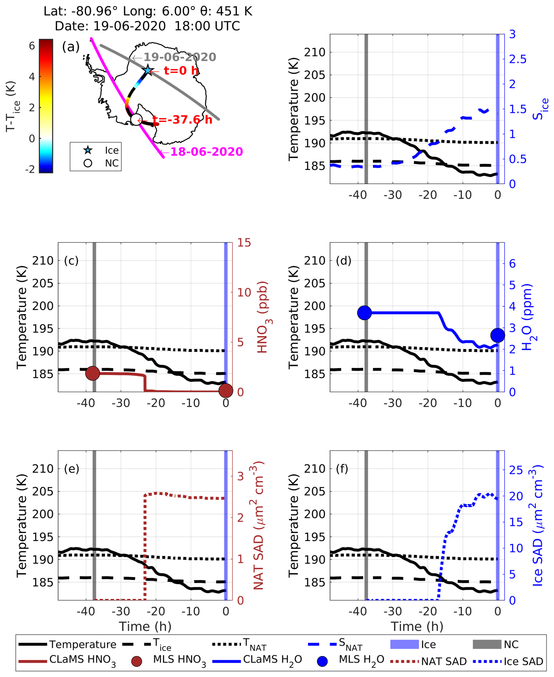
Figure 15 Same as Fig. 10 but for case no. 4, in which ice nucleation on NAT is shown.

4.5.6 NAT-free ice formation

In this section, we discuss case no. 5, in which the NAT-free ice nucleation process leads to ice formation.

Case 5: NC precedes an ice PSC

In this case, NC is observed before the observation of ice along its backward trajectory. At 18:00 UTC on 19 June 2020, CALIPSO detected ice (blue star symbol in Fig. 16a) at a latitude of −80.41°, longitude of 359.56°, and potential temperature of 497 K. Before this, CALIPSO had observed NC along this trajectory at $t=-\mathrm{37.6}$ h on 18 June 2020. The CALIPSO PSC orbit curtain plots for these observations are shown in Fig. S15. There are notable similarities between case no. 4 and case no. 5. In both cases, the latitude, longitude, and temperature histories of the observed ice PSCs and the preceding NC observations along the backward trajectory are almost identical. However, the ice PSC is located at a potential temperature of 497 K in case no. 5 (Fig. 17a), whereas the PSC in case no. 4 is at a relatively lower potential temperature of 451 K (Fig. 16a). Despite having similar temperature histories, ice formed via nucleation on NAT in case no. 4, whereas ice formed without NAT in case no. 5. A key difference between the two cases is the availability of gas-phase HNO₃. For case no. 5, the MLS HNO₃ mixing ratio at the CALIPSO NC observation time is 0.6 ppb (denitrified scenario), which is 1.4 ppb lower than that of case no. 4. Hence, compared to case no. 4, relatively low MLS HNO₃ is observed for case no. 5 when the temperature was above T_NAT. The CLaMS box model for case no. 5 shows no NAT formation along the trajectory, with the NAT SAD remaining at 0 µm² cm⁻³ (Fig. 16e), whereas the NAT SAD increases to 2.7 µm² cm⁻³ for case no. 4 (Fig. 16e). This is because there is not enough gas-phase HNO₃ (with just 0.6 ppb) to form NAT in case no. 5, as it might have already been removed due to the growth of NAT to a large size, leading to denitrification before the observation of NC itself. In both cases, ice forms as the temperature drops below T_ice, with the ice SAD reaching ∼ 23 µm² cm⁻³ in case no. 5, which is 3 µm² cm⁻³ higher than in case no. 4 (Fig. 16f). Furthermore, during ice formation, the maximum S_ice is ∼ 1.5 in case no. 4, compared to a high-supersaturation S_ice of 1.8 in case no. 5 (Fig. 16b). As ice can form through a homogeneous nucleation process at S_ice>1.5, the temperature needs to be 3 K below T_ice. However, for this case, the temperature is just 2 K below T_ice, suggesting the heterogeneous nucleation of ice without NAT. One possibility could be that STS with the inclusion of foreign nuclei could have resulted in the formation of ice in this case. Another example in which STS precedes an ice PSC but in which liquid–NAT mixture was not formed, as modeled by CLaMS, is given in Fig. S16. As the bushfire aerosols entered the lower stratosphere in the high-latitude region, as shown in Figs. 1 and 2, it is highly likely that the STS contained these aerosols along with other foreign nuclei. In short, under the denitrified scenario, in which there is the insufficient availability of gas-phase HNO₃, ice can form via a NAT-free nucleation process. Based on PSC measurement using lidar aboard HALO, Voigt et al. (2018) observed ice PSCs with a bimodal distribution of the particle depolarization ratio over the Arctic region on 22 January 2016. Lagrangian backward-trajectory analysis revealed that the ice with a high depolarization ratio is preceded by NAT, based on CALIPSO measurements. Furthermore, ice with a low depolarization ratio is preceded by STS. Hence, to investigate ice formation via NAT-free and NAT-assisted nucleation process cases, we analyzed the depolarization ratio of ice, as discussed in the next section.

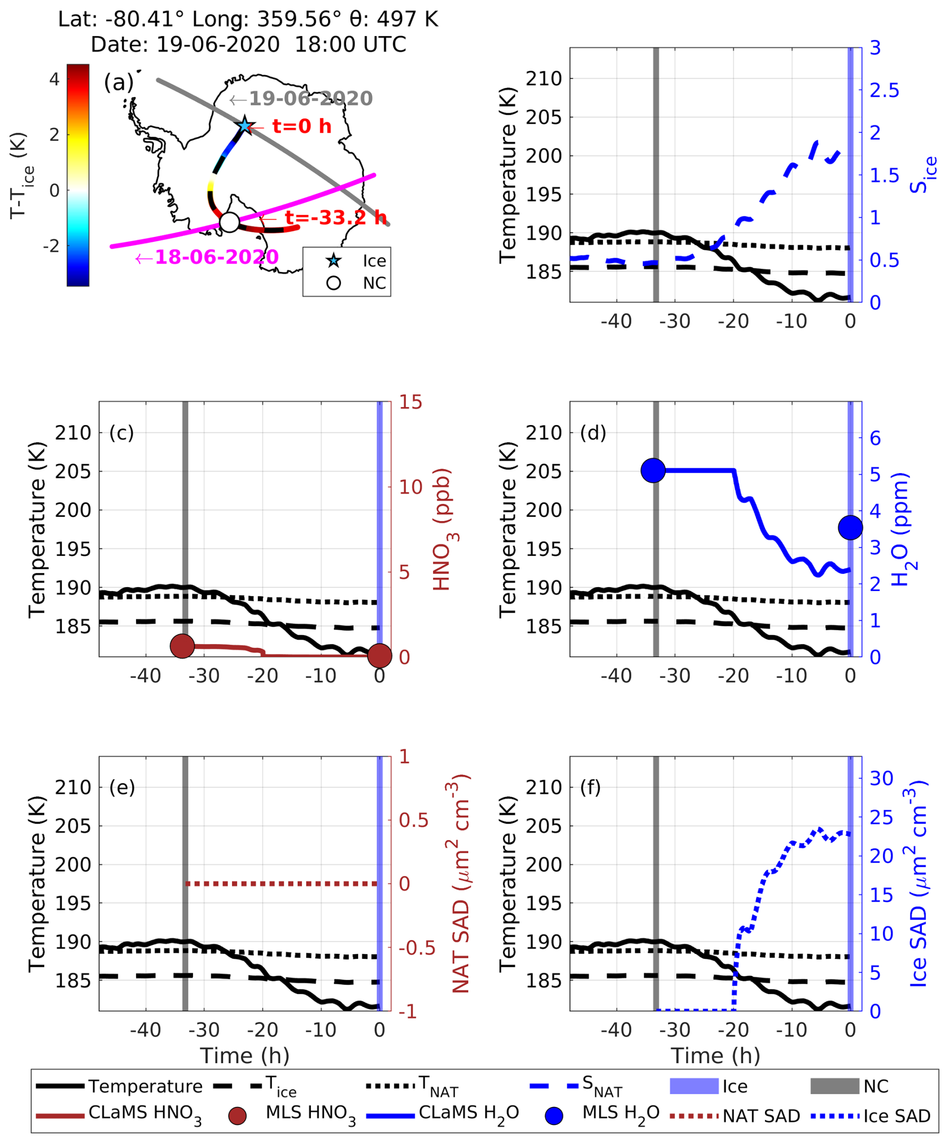
Figure 16 Same as Fig. 10 but for case no. 5, in which ice nucleated without NAT.

4.5.7 Bimodal distribution of the depolarization ratio of ice PSCs

The depolarization ratios of ice preceded by a liquid–NAT mixture and STS along the backward trajectories are analyzed, with the corresponding probability densities shown in Fig. 17. As discussed through the case studies, after the CALIPSO observation of STS, it is possible that a liquid–NAT mixture formed as the temperature decreased and that these NAT particles acted as nuclei for ice formation. Therefore, the probability density of the depolarization ratio for the STS case may reflect not only the formation of ice on STS but also ice nucleated on NAT. The probability densities of the depolarization ratio for ice preceded by a liquid–NAT mixture (solid red line in Fig. 17a) peak at 0.35. In contrast, the probability density for ice preceded by STS (solid black line in Fig. 17a) shows a bimodal distribution, with a high depolarization mode peaking at 0.26 and a low depolarization mode peaking at 0.07. This observation of a bimodal distribution of the depolarization ratio is similar to the findings reported by Voigt et al. (2018). This bimodal distribution suggests that, under certain conditions, ice nucleates on NAT/STS, contributing to the mixed depolarization signal. Using the example in Fig. S16 and case no. 5, it is shown that, under denitrified conditions, the ice can form via a NAT-free formation pathway.

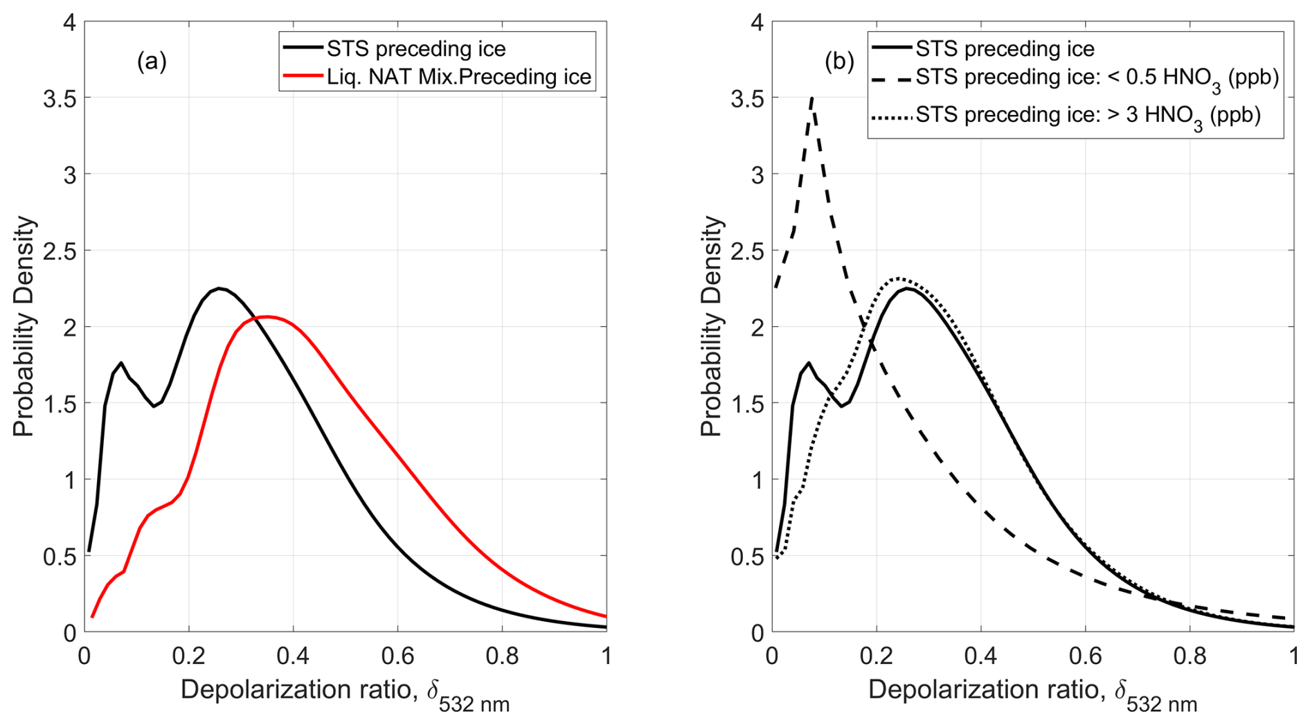
Figure 17 (a) The probability densities of the depolarization ratio of ice preceded by STS (solid black line) and liquid–NAT mixture (solid red line) are shown. Panel (b) presents the decomposition of ice preceded by STS based on MLS HNO₃ mixing ratios: <0.5 ppb (dashed line) and >3 ppb (dotted line).

Therefore, we chose ice PSCs that are preceded by STS under the denitrified condition of MLS HNO₃<0.5 ppb (i.e., during the observation of STS along the backward trajectory of ice, the MLS HNO₃ should be <0.5 ppb) and under the normal condition of MLS HNO₃>3.0 ppb. Figure 17b shows the depolarization ratio of ice preceded by STS, distinguishing between cases under a denitrified scenario (MLS HNO₃<0.5 ppb, dashed black line) and under normal conditions (MLS HNO₃>3 ppb, dotted black line). These threshold values of 0.5 and 3 ppb are chosen because they effectively separate the bimodal distribution into two clearly distinguishable modes. The lower threshold (0.5 ppb) captures conditions under which denitrification is significant and, thus, NAT is less likely to form, leading to ice nucleation directly on STS with foreign nuclei inclusion. On the other hand, the higher threshold (3 ppb) represents conditions under which sufficient HNO₃ is available for NAT formation, supporting ice nucleation via NAT-assisted processes. These thresholds help differentiate the distinct nucleation pathways reflected in the depolarization ratio distributions. The low-HNO₃ case shows a more pronounced peak at lower depolarization values (∼ 0.076), whereas the high-HNO₃ case follows a distribution more similar to the overall STS case (with a higher depolarization peak near 0.26). This suggests the potential influence of the availability of gas-phase HNO₃ on the ice nucleation processes. Under normal gas-phase HNO₃ conditions with respect to availability, ice tends to form via NAT-assisted nucleation process, whereas under the denitrified condition, in which there is not enough HNO₃ to form NAT, ice can form via NAT-free nucleation process (i.e., nucleation on STS with foreign nuclei inclusion).

4.5.8 Validation of HNO₃ and H₂O uptake during ice formation

A strong correlation is found between the MLS-observed change in HNO₃ (ΔHNO₃) and the CLaMS-modeled change in HNO₃, with an R of 0.94 and an R² of 0.8836 (Fig. 18a). Similar to HNO₃ uptake during the formation of liquid–NAT mixture from NC, significant HNO₃ uptake of up to 12 ppb, as observed by MLS, occurred when NC preceded the observation of ice along the trajectory (indicated by the white circle in Fig. 18a). In contrast, a relatively low HNO₃ uptake was noted when STS (liquid–NAT mixture) preceded ice formation, as marked using the green circle (yellow diamond) in Fig. 18a. In the case of H₂O uptake, a good correlation was found between MLS ΔH₂O and CLaMS ΔH₂O, with an R of 0.76 and an R² of 0.5776 (Fig. 18b).

Figure 18 Same as Fig. 13 but for the case of ice formation. Each marker corresponds to the PSC type preceding the ice PSC along the backward trajectory: white-filled circles represent NC, green-filled circles represent STS, and yellow-filled diamonds represent liq. NAT Mix.

4.5.9 Relative percentage contribution of ice formation pathways

Based on the Lagrangian backward-trajectory analysis and the availability of gas-phase HNO₃ as observed through MLS, we estimated the relative percentage contributions of NAT-assisted and NAT-free ice formation processes, with the color-coded bars in Fig. 19 indicating different confidence levels based on observational evidence. High confidence (blue) in NAT-assisted formation indicates that direct CALIPSO observational evidence of liquid–NAT mixture was found along the backward trajectory of the ice PSC. This provides strong evidence that the ice formed via NAT-assisted nucleation. Ice PSCs that formed via the NAT-assisted nucleation process are classified with medium confidence (orange) when there is no direct observation of NAT but there is significant availability of gas-phase MLS HNO₃ >3 ppb during the observation of NC/STS along the backward trajectory. In this case, even without the detection of NAT, the availability of HNO₃ strongly suggests that NAT could have formed, justifying a medium-confidence classification for NAT-assisted nucleation. Low confidence (yellow) in NAT-assisted formation corresponds to cases in which the MLS HNO₃ mixing ratio during NC/STS observations was between 0.5 and 3 ppb. While NAT formation cannot be ruled out, the lower HNO₃ mixing ratio suggests only a low likelihood of NAT involvement. Hence these types of cases were classified as NAT-assisted nucleation, although with low confidence. These findings on ice formation pathways are result of an analysis carried using total of 5049 backward trajectories of ice PSCs; of these, 4796 backward trajectories correspond to ice formed via the NAT-assisted formation pathway, whereas only 253 trajectories correspond to the NAT-free formation pathway.

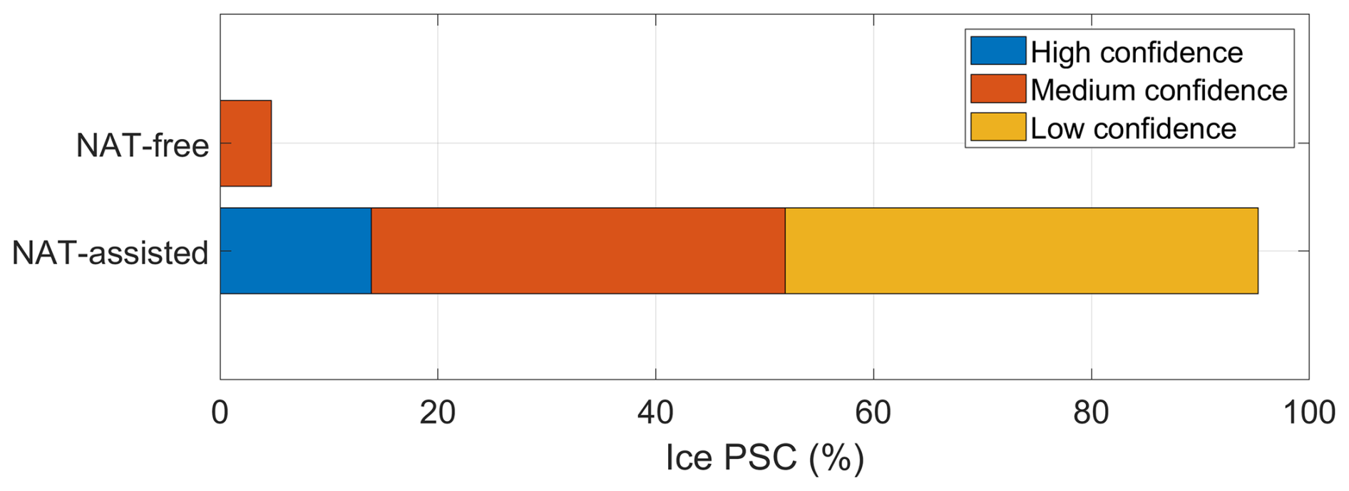
Figure 19 The percentage of ice PSCs formed via NAT-assisted and NAT-free nucleation processes, categorized by confidence levels based on backward-trajectory observations and MLS HNO₃ availability. The bars represent high-, medium-, and low-confidence cases for each process, with confidence levels determined by the presence of NAT and gas-phase HNO₃ concentrations along the trajectories.

Ice PSCs that formed under extremely denitrified conditions are classified as NAT-free ice formation with medium confidence. Here, the backward trajectories reveal very low MLS HNO₃ (<0.5 ppb), creating conditions under which NAT formation is unlikely; thus, ice must have nucleated without the presence of NAT. In this scenario, ice PSCs were likely formed on STS particles with foreign nuclei inclusion. This breakdown helps to clarify the processes of ice formation under varying atmospheric conditions and enhances our understanding of the role that NAT plays in polar stratospheric cloud nucleation. The clear separation into different confidence levels also emphasizes the influence of gas-phase HNO₃ availability on determining the nucleation pathway.

In summary, we report the strong enhancement of aerosol loading in the lower stratosphere caused by the Black Summer event during early 2020. In addition, we observed increased gas-phase MLS HNO₃ and H₂O mixing ratios at an altitude of ∼ 25 and ∼ 17 km, respectively. The increased HNO₃ is due to an enhanced heterogeneous reaction known as N₂O₅ hydrolysis, while increased H₂O is directly injected by smoke plumes from the bushfire. Subsequently, during Austral winter in 2020, an anomalously high PSC areal coverage was observed, suggesting that the modified stratospheric composition of trace gases strongly influenced PSC formation. Despite the relatively high availability of gas-phase HNO₃ during this period compared to previous normal years, the liquid–NAT mixture PSC areal coverage remained within 1 standard deviation with respect to the background mean (2009–2019), whereas the ice PSC areal coverage exceeded 3 standard deviations. To explain this behavior, we calculated the 48 h backward trajectories of ice and liquid–NAT mixture PSCs using the CLaMS trajectory module with hourly ERA5 operational analysis meteorological data. The temperature history, uptake of MLS-observed HNO₃ and H₂O mixing ratios during the formation of these ice/liquid–NAT mixture PSCs, and types of PSCs observed before the observation of these PSCs along the trajectories are studied to understand their formation pathways. Through this analysis, we report with high confidence that 79 % of the liquid–NAT mixture formed via the ice-free nucleation pathway, as an ice PSC was not observed along the trajectory and the temperature of the air parcel never decreased 1.5 K below T_ice (i.e., the minimum temperature required for ice formation) from the time of the “No Cloud (NC)”/STS observation until the time of the liquid–NAT mixture observation along the backward trajectory. This confirms no formation of ice before the observation of the liquid–NAT mixture. Moreover, we report with high confidence that 12 % of the liquid–NAT mixture formed via the ice-assisted nucleation pathway, as an ice PSC was observed by CALIPSO before the formation of liquid–NAT mixture along the trajectory; we further report with low confidence that 9 % of the liquid–NAT mixture formed via the ice-assisted nucleation pathway, as there was no direct CALIPSO observation of an ice PSC before the liquid–NAT mixture but the corresponding temperature decreased 1.5 K below T_ice, indicating the possible involvement of ice during this liquid–NAT mixture formation. The inability of the ERA5 operational analysis to capture the small-scale temperature fluctuations caused by gravity waves and the possible bias in ERA5 temperature may contribute uncertainty to these percentage contributions of formation pathways.

In the case of ice formation, we observed that the depolarization ratio at 532 nm of ice PSCs preceded by STS along the trajectories exhibited a bimodal distribution. The low depolarization ratio mode peaked at 0.07, and the high depolarization ratio mode peaked at 0.26. In contrast, the ice PSC preceded by liquid–NAT mixture along the trajectory exhibited a single mode of the depolarization ratio with a peak occurring at 0.35, which is closer to the high depolarization ratio mode of ice PSC preceded by STS. This hints a the fact that ice with a high depolarization ratio could be the result of the nucleation of ice on NAT particles, whereas ice with a low depolarization ratio could be the result of the nucleation of ice on STS, which is supported by a previous study from Voigt et al. (2018). To check this, we analyzed the availability of gas-phase HNO₃ at the time of the observation of STS, which was observed before ice formation along the backward trajectories, as HNO₃ availability is crucial for NAT formation. The results indicate that ice PSCs with low depolarization ratios formed under denitrified conditions, when the MLS HNO₃ mixing ratio was below 0.5 ppb during the STS observation along the backward trajectories. Under these conditions, NAT particles could not form due to low HNO₃ availability, which is also confirmed by the CLaMS box model run, and this resulted in ice nucleating directly on STS. In contrast, ice PSCs with high depolarization ratios formed under normal conditions, when the MLS HNO₃ mixing ratio exceeded 3 ppb during the STS observation. This sufficient availability of gas-phase HNO₃ led to the formation of NAT particles (again, this is also confirmed by the CLaMS box model run) and to ice nucleating on NAT. Hence, based on the availability of gas-phase MLS HNO₃ and the temperature history, we conclude the ice formation pathways and relative percentage contribution of formation pathways and degree of confidence.

Hence, we report with high confidence that 14 % of the ice is formed through NAT-assisted ice formation, as direct CALIPSO observations of liquid–NAT mixtures are present along the trajectory; we report with medium confidence that 38 % of the ice is formed through NAT-assisted ice formation, as there is significant gas-phase MLS HNO₃ (>3 ppb), suggesting possible NAT formation before the ice formation; and we report with low confidence that 43 % of the ice is formed through NAT-assisted ice formation when HNO₃ levels are between 0.5 and 3 ppb, indicating a lower likelihood of NAT formation. Furthermore, we report with medium confidence that only 5 % of ice PSCs formed via NAT-free ice formation, as they formed under extremely denitrified conditions (HNO₃<0.5 ppb), suggesting less likelihood of NAT formation and, thus, of ice formed via nucleation on STS. This suggests that the availability of gas-phase HNO₃ is a crucial factor in deciding whether ice forms via a NAT-assisted or NAT-free nucleation process. To the best of our knowledge, this is the first study that has provided the relative contributions of various liquid–NAT mixtures and ice formation pathways. These results provide deeper insights into the microphysical processes through which aerosols from extreme bushfire events (like Black Summer) can influence stratospheric chemistry and PSC formation.

5 Conclusions

Australia's extreme bushfire event in 2019–2020, also referred to as Black Summer, injected 0.4 to 2 Tg of aerosols into the stratosphere, initiating a series of events. We carried out an extensive investigation of the impacts of bushfire emissions on polar stratospheric clouds (PSCs), using multi-satellite and reanalyses data. In addition, to explain the observed anomaly in the areal coverage of ice and liquid–NAT mixture PSCs, we investigated their formation pathways by analyzing the temperature history and gas-phase HNO₃ availability. This analysis was performed using Lagrangian backward trajectories of PSC-containing air parcels, coupled with CLaMS microphysical box model simulations, which allowed us to estimate the relative contributions of different formation pathways for these PSC types. The key findings from this study are as follows:

1. During the austral autumn of 2020, we found a significant increase in gas-phase nitric acid (HNO₃) and water vapor (H₂O) (principal constituents of PSCs) from MLS measurements in the high-latitude region of the Southern Hemisphere at altitudes of ∼ 25 and ∼ 17 km, respectively. The former is due to an enhanced dinitrogen pentoxide hydrolysis process, caused by the increased bushfire aerosols, whereas the latter is attributed to the direct injection of water vapor by the Black Summer event.

2. The increase in HNO₃ was expected to enhance HNO₃-containing PSCs, like STS and NAT PSCs. While the areal coverage of STS PSCs peaked significantly, no notable enhancement in liquid–NAT mixture PSCs was observed. However, there was an anomalous increase in the areal coverage of ice PSCs.

3. We report with high confidence that 79 % of liquid–NAT mixtures formed through ice-free nucleation, as no ice PSCs were observed along the backward trajectories and temperature remained above the ice formation threshold (T_ice−1.5 K). Moreover, we report with high confidence that 12 % of liquid–NAT mixtures formed via ice-assisted nucleation, as CALIPSO observations showed ice PSCs before liquid–NAT formation, and we report with low confidence that 9 % of liquid–NAT mixtures formed via ice-assisted nucleation, as the temperature dropped below the ice formation threshold but there was no direct observation of an ice PSC.

4. We observed a bimodal distribution of the depolarization ratio at 532 nm for ice PSCs that are preceded by STS along the backward trajectories. Further analysis of this revealed that a low depolarization ratio mode (peak at ∼ 0.07) corresponds to ice nucleation on STS under denitrified conditions (HNO₃<0.5 ppb). In contrast, a high depolarization ratio (peaked ∼ 0.26) corresponds to ice nucleation on NAT under normal conditions (HNO₃>3 ppb).

5. We report with high confidence that 14 % of ice PSCs formed via NAT-assisted nucleation, as the presence of liquid–NAT mixtures was observed by CALIPSO along the backward trajectory of these ice PSCs; we report with medium confidence that 38 % of ice PSCs formed via NAT-assisted nucleation, as there was no direct CALIPSO observation of the presence of liquid–NAT mixture but there is significant HNO₃ availability >3 ppb, resulting in a high likelihood of NAT formation; and we report with low confidence that 43 % of ice PSCs formed via NAT-assisted nucleation, as HNO₃ levels of between 0.5 and 3 ppb result in a relatively low likelihood of the NAT. Thus, the NAT-assisted ice formation pathway accounts for ∼ 95 % of ice PSCs. In contrast, just 5 % of ice PSCs formed via NAT-free nucleation under extremely denitrified conditions (HNO₃<0.5 ppb), as there was insufficient HNO₃ availability for NAT formation; thus, these ice PSCs should have nucleated on STS with the possible inclusion of foreign nuclei. These results suggest that the ice formation pathway is also decided by the gas-phase HNO₃ availability.

In the context of climate change scenarios, a warming troposphere and cooling stratosphere are expected. The former is expected to increase the frequency of extreme wildfire events, and the latter is projected to enhance the PSC areal coverage, together possibly delaying the ozone recovery process. The findings from this study will contribute to a deeper understanding of the influence of extreme wildfire events on PSC dynamics.