Multi-observational estimation of regional and sectoral emission contributions to the persistent high growth rate of atmospheric CH₄ for 2020–2022

Atmospheric methane (CH₄) growth rates reached unprecedented values in the years 2020–2022. To identify the main drivers of this increase, an inverse modeling study estimated regional and sectoral emission changes for 2016–2022. Three inverse estimates based on different sets of atmospheric CH₄ observations (surface observations only, surface and aircraft observations, and GOSAT observations) consistently suggest notable emission increases from 2016–2019 to 2020–2022 in the tropics (15° S–10° N) (10–18 Tg CH₄ yr⁻¹) and in northern low latitudes (10–35° N) (ca. 20 Tg CH₄ yr⁻¹), the latter of which likely contributed to the growth rate surge from 2020. The emission increase in the northern low latitudes is attributed to emissions in South Asia and northern Southeast Asia, which abruptly increased from 2019 to 2020, and elevated emissions continued until 2022. Meanwhile, the tropical emission increase is dominated by Tropical South America and Central Africa, but emissions were continuously increasing before 2019. Agreement was found in the sectoral estimates of the three inversions in the tropics and northern low latitudes, suggesting the largest contribution of biogenic emissions. Uncertainty reductions demonstrate that the flux estimates in Asia are well constrained by surface and aircraft observations. Furthermore, a sensitivity test with the probable reduction of OH radicals showed smaller emissions by up to 2–3 Tg CH₄ yr⁻¹ in each Asian region for 2020, still suggesting notable emission contributions. These results highlight the importance of biogenic emissions in Asian regions for the persistent high growth rate observed during 2020–2022.

1 Introduction

Atmospheric methane (CH₄) is the second most important greenhouse gas (GHG) after carbon dioxide (CO₂). Sources of atmospheric CH₄ exist at the Earth's surface, consisting of anthropogenic (60 %) and natural (40 %) emissions (Saunois et al., 2020). Meanwhile, the major sink, oxidation with OH radicals, exists in the atmosphere, which makes the lifetime of atmospheric CH₄ relatively short (ca. 9 years; Szopa et al., 2021). The source–sink imbalance determines the global growth rate of atmospheric CH_4. Excess emissions have increased atmospheric CH₄ by more than 250 % relative to the pre-industrial level (WMO, 2023). However, the growth rate of atmospheric CH₄ has not been steady; it decreased from the late 1980s, reaching almost zero during 1999–2006, and then began to increase again starting in 2007 (Rigby et al., 2008). In 2020–2021, the growth rate rose sharply and reached the highest level (>15 ppb yr⁻¹) on record, followed by a continuously large growth rate of 13 ppb yr⁻¹ in 2022, before falling to the pre-surge level of 10 ppb yr⁻¹ in 2023 (Nisbet et al., 2023; Lan et al., 2024). Our understanding of these growth rate changes is insufficient, resulting in many controversial studies (e.g., Peng et al., 2022; Qu et al., 2022). It is imperative to evaluate a probable CH₄ emissions increase or OH sink decrease for 2020–2022. In particular, CH₄ has recently attracted global attention because as a result of its short lifetime, the mitigation effect on global warming when reducing its emissions occurs sooner than when reducing CO₂ emissions. Hence, ambitious reduction targets (reducing emissions by 30 % from 2020 levels by 2030) were envisaged in the Global Methane Pledge for the coming years (Global Methane Pledge, 2025).

Previous studies (Peng et al., 2022; Qu et al., 2022; Stevenson et al., 2022; Feng et al., 2023) found that both increases in CH₄ emissions and decreases in OH radicals contributed to the rise of atmospheric CH₄ in 2020. It is suggested that nitrogen oxide (NO_x) emissions largely decreased due to the lockdowns under the COVID-19 pandemic, and consequently OH radicals decreased globally in that year (e.g., Miyazaki et al., 2021). Peng et al. (2022) and Stevenson et al. (2022) used chemical transport models to estimate that the global drop of OH radicals contributed about half of the atmospheric CH₄ increase in 2020. Meanwhile, although a significant contribution of OH radical was not denied, Qu et al. (2022) and Feng et al. (2023) estimated a larger contribution from an emissions increase. Particularly in 2021, when NO_x emissions had recovered, a CH₄ emissions increase was likely the major driver of the CH₄ increase (Feng et al., 2023). In 2022, NO_x and CO₂ emissions were reduced by the pandemic again, and the degree of decrease was even larger than it was in 2020 in China (Li et al., 2023). However, that OH reduction effect was limited in space (not global) (Liu et al., 2023) and time (only for January–April) (Li et al., 2023), suggesting a continued contribution of CH₄ emissions.

In this study, we investigated probable emission increases that induced the global atmospheric CH₄ surge for the entire period of high growth (i.e., 2020–2022). We took a so-called “top-down” approach, which derives information of emissions changes at the surface from observations of CH₄ mole fractions in the atmosphere. Specifically, we used an inversion method to quantitatively estimate spatiotemporal variations of surface CH₄ emissions with an atmospheric transport model and prescribed OH fields.

Several inversion analyses have been performed to investigate the recent growth in CH₄ emissions. Qu et al. (2022) and Feng et al. (2023) used column-averaged CH₄ data from the Japanese Greenhouse gases Observing SATellite (GOSAT; Kuze et al., 2009; Yokota et al., 2009), which is dedicated to observing CO₂ and CH₄, in their inversions and estimated that emissions from African wetlands had dominantly contributed the recent atmospheric CH₄ increase. The wetland emissions contributions were also suggested by the inversion of Peng et al. (2022), which used in situ and flask air sampling observations at ground-based stations, but the spatial coverage of the increased emissions ranged from the tropics to the Northern Hemisphere. The succeeding inversion of Lin et al. (2024) for 2020–2021 suggested contributions of wetland emissions in tropical Africa and Southeast Asia and attributed them to the La Niña event.

In fact, geospatial differences of increased CH₄ emissions in the previous inversions may have come from insufficient observational coverage and uncertainties. In situ or flask air sampling measurements are precise, but their spatial coverage is limited. In particular, important CH₄ source regions at low latitudes (Asia, Africa and South America) remain poorly covered by observations. Meanwhile, satellite data cover the globe relatively well, but they only provide column-averaged mole fractions in cloud-free conditions. During winter seasons at high latitudes, satellite data are less available due to insufficient sunlight. Furthermore, they often have satellite-specific errors (Schepers et al., 2012). Specifically, different retrieval methods sometimes produce different features in mole fraction data products. Lin et al. (2024) used ground-based observations and data from two different GOSAT products. One is derived from the proxy method of the University of Leicester (Parker and Boesch, 2020), which constitutes the same data that Qu et al. (2022) and Feng et al. (2023) used. The other is from the so-called full-physics retrieval method of the National Institute for Environmental Studies (NIES) (Yoshida et al., 2013). This kind of multi-observation analysis as carried out by Lin et al. (2024) is imperative to infer the observational uncertainties.

Inversions also have measurable uncertainties caused by the atmospheric transport model used as well as the inversion method (Saunois et al., 2020; Stavert et al., 2022). However, a limited number of transport models have been used in the previous studies. For example, Qu et al. (2022) and Feng et al. (2023) used the same transport model (GEOS-Chem), and Peng et al. (2022) and Lin et al. (2024) also used the same transport model (LMDZ-SACS), while Lin et al. (2024) tested different transport model configurations in their inversion analysis.

This study uses an inversion system based on a different transport model from those used in the previous studies. Here we use the Nonhydrostatic Icosahedral Atmospheric Model (NICAM; Satoh et al., 2014)-based Inversion Simulation for Monitoring CH₄ (NISMON-CH₄) (Sect. 2.1). Using NISMON-CH₄, we estimate CH₄ emissions changes from in situ and flask observations as well as from GOSAT data (Sect. 2.3). Moreover, for the in situ and flask data, we use not only data obtained at the surface but also airborne data from various aircraft observations. Using these multiple observational platforms, we carefully evaluate the reliability of the inversions. In addition, posterior flux errors are utilized to quantify observational impacts and the independence of estimated fluxes (Sect. 2.4). Because our focus is on the emissions increase, the inversion analyses were performed with the climatological OH data, under the assumption that the OH field did not change from year to year. However, the effect of the probable OH reduction in 2020 was investigated by performing a sensitivity inversion test (Sect. 2.5).

2 Method

2.1 NISMON-CH₄

The inverse analysis of NISMON-CH₄ uses a four-dimensional variational method (4D-Var) with the offline forward and adjoint modes of NICAM-based Transport Model (NICAM-TM; Niwa et al., 2011, 2017b). A similar inverse simulation for CO₂ using the same system (NISMON-CO₂) is described in detail by Niwa et al. (2017a, 2022). Because the CH₄ inverse analysis of this study adopts almost the same schemes used in Niwa et al. (2022), readers are encouraged to consult it for details. Unlike the traditionally employed rectangular grid system, NICAM has an icosahedral grid system, with hexagon- or pentagon-shaped grids. In this study, the model horizontal resolution is set at “glevel-5”, which has a mean grid interval of approximately 223 km. The number of vertical layers is 40 with the top at approximately 45 km above sea level. The lowest 12 layers cover the altitude range below about 3 km, with which vertical mixing is reasonably simulated (e.g., see Niwa et al., 2011 for ²²²Rn). Meanwhile, the vertical grid spacing in the upper troposphere–lower stratosphere (UT/LS) is relatively coarse (about 1 km), which may cause faster mixing in the UT/LS region. This could affect absolute values of CH₄ emission estimates; however, its influence on the results in this study would be limited because temporal variations of CH₄ emissions are mainly discussed. Atmospheric transport fields to drive the offline NICAM-TM are given by a preliminary run of NICAM, with horizontal winds nudged to match Japanese 55-year Reanalysis data (JRA55: Kobayashi et al., 2015). The chemical reactions of CH₄ are calculated in NICAM-TM with the prescribed chemical data that were used in the TransCom-CH₄ experiment (Patra et al., 2011): the tropospheric OH is reduced by 8 % with respect to the three-dimensional climatological fields of Spivakovsky et al. (2000), and the stratospheric reactions with Cl and O(¹D) are given by parameterized loss rates (Velders, 1995).

In NISMON-CH₄, although atmospheric transport is simulated on the icosahedral grids, fluxes are optimized on 1°×1° latitude–longitude grids through a grid conversion scheme (Niwa et al., 2022). For that flux optimization, a quasi-Newton method with the Broyden–Fletcher–Goldfarb–Shanno (BFGS) algorithm (Fujii, 2005; Niwa et al., 2017a) is used. Unlike the CO₂ inversion of Niwa et al. (2022), an external constraint is newly introduced in the cost function to avoid unrealistic negative values of CH₄ fluxes (or positive fluxes for soil uptakes). The details of this are described in Appendix A.

The inverse calculation period begins on 1 January 2015 with a three-dimensional CH₄ mole fraction field that is optimized by a previous inversion with surface observations (Saunois et al., 2020) and ends on 31 March 2023. To reduce errors induced by the initial mole fraction field (though, it is already optimized to a certain extent), the first 12 months (i.e., the year 2015) is disregarded in post-inversion analyses (i.e., it is the spin-up). Furthermore, the last 3 months (i.e., January–March 2023) is also disregarded because this period might not be fully constrained by observations (spin-down). The 4D-Var method requires iterative calculations to optimize parameters. In the inversions described below, we confirmed that fluxes were well converged at the 200th iteration. Therefore, we commonly analyze flux data from the 200th iteration.

2.2 Flux model and prior flux data

In NISMON-CH₄, the total net CH₄ flux, $f_{{\mathrm{CH}}_{\mathrm{4}}}\left(x,t\right)$, consists of 10 sectoral fluxes (Table 1):

$$\begin{array}{}\text{(1)}& \begin{array}{rl}{f}_{{\mathrm{CH}}_{\mathrm{4}}}\left(x,t\right)& ={\sum }_{i=\mathrm{1}}^{\mathrm{5}}\left[\left(\mathrm{1}+\mathrm{\Delta }{\mathit{\alpha }}_{\mathrm{anth},i}\left(x,t\right)\right)f_{\mathrm{anth},i}\left(x,t\right)\right]\\ & +\left(\mathrm{1}+\mathrm{\Delta }{\mathit{\alpha }}_{\mathrm{bb}}\left(x,t\right)\right)f_{\mathrm{bb}}\left(x,t\right)+\left(\mathrm{1}+\mathrm{\Delta }{\mathit{\alpha }}_{\mathrm{nat}}\left(x\right)\right)\\ & f_{\mathrm{nat}}\left(x\right)+\left(f_{\mathrm{rice}}\left(x,t\right)+\mathrm{\Delta }{f}_{\mathrm{rice}}\left(x,t\right)\right)\\ & +(f_{\mathrm{wetl}}\left(x,t\right)+\mathrm{\Delta }{f}_{\mathrm{wetl}}\left(x,t\right))-(f_{\mathrm{soil}}\left(x,t\right)\\ & +\mathrm{\Delta }{f}_{\mathrm{soil}}\left(x,t\right)),\end{array}\end{array}$$

where x and t represent flux location and time, respectively. Optimizing parameters are described by Δα and Δf, which represent a modification factor and a flux deviation to each a priori sectoral flux, respectively. The first term on the right-hand side denotes the sum of five anthropogenic (anth) emissions ($i=\mathrm{1},\mathrm{2},\mathrm{\dots },\mathrm{5}$): coal mining (coa), oil–gas exploitation and use (ogs), landfill and waste (lfw), biofuels (bfl), and enteric fermentation and manure management (agr). Their prior fluxes f_anth,i are taken from the annual mean data of Emissions Database for Global Atmospheric Research (EDGAR) version 6.0 (Crippa et al., 2021; Monforti-Ferrario et al., 2021). The temporal resolution of each Δα_anth,i is annual. This is because, although f_anth,i has some seasonal variability, its magnitude is 1 or 2 orders smaller than those of fire, wetland, or rice emissions. The second term is biomass burning (bb) emissions, and its prior flux f_bb is from the Global Fire Emission Database (GFED) v4.1s (van der Werf et al., 2017). The temporal resolutions of Δα_bb as well as f_bb are monthly. The third term represents natural (nat) emissions (the sums ocean, termite, and geological emissions); their prior fluxes f_nat are derived from Weber et al. (2019), Ito (2023), and Etiope et al. (2019), respectively (the geological emissions are scaled so that the global total is 23 Tg according to Canadell et al., 2021). Because their interannual variations are highly uncertain and their contributions are minor compared to the other fluxes, f_nat and Δα_nat are set to be temporally constant throughout the analysis period. The latter three terms are monthly emissions of rice cultivation, wetland, and soil uptakes, and their prior fluxes, f_rice, f_wetl, and f_soil, are given by the terrestrial biosphere model Vegetation Integrative SImulator for Trace gases (VISIT; Ito and Inatomi, 2012). The fluxes used in this study are calculated with the scheme of Cao et al. (1996) for f_rice and f_wetl. As of the start of this study, the data from EDGAR (f_anth,i) and VISIT (f_rice, f_wetl and f_soil) were available through 2018 and 2020, respectively. For the later years, we used data from the final year they were available. Consequently, during the period of 2020–2022, which is the focus of this study, prior fluxes other than the biomass burnings do not have interannual variations. Therefore, in the inversions, interannual variations of estimated emissions are mostly derived from observations.

As shown in Eq. (1), the flux optimization parameters are constructed by mixing scaling factors (Δα) and the flux deviations (Δf). In fact, they are applied to spatially small-scale (f_anth,i and f_bb) or minor (f_nat) fluxes and to those with relatively broad-scale variations (f_rice, f_wetl, and f_soil), respectively. The scaling factor only modifies flux magnitudes but not distributions because the inversion may not be able to modify small-scale distributions reliably due to the nature of atmospheric mixing.

In the inversion, the prior errors of the scaling factors are set at 50 % for Δα_anth,i and 100 % for Δα_bb and Δα_nat assuming no spatiotemporal error correlation. The prior errors and error covariances of Δf_rice, Δf_wetl, and Δf_soil are derived from ensembles. Each ensemble is calculated from a 120-year-long simulation (1901–2020) of VISIT, in which data in each year are considered as one member. A similar method is used in NISMON-CO₂ and is detailed in Niwa et al. (2022). In this method, not only variance but also covariances are calculated from the ensemble. However, they are localized in space by a Gaussian function to damp erroneous correlations in remote areas. Here, we also assumed no temporal correlation. Those prior errors and covariances are combined to construct a prior error covariance matrix, B, with which the cost function of the inversion is defined. The annual global totals and their integrated errors of the prior fluxes are presented in Table 1.

Table 1 Categorization of CH₄ fluxes and their global totals for 2020.

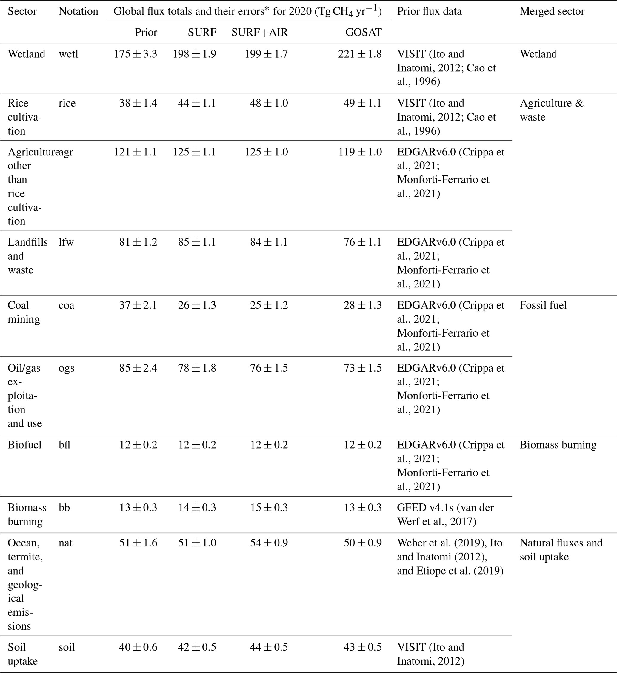
^* The annual global error was calculated as $\sqrt{{\mathit{g}}^T\mathbf{B}\mathit{g}}$, where B is a prior (posterior) error covariance matrix, and g is the spatiotemporal integration operator vector. Because this is derived from a summation of variances (squared values), it should be noted that the rank order of their magnitudes should be different from that of the global flux totals.

2.3 Observations

2.3.1 Surface and aircraft data

In this study, we performed two inversions with in situ and flask observations (listed in Supplement Materials S1 and S2): one uses only surface observations (SURF), and the other uses both surface and aircraft observations (SURF+AIR). These in situ and flask data were obtained from version 6.0 of ObsPack GLOBALVIEWplus (Schuldt et al., 2023a). In addition, data from version 6.0 of ObsPack Near Real Time (NRT) (Schuldt et al., 2023b) were also used for 2023 (spin-down period). For these ObsPack datasets, we only used data with the large-scale representing flag. Furthermore, we used additional data from NIES and collaborative networks: flask air sampling observations at Asian stations (Tohjima et al., 2002, 2014; Nomura et al., 2017, 2021; Okamoto et al., 2018); flask and in situ continuous observations on voluntary observing ships (VOSs) in the Pacific, in Oceania, and around Southeast Asia (Terao et al., 2011; Nara et al., 2017); and flask observations by aircraft over Siberia (Sasakawa et al., 2017). We also used in situ continuous data from the Japan–Russia Siberian Tall Tower Inland Observation Network (JR-STATION) operated by NIES (Sasakawa et al., 2010) (only daytime (13:00–17:00 LT) data were used) and flask observations from the aircraft programs of the Comprehensive Observation Network for TRace gases by AIrLiner (CONTRAIL; Machida et al., 2008; Matsueda et al., 2015; Sawa et al., 2015; Umezawa et al., 2012) and Tohoku University (Umezawa et al., 2014).

The ObsPack datasets provide CH₄ mole fractions on the WMO CH₄ X2004A scale (Dlugokencky et al., 2005), while the NIES and CONTRAIL data are provided on the NIES94 CH₄ standard scale, which is approximately 5 ppb higher than the WMO scale (Machida et al., 2023). The aircraft data from Tohoku University are based on the TU-1987 scale, which is deemed to be comparable to the WMO scale (the difference is about 0.5 ppb, Fujita et al., 2018). In this study, we commonly use the CH₄ observations on the WMO scale; we modified the NIES-94 scale data to the WMO scale using the linear relationship reported in Tsuboi et al. (2017).

Figure 1a shows the geographic locations of surface observations used in SURF. Here, we use almost all available data from the ObsPack datasets for 2015–2023, but we use only the highest-altitude data for tower sites that provide data for multiple altitudes. The ship observations that cover the northern Pacific, Asia, and Oceania regions are from the NIES VOS program. Note that data at each site in Fig. 1a are not always available for the whole period, which could affect flux estimates in inversion.

The locations of the aircraft data used in SURF+AIR are depicted in Fig. 1b. The network covers various regions by many campaign flights, such as by ACT America (Wei et al., 2021; Davis et al., 2018). The National Oceanic and Atmospheric Administration (NOAA) and Japan Meteorological Agency (JMA) operate regular aircraft observations at fixed areas over North America (Sweeney et al., 2015) and the western North Pacific (Tsuboi et al., 2013; Niwa et al., 2014), respectively. Observations using commercial airliner are also regularly operated by CONTRAIL and In-service Aircraft for a Global Observing System (IAGOS: Schuck et al., 2012; Petzold et al., 2015), but their flight routes change frequently. Nevertheless, CONTRAIL has continuously provided data from around Asian regions during the analysis period. Aircraft often enters the lower stratosphere (LS), and this is especially true for commercial flights because they fly at higher altitudes (∼ 10 km). Variations of CH₄ in LS are largely affected by the stratospheric circulation, and consequently, their seasonal patterns differ largely from those in the upper troposphere (UT) (Sawa et al., 2015). Therefore, we use only tropospheric data for the aircraft observations. For the data selection, we use a potential vorticity (PV) criterion of 2 PVU (1 PVU $={\mathrm{10}}^{-\mathrm{6}}$ m² s⁻¹ K kg⁻¹), which is from the NICAM simulation; observations where absolute values of simulated PV were larger than 2PVU were excluded.

As shown in Fig. 1a, the observation network is dense in Europe and North America, while regions such as South America and Africa have fewer observations. Furthermore, in situ and flask data have different temporal resolutions; typically, they are hourly and (bi-)weekly, respectively, at ground-based stations. Such data inhomogeneity due to different measurement methodologies also exists in the aircraft observations. In the inversions, we therefore introduce observational weighting, in which a diagonal element of the observation–model mismatch error covariance matrix (here assumed as a diagonal matrix), R, is defined as

$$\begin{array}{}\text{(2)}& R_{ii}=(\mathit{\beta }{r}_i{)}^{\mathrm{2}}{N}_i,\end{array}$$

where N_i denotes the number of observations within a certain spatiotemporal range of the ith observation. In this study, the range is set at 1 week, a 1000 km horizontal diameter circle, and a 1 km vertical depth. The diagonal matrix of R assumes that all observations are independent from each other. However, that is not necessarily the case, especially where observations are obtained with high density. Therefore, we inflate the variance for such areas with N_i. In fact, Niwa et al. (2022) confirmed that this variance inflation improved inversion results. r_i represents the standard deviation of mole fraction variations of the ith observation (from 1 week before to 1 week after at the same location), which is derived from the NICAM simulation with prior fluxes or observations (the larger one is chosen). β is a tuning parameter to balance the weight with the prior estimate and is here set at 0.5 so that ${\mathit{\chi }}^{\mathrm{2}}(=\frac{\mathrm{2}{J}_{\min }}{m})$, where J_min is the minimum of the cost function, and m is the number of observations, should be less than 1. Both the SURF and SURF+AIR inversions use Eq. (2) with the same configuration. Through Eq. (2), although in situ and flask observations are high-precision, and their uncertainties are within a few parts per billion (ppb), an observation–model mismatch error (the square root of R_ii) reaches over 100 ppb where observations are densely existing.

2.3.2 GOSAT

We also used GOSAT column-averaged dry-air mole fraction (XCH₄) data from the full-physics retrieval of NIES (Yoshida et al., 2011, 2013); they are provided as a GOSAT Level 2 (L2) CH₄ product from short-wavelength infrared (SWIR) spectral data observed by GOSAT Thermal And Near infrared Sensor for carbon Observation-Fourier Transform Spectrometer (TANSO-FTS). The version 2.95/96 for General Users was used. Compared to the proxy method (Parker and Boesch, 2020), the full-physics method uses a radiative transfer model that considers multiple scattering by aerosols and clouds explicitly. Although the number of observations that are well retrieved is smaller, the full-physics method is less sensitive to prior model CO₂ data than the proxy method (Schepers et al., 2012). As shown in Fig. 1c, GOSAT data cover the globe well between 60° S and 60° N, but the latitudinal range of data available changes seasonally because of sunlight (data higher than approximately 45° N are not available during northern winter). In the inversion, we used all available data including sunglint condition data; they were all corrected in advance by the bias evaluation of Inoue et al. (2016) (NIES GOSAT Project, 2023). Although the data availability differs by seasons, the GOSAT observations have been more constantly obtained from one year to another than the in situ or flask observations.

The GOSAT inversion of NISMON-CH₄ has the satellite-specific observational operator between the simulated and observed mole fractions. A simulated dry-air column-averaged mole fraction corresponding to a GOSAT observation, X^sim, is calculated from a vertical profile of simulated dry-air mole fractions, c^sim, as

$$\begin{array}{}\text{(3)}& X^{\mathrm{sim}}={\mathit{w}}^T\mathbf{A}\left(\mathbf{G}{\mathit{c}}^{\mathrm{sim}}-{\mathit{c}}^{\mathrm{pri}}\right)+{\mathit{w}}^T{\mathit{c}}^{\mathrm{pri}},\end{array}$$

where w is a weighting vector based on pressures. The matrices of A and G are an averaging kernel matrix and a remapping matrix from the model vertical layers to the GOSAT retrieval layers, respectively, and c^pri is a vertical profile vector of CH₄ dry-air mole fractions that is used as a priori in the retrieval. A and c^pri are provided with the GOSAT-L2-SWIR product.

Because GOSAT has relatively homogeneous data in space and time compared to the in situ and flask observations, we do not employ the observational weighting of Eq. (2) in the GOSAT inversion. Instead, we commonly set the observation–model mismatch error (the square root of a diagonal element of the error covariance) as 20 ppb for every observation. In fact, it is larger than the probable error of the GOSAT data (NIES GOSAT Project, 2023). This error inflation is intended to implicitly consider error correlations among nearby observations. As is done for the SURF and SURF+AIR inversions, off-diagonal elements of the error covariance matrix are set at zero.

Although the GOSAT data are corrected separately for land and ocean (NIES GOSAT Project, 2023), it is known that some spatial (e.g., latitudinal) biases still exist in the satellite data, which are often corrected before inversion by referring to an independent inversion with high-precision in situ/flask observations (Bergamaschi et al., 2007; Meirink et al., 2008). In this study, we did not apply this type of bias correction for the GOSAT data; therefore the SURF/SURF+AIR and the GOSAT inversions remained independent. The probable spatial bias of the GOSAT data is discussed in Appendix B.

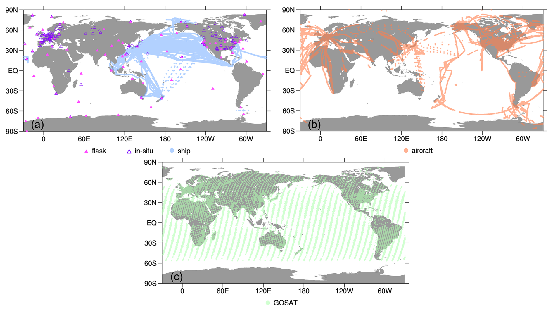
Figure 1 Locations of the observations used in the inverse analyses. In situ (open triangles) and flask air (closed triangles) measurements at surface stations and ship (light-blue dots) data for January 2015–March 2023 are shown in (a), and those for aircraft (orange) are shown in (b). The GOSAT data (light green) shown in (c) are obtained during 2020, which has a similar pattern to the other years.

2.4 Posterior errors

Observational constraints in the inversions are quantified by using posterior errors. Posterior errors are derived from diagonal elements of the posterior error covariance matrix, P, which can be written with the error covariance matrices B and R and with the linear model operator matrix of atmospheric transport M (including the observational operator and the flux model) as

$$\begin{array}{}\text{(4)}& \mathbf{P}={\left({\mathbf{B}}^{-\mathrm{1}}+{\mathbf{M}}^T{\mathbf{R}}^{-\mathrm{1}}\mathbf{M}\right)}^{-\mathrm{1}}.\end{array}$$

Because the matrix size of Eq. (4) is extremely large in the 4D-Var method, which optimizes flux parameters at each grid (1°×1° in this study), it is impossible to analytically calculate Eq. (4). Therefore, we use the approximation method of Niwa and Fujii (2020) to estimate each element of P, which uses the BFGS formula with vector pairs generated from ensemble calculations and orthogonalization. This method can estimate P accurately, not only for diagonal but also for off-diagonal elements for a linear problem. In fact, the inverse problem in this study is nonlinear because an additional constraint is introduced to avoid negative values (Appendix A). Therefore, to estimate P, we omit the nonlinear additional constraint. Furthermore, we calculate P only for the year 2020 due to the high computational demand. In the three inversion cases, we performed 50 iterations with 120 ensemble members. From the 6000 vector pairs generated, we obtained approximately 900 conjugate vector pairs by orthogonalization. Those conjugate vector pairs were used to estimate P with the BFGS formula. Then, we applied spatiotemporal aggregation, as was done for the posterior fluxes:

$$\begin{array}{}\text{(5)}& {\mathbf{P}}^{\mathrm{agr}}={\mathbf{DPD}}^T,\end{array}$$

where D and P^agr are an aggregation operator matrix and an aggregated posterior error covariance matrix, respectively. The square root of the ith diagonal element of P^agr is the posterior error of the ith aggregated flux parameter, ${\mathit{\sigma }}_i^{\mathrm{pos}}$. Its error reduction ratio from a corresponding prior error ${\mathit{\sigma }}_i^{\mathrm{pri}}$ defined as

$$\begin{array}{}\text{(6)}& e_i={\displaystyle \frac{\left({\mathit{\sigma }}_i^{\mathrm{pri}}-{\mathit{\sigma }}_i^{\mathrm{pos}}\right)}{{\mathit{\sigma }}_i^{\mathrm{pri}}}}\times \mathrm{100}\end{array}$$

can be used to quantify the strength of the observational constraint imposed on the ith flux parameter; a larger e_i means a stronger constraint by observations. Furthermore, an off-diagonal element of P^agr derives an error correlation between two flux parameters, which could indicate how independently a flux parameter is optimized in inversion.

2.5 Sensitivity tests

To investigate the effects of the probable OH reduction due to the pandemic in 2020, we performed an extra inversion analysis with a modified OH field. The methods and results of this analysis are described in Appendix C. Furthermore, we also performed inversion analyses with different datasets of in situ and flask observations as well as GOSAT retrieval. The details of the observations and the results of these inversions are described in Appendix D.

3 Results

3.1 Evaluation of posterior mole fractions

Before evaluating the posterior fluxes, we evaluated the consistency of posterior atmospheric CH₄ mole fractions globally with observations to assess the validity of our inversions. For the evaluation, we calculated correlations and root-mean-square differences (RMSDs) between the model and the observations for the northern high and low latitudes (35–90° N, 10–35° N), the tropics (15° S–10° N), and the southern latitudes (90–15° S).

For the reference observations, we used flask air sampling observations from surface sites (including ships) and aircraft, which are part of the observations used in the inversions. The in situ data were not used to avoid excessive weights of those data on the evaluation. Furthermore, the flask-sampling data at Comilla, Bangladesh, were excluded because the observed mole fractions at Comilla were known to have extremely large variations (Nomura et al., 2021), and the observation–model mismatch would induce a large weight of South Asia in the statistics (note that the Comilla data were used in the inverse analysis because Eq. (2) made observational weights flatter). For the aircraft data, we used only data from over 3 km altitude to represent the free troposphere.

In addition, we also used the same GOSAT data used in the inversion. Before calculating the statistics, we subtracted the averages for 2016–2019 from the modeled and observed mole fractions, respectively, for each latitudinal band, which excludes temporally and spatially varying biases of the GOSAT data that may still exist after the globally uniform bias correction. However, as shown in Appendix B, we found notable systematic differences between the SURF (or SURF+AIR) and GOSAT inversions. Therefore, in this study, we only discuss differences of fluxes or atmospheric CH₄ from their averages for the former period (2016–2019) by latitude or region. This could cancel the spatial biases of GOSAT and enabled us to focus on the increases in fluxes or mole fractions for 2020–2022, which is the target of our study.

Figure 2 shows the calculated correlations and RMSDs between the simulated and observed atmospheric CH₄. In most cases, the posterior correlations and RMSDs are larger and smaller, respectively, than those of priors, indicating that the inversions appropriately incorporated the observations in their flux optimizations. In particular, the larger correlations and smaller RMSDs with independent observations (i.e., those not used in the inversion) suggest that posterior CH₄ fluxes have improved atmospheric CH₄ fields relative to the prior ones. The GOSAT inversion shows little improvement of or even worse correlations and RMSDs when evaluated against the surface observations. However, it has clearly better correlations and RMSDs against the aircraft observations than the prior ones, which are even better than the SURF inversion. This is attributable to the fact that both the aircraft observations and the column-averaged observations of GOSAT better represent well-mixed conditions in the free troposphere than the surface observations; therefore, their footprints might be more similar to each other than to those of the surface observations. Furthermore, this result also suggests that GOSAT observations, which may have some biases (Appendix B), could provide constraints to CH₄ emission variations as well as those of in situ and flask observations.

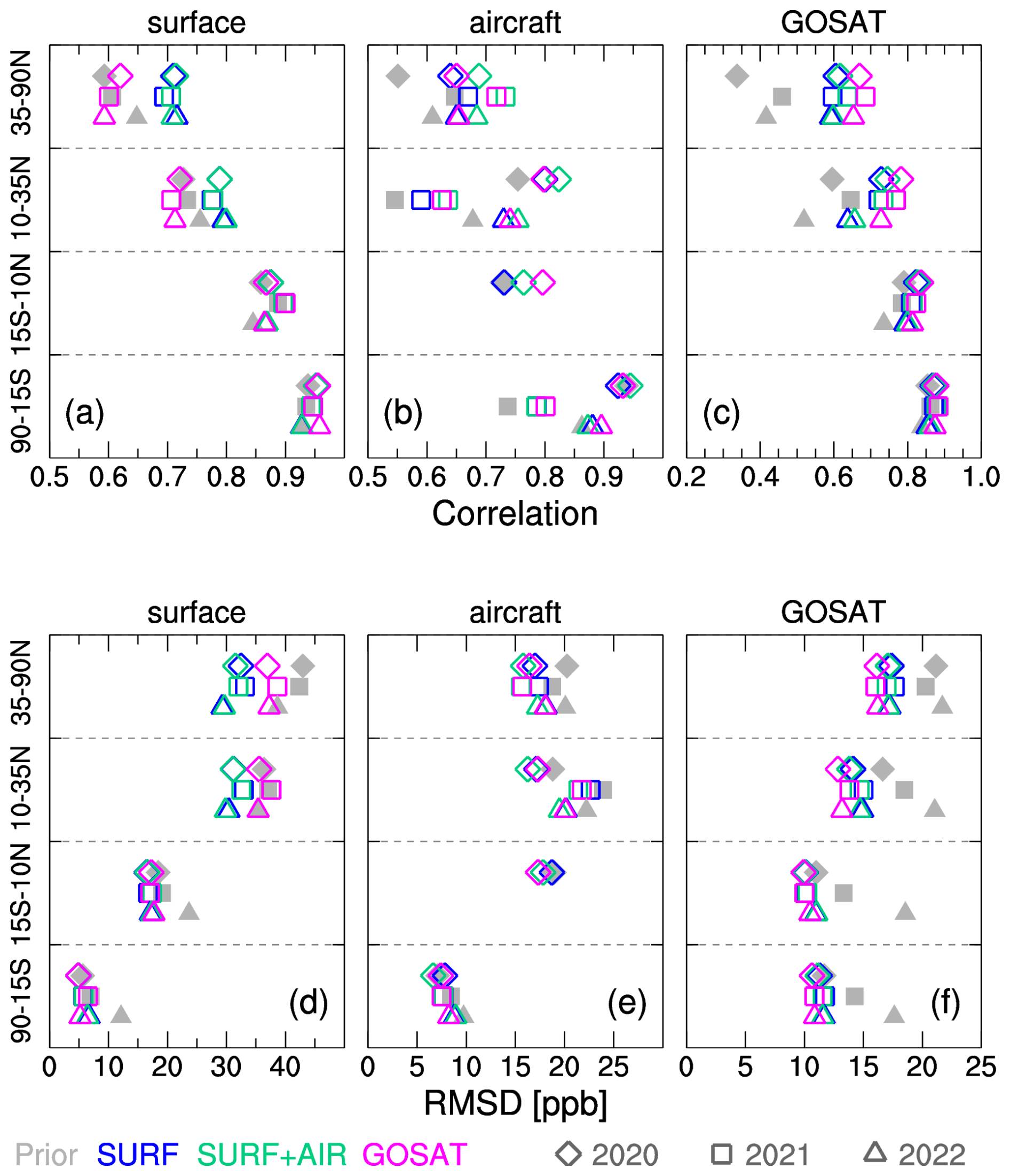
Figure 2 Pearson correlation coefficients (a, b, c) and root-mean-square-differences (RMSDs) (d, e, f) between observations and prior or posterior mole fractions of atmospheric CH₄ in northern high latitudes (35–90° N), northern low latitudes (10–35° N), tropics (15° S–10° N), and southern latitudes (90–15° S) for 2020 (diamonds), 2021 (squares), and 2022 (triangles). The correlations and RMSDs are calculated for surface (directly from all observations in each latitudinal band (with Comilla excluded)) (a, d) and aircraft (>3 km) (b, e) flask observations, as well as for the GOSAT data (c, f). The prior and posterior mole fractions are derived from atmospheric simulations of NICAM-TM with the prior and posterior (SURF, SURF+AIR, and GOSAT) fluxes, respectively. Before the calculations for correlations and RMSDs, the average for 2016–2019 is subtracted from the observations and simulated mole fractions for 2020–2022 for each observational type in each latitudinal band, which would remove the biases shown in Fig. B2 to show only variations from the reference period of 2016–2019.

3.2 Global features

Figure 3 shows the spatial patterns of the posterior total net CH₄ emissions for the 2016–2019 pre-growth period as well as the patterns of the (posterior − prior) differences. In general, the estimated spatial patterns are consistent in the three inversions, but the differences display different features between the SURF or SURF+AIR inversion and the GOSAT inversion (Fig. 3b–d). Specifically, the tropical (e.g., Central Africa and Tropical South America) fluxes are noticeably larger, and the northern mid-latitude fluxes are smaller than the prior fluxes for the GOSAT inversion. Meanwhile, those of SURF and SURF+AIR are rather consistent with the prior fluxes. Therefore, the GOSAT inversion has systematically larger emissions in the tropics than the other two inversions. In the northern high latitudes, the opposite case is true; the SURF and SURF+AIR inversions estimated larger emissions in Siberia than the GOSAT inversion. These latitudinal differences of the estimated emissions are attributable to the systematic differences between the in situ or flask observations and the GOSAT observations shown in Appendix B.

Despite such differences among the posterior fluxes, the three inversions showed the same tendency of sectoral emission changes with respect to the prior data, such as larger wetland and rice cultivation emissions and smaller coal mining and oil–gas emissions (Table 1). The errors of those emissions were reduced with respect to the prior ones, indicating that those emission changes were constrained by observations. However, it should be noted that the posterior errors are generally smaller than the differences among the three inversions. In addition, they are also smaller than an inversion ensemble spread (e.g., Saunois et al., 2025). Therefore, those calculated posterior errors cannot be considered as practical uncertainties of the inversion.

From 2016–2019 to 2020–2022, spatial patterns of the CH₄ emission increases are also consistent in the three inversions (Fig. 4). Hereafter, we refer to a difference of CH₄ emissions from the 2016–2019 mean as ΔfCH₄. In Fig. 4, the area with notable positive ΔfCH₄ values ranges from the tropics to the northern high latitudes. The increase in the northern low latitudes (10–35° N) is particularly noteworthy; the three inversions consistently estimate that northern South Asia (Bangladesh and northern India) and Mainland Southeast Asia were major contributors to the increase. Meanwhile, in the northern high latitudes (35–90° N) and topics (15° S–10° N), areas with a large emissions increase are also consistently estimated, but their magnitudes differ, especially between the SURF or SURF+AIR inversion and the GOSAT inversion. For example, emissions in the northern North America and Sahel regions are estimated as smaller and larger, respectively, in the GOSAT inversion.

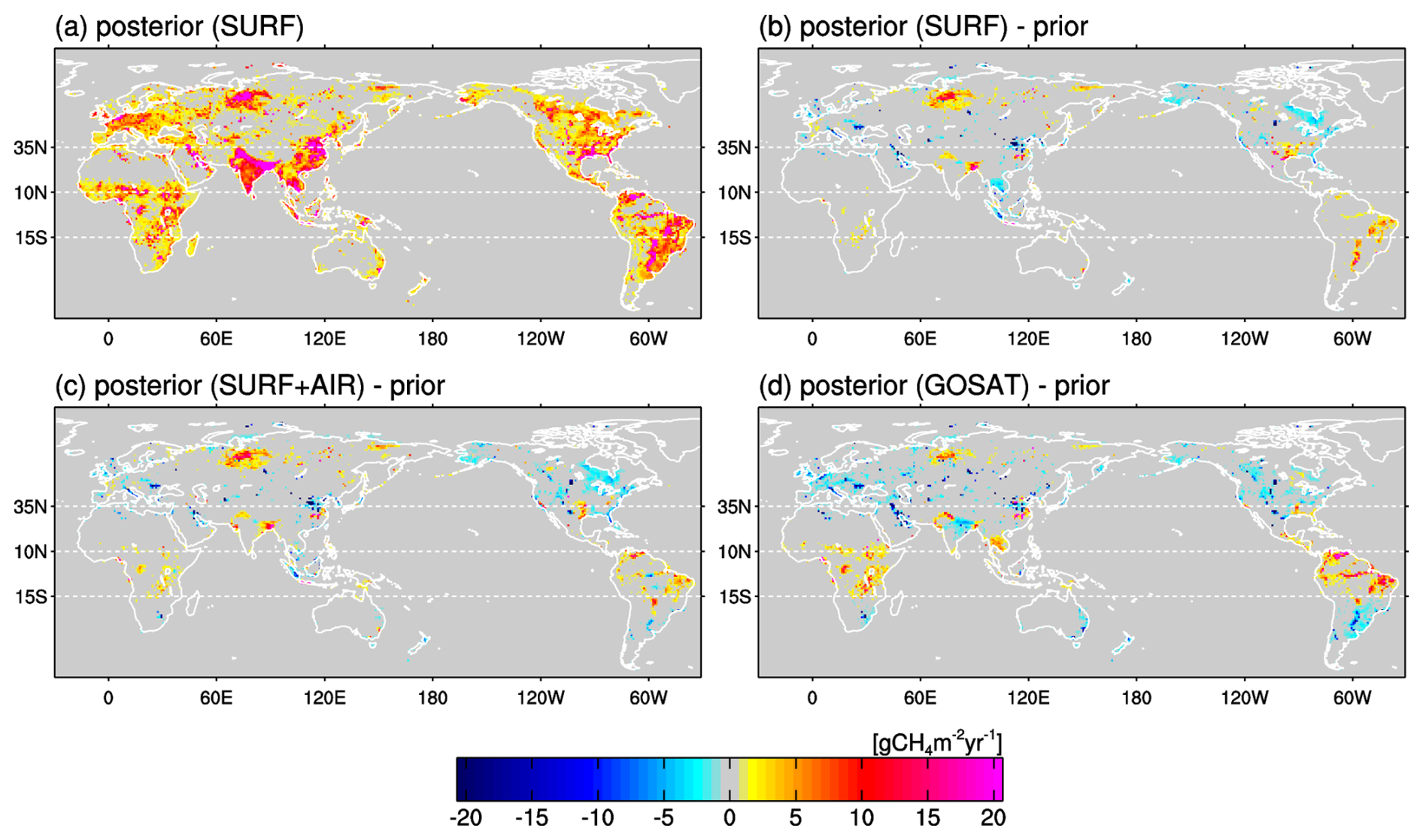
Figure 3 Spatial pattern of posterior total net CH₄ emissions by the SURF inversion averaged for 2016–2019 (a) and the (posterior − prior) difference pattern (b). Also shown are the other (posterior − prior) emissions patterns for the SURF+AIR (c) and GOSAT (d) inversions.

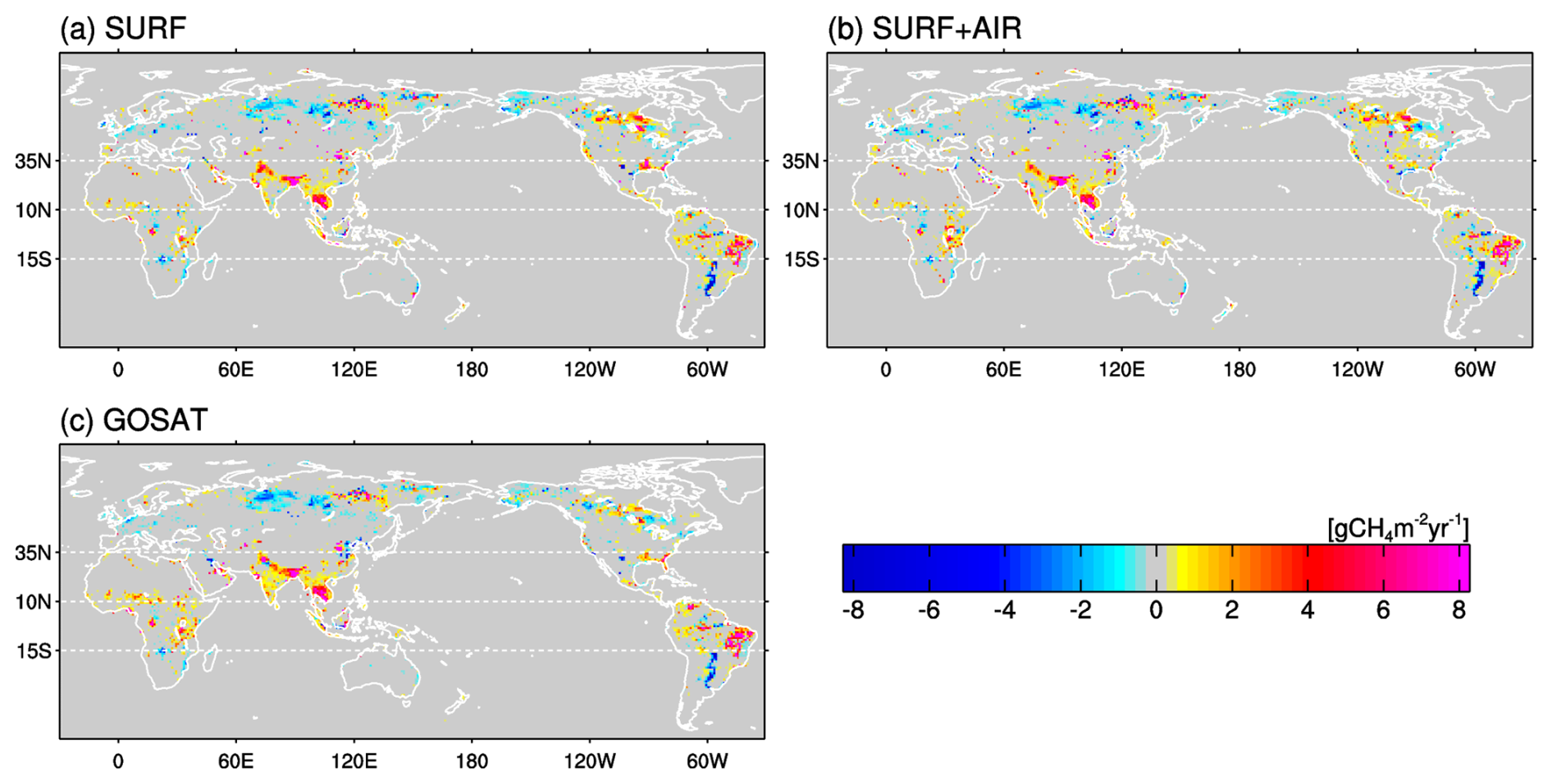
Figure 4 Spatial patterns of the total net CH₄ emissions increase (ΔfCH₄) from 2016–2019 to 2020–2022 in the SURF (a), SURF+AIR (b), and GOSAT (c) inversions.

Year-to-year variations of the global total net CH₄ emissions are also consistently estimated by the inversions for 2016–2022 (Fig. 5a). Their temporal patterns are similar to those of the global growth rate observed in the marine boundary layer sites of NOAA (Lan et al., 2024); in 2020, the global total net emissions abruptly increased by approximately 30 Tg CH₄ yr⁻¹, followed by a similar magnitude or even greater increased emissions in 2021. In 2022, the emissions decreased but remained greater than the pre-2020 level. In 2021, when the inversions showed the highest emissions, the estimates differ, largely ranging from 592 (SURF) to 603 Tg CH₄ yr⁻¹ (GOSAT). Also, in the three different latitudinal bands, ΔfCH₄ changes are consistently estimated (Fig. 5b–e). The increase in the northern low latitudes is noteworthy; it displays a sharp rise from 2019 to 2020, and large emissions continue through 2022, when the magnitudes (ca. 20 Tg CH₄ yr⁻¹) are consistent among the inversions. Also, in the tropics, the inversions consistently show increases of 10–18 Tg CH₄ yr⁻¹ in 2020–2022; however, there are gradual increases from 2016, but they do not largely contribute to the global surge in 2020. Meanwhile, in the northern high latitudes, SURF and SURF+AIR estimated a marginal increase that has a peak of 9 Tg CH₄ yr⁻¹ in 2021, while GOSAT estimated smaller increases of 2 Tg CH₄ yr⁻¹. In the southern latitudes, all the inversions do not show any notable change during 2016–2022.

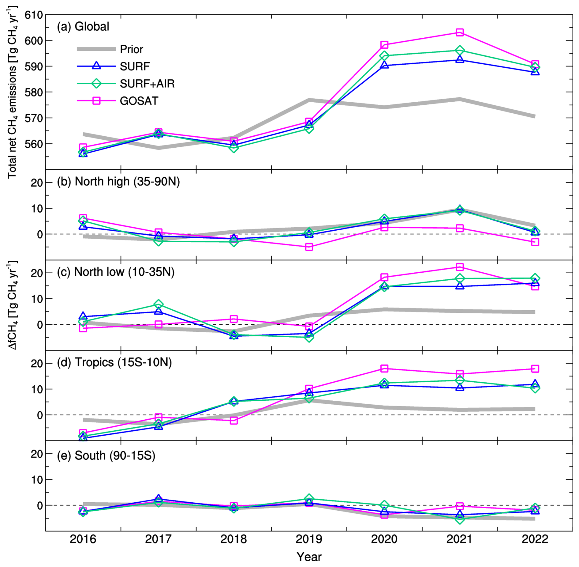
Figure 5 Year-to-year variations of total net CH₄ emissions integrated globally (a) and those of ΔfCH₄ integrated in each latitudinal band: northern high latitudes (35–90° N) (b), northern low latitudes (10–35° N) (c), tropics (15° S–10° N), and southern latitudes (90–15° S) (e).

3.3 Regional features

Figure 6 shows a further regional breakdown of the ΔfCH₄ changes. Figure 6 shows that, in general, even for these smaller regions, the three different inversions consistently show temporal variations of ΔfCH₄. In particular, the consistency between the SURF and SURF+AIR inversions and the GOSAT inversion is noteworthy, because the in situ or flask observation and the GOSAT data were independently obtained. The result indicates that those observations consistently captured atmospheric CH₄ variations that were likely caused by emission changes.

Specifically, in northern Southeast Asia and South Asia, both of which are located in the northern low latitudes (10–35° N), the abrupt increase in ΔfCH₄ by 5 Tg CH₄ yr⁻¹ or more in 2020 and its continuation until 2022 are consistently estimated by all the inversions. This suggests that these two regions are dominant contributors to the recent surge of atmospheric CH₄. Meanwhile, in West Asia, the drop in 2019 is notable and is also estimated consistently by the inversions. In Northern Africa, the SURF+AIR and GOSAT inversions estimated marginal increases in CH₄ (ca. 3 Tg CH₄) in 2020, while SURF estimated a more moderate and gradual increase until 2022. Meanwhile, the inversions show ΔfCH₄ increases of up to 4 Tg CH₄ yr⁻¹ in East Asia for 2020–2021, although the GOSAT inversion shows larger interannual variations during the analysis period. These flux changes may also have contributed to some extent to the surge of atmospheric CH₄ in 2020.

Two regions, Central Africa and Tropical South America, contribute to the gradual increases in ΔfCH₄ in the tropics (Fig. 5d). Meanwhile, ΔfCH₄ also increased in southern Southeast Asia but only during the middle of the analysis period (2019–2021). Although there are some discrepancies, these features of tropical emissions are commonly seen in the three inversions. The relatively large increase in ΔfCH₄ in Central Africa, which is only estimated by the GOSAT inversion, might have contributed to the surge of atmospheric CH₄ but only for 2020.

In the northern high-latitude areas, moderate increases of up to 3 Tg CH₄ yr⁻¹ are estimated in the west part of Northern Eurasia for 2020 and in Boreal North America for 2020–2021 by SURF and SURF+AIR, but these increases are not clearly seen in GOSAT. The east part of Northern Eurasia shows a notable peak in 2021, with magnitudes of 5 and 2 Tg CH₄ yr⁻¹ in SURF or SURF+AIR and GOSAT, respectively.

For other areas such as Europe, the western part of Northern Eurasia, Temperate North America, Central America, Southern Africa, Oceania, and Temperate South America, the inversions suggested that CH₄ emissions did not clearly contribute to the increase in atmospheric CH₄ during 2020–2022.

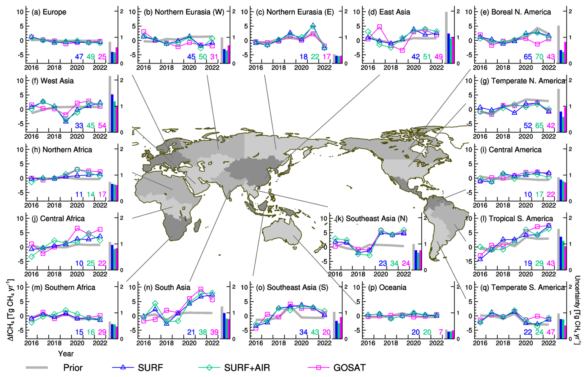
Figure 6 Year-to-year variations of regional ΔfCH₄ (left) and regional annual flux uncertainty for 2020 (right). Emissions are integrated within each geographical region defined in the centered map, which is the same as that used in Canadell et al. (2021), except that Northern Eurasia and Southeast Asia are further divided by west–east and north–south. The numbers in each panel denote the uncertainty reduction ratio (%) of the annual flux for 2020 in each region, with the color corresponding to that of ΔfCH₄.

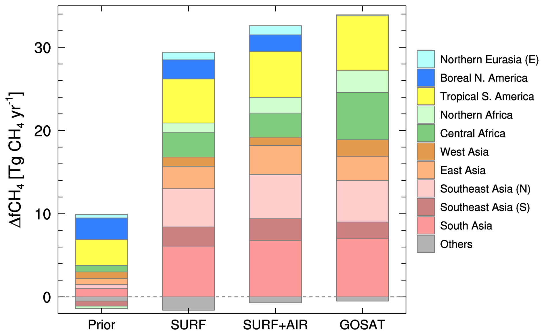
Figure 7 Cumulative bar chart of ΔfCH₄ for 2020–2022 estimated by the prior data and the three inversions (SURF, SURF+AIR, and GOSAT). Contributions from regions where notable emissions changes occurred (Fig. 6) are noted by the colored areas and the others are aggregated into the gray “Others” category. If a mean ΔfCH₄ is positive (negative), it is accumulated upward over (downward under) the dashed zero line.

The regional ΔfCH₄ for 2020–2022 estimated by the inversions is summarized in Fig. 7. In total, the SURF and GOSAT inversions estimated emission increases of 29 and 34 Tg CH₄ yr⁻¹, respectively. The SURF+AIR inversion estimated an intermediate value of 32 Tg CH₄ yr⁻¹. Three regions – South Asia, northern Southeast Asia, and Tropical South America – are commonly presented as major contributors; their estimated emission increases are 6–7, 5, and 5–7 Tg CH₄ yr⁻¹, respectively. The SURF and SURF+AIR inversions suggested the northern regions (Northern Eurasia (E) and Boreal North America) as marginal contributors, but their contributions estimated by the GOSAT inversion are much smaller. Meanwhile, estimated contributions from the African regions (Northern Africa and Central Africa) are larger for GOSAT (3 and 6 Tg CH₄ yr⁻¹, respectively) than for the other two inversions (1–2 and 3 Tg CH₄ yr⁻¹, respectively). Interestingly, all the inversions agree with each other in that the five Asian regions contributed by approximately 60 % of the global ΔfCH₄ increase.

In fact, these estimated regional ΔfCH₄ increases may have non-negligible uncertainties, a major cause of which is the sparseness of observations. Uncertainties caused by insufficient observations can be inferred from the uncertainty reduction ratios depicted in each regional panel of Fig. 6 (bottom-right numbers). In the northern high-latitude areas, the constraints of SURF and SURF+AIR are stronger than those of GOSAT, which is attributable to the dense in situ and flask observation network in the area (Fig. 1a and b) and also to the limitations on GOSAT observations during winter. Meanwhile, the constraints of SURF and SURF+AIR are weaker in the lower latitudes, which is attributable to the decreased availability of observations. Nevertheless, the Asian regions had relatively strong constraints from the in situ and flask observations, especially in the case of SURF+AIR. These strong constraints are attributed to the ground-based stations and ship observations operated by NIES (Appendix D). Furthermore, these regions are further constrained by aircraft data in the upper air, most of which are contributed by CONTRAIL and JMA aircraft on the downwind side of the continent. Consequently, the observational constraints of SURF+AIR in the Asian regions are comparable to or larger than those of GOSAT. Specifically in southern Southeast Asia, where cloud cover is dense and active convection effectively lifts flux signals up to the upper air (Niwa et al., 2012, 2014, 2021), the superiority of SURF+AIR to GOSAT is pronounced. These stronger constraints give a higher confidence about the temporal changes of the estimated CH₄ emissions. Regional CH₄ emission changes that were consistently estimated by different inversions with a large range of constraints might be derived from large-scale observational information, not necessarily from regionally available observations.

Figure 8 shows error correlations of the regionally aggregated posterior fluxes, which are derived from the off-diagonal elements of the posterior error covariance matrix of Eq. (5). If two regions are anti-correlated (which is more or less true in most cases), estimated flux values might be compensating for each other (i.e., the fluxes are not independently estimated). In general, the three inversions have a similar anti-correlation pattern, indicating that that feature is mostly determined by factors other than the observations used (e.g., atmospheric transport or prior flux errors and error correlations). On a broader scale, the inversions commonly have notable error correlations among the northern high-latitude areas (A–E in Fig. 8), among South America (G and H), and between the Tropical South America (G) and African regions (I–K). South Asia and northern Southeast Asia, which are the largest contributors to the 2020–2022 atmospheric CH₄ growth, are anti-correlated with each other, especially when observational constraints are strong (i.e., with SURF+AIR and GOSAT), indicating that the separation of these two regions is uncertain. However, their anti-correlations with other regions are minor, indicating that the sum of the two is independently estimated by the inversions. Therefore, it is likely that either or both of the two regions contributed to the 2020–2022 atmospheric CH₄ growth. Interestingly, for other areas, fluxes where a dense observational network is available are not always independently estimated. For instance, the error correlation between Boreal and Temperate North America is notably large, though they have quite dense observational networks (Fig. 1). Atmospheric transport patterns (such as north to south or south to north winds) might have caused that large anti-correlation.

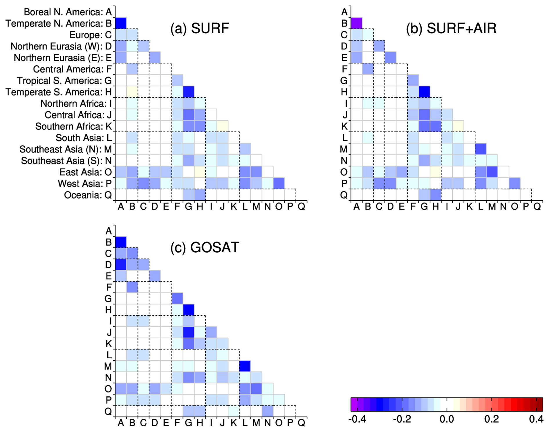
Figure 8 Error correlations of the regionally aggregated posterior fluxes for 2020 (annual mean) in the SURF (a), SURF+AIR (b), and GOSAT (c) inversions. A negative value indicates that estimated fluxes are anti-correlated with each other. The dotted black lines group regions in a broader scale (e.g., Asia for L–P, Eurasia for D and E).

3.4 Sectoral contributions

Although our inversion system does not currently incorporate isotope data to separately evaluate sectoral contributions (Lan et al., 2021; Chandra et al., 2024), we optimized CH₄ emissions by sector with the expectation that spatial and temporal variations of observations could to some extent provide information about sectoral contributions. If different sectors do not overlap with each other in space and time, they might be optimized independently. However, it would largely depend on prior emissions ratios.

Year-to-year variations of the merged sectoral CH₄ fluxes are presented in Fig. 9. For the entire period, the GOSAT inversion estimated larger wetland emissions and smaller fossil fuel emissions than the SURF and SURF+AIR inversions, which reflects the larger emissions in the tropics and the smaller emissions in the northern mid-latitudes (Fig. 3). Nevertheless, their temporal changes are generally consistent with each other. Interestingly, every sector contributed to the increase in CH₄ emissions for 2020–2022 but in different ways. One prominent feature is the increase in wetland and agriculture–waste emissions in 2020 (magnitudes of approximately 15 Tg CH₄ yr⁻¹ for both). Also, fossil fuel emissions are increased in 2020 by ca. 10 Tg CH₄ yr⁻¹, but the previous drop in 2019 is notable. Biomass burning emissions have two peaks in 2019 and 2021 (up to 10 Tg CH₄ yr⁻¹). In 2021, the SURF and SURF+AIR inversions showed a decrease in wetland emissions but more biomass burning emissions in the northern high latitudes. In contrast, the GOSAT inversion estimated a more moderate decrease and increase for each of these, respectively. However, all the inversions agree with the increases in agriculture–waste emissions in the northern low latitudes and in wetland emissions in the tropics, both of which contributed a large part of the global CH₄ emissions increase for 2020–2022.

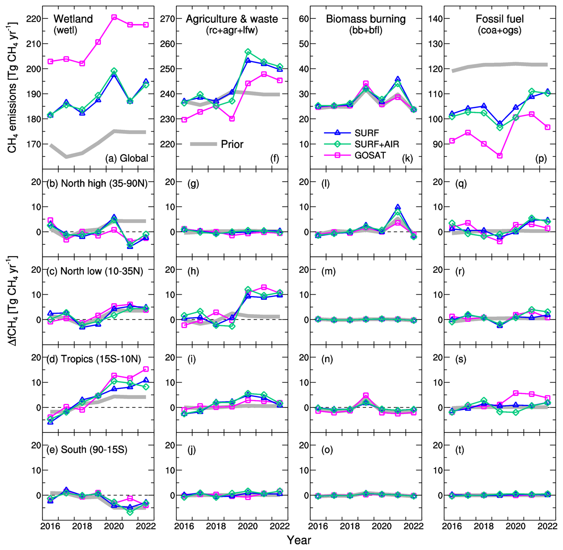
Figure 9 Same as Fig. 5 but separated for sectoral emissions from wetland (wetl) (a–e), agriculture–waste (rc+agr+lfw) (f–j), biomass burning (bb+bfl) (k–o), and fossil fuels (coa+ogs) (p–t). Sectorial emissions are merged as shown in Table 1.

Figure 10 summarizes regional ΔfCH₄ increases for 2020–2022 by four sectors. Only for wetlands are notable increases estimated by the prior data, in which the VISIT data for 2020 were repeatedly used for 2021–2022. The inversions consistently suggested that the emission increases in Tropical South America and northern Southeast Asia were attributable to wetland and agriculture–waste (dominated by rice cultivation in the prior flux), respectively. The inversions also agree that the emission increase in South Asia was from both wetland and agriculture–waste sectors. However, the other emissions are estimated differently by the inversions. Biomass burning emissions are estimated to have increased in Northern Eurasia and Boreal North America by the SURF and SURF+AIR inversions, but the increase is offset by decreases in southern Southeast Asia and other regions. In southern Southeast Asia, the GOSAT inversion estimated larger biomass burning emissions in 2019; however, they diminished in 2020–2022 resulting in the larger decrease in biomass burning ΔfCH₄. For fossil fuel emissions, the GOSAT inversion suggested a large increase in contributions not only from the Asian regions but also from Central Africa (more than 8 Tg CH₄ yr⁻¹ in total). Meanwhile, the SURF and SURF+AIR inversions showed moderate increases of about 4 Tg CH₄ yr⁻¹, which are mostly from East Asia.

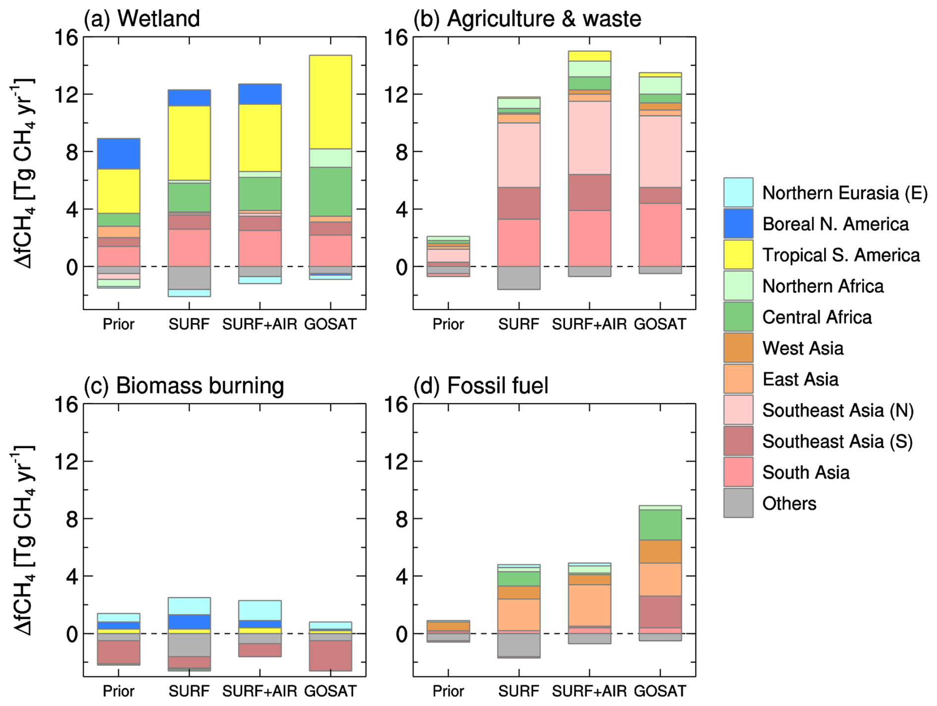
Figure 10 Same as Fig. 7 but separated for sectoral emissions from wetland (wetl) (a), agriculture–waste (rc+agr+lfw) (b), biomass burning (bb+bfl) (c), and fossil fuels (coa+ogs) (d). Sectorial emissions are merged as shown in Table 1.

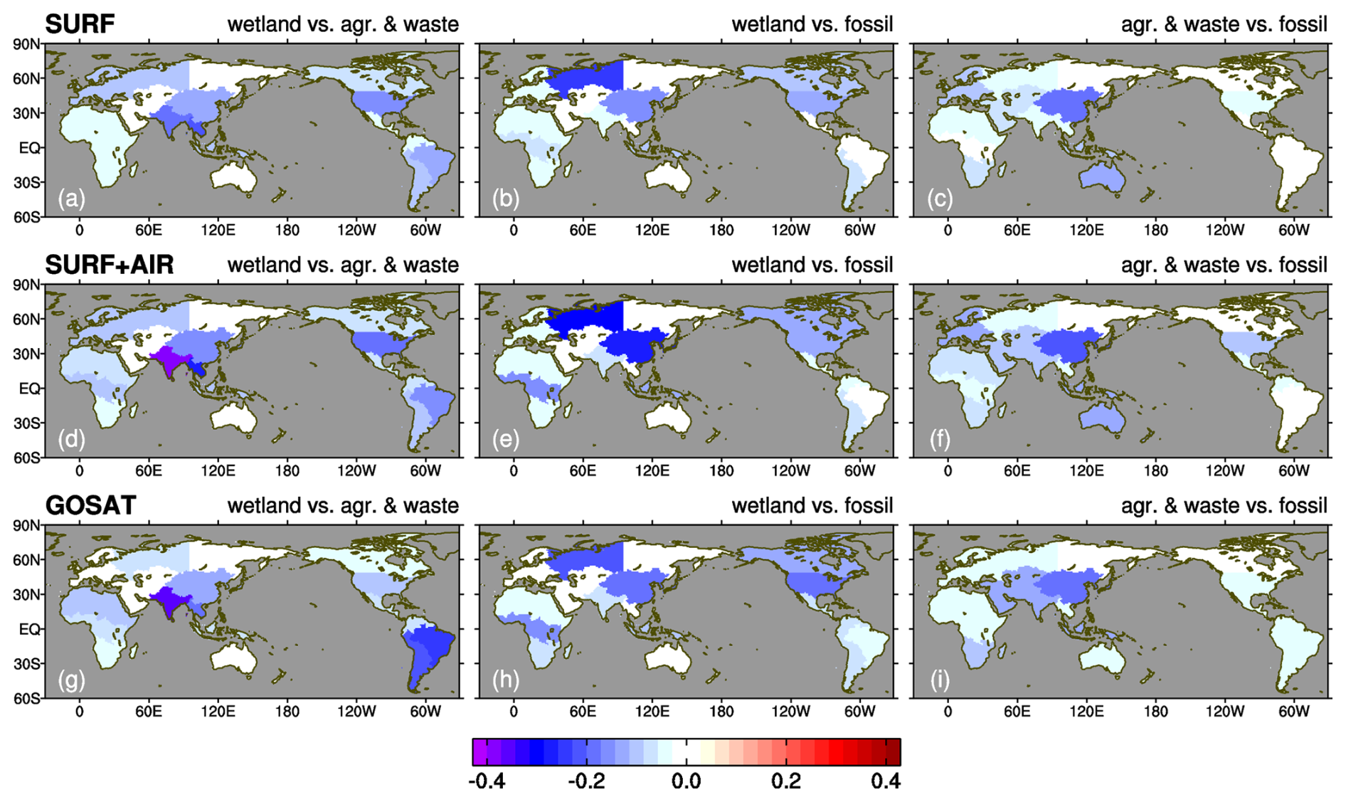
Figure 11 Posterior error correlations between wetland and agriculture-waste emissions (left), wetland and fossil fuel emissions (center), and agriculture–waste and fossil fuel emissions (right) for the SURF (top), SURF+AIR (middle), and GOSAT (bottom) inversions. Error correlations are aggregated for each geographical region (Fig. 6).

The aforementioned sectoral contributions have uncertainties because in many regions, different sectoral emissions overlap or are close enough to well-mixed flux signals in the atmosphere. To assess uncertainties of sectoral contributions, we calculated posterior error correlations among the three major sectors: wetland, agriculture–waste, and fossil fuel emissions. Figure 11 shows the regionally integrated posterior error correlations among the three sectors for the three inversions. South Asia, the biggest contributor to the emissions increase for 2020–2022 (Fig. 7), has the strongest anti-correlation between wetland and agriculture–waste emissions. This anti-correlation is particularly enhanced when aircraft or GOSAT data are used, probably because aircraft and GOSAT observe well-mixed air masses that cannot resolve wetland/agriculture emission signals. Furthermore, the other dominant contributors (northern Southeast Asia and Tropical South America) also have notable anti-correlations between wetland and agriculture–waste emissions. Therefore, the dominant increases in agriculture–waste emissions in northern Southeast Asia and wetland emissions in Tropical South America (Fig. 10) might have some contributions by wetland emissions and agriculture–waste emissions, respectively. Nevertheless, because wetland or agriculture–waste emissions in these areas do not have notable anti-correlations with fossil fuel emissions, we can conclude that biogenic (wetland and/or agriculture–waste) emissions have dominantly contributed to the increase for 2020–2022.

The contribution of wetland emissions in Central Africa is also large (Fig. 10a), and its anti-correlations with the other emissions are small, indicating the robustness of the wetland contribution there. Fossil fuel emissions in East Asia, which have the largest contribution in this sector (Fig. 10d), have notable anti-correlations with wetland and agriculture–waste emissions (Fig. 11e and f), indicating the possibility of contributions from biogenic emissions. Error correlations of fire emissions, which are not shown in Fig. 11, are small compared to the abovementioned ones. A small negative error correlation of −0.2 at most with wetland emissions was found in the east part of Northern Eurasia for the SURF+AIR inversion, while other areas/cases have negligible anti-correlations. This is probably because fires occur in a relatively small area, which makes it easy to separate them from other sector emissions (note that fluxes are optimized at each 1°×1° grid point, not in each aggregated region).

4 Discussion

4.1 OH reduction due to the COVID-19 pandemic

This study investigated the surge of atmospheric CH₄ during 2020–2022 by the inverse analysis with NISMON-CH₄, which assumes that atmospheric OH abundance did not change during this period. However, we recognize that this is an optimistic assumption, especially for 2020. In fact, previous studies have suggested a significant contribution from the OH decrease as a result of the COVID-19 pandemic (Qu et al., 2022; Feng et al., 2023; Stevenson et al., 2022; Peng et al., 2022). Therefore, we performed a sensitivity test by reducing OH and accounting for the pandemic in 2020, although we used a simpler approach compared with other studies that considered atmospheric chemistry reactions with NO_x. Details of the approach are described in Appendix C.

In the sensitivity tests of SURF and GOSAT, total ΔfCH₄ in 2020 was reduced by 17 % and 29 % globally, respectively. Furthermore, those impacts appeared in the northern low-latitude and tropical regions, where notable increases in emissions were found in the control inversions (Fig. C1). In particular, Tropical South America shows the largest emissions reduction of 4 Tg CH₄ yr⁻¹ with the OH reduction. Meanwhile, the OH reduction induced 2–3 Tg CH₄ yr⁻¹ emissions reduction in Central Africa, northern and southern Southeast Asia, and South Asia. However, the reduction of OH we tested in this study is relatively large compared to other studies. Moreover, a recent study suggested much less OH reduction using multiple hydrofluorocarbon observations (Thompson et al., 2024). Therefore, our estimate of the effect of the OH reduction might be overestimated. Even with the reduced OH, northern Southeast Asia, one of the prominent contributors to the atmospheric CH₄ surge, still shows a notable emissions increase from 2019 to 2020. Furthermore, the reduced OH inversion with GOSAT still shows a notable emission increases in South Asia from 2019 to 2020. These results indicate that emissions in northern Southeast Asia and South Asia contributed to the surge of atmospheric CH₄ growth from 2019 to 2020. Given the limited OH reduction for 2021–2022 (Liu et al., 2023; Li et al., 2023), those high emissions continued until 2022.

4.2 Uncertainties in regional estimates

One notable feature of our inversion results is that the biogenic (wetland and agriculture–waste) emissions from Asia are the most important contributor to the increase in atmospheric CH₄ since 2020 (Fig. 7). However, similar inversion studies of Qu et al. (2022) and Feng et al. (2023) suggested a higher contribution from Africa. These previous inversions mainly used GOSAT data that were produced by the proxy method of the University of Leicester (GOSAT-UoL; Parker and Boesch, 2020), which has more data than the NIES GOSAT product (the full-physics method) we used (Fig. D1b). To examine the influence of the different GOSAT products, we performed an additional inversion using the GOSAT-UoL data with the same inversion settings, but the period covered was only through 2021 because of data availability (Appendix D). In this inversion analysis, we obtained a notable increase in ΔfCH₄ in Northern Africa for 2020–2021 as well as in Central Africa for 2020 (Fig. D2). Meanwhile, compared with the GOSAT-NIES inversion, ΔfCH₄ is reduced in East Asia for 2020 and northern Southeast Asia for 2020–2021, though the increase in ΔfCH₄ in South Asia for 2020–2021 is retained or even enhanced for 2020. This result indicates that the increase in CH₄ emissions from Africa suggested by the previous studies is attributable to the use of GOSAT-UoL data, probably because the denser data of GOSAT-UoL have flux signals from Africa that are not represented in GOSAT-NIES, surface, or aircraft data. In fact, as shown by the error reduction ratio in Fig. D2, GOSAT-UoL imposed strong constraints on flux estimates for the African regions. As shown in Fig. 7, the GOSAT-NIES inversion estimated larger emissions in Africa than the SURF and SURF+AIR inversions. Therefore, the larger emission increase from Africa is attributable to GOSAT itself, regardless of the product used. As of now, we cannot conclude which regional emission has made the largest contribution to the atmospheric CH₄ surge since 2020. The error reduction ratios by GOSAT-UoL are larger in the African and Asian regions than those of GOSAT-NIES (Fig. D2), but they are calculated under the assumption that observations are not biased. In fact, the full-physics method and the proxy method could have non-negligible differences in retrieved XCH₄ data (Schepers et al., 2012). For evaluating these satellite products differences, we need to expand in situ or flask observation networks, especially in the African regions; this would also be useful to investigate notable differences of atmospheric CH₄ between GOSAT and flask observations found in the tropics and southern latitudes (Fig. B1; similar differences are also found between GOSAT-UoL and flask observations (not shown)).

Meanwhile, Appendix D also highlights the importance of emissions from the Asian regions, using unique surface observations from NIES, which include ground-based flask samplings in the Asian countries (India, Bangladesh, and Malaysia) (Nomura et al., 2021) and ship measurements in the western Pacific and around Southeast Asia (Terao et al., 2011; Nara et al., 2017). In fact, these observations provided greater confidence in flux estimates in the Asian regions by providing stronger observational constraints (Fig. D2). Although omitting the NIES observations did not largely change the general features of the ΔfCH₄ changes, Fig. D2 shows that the increase in 2021 was clearly attributed to the use of the NIES observations. Furthermore, as shown by Fig. 6, aircraft data (which were uniquely used in the inversion in this study) supported the large emissions increase from the Asian regions with additional strong constraints. The effectiveness of aircraft data in constraining the estimates is attributable to active vertical transport, which is typical in these regions (i.e., the summer monsoon) (Niwa et al., 2012, 2014, 2021).

4.3 Sectoral contributions

Whether from Africa or Asia, our inversions agree with previous inversions in that biogenic emissions dominated the probable increase in CH₄ emissions. This large biogenic emission contribution is consistent with other studies that use the stable CH₄ isotope (δ¹³CH₄) measurements (Nisbet et al., 2023; Chandra et al., 2024). The expanded area of inundation, which is probably related to the prolonged La Niña during 2020–2022, might have increased biogenic emissions in the northern low-latitude areas (Feng et al., 2023; Lin et al. 2024). Detailed analyses on these sectoral contributions by comparing them with meteorological parameters would provide insights into CH₄ emissions mechanisms. To this end, including the year of 2023 in the analysis period would be beneficial because the climate changed from La Niña to El Niño conditions in 2023. In fact, the growth rate of atmospheric CH₄ seems to have decreased in 2023 (Lan et al., 2024). Furthermore, using observations of the stable CH₄ isotope would also be beneficial (Lan et al., 2021; Chandra et al., 2024). Additional analyses focusing on these climate condition changes are left for a future study.

Following those biogenic emissions, the inversions suggested increases in fossil fuel emissions, especially from Asian regions and Central Africa (Fig. 10). However, they were largely contributed by the recovery from the drop in 2019 (Fig. 9), whose cause is unclear at this moment. Furthermore, the increase in the fossil fuel emissions for 2020–2022 could be partly contributed by misallocation of biogenic emissions because East Asia, which is the largest contributor of this sector (Fig. 10), has anti-correlations between fossil fuel emissions and wetland and agriculture–waste emissions (Fig. 11).

The SURF and SURF+AIR inversions also suggested emission increases in the northern high latitudes from wetlands for 2020 (ca. 5 Tg CH₄ yr⁻¹) and from biomass burnings for 2021 (ca. 9 Tg CH₄ yr⁻¹) (Figs. 9 and 10). They can probably be attributed to the Siberian heat wave in 2020 (Overland and Wang, 2021) and the boreal fires in 2021 (Zheng et al., 2023), respectively. In fact, even though these emission increases are large enough to note, the decrease in wetland emissions in 2021 makes the contribution of the northern high latitudes to the 2020–2022 surge minor (Fig. 7). Meanwhile, the GOSAT inversion did not clearly reproduce emission increases in the northern high latitudes, and this difference should be investigated in a future study.

5 Conclusions

This study used the inversion method with multiple observational datasets to estimate probable emission increases that induced the latest record-breaking surge of atmospheric CH₄ in 2020–2022. Using three different observational datasets (SURF, SURF+AIR, and GOSAT), this study suggested that emissions in the tropics and the northern low-latitude areas notably increased by 10–18 and 20 Tg CH₄ yr⁻¹, respectively, from 2016–2019 to 2020–2022. Specifically, the inversions consistently estimated notable emission increases in Tropical South America (5–7 Tg CH₄ yr⁻¹), Central Africa (3–6 Tg CH₄ yr⁻¹), South Asia (6–7 Tg CH₄ yr⁻¹), and northern Southeast Asia (5 Tg CH₄ yr⁻¹). The emissions in Tropical South America and Central Africa showed gradual persistent increases for the analysis period (2016–2022), and they are mostly attributable to wetlands. The results also indicated that the two Asian regions (South Asia and northern Southeast Asia) contributed to the surge of atmospheric CH₄ with the sharp annual rise in their emissions from 2019 to 2020, and the elevated emissions continued until 2022. For these two regions, wetland and agriculture–waste sectors were estimated to be the largest contributors to the increased emissions for the period, although notable anti-correlations of the posterior errors indicate that relative contributions from these two regions or these two sectors remain underdetermined. Given that changes of anthropogenic emissions are slow, it seems likely that wetlands were the main driver of the emission growth. However, for either the prior or posterior data, rice cultivation emissions are the largest in northern Southeast Asia (approximately twice as large as wetland emissions) and comparable to wetland emissions in South Asia; a growth of such anthropogenic emissions cannot be denied, and it would suggest a potential impact of direct emissions reduction measures on this sector for these two Asian regions.

The above inversion results are reliable for several reasons: (1) the spatiotemporal variations of posterior atmospheric CH₄ mole fractions are improved from the prior ones in comparison with multiple observations, and (2) the inversions with independent observations (SURF(or SURF+AIR) and GOSAT) agree in finding that biogenic emissions in the tropics and northern low latitudes are the main contributors to the emissions increases. The flux estimates for the Asian regions are particularly noteworthy because the probable reduction of OH resulting from the pandemic-derived lockdown would not have largely affected the flux estimates in Asia, as suggested by the sensitivity test results. Furthermore, the dense observation network including not only surface observations but also ship and aircraft observations, which was newly introduced in this study, provided strong constraints and increased the confidence in the Asian flux estimates.

Other studies using the GOSAT proxy method data suggested the predominant role of emission increases in Africa. The results of this study cannot deny Africa as a possible source of the emissions increase, but they give prominence to the biogenic emissions in South Asia and northern Southeast Asia for the surge of atmospheric CH₄ from 2019 to 2020–2022. To evaluate those different satellite-based estimates, we need more elaborate networks of high-precision in situ and flask observations not only at the surface but also in the upper air (by aircraft); these observations are especially needed in the tropical and low-latitude areas of Africa, South America, and Asia.

Appendix A: Exterior penalty function method to avoid negative fluxes

Surface CH₄ fluxes from each sector are mostly one way; that is, fluxes other than soil uptakes are all positive (from the surface to the atmosphere), and soil uptake fluxes are all negative (from the atmosphere to the surface). In fact, this is also true for the prior flux data. However, it is not the case for posterior fluxes because scaling factors or flux deviations optimized through inversion may induce unrealistic negative fluxes (and positive ones for soil uptakes). To avoid such unrealistic fluxes, CH₄ inversions often use a numerical technique. For instance, Bergamaschi et al. (2009) transformed control variables with a “semiexponential” function.

In NISMON-CH₄, we use the exterior penalty function method (Sawada and Honda, 2021), which introduces an additional constraint with a so-called “penalty term” in the cost function. This penalty term J_p is defined as

$$\begin{array}{}\text{(A1)}& J_{\mathrm{p}}\left(\mathit{x}\right)=\mathit{\lambda }\sum _n\sum _i{\left[\max \left\{\mathrm{0},-f_{n,i}\left({\mathbf{x}}_n\right)\right\}\right]}^{\mathit{\alpha }},\end{array}$$

where x is the control variable vector (i.e., scaling factors and flux deviations), and the indices n and i represent each flux sector and grid point, respectively. The flux operator f_n,i calculates a flux value of the nth sector at the ith grid point from the control variables defined by each term of the right-hand side of Eq. (1) (note that the minus before f_n,i is omitted for soil uptakes to invert the sign). Combined with the conventionally defined cost function J (similar to Eq. 1 of Niwa et al., 2022), this penalty term J_p leads to a constrained optimization problem (negative fluxes are avoided) as

$$\begin{array}{}\text{(A2)}& J_{\mathrm{c}}=J+J_{\mathrm{p}},\end{array}$$

which is used as the cost function in the 4D-Var iterative calculation instead of J. Because negative fluxes make the cost function extremely large, they are avoided in the optimal state, where the cost function reaches the minimum. In this study, the arbitrary parameters of λ and α in Eq. (A1) were set to 1000 and 2, respectively, which were determined according to results of practical optimization trials in terms of computational stability. In fact, this scheme cannot avoid negative values perfectly, but unavoidably generated negative values were at most 3 orders of magnitude smaller than positive values in the experiments.

Appendix B: Mean differences between observed and modeled atmospheric CH₄

Here, we demonstrate how the modeled mole fractions of atmospheric CH₄ are consistent with observations before and after the inversions. Figure B1 shows mean differences between observed and modeled atmospheric CH₄ for surface, aircraft, and GOSAT observations for 2020–2022. These data are the same as those used in Fig. 2, but the offsets (the averages for 2016–2019) are not subtracted; that is, a more direct comparison is conducted here. In general, the SURF, SURF+AIR, and GOSAT inversions are most consistent with the surface, aircraft, and GOSAT observations, respectively. This is not surprising, but it demonstrates that each inversion succeeded in optimizing atmospheric mole fractions as well as fluxes consistently with observations. However, when compared with independent observations, the inversions do not necessarily produce a better agreement with the observations than the prior fluxes do. This is attributable to errors in atmospheric transport, in chemical loss by OH, or in the measurements themselves. The persistent deviations of the GOSAT inversion from the surface observations are especially noticeable in the tropics and the southern latitudes (Fig. B1a), which can also be seen to a lesser extent in the comparison with the aircraft observations (Fig. B1b). Those differences consistently existing at the surface and in the free troposphere may not be contributed by vertical transport or chemical loss in the model. Given that in situ and flask observations have much higher precision than satellite observations, this result indicates that the GOSAT observations have measurable biases in those latitudes. Meanwhile, the SURF and SURF+AIR inversions largely deviate from the GOSAT observations in the tropics and southern latitudes (Fig. B1c), which is consistent with the GOSAT inversion results.

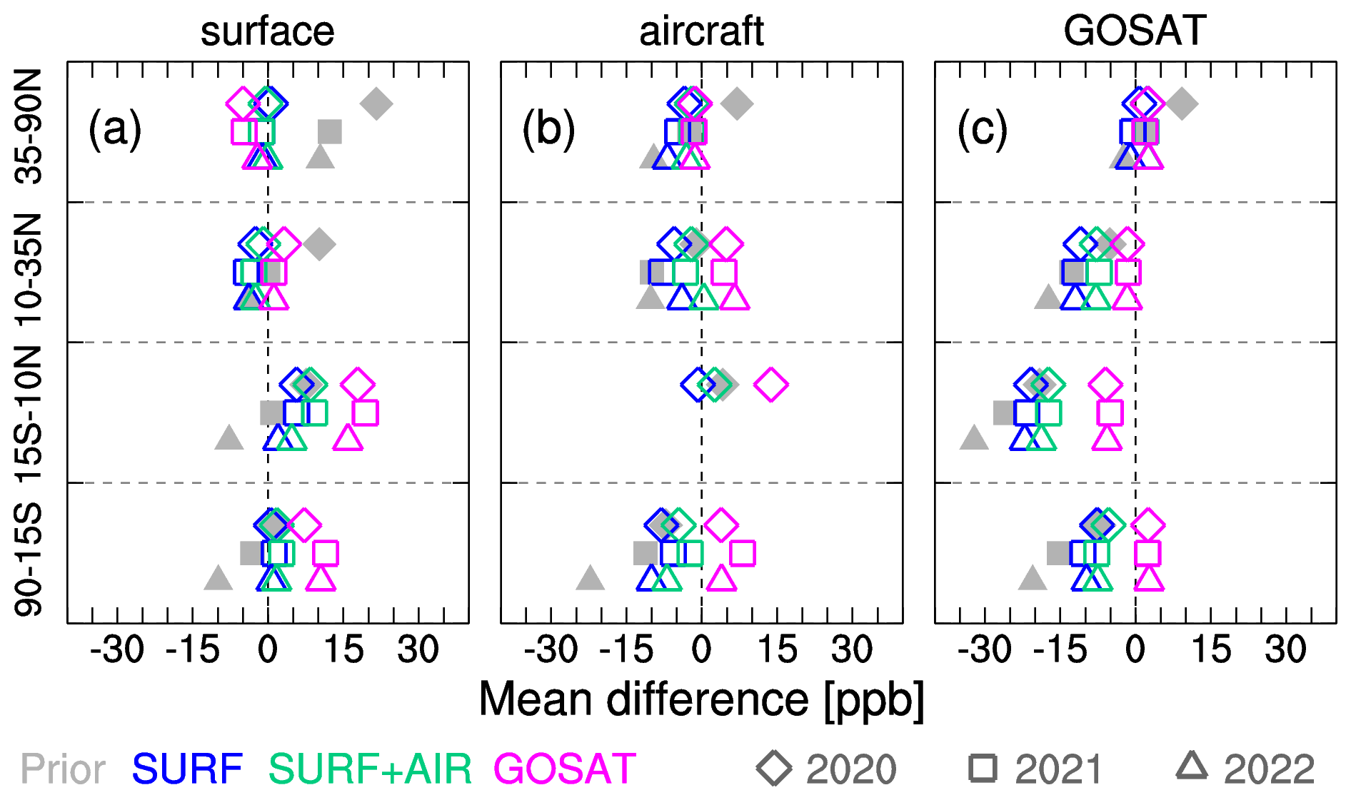
Figure B1 Mean differences between observations and prior or posterior mole fractions of atmospheric CH₄ in northern high latitudes (35–90° N), northern low latitudes (10–35° N), tropics (15° S–10° N), and southern latitudes (90–15° S) for 2020 (diamond), 2021 (square), and 2022 (triangle). The mean differences are calculated for different observational types of surface (a) and aircraft (b) flask observations and for the GOSAT data (c). The prior and posterior mole fractions are derived from atmospheric simulations of NICAM-TM with the prior (gray) and posterior fluxes: SURF (blue), SURF+AIR (light green), and GOSAT (magenta), respectively.

Appendix C: Inversions with reduced OH in 2020

To investigate the probable OH reduction resulting from the COVID-19 pandemic in 2020, we performed sensitivity tests for the SURF and GOSAT inversions. In these tests, we reduced the climatological OH data that were used in the control inversions according to the reduction of fossil fuel CO₂ emissions in 2020. Specifically, we used the fossil fuel CO₂ emissions from the gridded fossil emissions dataset (GridFED; Jones et al., 2021) and calculated their reduction ratios from 2019 to 2020 for each month and grid. Then, each calculated reduction ratio was applied to the OH field over the same grid below the 12th model layer (approximately 3 km above ground level), assuming that the reduction of NO_x emissions and the consequent reduction of atmospheric OH occurred within the surface mixed layer at the same rate as that of CO₂ emissions. The global average of the resulting OH field is smaller by a maximum of 4 % in May than that of the climatological average, and the annually averaged reduction ratio is 2.5 %. This assumed OH reduction is larger than that of Peng et al. (2022) (1.6 %) and Qu et al. (2022) (1.2 %), but it is similar to that of Miyazaki et al. (2021) (4 % in May at a maximum). For the years other than 2020, we used the same climatological OH field.

Figure C1 shows the same regional ΔfCH₄ changes as Fig. 5 but for the additional inversions with the reduced OH. Globally, total ΔfCH₄ in 2020 decreased by 17 % and 29 % for the SURF and GOSAT inversions, respectively. The boreal northern regions, which have less OH, are negligibly affected by the OH reduction for both inversions (SURF and GOSAT). Meanwhile, estimated emissions were reduced in temperate and tropical areas. In Tropical South America, the reduced OH induced the largest emissions reduction (approximately 4 Tg CH₄ yr⁻¹ for both inversions), producing a notable drop from the years before and after the inversions. In addition, the GOSAT inversion estimated smaller emissions by 3 Tg CH₄ yr⁻¹ for southern Southeast Asia and Central Africa and by 2 Tg CH₄ yr⁻¹ for Temperate North America and northern Southeast Asia. Meanwhile, the SURF inversion estimated smaller emissions by 2 Tg CH₄ yr⁻¹ for Central Africa, West Asia, and South Asia. However, even with the OH reduction, northern Southeast Asia still shows a pronounced increase from 2019 to 2020. For South Asia emissions, SURF shows a marginal increase, but GOSAT still shows a large increase from 2019 to 2020.

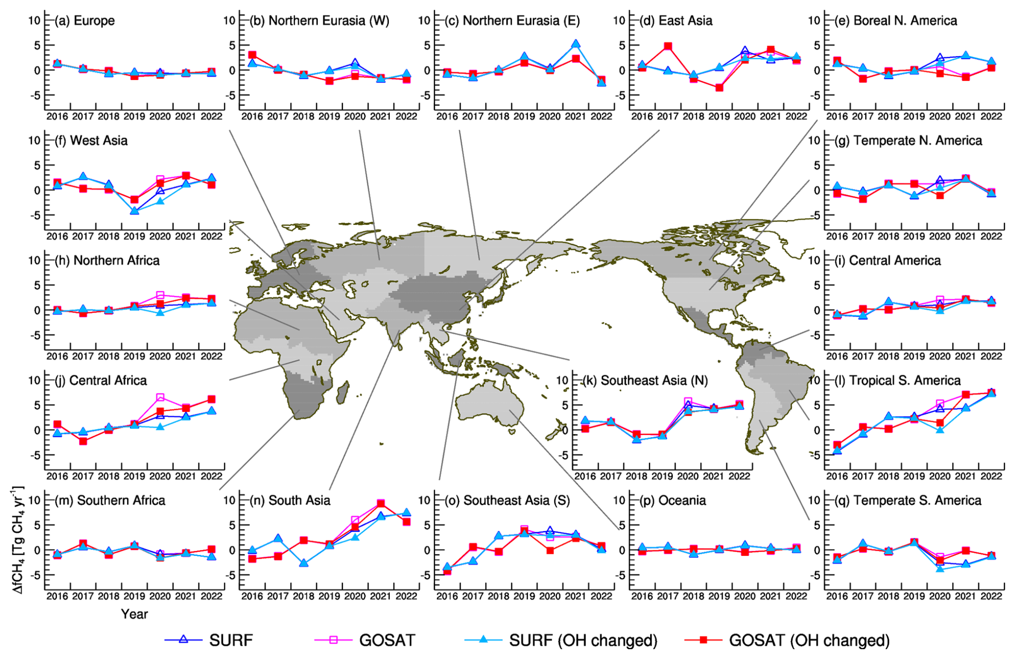
Figure C1 Same as Fig. 6 but including the sensitivity tests with OH reduced in 2020 for the surface (light-blue closed triangles) and GOSAT (red closed squares) inversions.

Appendix D: Inversions without the NIES observations and with the University of Leicester GOSAT proxy data

We performed two additional inversions using different observational networks. One uses the same surface observations but excludes the NIES observations (SURF without NIES; Fig. D1a). The NIES observation network includes flask samplings in South and Southeast Asia, ship measurements in the Asia-Pacific regions, and in situ measurements using towers in Siberia, but those NIES data (except for Siberian) are not included in NOAA GLOBALVIEWplus, which is a major dataset used in other inversion studies, which is a major difference between our study and the others. The second inversion employed the University of Leicester (UoL) version 9.0 GOSAT proxy data (Parker and Boesch, 2020) (GOSAT-UoL) (Fig. D1b).

In this study, we used the NIES GOSAT product, which is produced by the full-physics retrieval method (Yoshida et al., 2011, 2013). Meanwhile, the proxy data are produced by a method that uses modeled CO₂ mole fractions as a proxy to retrieve XCH₄, which is less affected by aerosols and clouds. As shown by Fig. D1b, there are more data available with the proxy method than with the full-physics method (Fig. 1c), particularly for Africa and South America. At the time of this study, the GOSAT-UoL data were available through the end of 2021. Therefore, the inversion with GOSAT-UoL was performed for the period until 2021.

Figure D2 shows the same temporal patterns of ΔfCH₄ for each region as Fig. 5, but the additional inversion results are presented. In general, the additional inversions of SURF without NIES and GOSAT-UoL show temporal variations similar to those of the corresponding control inversions, although there are notable differences in some regions. The SURF without NIES inversion estimated smaller ΔfCH₄ increases in northern Southeast Asia and South Asia for 2021, but it still showed elevated ΔfCH₄ in 2020 and 2022. Compared to the GOSAT inversion, the GOSAT-UoL inversion shows remarkably large ΔfCH₄ increases in Northern Africa for 2020 and 2021, with smaller ΔfCH₄ in East Asia and northern Southeast Asia. The observational constraint (represented by the error reduction ratio) is also different from the original inversion. The SURF without NIES inversion shows weaker observational constraints than those of SURF in the Asia and Oceania regions, indicating that the NIES observations have strong constraints in flux estimates for these regions. Meanwhile, the GOSAT-UoL inversion shows stronger observational constraints than the GOSAT inversion everywhere, and this is more pronounced in the tropical regions (almost doubled). These stronger constraints are attributed to the larger number of data in GOSAT-UoL (Fig. D1b).

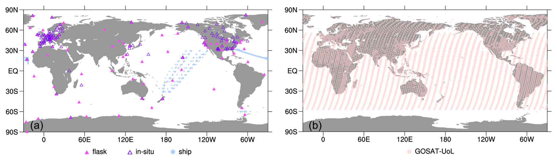
Figure D1 Same as Fig. 1a, but the NIES observations are excluded (a). The GOSAT proxy data from the University of Leicester obtained during 2020 (b).

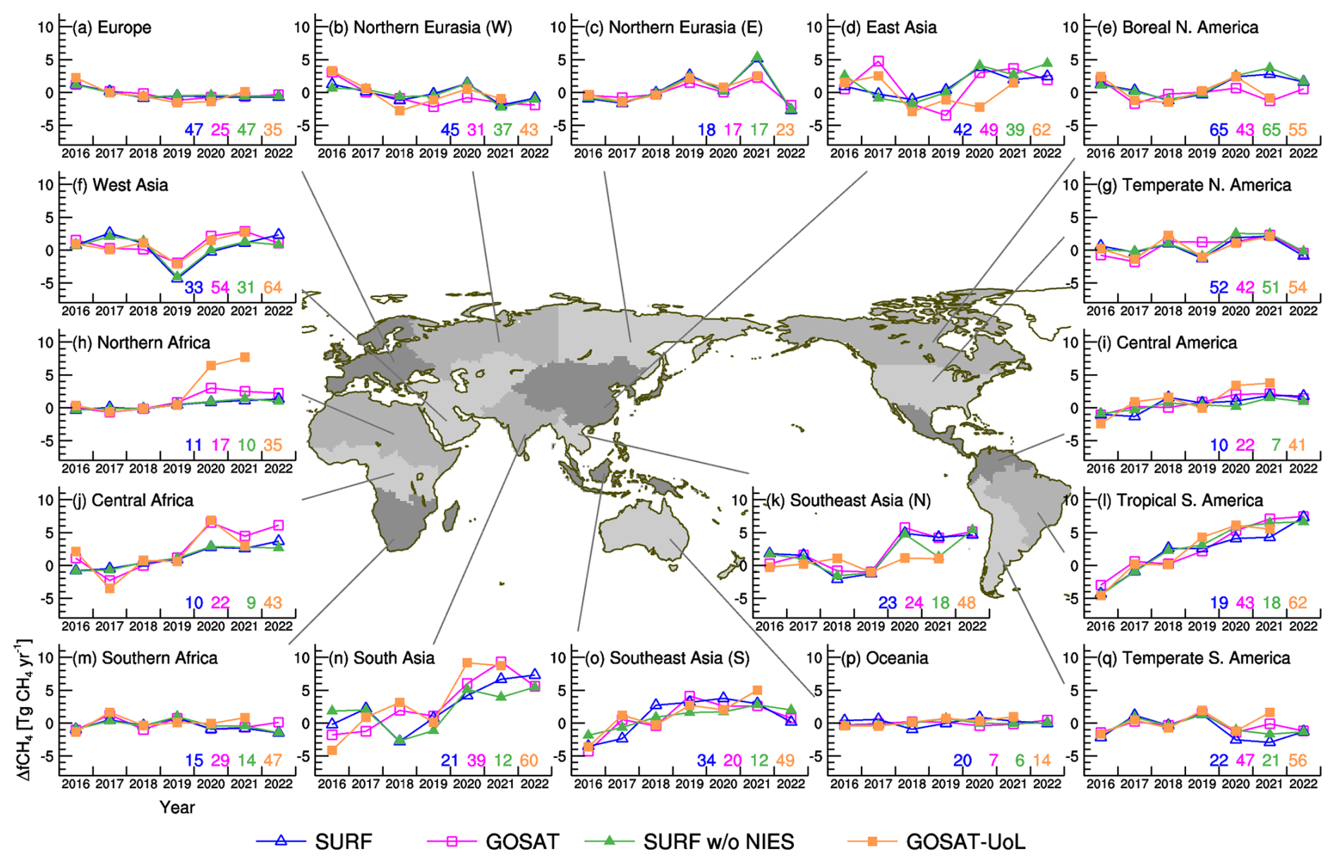
Figure D2 Same as Fig. 6, but the additional inversions using surface observations excluding the NIES observations (green closed triangles) and using the University of Leicester (UoL) GOSAT proxy data (orange closed squares) are shown. Numbers in each panel denote error reduction ratios.