Evaluating spatiotemporal variations and exposure risk of ground-level ozone concentrations across China from 2000 to 2020 using high-resolution satellite-derived data

Understanding the spatial and temporal characteristics of both long- and short-term exposure to ground-level ozone is crucial for refining environmental management and improving health studies. However, such studies have been constrained by the availability of high-resolution spatiotemporal data. To address this gap, we characterized ground-level ozone variations and exposure risks across multiple spatial (pixel, county, region, and national) and temporal (daily, monthly, seasonal, and annual) scales using daily 1 km ozone data from 2000 to 2020, derived from satellite-sourced land surface temperature data via a machine-learning hindcast method. The model provided reliable estimates, validated through rigorous cross-validation and direct comparison with external ground-level ozone measurements. Our long-term estimates revealed seasonal shifts in high-exposure ozone centers: spring in eastern China, summer in the North China Plain (NCP), and autumn in the Pearl River Delta (PRD). A non-monotonic trend was observed, with ozone levels rising from 2001–2007 at a rate of 0.47 $\mathrm{\mu }\mathrm{g}{\mathrm{m}}^{-\mathrm{3}}{\mathrm{yr}}^{-\mathrm{1}}$, declining after 2008 (−0.58 $\mathrm{\mu }\mathrm{g}{\mathrm{m}}^{-\mathrm{3}}{\mathrm{yr}}^{-\mathrm{1}}$), and increasing significantly from 2016–2020 (1.16 $\mathrm{\mu }\mathrm{g}{\mathrm{m}}^{-\mathrm{3}}{\mathrm{yr}}^{-\mathrm{1}}$), accompanied by regional and seasonal fluctuations. Notably, ozone levels increased by 0.63 $\mathrm{\mu }\mathrm{g}{\mathrm{m}}^{-\mathrm{3}}{\mathrm{yr}}^{-\mathrm{1}}$ in summer in the NCP during the second phase and by 6.38 $\mathrm{\mu }\mathrm{g}{\mathrm{m}}^{-\mathrm{3}}{\mathrm{yr}}^{-\mathrm{1}}$ in autumn in the PRD during the third phase. Exposure levels over 100 µg m⁻³ have shifted from June to May, and levels exceeding 160 µg m⁻³ were primarily seen in the NCP, showing an expanding trend. Our day-to-day analysis highlights the influence of meteorological factors on extreme events. These findings emphasize the need for increased public health awareness and stronger mitigation efforts.

1 Introduction

Ground-level ozone is a critical pollutant and greenhouse gas in the atmosphere. A growing body of research has demonstrated that both short-term and long-term exposure to ambient ozone are linked to various adverse health outcomes, including asthma (Nicholas et al., 2020), respiratory tract infections (Burnett et al., 1994), and even premature deaths (Maji and Namdeo, 2021). Moreover, severe ozone pollution in the ambient environment also impacts agricultural crops and contributes to climate change (Li et al., 2018; Ramya et al., 2023). Therefore, it is crucial to investigate the long-term variation in ground-level ozone, especially for China, a country undergoing significant atmospheric environmental changes due to its rapid economic growth and evolving air pollution control policies over the last 2 decades. Additionally, influenced by a mix of meteorological conditions, local emissions, and regional transport mechanisms (Fiore et al., 2003; Jaffe, 2011; Monks et al., 2015), ground-level ozone exhibits considerable heterogeneities in its spatial distribution and temporal trends. Understanding these fine-scale variations can provide more precise information about local ozone variations, for example, information to identify local ozone spikes (Shi et al., 2023; Chen et al., 2022) and to enable accurate assessments of human exposure to ozone at the community or even neighborhood level (Alexeeff et al., 2018). However, such intricate tasks cannot be accomplished solely by the ground-level air quality monitoring network. While monitoring networks offer accurate ozone concentration data, their limited observation duration and sparse station distribution inadequately capture intraurban variations, often resulting in underestimates of neighborhood and individual exposure variability (Dias and Tchepel, 2018). Therefore, it is necessary to enhance the understanding of ground-level ozone variation and enable more effective mitigation measures using full-coverage, long-term ozone data with high spatiotemporal resolution.

To date, various methods have been employed to address the limitations of ground-level ozone data for a more comprehensive understanding. Atmospheric chemical transport models (CTMs) have been extensively used to simulate ground-level ozone concentrations (Sharma et al., 2017). However, this method typically provides coarse-resolution simulations (usually ≥ 12 km × 12 km) (Qiao et al., 2019; Sun et al., 2019). Due to the large uncertainty in the emission inventory, many assumptions are made when running the CTM, which also incurs high computational costs (Sharma et al., 2017). Advanced statistical and machine-learning algorithms provide an alternative way to obtain spatiotemporal patterns in ozone. By combining with ground-level ozone observations and satellite-retrieved columnar ozone and/or precursor data, those machine-learning methods have significantly improved estimation accuracies (e.g., validated R² values higher than 0.80) and refined the spatial resolution of the estimates (e.g., 0.1° × 0.1° and 0.05° × 0.05°) (Zhang et al., 2020; Mu et al., 2023b; Li and Cheng, 2021; Li et al., 2020; Mu et al., 2023a; Zhu et al., 2022; Xue et al., 2020; Chen et al., 2021). Given that the variation in ground-level ozone is influenced by atmospheric and geographic factors (Wang et al., 2022b; Tu et al., 2007; Zhu et al., 2022; Li et al., 2019; Fu and Tai, 2015), several studies have employed statistical and machine-learning algorithms using atmospheric components (e.g., PM_2.5), meteorological factors (e.g., temperature, wind, sunshine, and precipitation), and relatively high-resolution surface conditions (e.g., elevation and land cover) data as predictors for modeling. While previous studies have estimated ground-level ozone concentrations across China with improved estimation performance (Ma et al., 2022a; Liu et al., 2020; Zhan et al., 2018; Chen et al., 2021; Wei et al., 2022; Shang et al., 2024), at least two key limitations persist. The first limitation is as follows: (1) despite advancements in resolution technology, these studies have not achieved high resolution in both spatial and temporal dimensions, such as daily 1 km estimates. This shortfall is partly due to the limited incorporation of suitable high-resolution spatiotemporal proxies into the models, which are essential for capturing fine-scale ozone gradients across space and time. The second limitation is as follows: (2) although gap-free ozone estimates have been provided, few studies track long-term variations before 2005, and even fewer offer external or independent validation for pre-2013 estimates when national air quality monitoring data were unavailable. Consequently, the current datasets are either insufficiently detailed or validated to detect fine-scale intra- and inter-city ozone variations over time, thereby limiting the accuracy of exposure assessments.

Ozone is a short-lived pollutant, exhibiting significant spatial and temporal variations even over small areas and short periods (Mukherjee et al., 2018; Shi et al., 2023). The scarcity of long-term, spatiotemporally detailed ozone data has historically confined ozone research to identifying exposure hotspots and events from a broad-scale or a time-aggregated perspective (Liu et al., 2022; Mashat et al., 2020; Xia et al., 2022). The detailed intraurban differences and short-duration phenomena over the past 2 decades remain largely unexplored. To address this gap, our study utilizes a long-term ground-level ozone concentration dataset across China from 2000 to 2020 with daily 0.01° (∼1 km) spatiotemporal resolution. This dataset is used to evaluate general spatial patterns of long-term ozone variations, identify hotspots of population exposure to ground-level ozone across multiple spatial and temporal scales, and examine the implications for mitigation policies and public health. The ozone dataset is estimated using our previously developed spatiotemporal high-resolution machine-learning-based ozone estimation framework, which incorporates land surface temperature (LST), derived from long-term, high-resolution satellite remote sensing observations, as a primary predictor (He et al., 2024). To ensure the reliability of the long-term exposure analysis, the estimates were evaluated through rigorous cross-validation and independently validated using external ozone measurements. The exposure analysis integrates these high-resolution ozone estimates with detailed population distributions derived from geographic big data.

2 Data and methodology

2.1 Long-term ozone estimates and validation

The present study builds on our previously developed high-resolution ozone modeling framework to hindcast long-term ozone concentration data across China from 2000 to 2020. That framework was designed to predict the daily maximum 8 h average (MDA8) ozone concentrations at a 0.01° spatiotemporal resolution using the extreme gradient-boosting (XGBoost) algorithm. It incorporated four groups of predictors: meteorological parameters (e.g., land surface temperature (LST), boundary layer height), pollutant variables (e.g., nitrogen dioxide, aerosol optical depth), geographical covariates (e.g., elevation, land cover classification), and temporal dummy variables (e.g., day of the year). In that model, satellite-derived LST data, with full coverage and daily 0.01° resolution, served as the primary predictor. Since the data sources, preprocessing approaches, and predictor selection for the current long-term hindcast estimation model closely follow the previously developed modeling framework, further details are documented in Sect. S1 in the Supplement.

The model development process closely mirrors that of our previous high-resolution model. The XGBoost algorithm (Chen and Guestrin, 2016) is also utilized to train the long-term hindcast model due to its demonstrated effectiveness in ground-level ozone estimation at an acceptable computational cost, as indicated by our previous study (Li et al., 2024b). Given that the Chinese National Air Quality Monitoring Network (NAQMN) was not established before 2013, and monitoring data from that period are unavailable, we apply a widely used pre-2013 PM_2.5 hindcast-modeling approach to predict long-term ozone concentrations (Ma et al., 2022b). Specifically, we train the ozone estimation model on data from 2014 to 2020, and once the model is adequately trained, we apply it to retrospectively predict ozone concentrations for the past 2 decades, including the 14 years preceding the establishment of the NAQMN. The study period is partitioned following the approach of a previous study (Zhu et al., 2022), with 2014–2020 as the training period and 2000–2013 as the hindcast period. We exclude the year 2013 from our hindcast modeling due to the limited number and data quality of air quality monitoring stations during NAQMN's inaugural year. We focus on optimizing four critical hyperparameters of XGBoost to balance model performance and computational efficiency: (1) n_estimators, the number of trees in the model; (2) max_depth, which controls the maximum tree depth to prevent overfitting; (3) colsample_bytree, the proportion of features sampled for each tree; and (4) min_child_weight, the minimum number of samples required in a child node. We employ a random search with cross-validation to find the optimal settings for these hyperparameters, which are set at 400, 14, 0.8, and 4, respectively. This hyperparameter setting is a trade-off between model performance and the computational demand. We implemented the modeling process in Python (ver. 3.9) with the Sklearn XGBoost package (ver. 1.7.3).

Due to the absence of nationwide ground-level ozone measurements prior to 2013, directly assessing the estimates for those years is challenging. To address this, we employ the leave-1-year-out cross-validation (CV) method to evaluate the reliability of our long-term hindcast model in estimating years without ground-level ozone measurements. This approach involves withholding data from 1 entire year during model training, simulating a hindcast scenario where ozone measurements are unavailable. This state-of-the-art evaluation technique is widely used in PM_2.5 hindcast modeling for pre-2013 predictions (Ma et al., 2022b). Additionally, although limited, some ground-level ozone measurements from before 2013 are available from monitoring sites in Hong Kong SAR (Hong Kong hereafter). To further validate the pre-2013 predictions, we use these independent Hong Kong ozone measurements – excluded from model development – to directly assess the model's performance during the extended historical period. This provides a more straightforward evaluation, given the lack of nationwide pre-2013 ozone data. In addition to validating hindcast predictions for the pre-2013 period, we also apply the random 10-fold CV to assess the overall performance of our model. This process involves randomly dividing the sample dataset into 10 subsets, using nine subsets to train the model and the remaining subset to test it. This procedure is repeated 10 times to ensure that each daily MDA8 measurement has a corresponding estimate for comparison. The site- and day-based CVs specifically assess the model's spatial and temporal performance. We compute several statistical metrics, including R², RMSE (root-mean-square error), and MAE (mean absolute error), to compare the MDA8 measurements with the model estimates.

2.2 Multi-scale spatiotemporal analysis

We generated full-coverage, daily 1 km resolution ozone estimates across China from 2000 to 2020 using the proposed hindcast machine-learning method. Based on these long-term, high-resolution spatiotemporal estimates, we analyzed interannual, seasonal, and monthly variations, as well as short-term exposure characteristics, at national, regional, county, and pixel scales. Particular attention was given to typical high-exposure regions, which were identified by mapping the spatial distributions of seasonal averages across the study areas over the past 2 decades.

2.2.1 Long-term trend analysis

To assess long-term exposure trends, we combined the MDA8 ozone estimates with concurrent yearly 1 km LandScan population distributions (Rose et al., 2020) to compute the annual and seasonal population-weighted mean MDA8 ozone concentrations for China and typical regional hotspots from 2000 to 2020. These population-weighted concentrations were used to analyze interannual variations, seasonal fluctuations, and regional differences in long-term ozone trends at both national and regional levels. The four seasons were defined as follows: spring (March–May), summer (June–August), autumn (September–November), and winter (December–February). The detailed formulation for calculating population-weighted ozone levels (O₃_POP) for a given region is presented in Eq. (1). The long-term linear trend was estimated using the least-squares approach, consistent with previous studies (Li et al., 2019; He et al., 2016).

$$\begin{array}{}\text{(1)}& {\mathrm{O}}_{\mathrm{3}}\mathit{\_}\text{POP}=\sum ({\text{POP}}_i\times {\text{O}}_{{\text{3}}_i})/\sum {\text{POP}}_i,\end{array}$$

where POP_i and ${\text{O}}_{{\text{3}}_i}$ denote the population and the estimated MDA8 O₃ level in grid cell i, respectively.

2.2.2 Monthly pattern analysis

We calculated the monthly population-weighted mean MDA8 ozone concentrations, from 2000 to 2020, and identified the peak and trough values from these monthly time series. To capture both seasonal extremes and the underlying background ozone concentrations, we calculated linear trends separately for the peaks and troughs. Additionally, we applied a Mann–Kendall test to the monthly peak time series to determine whether there is a statistically significant trend in maximum ozone concentrations over the 2 decades for various regions in China. To assess the extent of severe ozone pollution across counties over time, we generated time series data on the counties with monthly ozone concentrations exceeding 100 µg m⁻³ and analyzed the linear trend. The threshold of 100 µg m⁻³ was selected based on the Chinese National Air Quality Standard Level 2 and the WHO (World Health Organization) air quality guideline value as an indicator of severe exposure. From the monthly exposure time series, we selected a month with severe ozone pollution to map the spatial disparity in ozone exposure at the county level.

2.2.3 Short-term characteristics analysis

By overlaying the daily ozone estimates with 1 km LandScan population maps, we calculated the number of people exposed to different ozone concentration levels. Our primary focus was on two key thresholds: 100 µg m⁻³, the 8 h air quality guideline recommended by the WHO, and 160 µg m⁻³, the Level 2 standard set by the Chinese National Air Quality Standard. Additionally, we generated a high-exposure risk map for extremely severe ozone pollution by showing the spatial distribution of the percentage of days with ozone concentrations exceeding 160 µg m⁻³, the second level of the Chinese National Air Quality Standard.

3 Results

3.1 Evaluation results of model performance and predictions

3.1.1 Validation of overall model performance

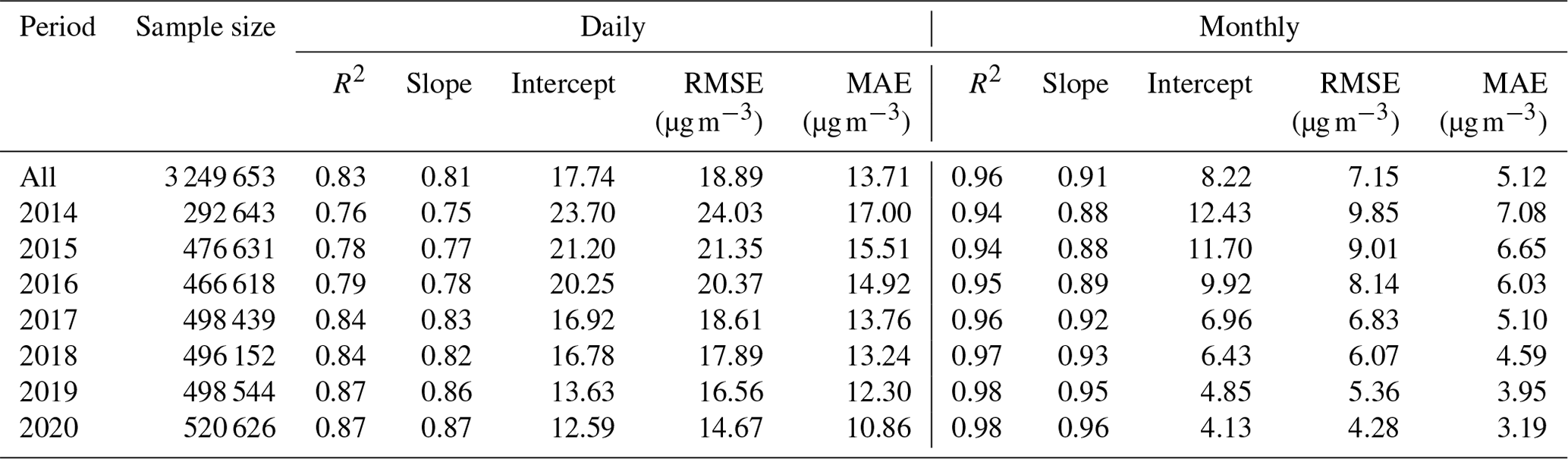
Table 1 presents the random 10-fold CV results of our proposed method, showing that our MDA8 estimates closely align with the measured MDA8 O₃ concentrations. For the CV over the entire modeling period, the R² values for daily and monthly MDA8 estimates were 0.83 and 0.96, respectively. The corresponding RMSE (MAE) values were 18.89 µg m⁻³ (13.71 µg m⁻³) for daily estimates and 7.15 µg m⁻³ (5.12 µg m⁻³) for monthly estimates. We further compiled the CV results by province, and the XGBoost model excelled in Beijing, Tianjin, Hebei, Shanxi, and Henan provinces/cities, achieving CV R² values above 0.86, but it performed less well in Fujian and Taiwan, where R² values were below 0.70 (Fig. S3). When examined by year, the R² (RMSE) values improved from 0.76 (24.03 µg m⁻³) in 2014 to 0.87 (14.67 µg m⁻³) in 2020. This improvement is primarily attributed to the increased sample size resulting from the addition of more monitoring stations in later years. Additionally, the estimation accuracy metrics at the monthly level were significantly better than those at the daily level, suggesting that temporal averaging can mitigate the uncertainty in model estimates. Overall, focusing on estimation accuracy, our proposed method achieves performance that is superior to, or at least comparable with, previous ozone modeling studies, with sample-based, 10-fold CV R² values at the daily level ranging from 0.70 to 0.87 (Table S4) (Ma et al., 2022a; Liu et al., 2020; Xue et al., 2020; Zhu et al., 2022; Chen et al., 2021; Wei et al., 2022).

Table 1 The random 10-fold CV results for the proposed long-term MDA8 O₃ modeling method.

3.1.2 Evaluation of pre-2013 estimates

We employed a rigorous validation approach, namely the leave-1-year-out CV, to assess the model's predictive capability for years lacking national ground-level O₃ monitoring data. Figure 1a illustrates that our proposed modeling framework predicts historical O₃ data with somewhat high estimation uncertainty at the daily level (i.e., R²=0.57, RMSE = 29.72 µg m⁻³, and MAE = 22.11 µg m⁻³) and reduced uncertainties at the monthly level (i.e., R²=0.74, RMSE  = 17.75  µg m⁻³, and MAE = 12.76 µg m⁻³). Additionally, an independent evaluation using 17 122 ozone measurements from Hong Kong, spanning 2005 to 2012, demonstrates that our model achieved R² values ranging from 0.31 to 0.59 and RMSE values from 34.65 to 45.40 µg m⁻³, with averages of 0.41 and 41.95 µg m⁻³, respectively (Fig. 1b and Table S5). These results are comparable to those from the leave-1-year-out CV conducted over Hong Kong (i.e., R²=0.44, RMSE  = 32.84 µg m⁻³, and MAE = 24.86 µg m⁻³ in Table S6). This consistency underscores the reliability of the leave-1-year-out CV for assessing the model's predictive performance for periods without national ground-level ozone measurements.

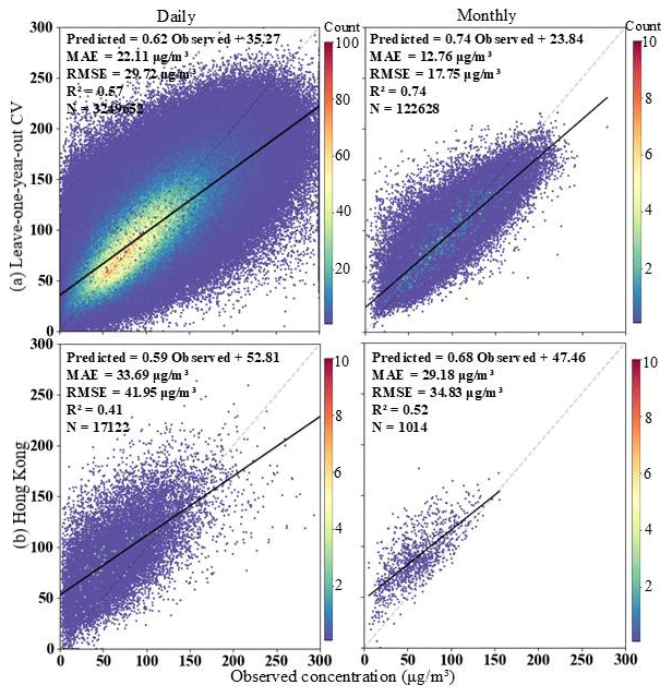
Figure 1 Validation results of historical MDA8 O₃ estimates. (a) Leave-1-year-out CV at daily and monthly levels. (b) Independent validation results against monitoring data from Hong Kong (2005–2012), where the monitoring data over Hong Kong were not employed in model development.

While several studies have developed long-term O₃ estimation models for China, few studies have quantitatively evaluated the predictive accuracy of their models' pre-2013 estimates (Table S4). Two studies (Liu et al., 2020; Ma et al., 2022a) reported that these models predicted pre-2013 MDA8 O₃ concentrations with leave-1-year-out CV R² (RMSE) of 0.69 (19.47 µg m⁻³) and day-based 10-fold CV R² of 0.63 at the monthly level, respectively. Compared with these earlier long-term ozone modeling studies (Table S4), our results demonstrate greater reliability for historical years without ground-level ozone measurements, with stronger leave-1-year-out CV and day-based 10-fold CV results, particularly at the aggregated monthly level (Chen et al., 2021; Liu et al., 2020; Ma et al., 2022a; Xue et al., 2020; Zhu et al., 2022; Wei et al., 2022). These findings indicate that our model not only captures long-term trends but also captures the fine-scale variations in ozone across China more accurately, making it valuable for both long-term and short-term ozone variation and exposure research.

3.1.3 Estimated high-resolution maps of ground-level ozone

We selected a subset from June 2018, identified as a hotspot for high ozone levels based on ground-level monitoring data, from our long-term, full-coverage MDA8 O₃ estimates generated by the proposed modeling framework. This subset was used to evaluate whether the extrapolated surfaces accurately capture day-to-day and fine-scale variations in ground-level ozone concentrations. Figure 2a–d present a comparison of monthly mean ground-level MDA8 O₃ concentrations from our high-resolution estimates with the 10 km MDA8 estimates by Wei et al., (2022) and in situ measurements for June 2018 – a month noted for high ozone concentrations at the monitoring stations. The nationwide distributions illustrate that our model successfully captures the general spatial variation pattern of ground-level ozone across China, aligning well with both the findings of Wei et al. (2022) and measured values (Fig. 2a). Zoomed-in maps of Jinan, Wuhan, and Chongqing highlight that our modeling approach predicts fine structures in ground-level ozone concentrations that are not discernible in coarser-resolution maps and in situ measurements (Fig. 2b–d). Additionally, comparisons of daily time series of MDA8 O₃ estimates versus observations in 2018 (Figs. 2d and S4) show that our method effectively captures daily and seasonal variability, although it tends to underestimate extremely high concentrations. This underestimation is likely due to the regression approach, which optimizes predictions based on average behavior. Overall, while 10 km and in situ data primarily identify broad “hotspots” of ground-level ozone (e.g., at the city scale), our high-resolution predictions uncover much more intricate structures, capturing sharp spatial and temporal gradients shaped by both natural and anthropogenic factors.

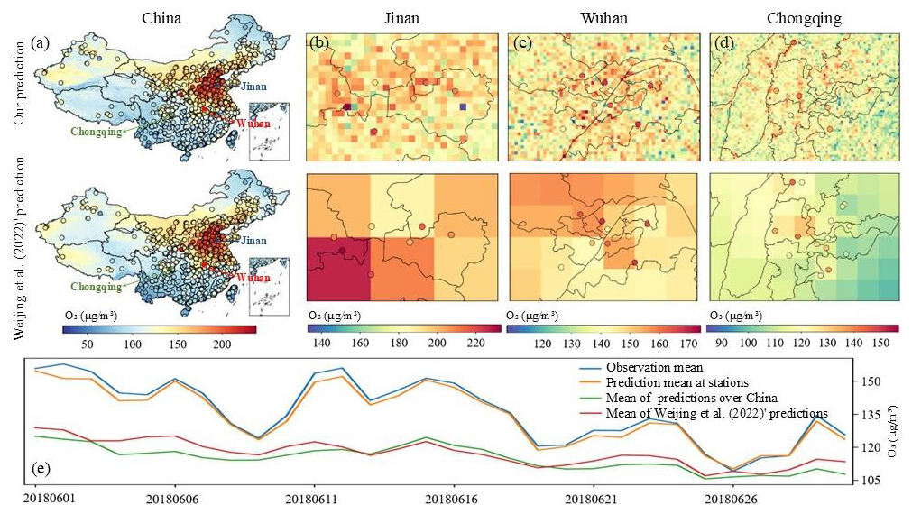
Figure 2 Spatiotemporal comparisons of ground-level ozone predictions vs. observations in China in June 2018. (a) Monthly mean map of MDA8 O₃ predictions with station ozone measurements (monthly valid measurements >15 for each station). Zoomed-in maps over (b) Jinan, (c) Wuhan, and (d) Chongqing. (e) Time series of mean MDA8 O₃ concentrations over China during June 2018 referenced as YYYYMMDD.

3.2 Spatial distribution and long-term trend of ground-level O₃ exposure

Figure 3a illustrates how long-term pollution hotspots vary by region and season. In spring, moderate O₃ pollution is widespread in the eastern region, with most MDA8 O₃ concentrations ranging between 100 and 120 µg m⁻³, except in the southern provinces. Summer sees severe ozone pollution, with concentrations exceeding 100 µg m⁻³ in most areas, apart from the Qinghai–Tibet plateau and Yunnan Province. During this season, the central North China Plain (NCP) experiences the highest pollution levels, with 21-year mean MDA8 O₃ concentrations routinely surpassing 140 µg m⁻³. In autumn, the southern provinces experience mild ozone pollution with most MDA8 O₃ levels between 100 and 110 µg m⁻³, while the Pearl River Delta (PRD) becomes the prominent ozone exposure hotspot, with most concentrations exceeding 120 µg m⁻³. Winter features the lowest ozone levels, with nearly all regions recording MDA8 O₃ concentrations below 100 µg m⁻³. Consequently, we identified eastern China, the NCP, and the PRD as long-term high-exposure ozone regions, which were given special attention in the subsequent analysis.

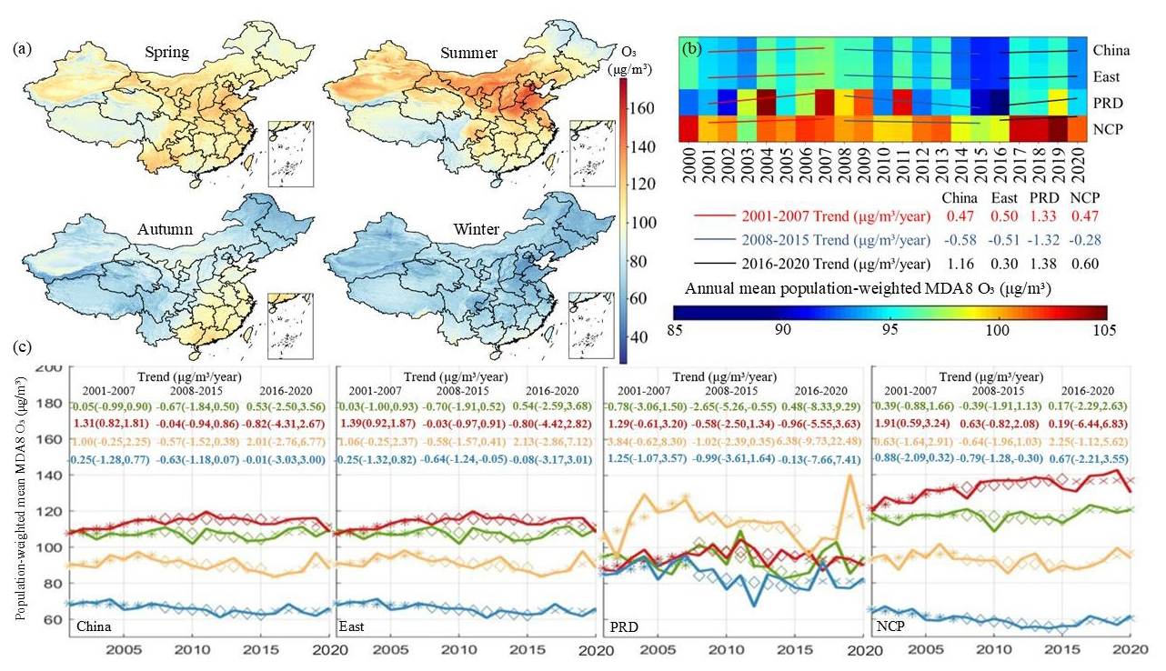
Figure 3 Overall spatiotemporal patterns of exposure to ground-level ozone in China over the past 2 decades. (a) Spatial map of seasonal mean MDA8 O₃ concentrations 2000–2020. (b) Annual mean population-weighted MDA8 O₃ concentrations over China and the three regions (i.e., eastern China, PRD, and NCP). (c) Seasonal population-weighted mean MDA8 O₃ concentrations over China and three typical regions, and their linear trends (green for spring, red for summer, orange for autumn, and blue for winter), where asterisks (*), diamonds (◊), and crosses (x) correspond to the linear trends in the 2001–2007, 2008–2015, and 2016–2020 sub-periods, respectively, with 95 % confidence intervals and colors matched to seasons.

By integrating yearly population distributions from LandScan (Rose et al., 2020), we analyzed the spatiotemporal patterns of exposure to ground-level ozone across China over the past 2 decades. Figure 3b–c show the annual and seasonal trends of population-weighted mean MDA8 O₃ concentrations, revealing long-term trends that are non-monotonic and vary significantly across different regions. As illustrated in the annual exposure time series (Fig. 3b), two turning points are observed around 2008 and 2015: in the first phase of 2001–2007, the population-weighted exposure to ozone increased with a linear slope of 0.47 $\mathrm{\mu }\mathrm{g}{\mathrm{m}}^{-\mathrm{3}}{\mathrm{yr}}^{-\mathrm{1}}$, then decreased post-2008 with a slope of −0.58 $\mathrm{\mu }\mathrm{g}{\mathrm{m}}^{-\mathrm{3}}{\mathrm{yr}}^{-\mathrm{1}}$, followed by a substantial rise at a rate of 1.16 $\mathrm{\mu }\mathrm{g}{\mathrm{m}}^{-\mathrm{3}}{\mathrm{yr}}^{-\mathrm{1}}$ during the third phase of 2016–2020. These shifting exposure trajectories also displayed pronounced seasonal and regional variations (Fig. 3c). During the 2001–2007 phase, eastern China and the NCP experienced a significant rise in ozone exposure during the summer months, with slopes ranging from 1.39 to 1.91 $\mathrm{\mu }\mathrm{g}{\mathrm{m}}^{-\mathrm{3}}{\mathrm{yr}}^{-\mathrm{1}}$, whereas the PRD region saw its most substantial increases in autumn, with a notable slope of 3.84 $\mathrm{\mu }\mathrm{g}{\mathrm{m}}^{-\mathrm{3}}{\mathrm{yr}}^{-\mathrm{1}}$. In the second phase, the three typical ozone hotspots generally showed decreasing trends across all seasons (slopes from −0.03 to −1.02 $\mathrm{\mu }\mathrm{g}{\mathrm{m}}^{-\mathrm{3}}{\mathrm{yr}}^{-\mathrm{1}}$), except for a slight increase during the summer in the NCP (slope of 0.64 $\mathrm{\mu }\mathrm{g}{\mathrm{m}}^{-\mathrm{3}}{\mathrm{yr}}^{-\mathrm{1}}$). Moving into the 2016–2020 phase, these typical hotspots transitioned to marked increasing trends in autumn, particularly in the PRD, which displayed a steep increase with a slope of 6.38 $\mathrm{\mu }\mathrm{g}{\mathrm{m}}^{-\mathrm{3}}{\mathrm{yr}}^{-\mathrm{1}}$. Conversely, while other regions exhibited declining trends during the summer season of this phase, the NCP continued to show an upward trend with a slope of 0.19 $\mathrm{\mu }\mathrm{g}{\mathrm{m}}^{-\mathrm{3}}{\mathrm{yr}}^{-\mathrm{1}}$.

3.3 Monthly exposure and county-level pattern

To investigate how the most severe ozone pollution events and baseline levels have evolved over time, we further analyzed monthly exposure patterns, focusing specifically on the trends in monthly population-weighted mean MDA8 ozone concentration peaks and troughs across China and three key regions. Overall, the monthly ozone concentrations followed a three-phase trend, similar to the annual patterns identified earlier (as shown in Figs. S5 and 3b), with slight regional variations in the slopes. However, a closer examination of the monthly peaks and troughs revealed distinct changes. As indicated in Fig. 4a, all regions experienced an increase during the first phase, with the PRD recording a notable rise at a rate of 4.37 $\mathrm{\mu }\mathrm{g}{\mathrm{m}}^{-\mathrm{3}}{\mathrm{yr}}^{-\mathrm{1}}$. The second phase showed general declines across most regions (slopes range from −0.99 to −1.19 $\mathrm{\mu }\mathrm{g}{\mathrm{m}}^{-\mathrm{3}}{\mathrm{yr}}^{-\mathrm{1}}$), except for the PRD (slope = −0.009 $\mathrm{\mu }\mathrm{g}{\mathrm{m}}^{-\mathrm{3}}{\mathrm{yr}}^{-\mathrm{1}}$), which remained relatively stable. The subsequent phase again saw slope increases in all regions, ranging from 0.19 to 0.44 $\mathrm{\mu }\mathrm{g}{\mathrm{m}}^{-\mathrm{3}}{\mathrm{yr}}^{-\mathrm{1}}$, with the PRD experiencing a significant uptick at a slope of 3.19 $\mathrm{\mu }\mathrm{g}{\mathrm{m}}^{-\mathrm{3}}{\mathrm{yr}}^{-\mathrm{1}}$. The trends in monthly troughs mirrored the decline observed in the second phase, albeit with varied patterns in other stages. From 2001 to 2007, both China and eastern China registered slight increases, whereas the NCP and PRD noted decreases in trough levels. During the 2016–2020 period, the PRD showed a marked increase, with a slope of 2.81 $\mathrm{\mu }\mathrm{g}{\mathrm{m}}^{-\mathrm{3}}{\mathrm{yr}}^{-\mathrm{1}}$, contrasting with decreases ranging from −0.33 to −0.52 $\mathrm{\mu }\mathrm{g}{\mathrm{m}}^{-\mathrm{3}}{\mathrm{yr}}^{-\mathrm{1}}$ in the other regions. Additionally, over the past 2 decades, the monthly peaks predominantly occurred in June. However, results from the Mann–Kendall test (Table S7) indicate a significant shift in the timing of peak ozone concentrations across most of China, with p values below 0.05 for China, eastern China, and the NCP, suggesting a potential shift from June to earlier in May in recent years.

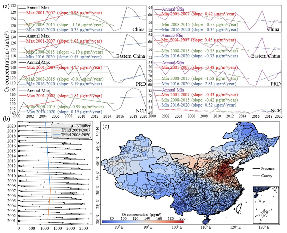
Figure 4 Spatiotemporal distributions of monthly population-weighted mean MDA8 O₃ concentrations over China and the three typical regions. (a) Time series with three-piece trend lines of peaks (left panel) and troughs (right panel) from 2001 to 2020. (b) Number of counties with monthly ozone concentrations exceeding 100 µg m⁻³ from 2000 to 2020. (c) Spatial distribution of county-level mean concentrations in June 2018.

To provide a spatial and temporal overview of severe ozone pollution trends across counties in China, we tracked the number of counties where monthly ozone concentrations exceeded 100 µg m⁻³ from 2000 to 2020. As shown in Fig. 4b, the trend exhibits significant seasonal variation each year, with peaks typically occurring in late spring and early autumn. While the seasonal pattern remained consistent annually, the amplitude of these peaks fluctuated from year to year. Notably, in May 2017, 2812 counties exceeded the ozone threshold, compared to an average of 2543 counties during the month of May in other years. On average, 1142 of the 2900 counties exceeded this 100 µg m⁻³ threshold on a monthly basis, with the 25th and 75th percentiles at 38 and 2002 counties, respectively. Interestingly, the time series for the number of counties with exceedances did not parallel the three-phase variation identified earlier. Instead, the number of counties exceeding the threshold increased from 2001 to ∼2007, with a slope of 16.84 yr⁻¹, and then decreased in the subsequent years, with a slope of -12.44 yr⁻¹.

Figure 4c displays a county-level spatial map from June 2018, a month identified as a hotspot for high ozone levels, highlighting significant spatial disparities in ozone exposure within cities. For example, in Beijing, the population-weighted mean MDA8 O₃ concentrations ranged from 141.23 µg m⁻³ in Yanqing in the northwest to 180.33 µg m⁻³ in Tongzhou in the southeast. Nationally, the highest exposure levels were recorded in Xiqing and Beichen counties in Tianjin, with concentrations around 200 µg m⁻³. Conversely, the lowest exposures were observed in two southwestern counties in Yunnan Province and three southeastern counties in Hainan Province, with concentrations below 70 µg m⁻³.

3.4 Short-term exposure characteristics and extreme episodes of ground-level O₃

We observed the day-to-day variation in ground-level ozone concentrations for China as a whole and for the three typical regions over the past 2 decades. The coefficient of variation of the daily MDA8 O₃ predictions indicates significant spatial heterogeneity in the nationwide distribution of ambient ozone, with values ranging from 0.16 to 0.41 (Fig. S6). This variability is characterized by notable seasonality, displaying the highest mean value in autumn (0.29) and the lowest in spring (0.22).

Overlaying daily MDA8 O₃ predictions with population distribution, Fig. 5a reveals that from March 2000 to December 2020, over 60 % of the Chinese population was exposed to MDA8 O₃ concentrations exceeding 100 µg m⁻³ – a concentration defined as the first level of the national ambient air quality standard – on more than 31 % of the total prediction days. The long-term variation in these exposure ratios follows a three-phase pattern (Fig. S7) similar to the annual ozone exposure trend identified in Sect. 3.2. The highest exposure months are May and June, with daily proportions around 70 %. Particularly in May 2007 and 2017, the average proportion reached 79 %, ranging between 56 % and 97 %. At the regional level, daily ozone exposure in the three typical ozone exposure hotspots was more severe than the national average, especially for the NCP and PRD regions. In these regions, ∼60 % and ∼40 % of days, respectively, saw the population exposed to ozone levels above 100 µg m⁻³. Furthermore, ∼5 % of days in the NCP and ∼2 % in the PRD exceeded the national second-level limit of 160 µg m⁻³ (Fig. 5b). The spatial map in Fig. 5c further illustrates that extremely severe ozone exposure was concentrated in the NCP region, especially for the central NCP, where most areas experienced more than 10 % of days with concentrations exceeding 160 µg m⁻³. Over time, this severe exposure expanded from part of south Hebei, Tianjin, north Henan, and west Shandong in the first phase (2001–2007) to cover most of the NCP region by the third phase (2016–2020).

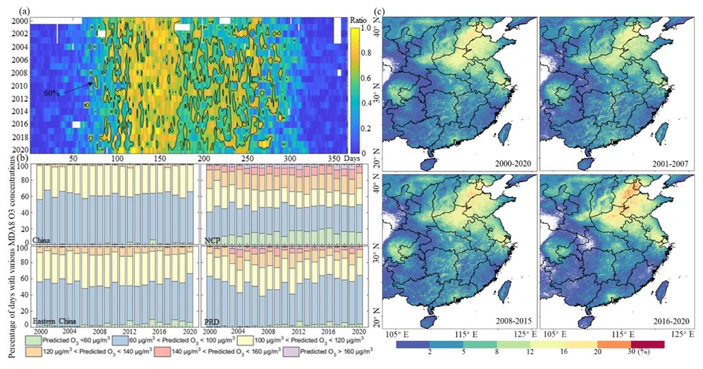
Figure 5 Day-to-day patterns of ground-level ozone exposure levels from 2000 to 2020. (a) Heatmap of daily ratios of the population exposed to MDA8 O₃ concentration exceeding 100 µg m⁻³. (b) Percentage of days with various MDA8 O₃ concentrations. (c) High-exposure risk maps calculated for 2000–2020 and the three phases.

Severe ozone pollution events are usually associated with meteorological conditions (Yang et al., 2024). Figure 6 exemplifies an extreme ozone pollution episode that occurred from 25 June to 5 July 2017 over the NCP. The West Pacific Subtropical High, positioned between 20 and 26° N, significantly influenced ozone distribution over the Yangtze River Delta by modulating precipitation and solar radiation. High relative humidity in the region suppressed ozone formation, resulting in lower concentrations. In contrast, the Beijing–Tianjin–Hebei (BTH) region and its surrounding areas experienced favorable conditions for ozone production due to an anomalous high-pressure system in the upper troposphere (Xu et al., 2019). Warm, southerly winds in the lower troposphere contributed to higher temperatures and the northward transport of aged air masses, increasing ozone and its precursors. Furthermore, a persistent temperature inversion in the BTH trapped pollutants in lower layers of the atmosphere, exacerbating ozone pollution. This inversion preserved ozone at night and facilitated its descent to the surface at sunrise, worsening the pollution. These persistent conditions sustained severe regional ozone pollution events in the BTH (Mao et al., 2020).

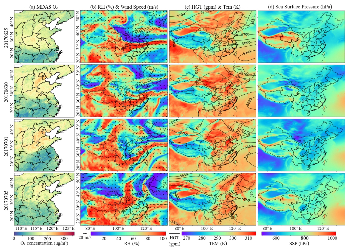
Figure 6 Spatial distributions of daily MDA8 O₃ (a)  and meteorological fields (b) relative humidity (RH) and wind speed (WS) at 500 hPa, (c) geopotential height field (HGT) at 500 hPa and air temperature (T) at 2 m, and (d) sea surface pressure (SSP) for 25 June–5 July 2017 referenced as YYYYMMDD.

4 Discussion

In this study, we developed an XGBoost-based prediction model to hindcast long-term, full-coverage, ground-level MDA8 O₃ concentrations across China, with daily and 1 km spatiotemporal resolution. To the best of our knowledge, our model's performance, with a sample-based 10-fold CV R² of 0.83 at the daily level, is comparable to other national-scale ozone modeling studies in China, which have reported validation R² values ranging from 0.77 to 0.87 (Table S4). Despite similar performance levels, our modeling framework offers superior spatiotemporal resolution (daily and 1 km vs. monthly or 0.05° or coarser) and covers a longer prediction period (2000–2020 vs. 2005–2019 or shorter) compared to previously mentioned studies. The rigorous hindcast and individual validation results confirm that our long-term estimates reasonably represent day-to-day trends and intraurban variations in ground-level ozone, including for the pre-2013 period. The long-term, full-coverage estimates capture short-term local pollution variations and details not revealed by previously coarser-resolution or shorter-period data (Figs. 1 and 3). For example, Fig. S8 illustrates a case study from Wuhan on 28 May 2017, a day characterized by elevated ozone levels, showing local NO₂ levels titrated O₃, resulting in observed ozone concentrations that are lower than those downwind. Consistent with our previous findings (He et al., 2024), incorporating LST – closely linked to ozone variations and available at high spatiotemporal resolutions – significantly enhances the overall quality of our estimation data. This improvement is demonstrated by its leading rank in variable importance (Fig. S9) and the observed increase in R² values by 0.04–0.06 across sample-, site-, and day-based 10-fold CVs when comparing models with and without LST (Table S8). Additionally, its critical role in hindcasting ground-level ozone estimates for the pre-2013 unmonitored period is validated through improvements in estimation accuracy, as reflected by an R² increase of 0.07 in the leave-1-year-out CV (Table S8) and 0.02 in independent validation using Hong Kong in situ measurements (Table S9). Additionally, the inclusion of other spatiotemporal covariates related to ozone formation and dispersion, such as radiation, terrain, and the ozone precursor NO₂, helps the model capture the complex spatiotemporal dynamics of ground-level ozone.

Our long-term trend analysis reveals a three-phase variation pattern in ground-level ozone across China over the past 2 decades, characterized by significant seasonality and regional disparities (Figs. 3, S5, 4). This pattern likely results from a complex interplay of environmental, regulatory, and climatic factors influencing ozone levels. Similar to long-term PM_2.5 trends in China (He et al., 2023), the first 2001–2007 phase presented an increasing trend, possibly linked to rapid industrial growth and urbanization, accompanied by lenient environmental controls. This period likely saw higher emissions of ozone precursors such as volatile organic compounds (VOCs) and nitrogen oxides (NO_x) (Akimoto, 2003; Ahammed et al., 2006). In contrast, the second phase featured a general decline in ozone levels, coinciding with stricter air quality policies implemented by the central government, which included notable reductions in nitrate emissions observed during 2012–2016 (Wang et al., 2019). However, unlike PM_2.5 trends, which experienced a marked decrease after 2013, ground-level ozone entered a third phase (2016–2020) of substantial increase. This divergence can be partly attributed to the decline in PM_2.5 levels, which likely slowed the removal of hydroperoxy radicals, thereby enhancing ozone production (Li et al., 2019). These findings highlight the critical need for integrated control of ozone and PM_2.5 pollution to avoid unintended trade-offs between these pollutants.

Our ozone exposure analysis identified several hotspots, with the most severe exposures – concentrations exceeding 160 µg m⁻³ – primarily observed in the NCP. This region has experienced an increasing trend in both the geographical extent and frequency of these high concentrations (Fig. 5). Temporally, we observed a notable shift in the peak ozone exposure month from June to May, especially pronounced in the NCP. This escalation in ozone pollution levels and the earlier annual peak may be attributed to changes in meteorological conditions, such as extremely high temperatures (Wang et al., 2022a), and air pollutant emissions – notably the reduction in NO_x emissions coupled with high emissions of VOCs (Ke et al., 2021) – which are conducive to ozone formation. Furthermore, the significant reduction in ambient particulate matter in the NCP in recent years has also contributed to worsening ozone conditions in this region (Li and Li, 2023). These shifts in spatial and temporal exposure hotspots should raise significant concern for both central and local governments, as the expanding extent and prolonged duration of high ozone levels could exacerbate public health risks and broadly impact agricultural productivity. Furthermore, the distribution of ozone exposure hotspots presents significant seasonal changes, with summertime hotspots predominantly occurring in the NCP and shifting to the PRD during autumn (Fig. 3). These differing trends highlight the critical role of regional weather patterns in shaping ozone dynamics. As a result, policy measures should be carefully tailored to address not only the unique needs of specific regions but also the seasons during which ozone peaks are most pronounced, ensuring more effective and targeted mitigation strategies.

Based on high-resolution estimates, we quantitatively identified counties with the highest and lowest ozone levels (Fig. 4b–c), offering critical insights to inform resource allocation and targeted pollution control measures. For instance, counties such as Xiqing and Beichen in Tianjin, identified as having high ozone levels, can be prioritized for implementing targeted emission control policies and public health campaigns to mitigate health risks for local residents. These localized insights are often overlooked in broader-scale regional analyses. Previous studies relying on coarser-resolution data have typically focused on large urban agglomerations, such as the Beijing–Tianjin–Hebei region and the Pearl River Delta (PRD) (Wei et al., 2022), neglecting smaller yet critically affected areas. Conversely, while pixel-level analyses offer highly detailed spatial patterns, they may lack the administrative relevance needed for actionable policy decisions. By bridging the gap between regional and pixel-level analyses, our county-level analysis provides actionable and geographically specific recommendations, empowering policymakers to address ozone pollution more effectively.

The primary source of uncertainty in this study lies in the long-term ozone estimates. Since the NAQMN was not established before 2013, monitoring data from earlier years are unavailable. As a result, we could not directly train the model for that period. Instead, we applied the model developed for post-2014 data to hindcast ozone levels for the earlier unmonitored years. Consequently, the estimated ozone levels for these years may carry a certain degree of uncertainty, which could impact the spatiotemporal analysis. However, we conducted rigorous validation of the hindcast estimates, and the time-aggregated validation results demonstrated significant improvements in the accuracy of the pre-2013 estimates (R²=0.74 at the monthly scale in Fig. 1). These findings suggest that the spatiotemporal exposure analysis, particularly regarding long-term variations, is robust and reliable.

5 Conclusions

In this study, we developed a multi-source, high-resolution modeling method using the XGBoost algorithm to hindcast long-term ground-level ozone concentrations across China. By utilizing this approach, we generated daily ozone estimates from 2000 to 2020, enabling the analysis of spatiotemporal exposure characteristics across multiple scales. The key findings of this study are summarized as follows:

1. Improved ozone hindcasting using satellite LST. We successfully extended our high-resolution ozone modeling method by incorporating satellite-derived LST as a primary predictor. This enhancement improved the accuracy of hindcasting ozone concentrations over historically unmonitored periods. Comparative results confirmed that the inclusion of satellite LST significantly strengthened the model's long-term performance.

2. Non-monotonic long-term trends and seasonal shifts. Our long-term analysis revealed a three-phase variation pattern in ground-level ozone levels over the past 2 decades, marked by regional and seasonal fluctuations. From 2001 to 2007, ozone concentrations increased at a rate of 0.47 $\mathrm{\mu }\mathrm{g}{\mathrm{m}}^{-\mathrm{3}}{\mathrm{yr}}^{-\mathrm{1}}$, followed by a decline post-2008 at a rate of −0.58 $\mathrm{\mu }\mathrm{g}{\mathrm{m}}^{-\mathrm{3}}{\mathrm{yr}}^{-\mathrm{1}}$ and a significant rise during 2016–2020 at a rate of 1.16 $\mathrm{\mu }\mathrm{g}{\mathrm{m}}^{-\mathrm{3}}{\mathrm{yr}}^{-\mathrm{1}}$. Seasonal shifts were prominent, with high ozone levels concentrated in spring in eastern China, summer in the NCP, and autumn in the PRD. Notably, the PRD exhibited a sharp increase in autumn ozone levels during the third phase, with a rate of 6.38 $\mathrm{\mu }\mathrm{g}{\mathrm{m}}^{-\mathrm{3}}{\mathrm{yr}}^{-\mathrm{1}}$.

3. Emerging exposure hotspots. Our exposure analysis identified ozone concentrations exceeding 100 µg m⁻³, which historically peaked in June but have shifted to peak earlier, in May, in recent years. Additionally, dangerous exposure levels above 160 µg m⁻³ were predominantly concentrated in the NCP, with trends of expansion in terms of extent and duration. Day-to-day analyses of ozone pollution episodes further underscored the role of meteorological conditions in driving extreme ozone events.

Overall, our rigorously validated estimates and exposure analyses provide critical data to inform environmental policymaking and public health research, laying the groundwork for targeted interventions to mitigate ozone exposure risks.