Stratospheric Aerosol Intervention experiment for the Chemistry–Climate Model Initiative

A new Stratospheric Aerosol Intervention (SAI) experiment has been designed for the Chemistry–Climate Model Initiative (CCMI-2022) to assess the impacts of SAI on stratospheric chemistry and dynamical responses and inter-model differences using a constrained setup with a prescribed stratospheric aerosol distribution and fixed sea surface temperatures and sea ice. This paper serves a dual purpose: first, it describes the details of the experimental setup and the prescribed aerosol distribution and demonstrates the suitability of the simplified setup to study SAI impacts in the stratosphere in a multi-model framework. The experiment allows attributing inter-model differences to the resulting impacts on atmospheric chemistry, radiation, and dynamics rather than the model uncertainty arising from differences in aerosol forcing and feedbacks from the ocean and sea ice under SAI. Second, we use the Whole Atmosphere Community Climate Model (WACCM6) to compare the interactive stratospheric aerosol configuration with coupling to land, ocean, and sea ice used to produce the stratospheric aerosol distribution with the results of the constrained SAI experiment. With this, we identify and isolate the stratosphere-controlled SAI-induced impacts from those influenced by the coupling with the ocean. Overall, this comparison facilitates an advanced process-level understanding of the drivers of SAI-induced atmospheric responses. For example, we confirm earlier suggestions that the SAI-induced positive phase of the North Atlantic Oscillation in winter, with the corresponding winter warming over Eurasia and related changes, is driven by stratosphere–troposphere coupling. Future multi-model comparisons will thus provide an important contribution to upcoming scientific assessments of ozone depletion.

1 Introduction

Recent studies have identified significant impacts of sulfur-based Stratospheric Aerosol Intervention (SAI) on the stratosphere and below due to its effects on atmospheric chemistry, dynamics, and radiation (e.g., WMO, 2022). However, model-specific differences resulted in a significant inter-model spread in the simulated SAI responses, including differences in aerosol loading, distribution, and the resulting climate feedbacks (Pitari et al., 2014; Tilmes et al., 2022). Furthermore, only very few Earth system models (ESMs) that are interactively coupled with the ocean and cryosphere can interactively simulate stratospheric aerosols, chemistry, and dynamics in the atmosphere, as is required for the recent Geoengineering Model Intercomparison Project (GeoMIP) experiments (Visioni et al., 2023).

A multi-model intercomparison study by Tilmes et al. (2022)​​​​​​​, which investigated the impacts of SAI on the stratospheric composition and ozone, was based on the GeoMIP G6sulfur and G6solar experiments (Visioni et al., 2021b). This experiment used the CMIP6 SSP5-8.5 high-end greenhouse gas (GHG) forcing scenario (Gidden et al., 2019; Meinshausen et al., 2020) as a baseline. It required sulfur injections into the tropical lower stratosphere (10° N–10° S) to produce global mean surface temperatures close to those simulated for the middle-of-the-road SSP2-4.5 GHG scenario. Only six ESMs performed the G6sulfur simulations, either prescribing aerosol properties scaled from earlier model experiments or deriving the aerosol distribution interactively from SO₂ gas injections (Visioni et al., 2021b). Of these six models, only three included interactive stratospheric chemistry, and only two included comprehensive aerosol microphysical processes. The resulting aerosol distributions and surface area density (SAD) strongly differed in structure, location, and magnitude. Consequently, these differences led to different chemical processing and radiative heating responses that impact transport and ozone (Tilmes et al., 2022). Furthermore, besides the relative large-scale cooling from SAI, simulated regional changes in surface climate are a result of the influence of stratospheric changes or induced by the residual feedbacks from the ocean or land surface (Banerjee et al., 2021; Wunderlin et al., 2024; Bednarz et al., 2023). Due to the range of factors contributing to the simulated SAI responses, it has been challenging to determine the reasons for inter-model differences.

To address these challenges, we have designed a new simplified SAI experiment that removes some of the complexity of previous experiments and constrains the models to impose the same SAI aerosol distribution and an internal model ocean surface temperature and sea ice climatology. With this, we exclude two sources of uncertainty contributing to significant differences in multi-model comparison studies. In particular, such experimental design removes the uncertainty in the model representation of aerosol microphysical processes and, hence, isolates inter-model differences in the stratospheric chemistry and circulation response to SAI under the same aerosol perturbation. In addition, the prescribed ocean and sea ice conditions remove the influence of model-to-model differences in climate sensitivity that would require different injection amounts in an interactive setting. Furthermore, by removing these feedbacks, this experimental setup also allows us to isolate the stratospheric (top-down) impact of SAI on the troposphere and removes any potential (bottom-up) influences from an uncertain ocean response. Finally, the model setup allows more modeling groups that do not include comprehensive aerosol microphysics or ocean coupling to participate in SAI experiments.

In the first part of this paper, we describe the technical details of the SAI experiments and detail the procedure behind producing the aerosol properties to be prescribed by models. The proposed CCMI experiment has been designed for models participating in the second phase of the Chemistry–Climate Model Initiative (CCMI-2022). CCMI is a follow-up project on the Chemistry–Climate Model Validation (CCMVal and CCMVal-2) activity. The CCMVal simulations were used for multi-model assessment of a range of stratosphere-related processes, most importantly in support of the earlier Ozone Assessment Reports (WMO, 2007, 2010), as well as used to produce a comprehensive assessment report on chemistry–climate model evaluation and performance (Eyring et al., 2010). The latest set of CCMI-2022 experiments was defined by Plummer et al. (2021). State-of-the-art chemistry–climate models with interactive chemistry that participated in CMIP6 performed reasonably well regarding the historical and future evolution of stratospheric species, including ozone (e.g., Keeble et al., 2021). In CCMI-2022, only three of eight models included an interactive ocean to perform future experiments. The models without that capability can prescribe sea surface temperatures (SSTs) and sea ice from other models (Plummer et al., 2021).

The second part of the paper compares the results of two SAI simulations that differ mainly in the model setup, (i) a fully coupled SAI simulation with interactive aerosols and ocean and (ii) an analogous senD2-sai experiment with prescribed stratospheric aerosols and fixed SSTs and sea ice. This allows us to assess the validity of the senD2-sai experiment with regard to SAI-induced chemical and dynamical changes. It further helps to identify and isolate the stratosphere-controlled SAI-induced impacts from those influenced by the ocean and sea ice feedbacks. Various studies in the literature attempted to elucidate whether and how much SAI-induced stratospheric heating contributes to regional climate changes (Simpson et al., 2019; Banerjee et al., 2021; Jones et al., 2022; Bednarz et al., 2023). Other studies have also noted changes in the equatorial Pacific associated with the modulation of El Niño–Southern Oscillation variability under SAI (e.g., Zhang et al., 2024b) and identified changes in its teleconnections (e.g., Bednarz et al., 2023). With the experimental setup, for the first time, we can compare the results in interactive model simulation with the constrained setup in one modeling framework, allowing us to identify and isolate the importance of top-down stratospheric changes for the tropospheric climate response from the bottom-up feedbacks from changes in the ocean and sea ice.

The outline of the paper is as follows: we first introduce the model, as well as the different experiments that are used in this study in Sect. 2, including the setup and details of the CCMI SAI experiments designed for multi-model comparisons. In Sect. 3, we discuss differences between the constrained and interactive setup, including chemistry and dynamics, as well as differences in the response to surface climate. We conclude in Sect. 4.

2 Model description and experimental design

2.1 Model description

We use the Whole Atmosphere Community Climate Model version 6 (WACCM6), a configuration of the Community Earth System Model version 2 (CESM2) (Danabasoglu et al., 2020), to perform the experiments described below and summarized in Table 1. The atmospheric model includes comprehensive chemistry in the troposphere, stratosphere, mesosphere, and lower thermosphere (TSMLT) (Gettelman et al., 2019; Emmons et al., 2020). CESM2 (WACCM6), called WACCM6 in the following, uses a horizontal resolution of 0.9° × 1.25° and 70 levels in the vertical with a top at around 150 km. It includes a prognostic representation of tropospheric and stratospheric aerosols using Modal Aerosol Microphysics version 4 (MAM4) (Liu et al., 2016) and sulfur emissions from volcanoes and other sources (Mills et al., 2017). The model is coupled to the Community Land Model version 5 (CLM5) (Lawrence et al., 2019) and the Parallel Ocean Program version 2 (POP2) (Danabasoglu et al., 2020). Different model configurations allow it to be run with a prescribed stratospheric aerosol distribution and sea surface temperatures (SSTs) and sea ice, as required for the senD2-sai experiment.

Table 1 Overview of modeling experiments.

2.2 Experimental design

This section includes a description of the three types of model experiments used in this paper (as also outlined in Table 1). First, we discuss the fully interactive experiments coupled with ocean and sea ice, which provide information on future conditions without SAI, SSP2-4.5, and the equivalent CCMI experiment called senD2, defined by Plummer et al. (2021). Both experiments use the SSP2-4.5 future GHG scenario, although there are some minor differences for senD2. These simulations serve as a baseline setup for the CCMI SAI experiment.

Second, we describe the interactive SAI experiment, called SSP2-4.5 SAI. This experiment uses the same GHG scenario as SSP2-4.5 and, in addition, applies sulfur injections starting in the year 2025. This experiment calculates the stratospheric aerosol distribution used for the CCMI SAI experiments. Details about this setup are described in Sect. 2.2.2.

Third, we describe the CCMI SAI experiments (called senD2-sai and senD2-fix, defined by Plummer et al., 2021) to be adopted by other modeling groups in Sect. 2.2.3. The experiment senD2-sai uses the interactive senD2 setup as its baseline and prescribes stratospheric aerosols from the SSP2-4.5 SAI experiment, with elevated stratospheric aerosol starting in year 2025. In contrast to senD2, it uses an internal model climatology of fixed SSTs and sea ice between 2020 and 2030. To assess the effects of future changes with or without SAI, analyses are performed using comparisons between a future climate and a control climate for 2020–2030 conditions with background aerosol conditions. We introduce the experiment senD2-fix, with the same setup as senD2-sai, but using a stratospheric background aerosol distribution for the entire period to serve as a control for senD2-sai between 2020 and 2030.

2.2.1 Climate change simulations (SSP2-4.5 and refD2)

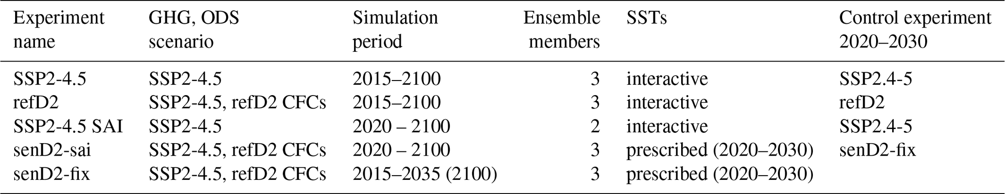
SSP2-4.5 is the middle-of-the-road CMIP6 scenario (Gidden et al., 2019; Meinshausen et al., 2020), and the CESM2 simulations were started in 2015 from the historical free-running simulations (Gettelman et al., 2019). The continuous increase in GHG concentration in SSP2-4.5 results in an increase in near-surface air temperature of around 2 °C and precipitation of 0.12 mm d⁻¹ by the end of the 21st century, compared to 2020–2030 conditions (Fig. 1a and b, green lines). For producing elevated stratospheric background aerosol conditions to represent eruptive volcanoes, the experiment used an average of the eruptive volcanic SO₂ emissions from 1850 to 2015, following the recommended CMIP6 setup for preindustrial control and future conditions (Danabasoglu et al., 2020). The simulated stratospheric aerosol optical depth (SAOD) at 525 nm wavelength in the model agrees well with observations from the Global Space-based Stratospheric Aerosol Climatology (GloSSAC) for stratosphere aerosol properties (Thomason et al., 2018) and remains higher than volcanically clean observed periods (Fig. 1c).

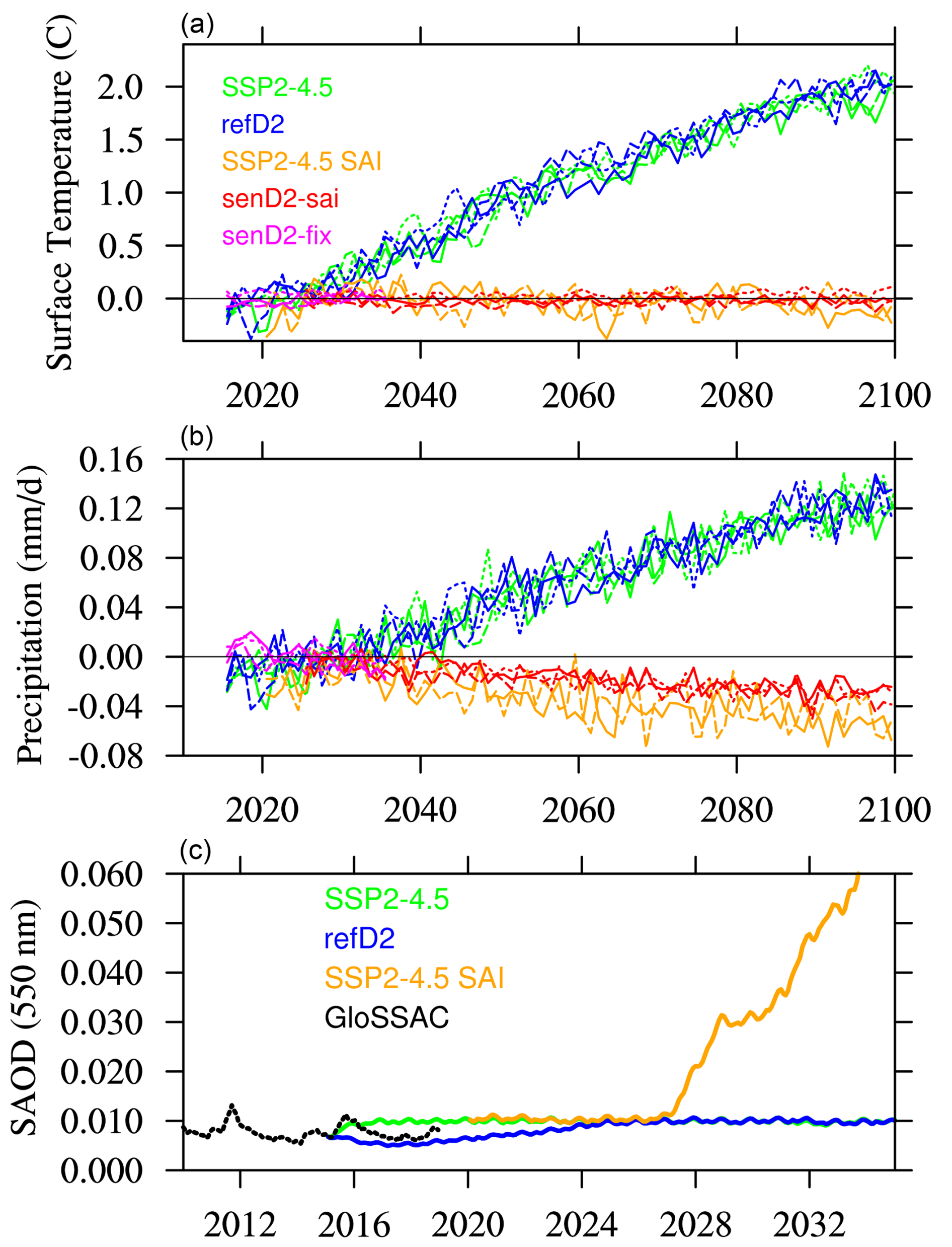
Figure 1 Changes in global mean air surface temperatures (a) and precipitation (b) compared to 2020–2030 average conditions, for available ensemble members (different line styles) for the different experiments performed with CESM2(WACCM6) (different colors). (c) Stratospheric aerosol optical depth averaged between 80° N and 80° S for GloSSAC observations (black) and the ensemble mean for different experiments performed with CESM2(WACCM6) (colored lines).

In WACCM6, the eruptive stratospheric volcano emissions between 2015 and 2025 were implemented slightly differently in SSP2-4.5 than in refD2, resulting in different stratospheric AOD (Fig. 1c). In refD2, eruptive sulfur injections transitioned from the current state in 2015 towards elevated background emissions described above within the first 10 years (Plummer et al., 2021), while in SSP2-4.5 these elevated emissions were implemented abruptly in 2015. The resulting lower SAOD in refD2 between 2015 and 2025 than the SSP2-4.5 experiment (Fig. 1c) is expected to result in differences in the climate response between SSP2-4.5 and refD2 in the first 10 years of the experiment using WACCM6. However, global near-surface temperature and precipitation differences are insignificant between the experiments, given the variability of global surface temperature and total precipitation (Fig. 1a and b, blue and green lines).

The CCMI-2022 future refD2 scenario uses GHG and aerosol forcings similar to the SSP2-4.5 experiment. However, the experiment uses the baseline scenario from WMO (2018) for halogenated ozone-depleting substances (ODS) that include small changes to the assumed future surface concentrations of ODS compared to those used in SSP2-4.5 (Plummer et al., 2021), leading to approximately 10 % higher future (2080–2099) stratospheric halogen (Cly and Bry) levels in refD2 compared to SSP2-4.5 (Fig. A1). The larger halogen levels in refD2 are expected to lead to differences when comparing the stratospheric ozone between refD2 and SSP2-4.5.

2.2.2 Interactive SAI simulation (SSP2-4.5 SAI)

The SSP2-4.5 SAI experiment produces the aerosol distribution input for senD2-sai and is based on the SSP2-4.5 setup using WACCM6, described above. When this experiment was performed, the refD2 experiment was unavailable, which would have been a more consistent control experiment than SSP2-4.5. However, despite small differences in future forcings, this experiment is expected to produce a similar stratospheric aerosol distribution. The experiment starts in 2020 from the corresponding SSP2-4.5 simulation, including CMIP6 GHGs and ODS, and elevated eruptive volcanic emissions described above. The injections of SO₂ start in 2025, 5 years after the start of the experiment to keep near-surface temperatures at 2020–2030 (inclusive) average conditions of the corresponding SSP2-4.5 simulation.

To achieve these temperature targets, we are using a similar setup as in previous SAI studies using WACCM6 (e.g., Tilmes et al., 2018a, 2022; Richter et al., 2022; Bednarz et al., 2023; Zhang et al., 2024b). In detail, WACCM6 incorporates a feedback control algorithm (MacMartin et al., 2017) which controls the injection of SO₂ at four point locations, here at 15° N, 15° S and 30° N, 30° S, in all cases at 180° W in longitude and about 1 km above the tropopause in altitude (at 19.2–19.4 km and 15° N and S, as well as at 18–18.2 km and 30° N and S). Previous studies targeted three climate goals (with 3 degrees of freedom) to maintain global mean surface temperatures and their interhemispheric and Equator-to-pole gradients at predefined levels (e.g., Kravitz et al., 2017). In SSP2-4.5 SAI, we modified the existing feedback control algorithm to require that sulfur injections are equally distributed into both hemispheres to maintain the global near-surface temperature and the Equator-to-pole gradients at the desired level (Fig. 1a for near-surface temperature). However, with this modification, we do not maintain the interhemispheric temperature gradient to the present day, which results in an overcooling of the Northern Hemisphere (NH), as discussed below.

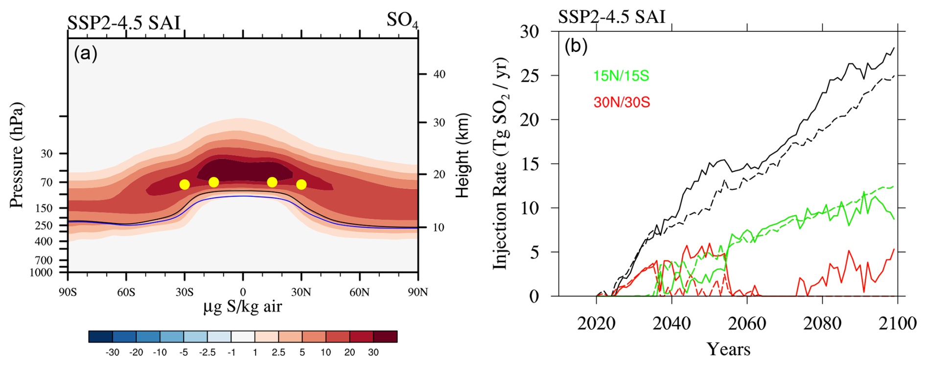
Figure 2 (a) Differences of zonally and annually averaged SO₄ concentrations between the SSP2-4.5 SAI experiment in 2080–2099 and the control experiment (SSP2-4.5) in 2020–2030. The lapse rate tropopause is indicated as a black line for the control experiment and a blue line for the SO₂ injection cases. Yellow dots are the locations of injection. (b) Annual injection rates of SO₂ at 15° N and 15° S (green lines) and at 30° N and 15° S (red lines), as well as the total (black lines). Different lines indicate the result of two different ensemble members.

The modified choice of climate targets compared to the previous WACCM6 SAI studies is to produce a symmetric stratospheric aerosol distribution and SAOD in the two hemispheres, requiring more SO₂ injections at 15° N and S and 30° N and S (Fig. 2). Previous studies with 3 degrees of freedom for SO₂ injections show that more injections are often required in one hemisphere to keep the interhemispheric temperature gradient from changing. The details are strongly model-dependent and due to differences in internal feedbacks and sensitivities to increasing GHGs and SAI (e.g., Fasullo and Richter, 2023; Henry et al., 2023). However, differences in the interhemispheric aerosol distribution lead to different chemical (ozone) and dynamical responses and are not desired for multi-model comparisons.

2.2.3 CCMI-2022 senD2-sai and senD2-fix simulations

The CCMI senD2-sai experiment is designed to keep global mean surface temperatures from changing from 2020–2030 conditions, while greenhouse gas concentrations, ODS, and emissions follow the refD2 CCMI future model experiment (see Fig. 1a, red lines). However, instead of including interactive stratospheric aerosols through stratospheric SO₂ injections, it uses the stratospheric aerosol distribution or aerosol properties provided by the SSP2-4.5 SAI experiment starting in 2020. This method has been applied in earlier SAI studies; e.g., three out of six models participating in the GeoMIP G6 experiment used prescribed aerosol distributions (Tilmes et al., 2022). In addition, WACCM6 aerosol optical information was also recently used and imposed in GFDL-ESM4 to perform SAI model experiments (Zhang et al., 2024a). The information provided by WACCM6 results for the CCMI experiment includes 5 d instantaneous zonal mean output of sulfate aerosol concentrations for the three available aerosol modes, surface area density in both the troposphere and stratosphere, effective radius, and aerosol optical depth at 500 nm between 2020 and 2100.

Since some CCMI-2022 models require additional information on aerosol properties available from WACCM6, this dataset is complemented with additional required quantities. In particular, the stratospheric aerosol distribution provided from the WACCM6 SSP2-4.5 SAI simulation does not contain sufficient information, particularly the optical properties extinction coefficient, single-scattering albedo, and asymmetry factor at all the different wavelengths, needed for some CCMI-2022 models. To produce this information, Jörimann et al. (2025) developed a method to produce the required aerosol and optical properties from the provided WACCM6 distribution. In detail, the number density and wet diameter, as well as a fixed half width σ, were used to characterize the size distribution of the three aerosol modes. The half widths are 1.6, 1.6, and 1.2 for the three modes, respectively. Model output temperature and relative humidity fields were used to calculate the water weight percentage of the aerosol particles. With these parameters being known, all three optical properties can readily be calculated and summed up over the three modes using Mie theory for a homogeneous sphere (Bohren and Huffman, 1998), i.e., a liquid aerosol particle. With this method, the optical properties can be given for any wavelength band, making it adaptable to any radiation scheme spectral resolution. The REMAP code and its products are freely available for download from the ETH research collection: https://doi.org/10.3929/ethz-b-000714654 (Jörimann, 2025).

For WACCM6 senD2-sai, the 5 d instantaneous varying stratospheric aerosol distribution can be directly used. For chemical processing, WACCM6 uses the prescribed aerosol surface area density (SAD) (called SAD-AERO) from SSP2-4.5 SAI. This variable ignores the swelling and uptake of nitric acid and water vapor for cooler temperatures below 200 K and only assumes liquid binary solutions. For chemical heterogeneous reactions in the stratosphere, WACCM6 then internally calculates another aerosol SAD variable (called SAD-SULFC) that considers both liquid binary sulfate aerosols and supercooled ternary solutions, as well as two additional SAD variables for polar stratospheric clouds (Kinnison et al., 2007; Solomon et al., 2015). For radiative calculations, WACCM6 uses the 5 d zonal mean mass and wet radius of the three stratospheric aerosol modes from the SSP2-4.5-SAI simulation to derive radiative properties.

In addition, for senD2-sai, instead of using an interactive ocean, climatological SSTs and sea ice values are prescribed using the model-specific 2020–2030 (inclusive) climatology of the corresponding refD2 experiment throughout the senD2-sai simulation length. The prescribed SSTs, therefore, match the SAI temperature target. As a result, only minor global mean surface temperature variations are simulated in senD2-sai due to changes from the atmosphere and land (Fig. 1a, red lines). On the other hand, the feedback from the atmosphere and land changes in the globally averaged precipitation in senD2-sai is significantly lower than in SSP2-4.5 SAI (Fig. 1b, red lines). Details of the difference in surface climate between these two experiments will be discussed in Sect. 3.

While SAI starts in 2025 in senD2-sai, we recommend that models start their simulations in 2020 to adjust to the new background aerosol distribution (see Sect. 2.2). This is desirable since not all models use the same aerosol background conditions for refD2. We further require performing a background aerosol experiment senD2-fix. This experiment is identical to senD2-sai; however, instead of using the time-varying prescribed stratospheric aerosol described above, this experiment repeats background climatological stratospheric aerosol averaged between 2020–2024 (inclusive). This simulation is required to be performed over 2015–2035 (pink lines in Fig. 1a and b) at the least, but it is recommended that it be extended until the end of the century if possible.

3 Prescribed aerosols versus interactive injections

Using WACCM6, we can directly compare the fully interactive SSP2-4.5 SAI experiment results with the senD2-sai simulation with prescribed stratospheric aerosol and fixed SSTs and sea ice in the same model framework. Differences between the two experiments are only due to the experimental setup discussed above, while information from the derived stratospheric aerosol distribution, namely surface area density (SAD), aerosol mass, and mode radius provided from SSP2-4.5 SAI, is adopted without any required adjustments, described in Sect. 2.5. In the following, we compare the results of these two SAI experiments, SSP2-4.5 SAI and senD2-sai, for the future 2080–2099 period against their respective control simulation from SSP2-4.5 and senD2-fix, respectively, for the period 2020–2030 (see Table 1).

3.1 Stratospheric chemistry and dynamics response to SAI

The effects of SAI on stratospheric temperature, dynamics, and chemistry across multiple models have been discussed in previous papers (e.g., Niemeier et al., 2020; Visioni et al., 2021a; Tilmes et al., 2022; Bednarz et al., 2023) and are briefly reviewed below. Here, we mainly focus on the differences between the fully interactive model experiment and those using prescribed stratospheric aerosol and SSTs and sea ice.

Figure 3 (a–c) Differences of zonally and annually averaged surface area density (SAD-AERO; see text for more detail) between SSP2-4.5 SAI in 2080–2099 and the control experiment (SSP2-4.5) in 2020–2030 (a), between senD2-sai and the control experiment (senD2-fix) in 2020–2030 (b), and between SSP2-4.5 SAI and senD2-sai in 2080–2099 (c). (d–i) Differences of zonally averaged temperature for December, January, and February (d–f) and June, July, and August (g–i) between SSP2-4.5 SAI in 2080–2099 and the control experiment (SSP2-4.5) in 2020–2030 (left), between senD2-sai and the control experiment (senD2-fix) in 2020–2030 (middle), and between SSP2-4.5 SAI and senD2-sai in 2080–2099 (right). The lapse rate tropopause is indicated as a black line for the control experiment and a blue line for the SAI cases. Areas of non-significant difference at the 95 % level to the control are marked as small black dots.

By construction, SAD-AERO values simulated in SSP2-4.5 SAI and prescribed in refD2-sai are similar in the stratosphere (as shown in Fig. 3a, b, and c, described in Sect. 2.4), with slightly smaller values in the extratropical lower stratosphere in SSP2-4.5 SAI. In the interactive aerosol simulation, SAD is calculated for each grid point, while SAD in the prescribed experiment uses zonal mean values, likely leading to slight differences. Furthermore, in the interactive stratospheric aerosol simulation, stratospheric aerosols are transported into the troposphere and eventually deposited at the surface. In contrast, for the prescribed stratospheric aerosol experiment, the model zeroes out the prescribed aerosol distribution and SAD below the tropopause. In WACCM6, the tropopause is internally calculated via the WMO lapse rate calculation for latitudes lower than 50° N and S. It uses climatological tropopause values for latitudes larger than 50° N and S due to difficulties deriving the tropopause at all times in higher latitudes, which is generally lower than the internal model tropopause. This feature results in the abrupt change in SAD around 50° N and S around the tropopause (Fig. 3c). Therefore, the prescribed SAD in senD2-sai reaches lower vertical levels than indicated by the internally calculated tropopause in Fig. 3, blue and black lines. The small differences in SAD-AERO in the troposphere and stratosphere are not expected to largely impact stratospheric heterogeneous chemistry. Furthermore, corresponding differences in aerosol mass could result in small differences in the radiative response, as discussed below.

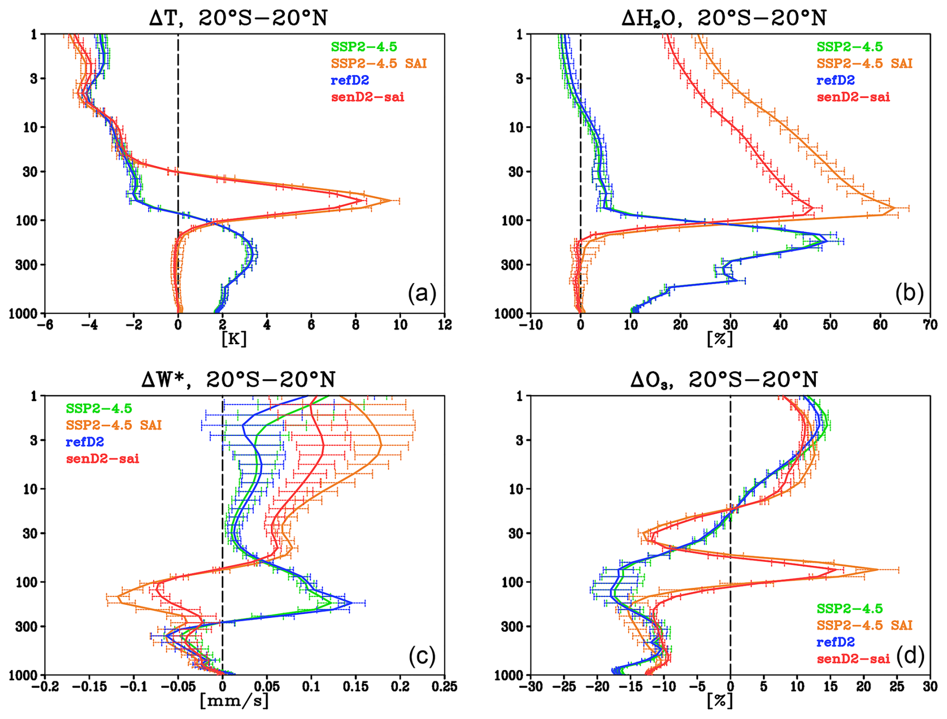
Figure 4 Zonal mean differences between 20° N and 20° S between 2080–2099 and control conditions (2020–2030) for temperature (a), water vapor (b), transformed Eulerian mean vertical velocity (w^⋆) (c), and ozone (d), for the different experiments.

Changes in temperature and other variables result from the increasing GHG concentration and changes in ODS levels between 2080–2099 and 2020–2030 and SAI. The strong decrease in temperature in the upper stratosphere for both SAI experiments compared to the control results from higher GHGs in 2080–2099 compared to 2020–2030 (Fig. 3d, e, g, and h). On the other hand, SAI increases temperatures in the tropical lower stratosphere by 5–10 K and in the summer polar lower stratosphere by 2–5 K, mainly due to the absorption of longwave and shortwave radiation from the elevated sulfate mass (Fig. 3d, e, f, g, h, and i; Fig. 4a). The resulting increase in tropical tropopause temperatures significantly increases water vapor in the stratosphere (Fig. 4b), which counters some of the surface cooling effects of SAI. Increasing stratospheric water vapor with SAI also impacts stratospheric chemistry via changes in the reactive-hydrogen ozone-destroying cycle (e.g., Tilmes et al., 2018b; Bednarz et al., 2023; Wunderlin et al., 2024).

Comparisons between senD2-sai and SSP2-4.5 SAI compared to the control show stronger warming of up to 1 K in SSP2-4.5 SAI in the lower tropical stratosphere (Fig. 4a). The stronger warming around and slightly below the tropopause in SSP2-4.5 SAI is consistent with a larger sulfate mass near the tropical tropopause, as discussed above. However, the stronger warming in SSP2-4.5 SAI compared to senD2-sai around 70 hPa (Fig. 3, right panels) cannot be explained by the small differences in the aerosol mass, since aerosol heating shows a local response (Richter et al., 2017). In contrast, the simulated stronger temperature increase in the coupled vs. the constrained experiment is more likely related to the stronger concurrent coupling with the dynamical changes, in particular the tropical upwelling (as illustrated by the vertical component of the transformed Eulerian mean (TEM) circulation, w^⋆), as well as related changes in ozone in this region (Fig. 4), as explained in the following.

SAI impacts the Brewer–Dobson circulation (BDC) (driven by wave forcing described by the TEM), primarily because of the aerosol-induced lower stratospheric heating and reduction of incoming solar radiation impacting atmospheric static stability in both the troposphere and stratosphere, as well as changing zonal winds, which modulate planetary wave propagation and breaking (e.g., Tilmes et al., 2018b; Bednarz et al., 2023). The result is a weakening of the tropical upwelling in the upper troposphere and lower stratosphere and the associated weakening of the shallow branch of the BDC (Fig. 4c). The increase in the upwelling in the mid-to-upper stratosphere above the sulfur injection location, on the other hand, is indicative of an acceleration of the deep branch of the BDC. In SSP2-4.5 SAI, the slightly stronger warming in the tropical lower stratosphere compared to senD2-sai is also consistent with a stronger weakening of the tropical upwelling below the SAI injection location. This is indicative of a generally stronger response in the interactive aerosol simulation than in those with prescribed aerosols. In addition, the reduced upwelling results in reduced tropospheric ozone-poor air entering the lower stratosphere, resulting in more ozone and therefore more heating, which amplifies the heating differences between SSP2-4.5 SAI and senD2-sai. The difference in upwelling between the two experiments may be caused initially by the slightly warmer temperatures around the tropopause (due to more aerosol mass) in the interactive model run. Finally, SAI-induced differences in vertical advection and resolved wave drag (illustrated by the changes in the Eliassen–Palm flux divergence in Fig. A2) can affect the Quasi-Biennial Oscillation (e.g., Richter et al., 2017, 2018), which will be investigated in future studies.

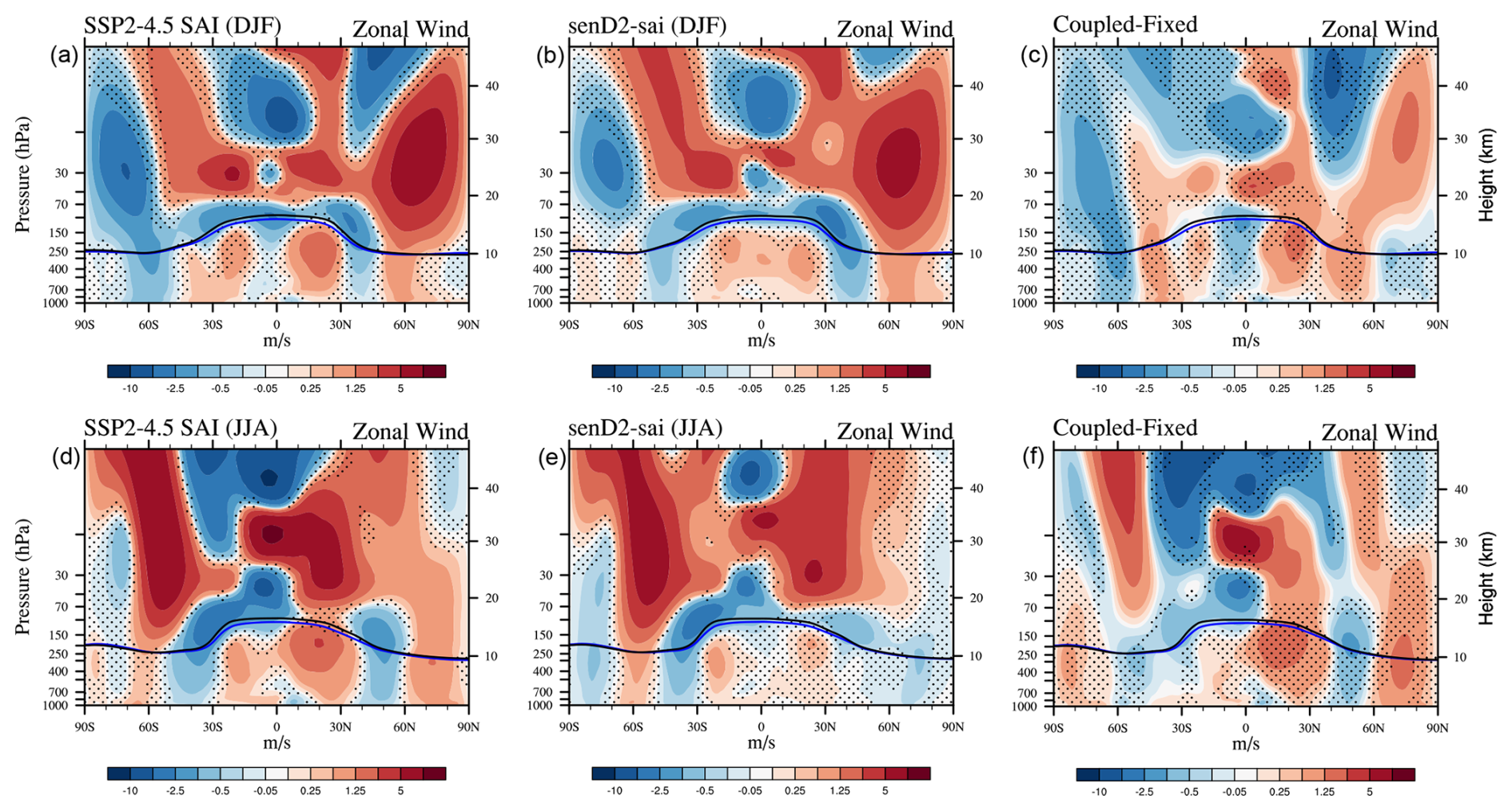
Figure 5 Differences of zonally averaged zonal wind velocity for December, January, and February (a–c) and June, July, and August (d–f) between SSP2-4.5 SAI in 2080–2099 and the control experiment (SSP2-4.5) in 2020–2030 (left), between senD2-sai and the control experiment (senD2-fix) in 2020–2030 (middle), and between SSP2-4.5 SAI and senD2-sai in 2080–2099 (right). The lapse rate tropopause is indicated as a black line for the control experiment and a blue line for the SAI cases (left and middle panels). Areas of non-significant difference at the 95 % level to the control are marked as small black dots.

The simulated temperature reductions in the winter polar lower stratosphere are also impacted by dynamical changes, namely a stronger polar vortex under SAI (e.g., Tilmes et al., 2022), shown for both Arctic and Antarctic polar vortices (Fig. 5). In general, changes in polar vortex strength are associated with changes in BDC and polar downwelling, which modulates the strength of adiabatic warming in winter high latitudes. In addition, increased GHG and decreased ODS levels (comparing future vs. present-day conditions) likely contribute to the simulated strengthening of the polar vortex shown in Fig. 5 (WMO, 2022, and references therein; Butchart et al., 2010; McLandress et al., 2010; Karpechko et al., 2022). Temperature differences between SSP2-4.5 SAI and senD2-sai in high latitudes are small, with a significantly weaker polar vortex in both hemispheres polewards of 60° in the interactive SSP2-4.5 SAI simulation. This may be in part a result of ocean coupling countering the stronger surface pressure reduction simulated over the winter pole in senD2-sai, discussed below.

Changes in high latitudes are further coupled to large-scale changes in the BDC. ESMs project future speeding up of the BDC under global warming as the result of GHG-induced changes in surface and atmospheric temperatures impacting wave generation, propagation, and breaking (e.g., Butchart et al., 2010; Hardiman et al., 2014; Abalos et al., 2021; Keeble et al., 2021). The stronger increase in w^⋆ in the stratosphere above the injection locations in SSP2.4-5 SAI is aligned with the stronger heating in the tropical lower stratosphere compared to senD2-sai, and it may be further amplified by increased wave-driven changes initiated in the troposphere. Furthermore, SSP2-4.5 SAI shows stronger zonal mean wind changes in the tropical troposphere – most pronounced in the NH (Fig. 5). The weakening of the subtropical tropospheric jet is reaching all the way down to the surface in SSP2-4.5 in both hemispheres, while the response is much weaker in senD2-sai, in particular for the NH. These differences point to the importance of ocean feedback in SSP2-4.5 SAI, while some differences may also result from the differences in near-surface temperature response in the two experiments, as further discussed in Sect. 3.2.

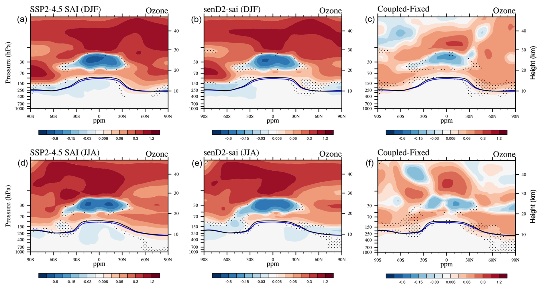
Figure 6 Differences of zonally averaged ozone mixing ratios (ppm) for December, January, and February (a–c) and June, July, and August (d–f) between SSP2-4.5 SAI in 2080–2099 and the control experiment (SSP2-4.5) in 2020–2030 (left), between senD2-sai and the control experiment (senD2-fix) in 2020–2030 (middle), and between SSP2-4.5 SAI and senD2-sai in 2080–2099 (right). The lapse rate tropopause is indicated as a black line for the control experiment and a blue line for the SAI cases. Areas of non-significant difference at the 95 % level to the control are marked as small black dots.

The simulated changes in stratospheric ozone between 2080–2099 and 2020–2030 in the SAI runs, as shown in Fig. 6, are due to the combined effects of increasing GHGs, decreasing stratospheric halogen levels, and SAI forcings, resulting in both chemical and dynamical changes. The direct effect of SAI on ozone is illustrated in Fig. A3, comparing SSP2-4.5 SAI minus SSP2-4.5 and senD2-sai minus senD2-fix for future conditions. In general, the interplay of chemical vs. dynamical drivers of ozone depends on location and season (e.g., WMO, 2022). Compared to the present day and independent of SAI, the most pronounced change in ozone mixing ratios in future scenarios is the substantial increase in ozone concentration in both the upper stratosphere and the polar regions, dominated by reduced halogen content in 2080–2099 compared to 2020–2030. In addition, the increase in GHG concentrations results in a cooling of the upper stratosphere and, consequently, a slowing of reactive ozone-depleting cycles (Haigh and Pyle, 1982). Furthermore, adding SAI increases ozone in the mid-to-upper stratosphere due to increased nitrogen pentoxide hydrolysis, reducing nitrogen oxide and the resulting catalytic ozone loss. The decrease in ozone in the middle tropical stratosphere at ≈ 30 hPa and increases in the lower tropical stratosphere are, for the most part, dynamically driven by the acceleration of the tropical upwelling above the SAI injection location and the enhanced transport of lower ozone concentrations into this region, as well as the reduced upwelling below SAI injections with reduced transport of ozone-poor tropospheric air masses above the tropopause region, as discussed above (Fig. 4c and d). In addition, enhanced stratospheric water vapor (Fig. 4b) due to the warming of the tropical tropopause increases the reactive-hydrogen ozone loss cycle. Finally, reductions in ozone in the Southern Hemisphere (SH) polar lower stratosphere with SAI are the result of increased heterogeneous reactions with increased SAD and a stronger polar vortex (Fig. 5), which is countered by the increase in ozone due to reductions in stratospheric halogen burden under decreasing ODS levels as well as due to the SAI-induced changes in ozone transport and BDC compared to the present day (WMO, 2022).

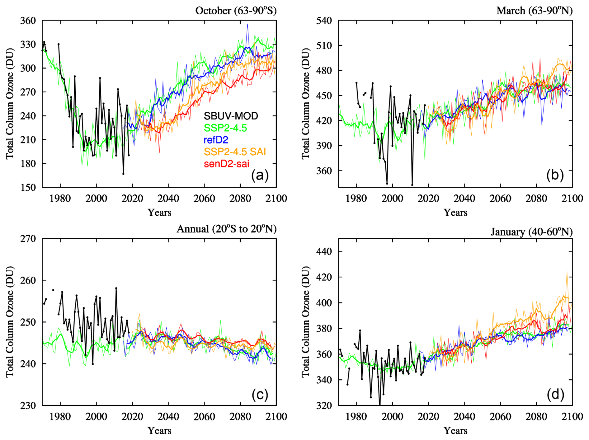
Figure 7 Ensemble mean (thin lines) and a 5-year running mean of the ensemble mean (thick lines) of total column ozone for October between 63–90° S (a), March between 63–90° N (b), annual average between 20° S–20° N (c), and January between 40–60° N (d) for different model experiments. Total column ozone observations from the Solar Backscatter Ultraviolet (SBUV) Merged Ozone Data Set (MOD) (Frith et al., 2017) are shown as black lines. The 5-year running mean has been added to better visualize differences between experiments.

Comparison between changes in SSP2-4.5 SAI and senD2-sai reveals larger magnitudes of the tropical ozone anomalies, in particular, a stronger increase of ozone above the tropical tropopause in the coupled runs (Fig. 6c and f and Fig. A3), in accord with the concurrent stronger lower stratospheric heating and changes in tropical upwelling discussed above. Significant differences between SSP2-4.5 SAI and senD2-sai also occur in the polar regions, including more pronounced reductions of SH polar ozone in senD2-sai. Differences in the polar lower stratospheric ozone anomalies between the coupled and constrained simulation could also be related to slightly lower aerosol SAD changes in the coupled run (Fig. 3a, b, and c), which reduces the amount of halogen activation and chemical ozone loss. In addition, higher polar ozone concentrations in SSP2-4.5 SAI are aligned with the greater changes in the SAI-induced BDC, due to the stronger tropical stratospheric heating in the coupled run and potentially stronger wave-driven changes arising from ocean feedbacks. Resulting differences, particularly in polar ozone concentrations, affect the evolution of total column ozone (TCO) after 2060 (Fig. 7).

In summary, the stratospheric ozone response to SAI in the prescribed vs. interactive (fully coupled) aerosol simulation is overall similar. Minor differences in the responses for the different model setups in TCO in the future are expected due to differences in the ODS between SSP2-4.5 and refD2, resulting in larger values in SSP2-4.5 for the SH winter polar region (Fig. 7a). Differences in the SAI-induced changes are due to the stronger tropical lower stratospheric heating and the resulting impacts on zonal winds and BDC in a coupled simulation. In addition, climate feedbacks resulting from the coupling to SSTs and sea ice in SSP2-4.5 SAI affect dynamical changes in the stratosphere, including enhanced induced wave activities in the troposphere that strengthen the BDC and weaken the polar vortex. These changes may be in part driven by the El Niño-like response in the tropical Pacific and its teleconnections, as well as uneven near-surface temperature changes in the coupled simulation (see Sect. 3.2). These combined differences result in a slightly larger TCO in the SH polar ozone hole for future simulations without SAI and a slightly smaller SAI-induced reduction in TCO in the interactive simulation. By the end of the experiment, SAI-induced changes in both SSP2-4.5 SAI and senD2-sai are around 10–20 DU after 2070 (Fig. 7a). In the NH winter polar region, the increase in TCO is consistent in all four simulations, with a slightly larger increase of TCO in SSP2-4.5 SAI after 2080, consistent with the stronger wave activity in that run (Fig. 7b). Similarly, TCO shows a stronger increase in the interactive simulation in January NH mid-latitudes reaching up to 10 DU (Fig. 7d). In the tropics, the slight SAI-induced increase in TCO of around 3 DU by the end of the simulation is consistent for both experiments and counters some of the TCO decline in the future without SAI (Fig. 7c). Since the discussed changes between the prescribed and interactive experiment are similar, senD2-sai is expected to be suited to study the effects of SAI on stratospheric chemistry and dynamics for multi-model comparison studies. However, the missing feedback from ocean and sea ice in senD2-sai leads to an underestimation of the dynamical response. This represents a caveat of using a less interactive setup to study the effects of SAI on ozone.

3.2 Tropospheric and surface climate response to SAI

In an interactive model simulation (SSP2-4.5 SAI), the feedback from the ocean plays a dominant role in the tropospheric and surface climate response to SAI beyond the effects on stratospheric dynamics (discussed above). Differences between the surface climate response between SSP2-4.5 SAI and senD2-sai are analyzed in detail in the following. Changes in tropospheric and surface climate for hemispherically symmetric sulfur injections in WACCM6, including near-surface air temperature and precipitation patterns, have been discussed in detail by Zhang et al. (2024b) and Bednarz et al. (2023). Here, we focus on regional differences between the fully coupled SSP2-4.5 SAI and prescribed senD2-sai simulations to isolate the contributions of the dynamical influence via the stratosphere induced by the stratospheric aerosols and feedbacks induced by the coupling with the ocean.

In SSP2-4.5 SAI, mean global near-surface air temperatures have been successfully maintained at the levels corresponding to the target 2020–2030 climate (Fig. 1a). However, the experiment produces a significant overcooling in the Northern Hemisphere of up to 2 °C in a zonal mean and a smaller residual warming of around 0.5 °C in the Southern Hemisphere high latitudes (Fig. 8a). The reason for the uneven cooling in WACCM6 under equal sulfur injections in both hemispheres with SAI (per design) is the model-specific sensitivity to elevated GHG concentrations and SAI. These include adjustments in the SH clouds and coupling with the Atlantic Meridional Overturning Circulation (AMOC), which have yet to be further explored (Fasullo and Richter, 2023). In contrast, the prescribed aerosol experiment, senD2-sai, successfully minimizes changes in zonal mean near-surface air temperatures due to the use of the climatological SSTs and sea ice fixed to 2020–2030 conditions.

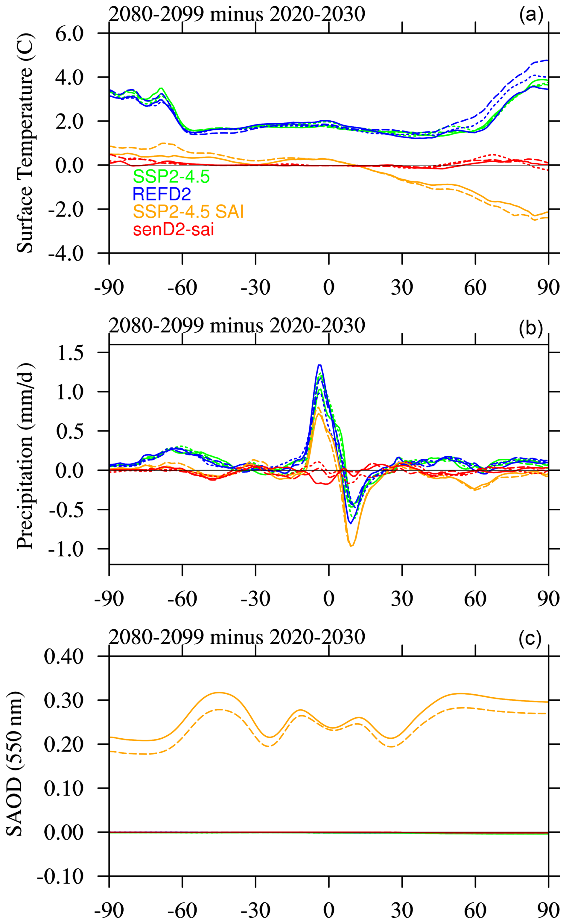
Figure 8 Zonal mean differences between 2080–2099 future experiments and 2020–2030 control experiments for the available ensemble members (different line styles) (see Table 1) for near-surface temperature (a), precipitation (b), and stratospheric aerosol optical depth (SAOD) (c).

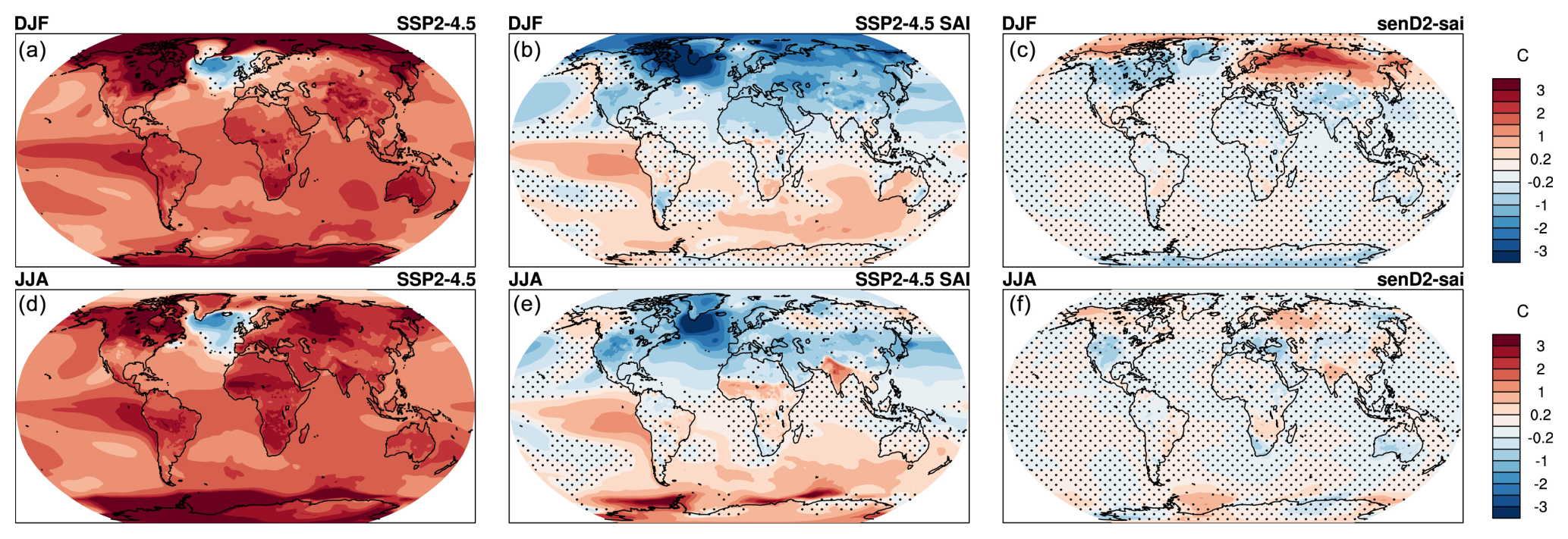
Figure 9 Ensemble-mean differences between 2080–2099 future experiments and 2020–2030 control experiments for near-surface temperature in December, January, and February (a–c) and June, July, and August (d–f) for SSP2-4.5 (left), SSP2-4.5 SAI (middle), and senD2-sai (right). Areas of non-significant difference at the 95 % level to the control are marked as small black dots.

The SSP2-4.5 future climate scenario (Fig. 9a and d) and refD2 (Fig. A4) regional temperature and precipitation changes look almost identical. Future scenarios without SAI show very strong increases in near-surface temperature and a significant reduction of surface temperatures in the North Atlantic region. This response has been discussed in different studies and is due to the projected decline in the strength of AMOC with increasing atmospheric GHG concentrations (e.g., Tilmes et al., 2020; Zhang et al., 2024b; Li et al., 2023). SSP2-4.5 SAI shows a significant NH cooling (Fig. 9b and e). The symmetric injection in both hemispheres using SAI has been shown to counter the weakening of the AMOC due to climate change in WACCM6 (Zhang et al., 2024b).

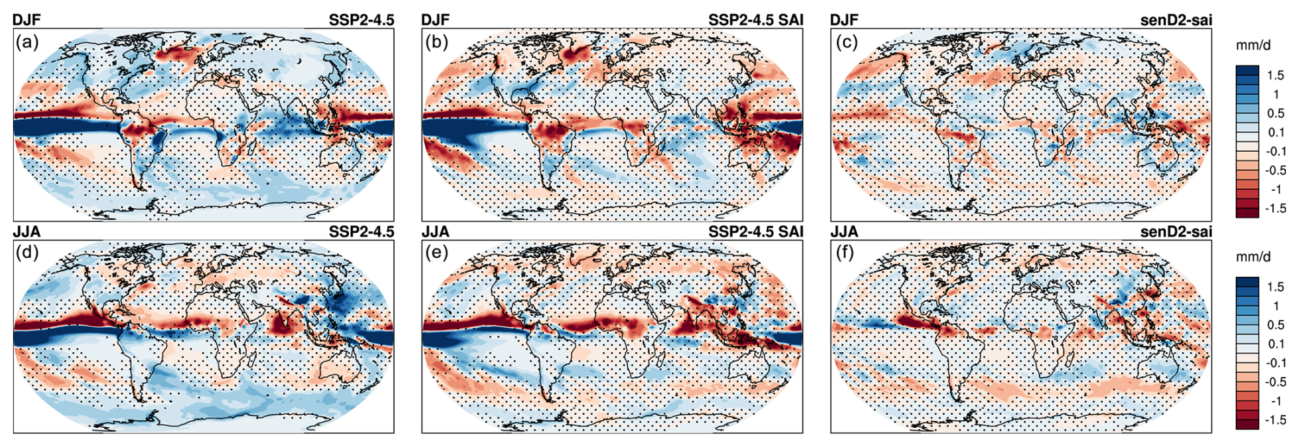
Figure 10 Ensemble-mean differences between 2080–2099 future experiments and 2020–2030 control experiments for precipitation in December, January, and February (a–c) and June, July, and August (d–f) for SSP2-4.5 (left), SSP2-4.5 SAI (middle), and senD2-sai (right). Areas of non-significant difference at the 95 % level to the control are marked as small black dots.

Significant relative warming occurs in the equatorial eastern Pacific in the SSP2-4.5 SAI experiment, similar to the El Niño pattern, and projects on a positive phase of the El Niño–Southern Oscillation (ENSO) (Trenberth, 2020). This response is likely driven by the weakening of the Walker circulation (Bednarz et al., 2023) as a result of the increase in tropical stability due to the heating of the lowermost stratosphere that suppresses tropical convection (Simpson et al., 2019; Malik et al., 2020; Banerjee et al., 2021). However, the exact mechanisms driving this under SAI are yet to be explored (Rezaei et al., 2023). In general, changes in ENSO variability are important in modulating local climate in the tropical Pacific region and, via various teleconnections, can impact the atmosphere globally. For the northern Pacific, changes in the meridional temperature gradients associated with the positive ENSO phase tend to strengthen the subtropical tropospheric jet, while increased tropospheric wave activity acts to deepen the Aleutian low pressure, influencing near-surface air temperature and precipitation patterns in western North America and northeast Asia (Domeisen et al., 2019; also Figs. 9–10). The enhanced tropospheric wave activity under the positive ENSO phase can also enter the stratosphere, acting to strengthen BDC and weaken polar jets (discussed in Sect. 3.1). By design, the constrained senD2-sai experiment does not show any near-surface air temperature changes in the equatorial Pacific and, thus, El Niño-like teleconnections with tropospheric temperatures, winds, and surface pressure and precipitation patterns.

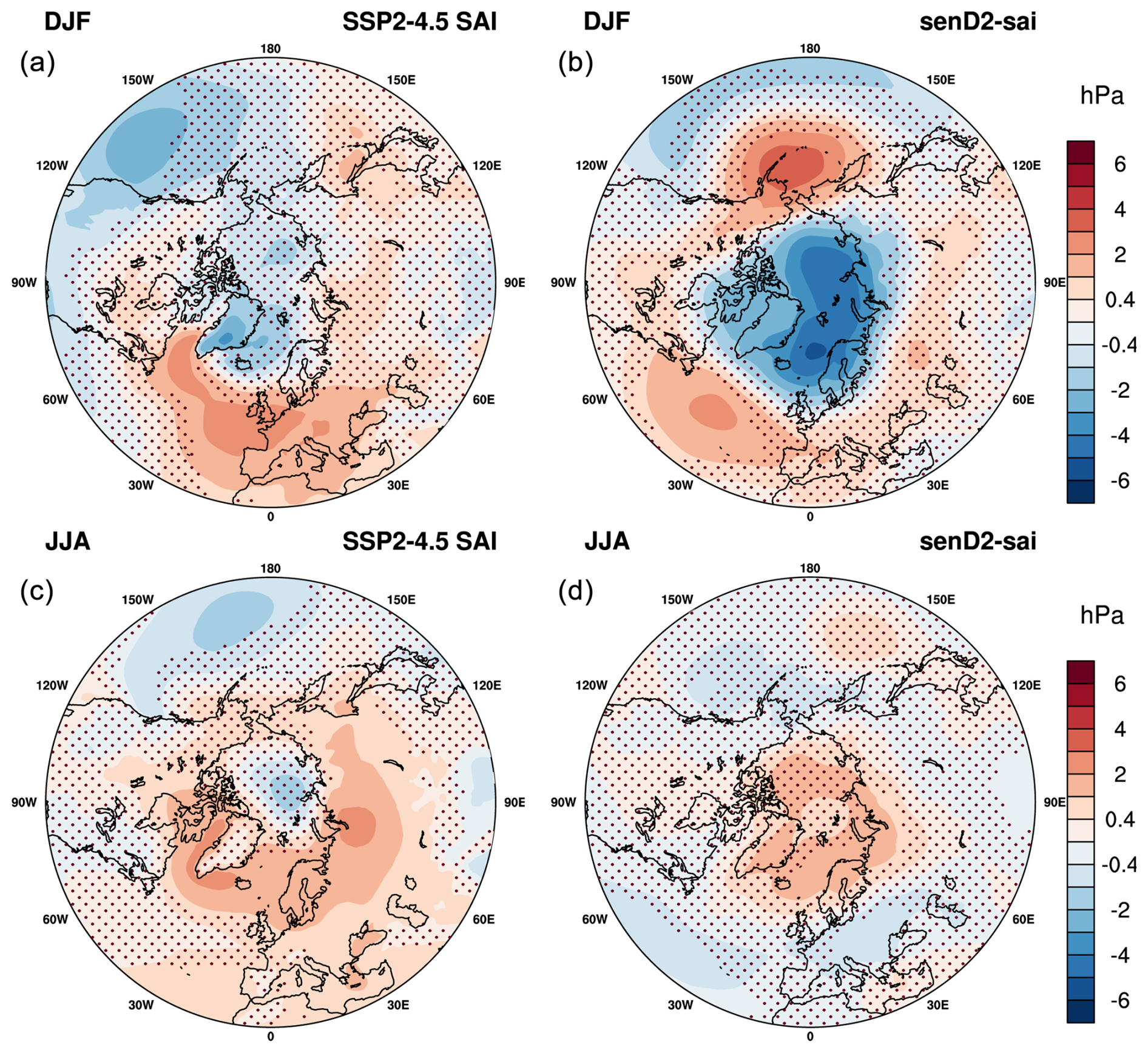
Figure 11 North polar view of ensemble-mean differences between 2080–2099 future experiments and 2020–2030 control experiments for sea-level pressure in December, January, and February (a, b) and June, July, and August  (c, d) for SSP2-4.5 (a, c),​​​​​​​ and senD2-sai (b, d). Areas of non-significant difference at the 95 % level to the control are marked as small black dots.

Differences of near-surface temperature in senD2-sai, Fig. 9c, show a robust winter warming over Eurasia and cooling of the North Atlantic and Greenland. In addition, some significant cooling occurs over central Asia and India. The SAI-induced strengthening of the wintertime stratospheric NH polar vortex can propagate down to the surface, resulting in a pattern of sea-level pressure changes in the North Atlantic projecting onto a positive phase of the North Atlantic Oscillation (NAO), i.e., a significant reduction in sea-level pressure over the Arctic region and a significant increase south of it (Fig. 11b) (Banerjee et al., 2021; Jones et al., 2021; Wunderlin et al., 2024). The described temperature responses in the NH in senD2-sai are a typical signal of the positive NAO. They are also associated with changes in precipitation consisting of drying over southern Europe and wettening over northern Europe (Fig. 10c and f) as storm tracks shift northward, as also discussed in earlier studies (e.g., Haywood et al., 2022; Bednarz et al., 2023). The small but statistically significant cooling in the North Atlantic near Greenland is simulated in senD2-sai despite any changes in SSTs found in the coupled SSP2-4.5 SAI run. Therefore, we conclude for the interactive SSP2-4.5 SAI experiment that besides changes in AMOC, some of the cooling in the North Atlantic has been induced by the stratosphere–troposphere coupling response to SAI, as SSP2-4.5 SAI also shows the positive NAO sea-level pressure pattern (Fig. 11). Furthermore, the sea-level pressure response in senD2-sai is zonally symmetric in origin, with midlatitude sea-level pressure increasing not only in the Atlantic but also in the Pacific Aleutian Low region. This is unlike the negative sea-level response, i.e., strengthening of the Aleutian Low, simulated in SSP2-4.5 SAI discussed above, where teleconnections with the ocean variability dominated the response in the Pacific region.

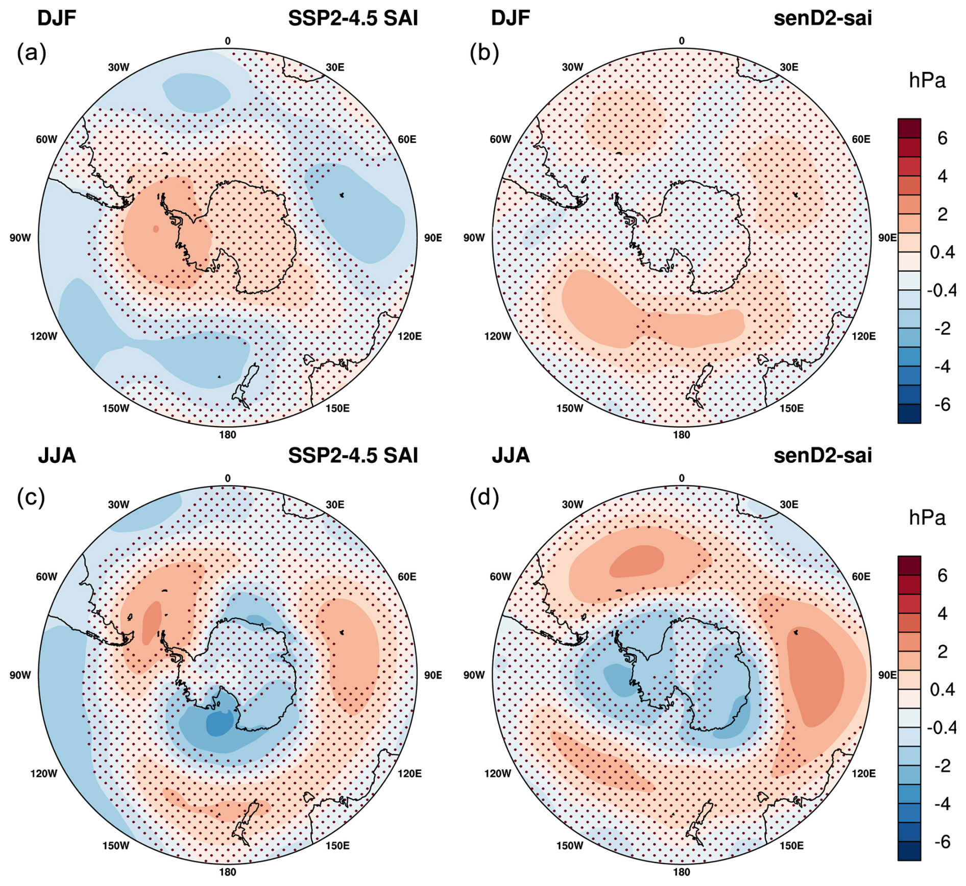
Figure 12 South polar view of ensemble-mean differences between 2080–2099 future experiments and 2020–2030 control experiments for sea-level pressure in December, January, and February (a, b) and June, July, and August (c, d) for SSP2-4.5 (a, c),​​​​​​​ and senD2-sai (b, d). Areas of non-significant difference at the 95 % level to the control are marked as small black dots.

Analogous to what happens in the NH, changes in the strength of the SH stratospheric polar vortex can also be coupled with surface variability, and in this case, this modulation occurs via changes to the Southern Annular Mode (SAM). In both SSP2-4.5 SAI and senD2-sai, the strengthening of the Antarctic polar vortex in austral winter (JJA) results in reduced sea-level pressure over the Antarctic continent and an increase in sea-level pressure over the Southern Ocean (Fig. 12) – a pattern similar to the positive phase of SAM. This response is slightly more significant in senD2-sai than in SSP2.4-5 SAI and, therefore, directly induced by the stratospheric top-down influence. The fixed SST experiment thus supports the suggestions by Bednarz et al. (2022) that a response caused by SAI-induced stratospheric heating can result in a positive SAM. In austral summer, however, while senD2-sai still shows a suggestion (albeit not strongly statistically significant) of a positive SAM-like response, the coupled SSP2-4.5 SAI shows the opposite sign response, i.e., an increase in sea-level pressure over the Antarctic and a decrease in mid-latitudes. This corresponds to the negative phase of SAM and is accompanied by a significant weakening of the SH tropospheric winds at 60° S (Fig. 5), which is not reproduced by the senD2-sai experiment. This austral summer negative SAM and weakening of the eddy-driven jet are therefore likely connected to the sea surface temperatures changes in the equatorial Pacific and the El Niño-like response there, resulting in changes in eddy heat and momentum fluxes and tropospheric winds. A similar relationship has also been found from observations and simple modeling studies (L'Heureux and Thompson, 2006). However, an additional stratospheric-induced contribution from the springtime weakening of the vortex can also not be ruled out as the result of the Antarctic ozone increases from reduced ODS and less SAD in SSP2-4.5 compared to senD2-sai (see Sect. 3.1).

Differences in near-surface temperature in JJA in senD2-sai are, for the most part, insignificant, especially in the NH, where the reductions in the subtropical jet are not reaching the surface and, therefore, not significantly affecting near-surface temperatures (Fig. 5f). Other small near-surface temperature changes in JJA in senD2-sai include cooling over southern Europe and the central US, as well as some cooling over South Australia and South Africa, and some warming in northern Europe and Alaska, parts of South Africa, and east of the Antarctic Peninsula. These changes may be related to additional land feedbacks that have to be further explored in multi-model comparison studies.

The SSP2-4.5 and refD2 simulations without SAI show a similar increase in global mean rainfall with increasing near-surface temperatures (Fig. 1b). On the other hand, SSP2-4.5 SAI and senD2-sai show a precipitation reduction compared to the present day, which is significant about 10 years after the start of SAI. This global mean rainfall reduction is slightly stronger in the coupled SSP2-4.5 SAI compared to senD2-sai. Different processes are likely to contribute to this difference, including the slightly stronger SAI-induced heating in the lower stratosphere, resulting in a greater enhancement in tropospheric static stability (Ferraro et al., 2014; Lee et al., 2023), and additional feedback with the ocean, resulting from the uneven interhemispheric cooling and the El Niño-like response, which is only included in the coupled SSP2-4.5 SAI but not in senD2-sai. Furthermore, zonally averaged changes in precipitation show a similar strengthening of tropical rainfall in the SH and a weakening in the NH for both SSP2-4.5 and refD2 simulations without SAI (Fig. 8b). The response indicates a southward shift of the Intertropical Convergence Zone (ITCZ) under rising GHG levels (Fig. A5). The coupled SSP2-4.5 SAI simulations also show a similar tropical precipitation shift compared to the control, with a relative reduction on both sides of the Equator, therefore amplifying the negative values in the NH and reducing the positive values in the SH compared to SSP2-4.5 without SAI compared to the control in 2020–2030. Therefore, symmetric SAI in WACCM6 counters some of the increase in precipitation in the SH tropics but further reduces precipitation in the NH (Fig. 8b). Consistently, SSP2-4.5 SAI simulations project a reduced rainfall increase in JJA in the western Pacific, aligned with the El Niño signal with SAI compared to the control. Such a response is aligned with a weakening of the Hadley circulation under SAI, as identified for similar experiments in (Bednarz et al., 2023). Furthermore, Bednarz et al. (2023) found an eastward shift of the Walker circulation with SAI for 30° N, 30° S injections associated with surface temperature changes in the equatorial Pacific and the resulting reductions in rainfall over the Maritime Continent and Australia, as can also be seen in SSP2-4.5 SAI (Fig. 10).

In general, precipitation changes in senD2-sai are, for the most part, not significant at the 95 % level of the t test. The minimized changes in near-surface air temperatures in senD2-sai compared to SSP2-4.5 SAI, in particular the significant hemispheric asymmetry that was otherwise seen in the coupled ocean SSP2-4.5 SAI run, prevent shifts in the Hadley (and Walker) circulation and thus the associated large-scale shifts in precipitation. The exceptions are the drying over southwest Europe, a wettening of northern Europe in DJF, and a wettening of western Europe and drying of northern Europe in JJA due to the changes in the NAO sea-level pressure patterns (discussed above). Other signatures include increased precipitation over Australia and the ocean at similar latitudes, while a drying occurs in the Southern Ocean. This zonal pattern is a signature of the concurrent poleward shift in the tropospheric eddy-driven jet (Fig. 5) and a positive SAM-like response (Fig. 12) in JJA. Significant reductions in rainfall also occur over central Africa, Venezuela, and Colombia – regions with strong tropical convection that are likely impacted by increased static stability with SAI (Ferraro et al., 2014). Since senD2-sai included fixed SSTs, precipitation changes cannot be a result of any El Niño-like response and its teleconnections and, therefore, are either driven by the top-down dynamical changes and/or induced in part by changes in evaporation induced by the land feedback to SAI.

4 Conclusions

The new CCMI-2022 senD2-sai experiment has been designed for multi-model comparison studies to investigate the effects of SAI on stratospheric chemistry and dynamics. The constrained experimental setup using a prescribed stratospheric aerosol distribution and fixed SSTs and sea ice allows for a process-level understanding of SAI stratospheric responses and their inter-model differences. These differences can be attributed to the resulting impacts on stratospheric chemistry, radiation, and dynamics rather than inter-model uncertainty in the details of SAI aerosol forcing. In addition, the experimental setup removes the uncertainty in ocean processes and feedbacks under SAI by keeping SSTs and sea ice from changing. This setup, therefore, helps to identify changes that result directly from the SAI-induced changes in the stratosphere, while some feedback from the interactive land is also included. While the top-down response from the stratosphere and bottom-up feedbacks from the ocean are not completely additive owing to the two-way coupling between the stratosphere and the troposphere/surface climate, such a decomposition facilitates an improved understanding of the tropospheric response that is directly affected by the SAI dynamical impacts in the stratosphere. The second part of the paper compares the SAI-induced responses in stratospheric dynamics and chemistry between a fully interactive WACCM6 experiment (SSP2-4.5 SAI) and the constrained CCMI-2022 senD2-sai. The purpose of this comparison is twofold. First, we show that simulated SAI dynamical and chemical responses in the stratosphere between the fully interactive and the simplified senD2-sai simulation are similar. This demonstrates the validity of the senD2-sai setup for multi-model comparison studies of stratospheric SAI impacts, including those focused on stratospheric ozone and circulation. We have also shown that some differences between the interactive and constrained responses can arise due to small differences in the details of aerosol properties and distributions. In addition, feedbacks from ocean and sea ice in the interactive experiment impact the wave activity entering the stratosphere and, therefore, change the response to the BDC with SAI. Therefore, quantitative statements have to be considered with a caveat since results, e.g., changes in total column ozone, may not reflect the full complexity of interactions. For example, we find that following the SSP2-4.5 GHG future scenario, the difference in SAI-induced changes in TCO between the interactive and the constrained experiment is only significant after 2060–2070, when SAI injections are relatively large (above 15 Tg SO₂ yr⁻¹) to counter more than 1 °C of near-surface temperature increase.

We further compared differences in near-surface temperatures and precipitation between the fully interactive and constrained SAI experiments. The setup of the WACCM6 interactive simulation to produce the stratospheric aerosol distribution for the CCMI-2022 senD2-sai experiment used symmetric (equal) injections in each hemisphere. This setup resulted in hemispherically close to symmetric aerosol and AOD distribution desired for multi-model comparisons of SAI stratospheric chemistry and dynamics impacts. However, this setup in WACCM6 results in hemispherically unsymmetrical near-surface temperature cooling, which could be linked to model-specific internal adjustments, including cloud and climate feedback (Fasullo and Richter, 2023). In addition, results show significant equatorial warming in the eastern Pacific related to a positive phase of the El Niño–Southern Oscillation and its associated global-scale teleconnections.

We contrast the results with those from senD2-sai. Prescribed SSTs and sea ice prevent ocean feedbacks and remove the potential for an overcooling or undercooling using a prescribed aerosol distribution from a different model (Zhang et al., 2024a). While land surface temperatures are still allowed to change, these are expected to have a minor impact. We support findings from earlier studies, demonstrating that regional SAI-induced surface climate changes connected to the modulations of extratropical modes of variability (NAO in the NH, SAM in the SH) are driven by the top-down influence of stratospheric circulation responses as the result of aerosol-induced stratospheric heating. In contrast to the extratropical changes, any surface climate responses in the tropics in senD2-sai are found to be very small and/or not statistically significant.

Overall, we have shown that the new senD2-sai experiment is well suited to facilitate process-level understanding of the drivers of SAI stratospheric responses and their inter-model differences. Given the uncertainty in the model representation of ocean processes and feedbacks, the constrained CCMI SAI experiment further allows us to isolate the downward influence of SAI via changes in stratospheric dynamics across models while removing contribution from the ocean to the stratospheric variability. Since the in-depth assessment of SAI-induced changes in stratospheric chemistry and aerosols in a multi-model setup is an important mandate by CCMI to support the upcoming WMO assessment, we encourage modeling groups to participate in this important effort.

Appendix A: Supporting figures

This section includes supporting material in the form of additional Figs. A1 to A5, as referred to in the main text.

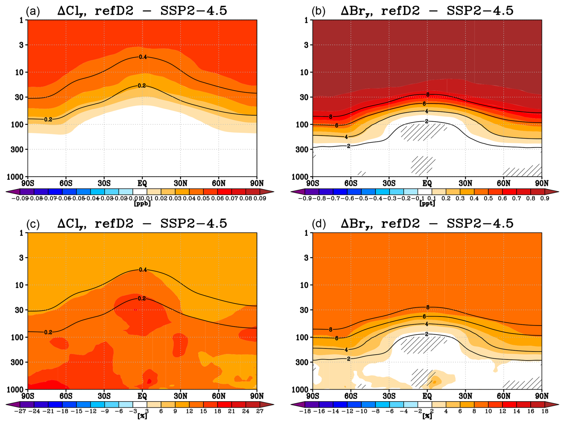
Figure A1 Zonal mean absolute (a, b) and relative (c, d) changes in total chlorine (Cl_y) (a, c) and total bromine (Br_y) (b, d) between refD2 and SSP2-4.5 scenarios for 2080–2099 conditions.

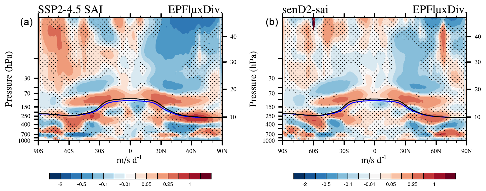
Figure A2 Differences of zonally and annually averaged Eliassen–Palm flux divergence between SSP2-4.5 SAI in 2080–2099 and SSP2-4.5 in 2015–2035 (a) and senD2-sai in 2080–2099 and senD2-fix in 2015–2035 (b). Areas of non-significant difference at the 95 % level to the control are marked as small black dots.

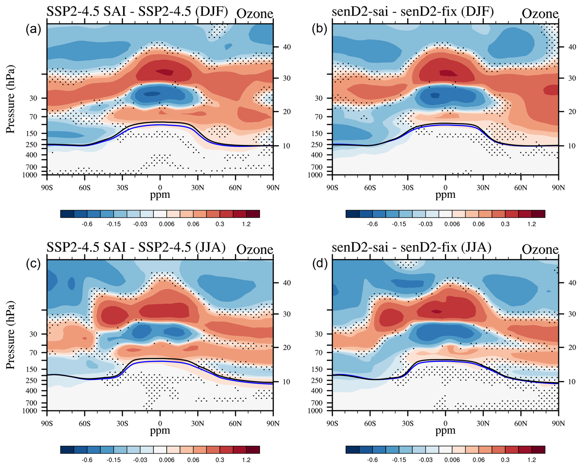
Figure A3 Differences of zonally averaged ozone mixing ratios (ppm) for December, January, and February (a, b) and June, July, and August (c, d) between SSP2-4.5 SAI and SSP2-4.5 (left) and senD2 and senD2-fix (right) in 2080–2099. The lapse rate tropopause is indicated as a black line for the control experiment and a blue line for the SAI cases. Areas of non-significant difference at the 95 % level to the control are marked as small black dots.

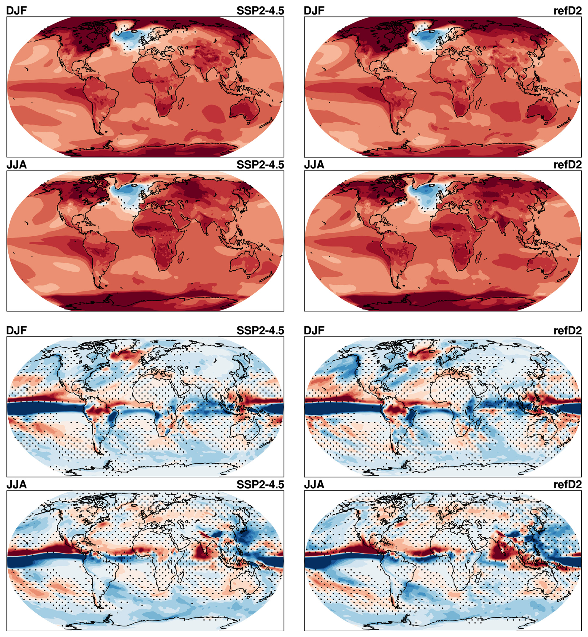
Figure A4 Ensemble-mean differences between 2080–2099 future experiments and 2020–2030 control experiments for near-surface temperature in December, January, and February (first row) and June, July, and August (second row) and for precipitation in December, January, and February (third row) and June, July, and August (fourth row) for SSP2-4.5 (left) and refD2 (right). Areas of non-significant difference at the 95 % level to the control are marked as small black dots.

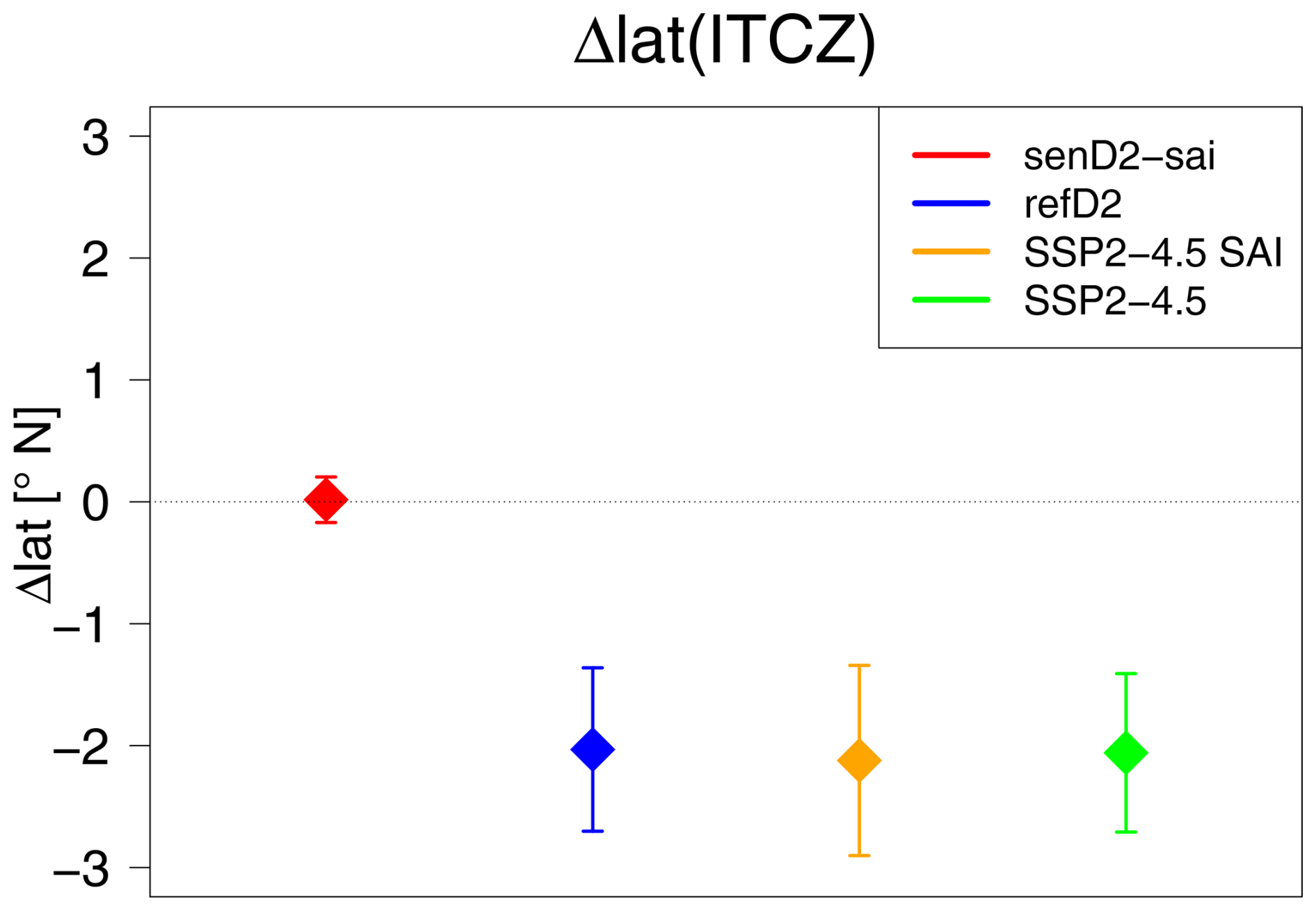
Figure A5 Differences of the annual mean and latitude of the Intertropical Convergence Zone (ITCZ) between 2080–2099 compared to 2010–2030 for different experiments (see legend); the standard error is shown as vertical bars.