Investigating the role of stratospheric ozone as a driver of inter-model spread in CO₂ effective radiative forcing

Addressing the cause of inter-model spread in carbon dioxide (CO₂) radiative forcing is essential for reducing uncertainty in estimates of climate sensitivity. Recent studies have demonstrated that a large proportion of this spread arises from variance in model base-state climatology, particularly the specification of stratospheric temperature, which itself plays a dominant role in determining the magnitude of CO₂ forcing. Here, we investigate stratospheric ozone (O₃) as a cause of inter-model differences in stratospheric temperature, and hence its role as a contributing factor to spread in CO₂ radiative forcing. We use the Norwegian Earth System Model 2 (NorESM2) to analyse the impact of systematic increases and decreases in stratospheric O₃ on the magnitude of 4xCO₂ effective radiative forcing (ERF) and its components. Firstly, we demonstrate that the accurate estimation of instantaneous radiative forcing (IRF) requires the use of host-model radiative transfer calculations. Secondly, we show that a 50 % increase or decrease in the stratospheric O₃ concentration leads to significant differences in the base-state stratospheric temperature, ranging from +6 to −9 K, respectively. These experiments impact IRF primarily due to the influence of the base-state stratospheric temperature on the emission of outgoing longwave radiation, with the spectral overlap of CO₂ and O₃ playing a subsidiary role. However, the impact on IRF does not result in a correspondingly large spread in CO₂ ERF. We conclude that inter-model differences in stratospheric O₃ concentration are, therefore, not predominantly responsible for inter-model spread in CO₂ ERF.

1 Introduction

Effective radiative forcing (ERF) quantifies the top-of-atmosphere (TOA) perturbation to the Earth's energy balance imposed by a forcing mechanism, such as CO₂, aerosols or solar irradiance. It includes the instantaneous radiative forcing (IRF; i.e. the initial radiative response to the perturbation) and the subsequent radiative effect of adjustments in tropospheric and stratospheric temperature, water vapour, surface albedo and clouds, which each cause an impact on TOA radiative fluxes (Myhre et al., 2013; Boucher et al., 2013; Sherwood et al., 2015; Forster et al., 2021).

ERF can be expressed simply (e.g. Chung and Soden, 2015a; Smith et al., 2018) as follows:

$$\begin{array}{}\text{(1)}& \text{ERF}=\text{IRF}+A_{T_{\text{Strat}}}+A_{T_{\text{Trop}}}+A_{{\mathrm{H}}_{\mathrm{2}}\mathrm{O}}+A_{\mathit{\alpha }}+A_{\mathrm{c}}+\mathit{ϵ},\end{array}$$

where ERF is the net (shortwave plus longwave) change in downward TOA flux (W m⁻²); IRF is the direct net change in downward TOA flux (W m⁻²); A_x is the radiative adjustment from stratospheric temperature (T_Strat), tropospheric temperature (T_Trop), water vapour (H₂O), surface albedo (α) and clouds (c); and ϵ represents a non-linear residual term that is typically small (around 10 % of the ERF; Shell et al., 2008).

ERF is used extensively to compare the relative strength of different forcing agents. Historically, quantifying the climate impact of a given agent commonly relied solely on diagnosing its IRF or stratospheric-temperature-adjusted radiative forcing (SARF; e.g. Ramaswamy et al., 2019). However, given that additional so-called “adjustments” develop from the initial radiative perturbation and impact the TOA imbalance, it is also necessary to include them in the radiative forcing framework. Consequently, this has been shown to improve the utility of the radiative forcing metric in predicting global-mean surface temperature change (ΔT_s), ultimately due to a more realistic separation of forcing from surface-temperature-driven feedbacks (e.g. Sherwood et al., 2015; Marvel et al., 2016; Richardson et al., 2019). Adjustments, therefore, form an important component of climate change assessment and necessitate the use of climate model integrations to simulate the radiative response of tropospheric and land surface changes to the TOA energy imbalance, in addition to the traditional diagnostic of IRF or SARF, which can be calculated using offline radiative transfer codes or simplified expressions (e.g. Hansen et al., 1988; Myhre et al., 1998; Etminan et al., 2016; Meinshausen et al., 2020). This makes ERF considerably more computationally expensive to estimate and introduces more model-diversity-driven uncertainty. The use of different methods to calculate ERF further complicates inter-model comparison, with some studies opting to diagnose the forcing from fixed sea surface temperature (SST) and sea ice simulations (Hansen et al., 2005) or, alternatively, by regressing TOA irradiance against global surface temperature change (Gregory et al., 2004; see Forster et al., 2016).

For CO₂, inter-model spread in ERF remains an ongoing issue. Smith et al. (2020a) report a 4xCO₂ ERF range of 7.3–8.9 W m⁻² for 17 CMIP6 (Coupled Model Intercomparison Project Phase 6; Eyring et al., 2016) models contributing to the Radiative Forcing Model Intercomparison Project (RFMIP; Pincus et al., 2016), which aims to achieve accurate characterisation of ERF through consistent diagnosis with the fixed-SST method (Forster et al., 2016). Whilst this spread has been reduced compared to earlier analysis of 13 CMIP5 models (Kamae and Watanabe, 2012; see Smith et al., 2020a, their Fig. 5), identifying and remedying the exact nature of CO₂ ERF diversity is an active area of research (e.g. Soden et al., 2018; Pincus et al., 2016; Smith et al., 2020a). Several studies have shown that model differences in the magnitude of IRF contribute significantly (e.g. Zhang and Huang, 2014; Chung and Soden, 2015b; Andrews et al., 2015), arising either from radiative transfer parameterisation error (e.g. Collins et al., 2006; Pincus et al., 2015) and/or differences in model base-state climatology (Pincus et al., 2020; Jeevanjee et al., 2021). Recently, He et al. (2023) more specifically attributed this base-state dependence to stratospheric temperature. They reported a significant correlation between 4xCO₂ IRF and 10 hPa air temperature in CMIP5 and CMIP6 models, demonstrating that biases in stratospheric temperature play a leading role in causing inter-model CO₂ IRF spread. Given that IRF accounts for around 60 % of CO₂ ERF and that stratospheric cooling is its dominant adjustment (Myhre et al., 2013; Smith et al., 2018), examining potential causes of model differences in stratospheric temperature presents a clear opportunity to further current understanding.

One such cause could relate to stratospheric O₃ – a key constituent in modulating stratospheric temperature. Depending on the treatment of stratospheric chemistry, models adopt a range of methods to generate O₃ fields using either an interactive chemistry scheme, a simplified online scheme or a prescribed pre-simulated dataset. Consequently, the resulting spatial structure and regional distribution of concentrations can differ substantially. Keeble et al. (2021) evaluated long-term O₃ trends in 22 CMIP6 models and found poor agreement in the simulation of pre-industrial total column ozone (TCO), with a variation from 275 to 340 DU between 60° N and 60° S. Further, a ∼ 20 DU range has been observed between 10 of the models that prescribe stratospheric O₃ according to the CMIP6 O₃ dataset (Checa-Garcia, 2018), highlighting that even the model-specific implementation of common input can lead to significant differences in TCO.

Here, we perform idealised experiments (Sect. 2) to investigate the role of stratospheric O₃ as a driver of inter-model diversity in stratospheric temperature, and hence its role as a driver of spread in CO₂ ERF. First, we examine 4xCO₂ ERF and compare our results to previous estimates, with a particular focus on the diagnosis of IRF and T_Strat (Sect. 3). We then investigate the impact of stratospheric O₃ specification on each component of 4xCO₂ ERF (Sect. 4).

2 Models, experiments and methods

We use atmosphere-only simulations from the “medium-resolution” version of NorESM2 (NorESM2-MM; Seland et al., 2020) to calculate ERF following an abrupt quadrupling of CO₂ relative to pre-industrial (1850) conditions (see Text S1 in the Supplement for further details on the model configuration). This model is used to perform a baseline (control) integration and a perturbed (4xCO₂) integration using prescribed SST and sea ice extent climatologies; hence, we use the fixed-SST method to diagnose forcing as recommended by RFMIP (Pincus et al., 2016), whereby ERF is calculated as the difference in TOA net radiative flux between the perturbed and control simulations. Integrations are run for 30 years, with years 6 to 30 used for analysis in Sect. 3. This simulation length was chosen to allow for better comparison of our results against the 30-year NorESM2-MM 4xCO₂ ERF experiments of Smith et al. (2020a).

We perform two further 4xCO₂ ERF experiments in which stratospheric O₃ is increased by 50 % (Strat O₃x1.5) and decreased by 50 % (Strat O₃x0.5) relative to its pre-industrial concentration. Considering the substantial range in pre-industrial TCO noted by Keeble et al. (2021, their Fig. A3), we choose such a large, idealised increase and decrease in an attempt to cover a broader range of stratospheric O₃ than shown by CMIP6 models; thus, any effect on 4xCO₂ ERF would likely be amplified in comparison.

Note that, in each ERF experiment, the O₃ increase (and decrease) is applied to both the control and 4xCO₂ simulation so that the new O₃ field acts exclusively to alter the base-state atmosphere and does not act as a forcing itself. As in the “standard” 4xCO₂ ERF experiment described above, stratospheric O₃ fields are prescribed using zonally averaged 5 d fields derived from the Whole Atmosphere Community Climate Model version 6 from the Community Earth System Model version 2 (CESM2-WACCM6; Gettelman et al., 2019) (Fig. S1 in the Supplement). A linearly varying tropopause (from 100 hPa at the Equator to 300 hPa at the poles) is used to delineate the stratosphere and troposphere (Soden et al., 2008; Smith et al., 2018). O₃ concentrations above this boundary are multiplied by 1.5 and 0.5 to increase and decrease levels by 50 %, respectively. These simulations are run for 15 years to reduce computational expense, with years 6 to 15 of each integration used for analysis (Sect. 4). Table S1 in the Supplement summarises all experiments.

IRF is calculated using the Parallel Offline Radiative Transfer (PORT; Conley et al., 2013) code. This code isolates the radiative transfer scheme employed by NorESM2-MM (i.e. RRTMG; Iacono et al., 2008) to provide stand-alone offline radiation diagnostics. It is used here to perform two sets of radiative transfer calculations for each experiment listed in Table S1: a baseline (control) simulation and a perturbed (4xCO₂) simulation, which are both run using a year's worth of climatology from the corresponding ERF control integration (i.e. the first 12 months of its output). Simulations are then run for 12 months to diagnose the annual-mean IRF as the difference in TOA net radiative flux between the perturbed and control run.

Corresponding radiative adjustments are quantified using radiative kernels (Soden et al., 2008). Summarising the more detailed description given by Smith et al. (2018), these characterise the change in TOA radiative flux ΔR (either shortwave or longwave) following a unit change in a state variable (Δx), e.g. temperature, surface albedo or water vapour. They are constructed by running a climate model's offline radiative transfer code twice, once with a baseline climatology and again with a unit change in x to calculate ΔR. The radiative kernel (K_x) is given by the following:

$$\begin{array}{}\text{(2)}& K_x={\displaystyle \frac{\partial R}{\partial x}}.\end{array}$$

The corresponding adjustment (A_x) is then quantified as follows:

$$\begin{array}{}\text{(3)}& A_x=K_x(x_{\mathrm{p}}-x_{\mathrm{c}}),\end{array}$$

where x_p−x_c represents the difference in x between the perturbed and control atmosphere-only climate model integrations, respectively. Here, A_x is calculated using output from NorESM2-MM with radiative kernels derived from three models: the Community Earth System Model 1–Community Atmosphere Model 5 (CESM-CAM5; Pendergrass et al., 2018), the Hadley Centre Global Environment Model 3-GA7.1 (HadGEM3-GA7.1; Smith et al., 2020b) and the European Centre for Medium-Range Weather Forecasts (ECMWF)-Oslo model (Myhre et al., 2018). We use kernels to calculate all adjustments given in Eq. (1) except for A_c, which cannot be directly calculated from a kernel because the radiative effects of clouds are too non-linear (Soden et al., 2008). To estimate A_c, we calculate the difference between all-sky and clear-sky TOA ERF (i.e. the change in cloud radiative effect; ΔCRE) and then modify this to correct for cloud masking of the clear-sky 4xCO₂ IRF and adjustment response (see Soden et al., 2008, and Smith et al., 2018, 2020a). This differs from alternate approaches used to calculate A_c such as the approximate partial radiative perturbation (APRP) method, which estimates shortwave cloud responses from climate model diagnostics (Zelinka et al., 2014; Smith et al., 2018), and the offline partial radiative perturbation (PRP) method, in which cloud radiative effects are estimated using an offline radiative transfer code and model cloud fields (e.g. Smith et al., 2020a). Additionally, we also use kernels to calculate the adjustment due to surface temperature change ($A_{T_{\mathrm{S}}}$) following Smith et al. (2018), as land surface temperatures are allowed to respond to the forcing in our simulations given the difficulty in prescribing fixed surface temperatures (Forster et al., 2016). Several studies have also followed this approach, whereby the calculation of ERF includes the radiative response of land surface warming or cooling (e.g. Hansen et al., 2005; Forster et al., 2016; Smith et al., 2018, 2020a). Generally, methods that correct for this produce a slightly larger ERF following a CO₂ perturbation (Smith et al., 2020a; Andrews et al., 2021). Subtracting $A_{T_{\mathrm{S}}}$ from the ERF could provide a land-surface-warming-corrected forcing (following Smith et al., 2020a), although we do not calculate this here. Instead, we report the magnitude of $A_{T_{\mathrm{S}}}$ to inspect any change in its value with each O₃ experiment. Further, we use the same tropopause definition as above to delineate $A_{T_{\text{Strat}}}$ and $A_{T_{\text{Trop}}}$.

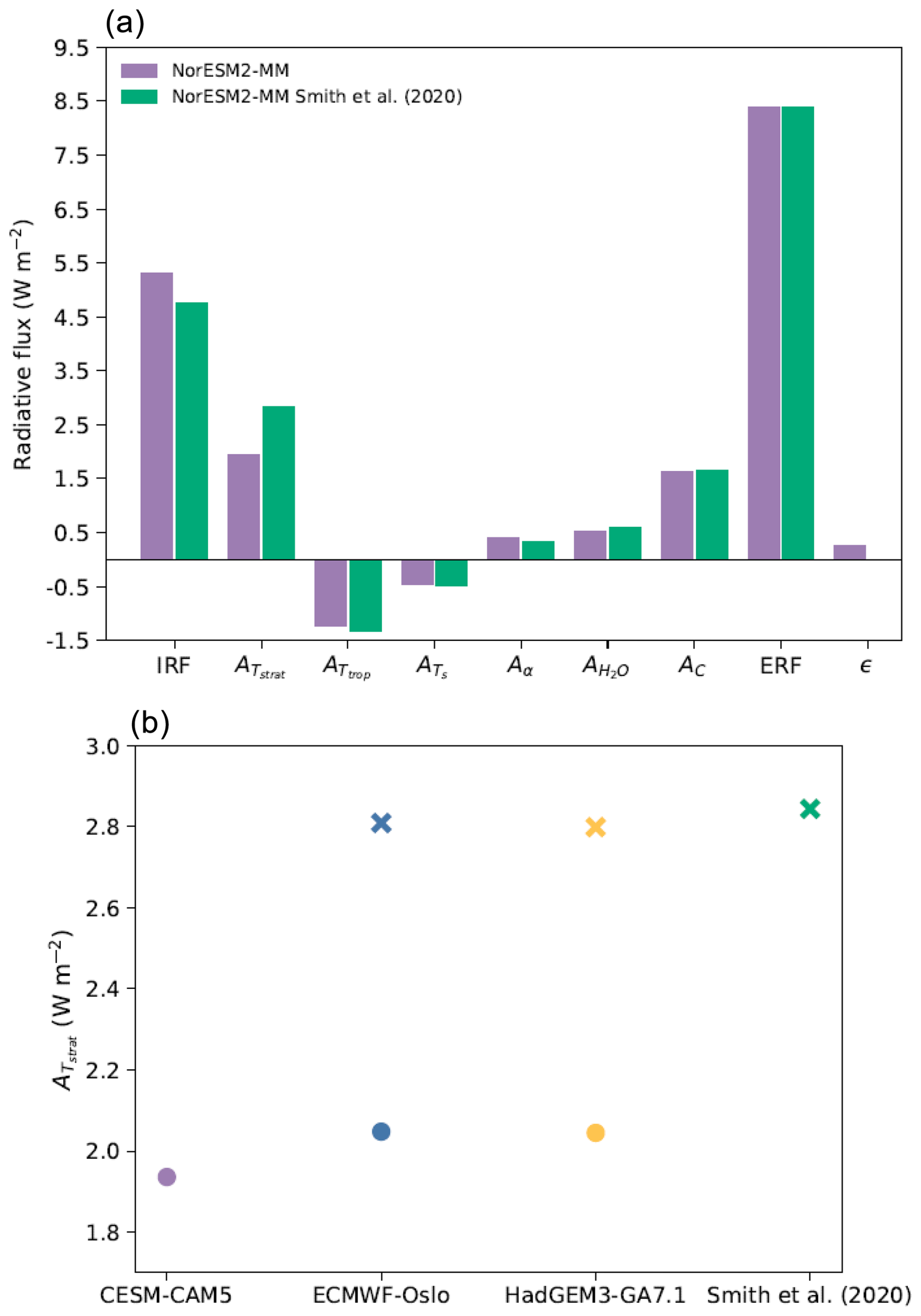
Figure 1 (a) NorESM2-MM 4xCO₂ ERF, IRF, adjustments and the residual term ϵ (purple bars), with IRF calculated using PORT and adjustments diagnosed using the CESM-CAM5 kernels. Green bars show corresponding data from Smith et al. (2020a), whereby the ERF for the same perturbation has been calculated from 30-year simulations of NorESM2-MM with non-cloud adjustments calculated using the HadGEM3-GA7.1 radiative kernels and shortwave and longwave cloud adjustments calculated using the APRP and PRP method, respectively, with IRF estimated as the residual of ERF minus total adjustments; hence, there is no specific ϵ term, as this is aliased into the IRF. (b) Comparison of NorESM2-MM $A_{T_{\text{Strat}}}$ when calculated using different radiative kernels. Filled circles represent $A_{T_{\text{Strat}}}$ calculated following the methodology outlined in Sect. 2, whereby NorESM2-MM output is interpolated onto the given radiative kernel pressure levels but not extrapolated to kernel pressure levels outside of the NorESM2-MM uppermost and lowermost pressures. Crosses represent the magnitude of $A_{T_{\text{Strat}}}$ if such extrapolation is performed using the ECMWF-Oslo (blue cross) and HadGEM3-GA7.1 (yellow cross) kernels along with the value given by Smith et al. (2020a) (green cross, which uses the HadGEM3-GA7.1 kernel).

3 The importance of directly calculating IRF and the dependence of $A_{T_{\text{Strat}}}$ on radiative kernel design

Figure 1a (purple bars) shows the resulting NorESM2-MM ERF, IRF and adjustments. For comparison, corresponding data from the NorESM2-MM 4xCO₂ ERF experiment of Smith et al. (2020a) are also shown (green bars). As expected, the magnitude of ERF is almost equal in each experiment, at 8.40 W m⁻² (purple bar) and 8.38 W m⁻² (green bar). The difference of 0.02 W m⁻² is likely attributable to differences in the time period used to average model output or to the use of alternate initial conditions and computing machine architecture given that all other aspects of simulation design were implemented identically (see Sect. 2 and Sect. 2 of Smith et al., 2020a).

Figure 1a further shows that the magnitude of IRF varies notably, demonstrating a dependence on the diagnostic method of choice. When calculated directly using PORT, the IRF is 0.54 W m⁻² larger than when estimated as the difference between ERF and the sum of adjustments (as in Smith et al., 2020a), comparing 5.30 W m⁻² (purple bar) and 4.76 W m⁻² (green bar). This demonstrates the necessity of using a model's own radiative transfer code to calculate IRF and highlights the possibility for error in studies that derive this forcing as a residual. Directly calculating the IRF also permits the calculation of ϵ (see Eq. 1) to analyse the magnitude of non-linearities that are not accounted for by the kernel-derived adjustments. Our ϵ value (calculated as ERF−IRF−ΣA_x) is 3 % (0.27 W m⁻²) of the ERF (8.40 W m⁻²) and is, therefore, well within the 10 % guideline given by Shell et al. (2008). However, when spectrally split, the shortwave ϵ is 33 % (−0.47 W m⁻²) of the shortwave ERF (1.42 W m⁻²) and works to partially counteract a longwave ϵ of 0.74 W m⁻² (which itself is 11 % of the longwave ERF of 6.98 W m⁻²). This finding also extends to our analysis of the clear-sky 4xCO₂ forcing and adjustments (not shown). These much larger residuals can possibly be explained by the collapse of linear behaviour for a large perturbation like 4xCO₂ (see Jonko et al., 2012; Smith et al., 2020b). We further note the close agreement in A_c, which occurs despite the use of different methods to calculate it. In Smith et al. (2020a), shortwave and longwave A_c are estimated separately using the APRP approach and offline monthly mean PRP calculations, respectively. In our approach, A_c is calculated using the adjusted CRE method (see Sect. 2).

The stratospheric temperature adjustment is strong and positive, as anticipated due to the process of stratospheric cooling following an increase in CO₂ concentration (e.g. Myhre et al., 2013; Smith et al., 2018; Forster et al., 2021). However, there is a clear difference when comparing the value reported here (1.94 W m⁻², purple bar) against Smith et al. (2020a; 2.84 W m⁻², green bar). Because $A_{T_{\text{Trop}}}$ is similar between both experiments (−1.23 vs. −1.32 W m⁻²), it can be deduced that the difference in the magnitude of $A_{T_{\text{Strat}}}$ is not predominantly driven by the choice of the tropopause definition (in Smith et al., 2020a, this is based on the World Meteorological Organization definition of a lapse-rate tropopause). Instead, the difference in $A_{T_{\text{Strat}}}$ stems from the use of different radiative kernels (i.e. CESM-CAM5 vs. HadGEM3-GA7.1) and the method of applying model output in the $A_{T_{\text{Strat}}}$ calculation. For our derivation of $A_{T_{\text{Strat}}}$, we interpolate NorESM2-MM output to the 30 CESM-CAM5 kernel pressure levels, where 3.64 hPa is the highest level. Even though this is a “low-top” kernel, it matches the highest level of NorESM2-MM output, meaning that the use of this kernel in the $A_{T_{\text{Strat}}}$ calculation captures all of the stratospheric cooling occurring in NorESM2-MM following a 4xCO₂ perturbation. Alternatively, Smith et al. (2020a) used the HadGEM3-GA7.1 radiative kernel, which itself has been interpolated from a native vertical resolution of 85 pressure levels (up to around 0.005 hPa) to the standard 19 CMIP6 pressure levels, with an upper bound of 1 hPa. Smith et al. (2020a) derived $A_{T_{\text{Strat}}}$ using model output that has been interpolated and extrapolated to the 19 CMIP6 pressure levels. This, therefore, extends stratospheric temperatures in NorESM2-MM above the model's highest level of 3.64 hPa to 1 hPa. Whilst this method better accounts for outgoing radiation emitted to space from the upper stratosphere for each unit change in temperature, it does not represent the actual adjustment modelled by NorESM2-MM.

Figure 1b (filled circles) further demonstrates this issue by comparing the magnitude of $A_{T_{\text{Strat}}}$ calculated by applying our NorESM2-MM output to two additional kernels: ECMWF-Oslo and HadGEM3-GA7.1. The ECMWF-Oslo kernel has 60 pressure levels, with a high resolution in the stratosphere extending to 0.1 hPa, whereas the HadGEM3-GA7.1 kernel (as described above) utilises the standard CMIP6 19 pressure levels. When we interpolate (but do not extrapolate) NorESM2-MM output onto these pressure levels, the use of both ECMWF-Oslo and HadGEM3-GA7.1 results in an adjustment similar to that given by CESM-CAM5, at 2.05 W m⁻² (blue and yellow filled circles). However, when NorESM2-MM output is both interpolated and extrapolated to the upper stratospheric levels of the ECMWF-Oslo and HadGEM3-GA7.1 kernels, the adjustment is notably stronger (and in closer agreement with Smith et al., 2020a) at around 2.80 W m⁻² (blue and yellow crosses). The importance of the vertical resolution of the stratosphere has been stated previously in studies quantifying the magnitude of $A_{T_{\text{Strat}}}$ to a CO₂ forcing. Notably, Smith et al. (2018) demonstrated that disagreement in 2xCO₂ $A_{T_{\text{Strat}}}$ is dependent on whether a given kernel has a high stratospheric resolution (e.g. ECMWF-Oslo) and if the model output is also highly resolved in the stratosphere. Smith et al. (2020b) further reported that kernels based on a high-top atmospheric model with a large number of native pressure levels have a pronounced increase in the magnitude and rate of emitted radiation at 5 hPa and 1 hPa. Here, the difference between the “extrapolated” (blue and yellow crosses) and “not-extrapolated” (blue and yellow circles) $A_{T_{\text{Strat}}}$ values in Fig. 1b infers that around 0.75 W m⁻² of “additional” stratospheric temperature adjustment occurs between the model top and the upper pressure limit of the ECMWF-Oslo and HadGEM3-GA7.1 kernels (0.1 and 1 hPa, respectively). This, therefore, supports previous studies that highlight the significance of vertical stratospheric resolution on $A_{T_{\text{Strat}}}$, and it further demonstrates that the choice and method of applying a radiative kernel can substantially impact results. Opting to use a radiative kernel that has been constructed from the same atmospheric model as the CO₂ forcing simulations in question will more accurately represent the magnitude of $A_{T_{\text{Strat}}}$ simulated within that given model. This also ensures that the calculation of $A_{T_{\text{Strat}}}$ is based entirely on one underlying radiative transfer code, which eliminates any uncertainty in the magnitude of $A_{T_{\text{Strat}}}$ that could occur if the kernel and model output were derived from two different parameterisations. If a radiative kernel is not available for a given model or a kernel needs to be applied across multiple models to evaluate inter-model spread, it could be more suitable to not extrapolate data outside of each model's native vertical bounds. However, the best use of kernels is likely quite case-specific.

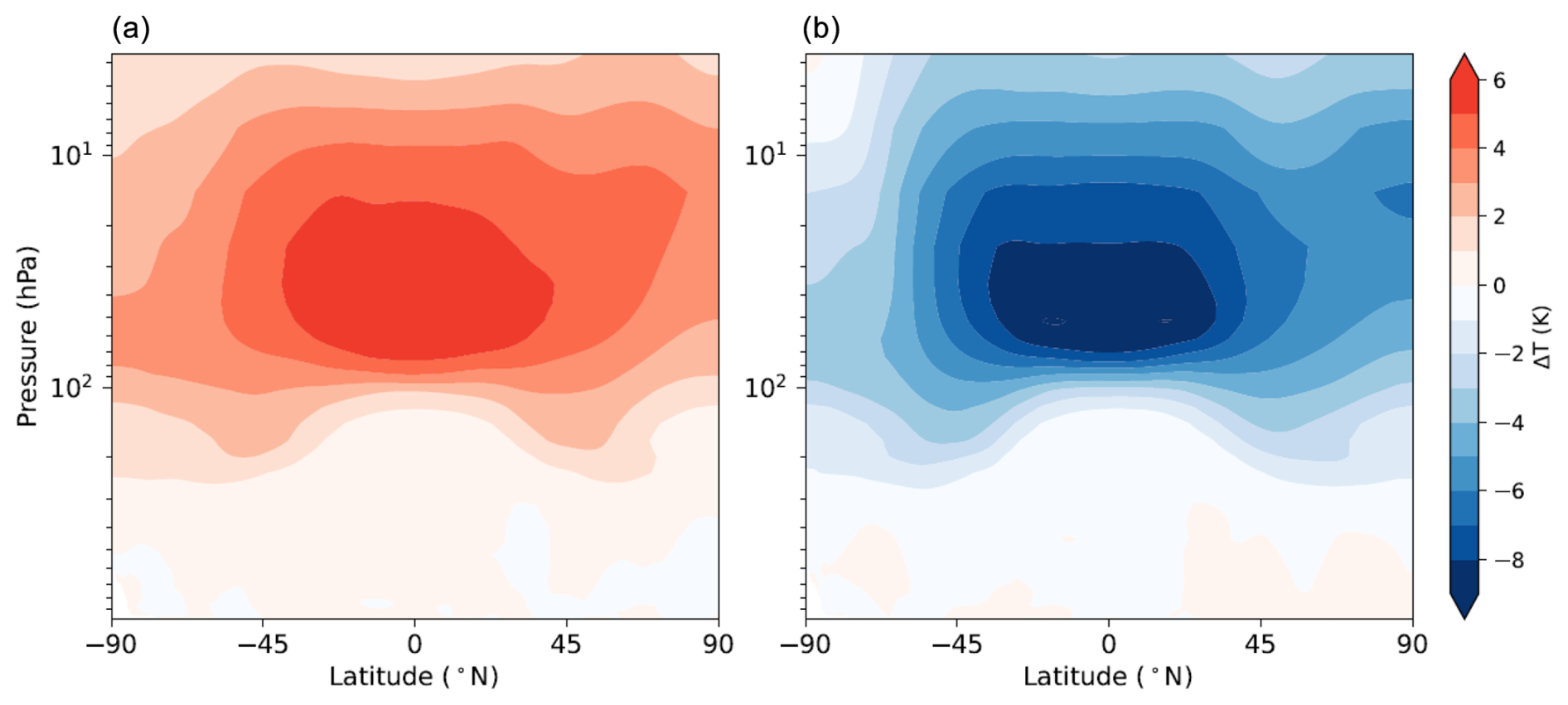
Figure 2 Zonal-mean difference in atmospheric temperature between the control integration of “Strat O₃x1.5” and the control integration of the “standard” 4xCO₂ ERF simulation (a) and between the control integration of “Strat O₃x0.5” and the control integration of the standard 4xCO₂ ERF simulation (b). Note that, for display purposes, model output on hybrid-sigma levels has been interpolated onto global-mean NorESM2-MM pressure levels.

4 Stratospheric O₃ experiments

4.1 Impact on stratospheric temperature

O₃ plays an important role in driving the thermal structure of the stratosphere due to its strong absorption of ultraviolet radiation and its absorption and emission of thermal infrared (TIR) radiation. Figure 2a shows the effect of a 50 % increase in stratospheric O₃ concentration on the zonal-mean atmospheric temperature in the control integration of NorESM2-MM. A strong increase in stratospheric temperature is evident, consistent with enhanced absorption of solar radiation and, hence, enhanced solar heating rates. The peak increase in temperature occurs in the lower stratosphere centred across the equatorial region, co-located with high insolation. Here, the maximum ΔT reaches 5.8 K. Similarly, decreasing stratospheric O₃ concentration by 50 % results in reduced absorption of solar radiation, reduced solar heating rates and a strong cooling of the stratosphere (Fig. 2b). As above, the peak temperature decrease occurs in the lower stratosphere across the Equator, with a maximum ΔT of −9 K. The impact of reduced stratospheric O₃ also propagates into the troposphere (primarily between 70 and 90° N/S), due to more downward solar irradiance reaching the lower levels of the atmosphere where enhanced absorption and heating can take place. Considering the high correlation between the 4xCO₂ IRF and 10 hPa air temperature reported by He et al. (2023), we note that at this level in particular ΔT largely increases by ≥ 3 K in the “Strat O₃x1.5” case (Fig. 2c) and largely decreases by ≥ 4 K in the “Strat O₃x0.5” case (Fig. 2b).

4.2 Impact on 4xCO₂ ERF and components

Figure 3 compares ERF, IRF and the individual adjustments for the standard 4xCO₂, Strat O₃x1.5 and Strat O₃x0.5 experiments. As shown, increasing stratospheric O₃ by 50 % has a negligible impact on the magnitude of 4xCO₂ ERF in NorESM2-MM, resulting in a near-identical forcing (of 8.47 W m⁻²) compared to the standard case (dark-orange bar). Similarly, the effect of decreasing stratospheric O₃ by 50 % has a marginal effect on 4xCO₂ ERF, increasing the forcing by just 0.23 W m⁻² relative to the standard case. Evidently, increasing or decreasing the O₃ concentration to modify stratospheric temperature (Fig. 2) does not result in a marked impact on ERF. In all three cases, NorESM2-MM simulates a considerably larger ERF than the 17 CMIP6 multi-model mean of 7.98 W m⁻² reported by Smith et al. (2020a).

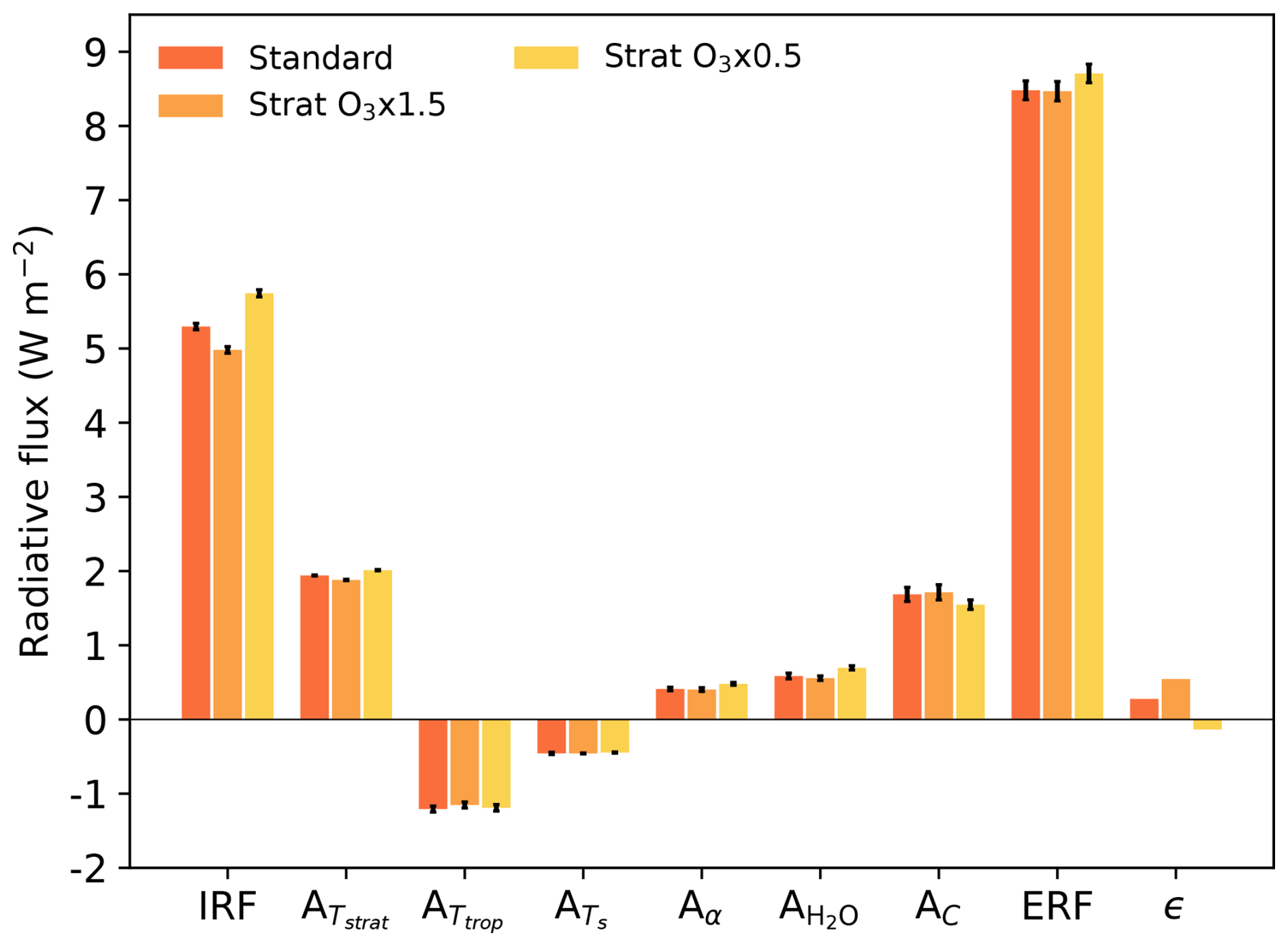
Figure 3 Comparison of NorESM2-MM “standard” 4xCO₂ ERF, IRF, adjustments and the residual term against the ERF, IRF, adjustments and the residual term diagnosed from the “Strat O₃x1.5” and “Strat O₃x0.5” experiments. All adjustments are derived using the CESM-CAM5 kernels, and all components are calculated from the average of years 6–15 of NorESM2-MM output; hence, the values for the standard 4xCO₂ case shown here differ slightly from those shown in Fig. 1. Error bars show the standard error of the mean of each component; note that we do not compute an error estimate for ϵ.

Analysis of $A_{T_{\text{Strat}}}$ further demonstrates that these experiments do not cause a significant effect on the magnitude of the temperature adjustment throughout the stratosphere, producing just a 3 % decrease and 4 % increase in this component for Strat O₃x1.5 and Strat O₃x0.5, respectively. This corroborates experiments from He et al. (2023; see their Fig. S6) that compare the size of the stratospheric temperature adjustment after a quadrupling of CO₂ from two different base states; the multi-model ensemble-mean difference in their adjustment is just −0.03 W m⁻² (although the model range is considerably larger at around 0.5 W m⁻²). As described by Shine and Myhre (2020), the magnitude of stratospheric temperature adjustment is driven by the balance between enhanced stratospheric emittance at the TOA and enhanced stratospheric absorptance of upwelling irradiance from the troposphere, which lead to a cooling and warming of the stratosphere, respectively. Following an increase in CO₂, enhanced TOA emission is greater than enhanced stratospheric absorptance because upwelling irradiance largely emanates from the cold upper troposphere with a low effective emitting temperature (e.g. Ramaswamy et al., 2001). Subsequently, the stratosphere cools, leading to a decrease in longwave emission to space, which, in turn, strengthens the TOA forcing. Given that the magnitude of $A_{T_{\text{Strat}}}$ shows little variation in Fig. 3, we can infer that the net effect of increased emissivity vs. increased absorptance is similar across each experiment, ultimately leading to a cooler stratosphere and a stronger TOA radiative imbalance in all cases. Whilst increased or decreased stratospheric O₃ affects the degree of spectral overlap with CO₂ (discussed further below) and the vertical profile of stratospheric absorption and emission, it is apparent that the base state of the stratosphere is not a significant factor in determining the magnitude of our 4xCO₂ temperature adjustments.

Evidently, the largest impact occurs on the IRF, which increases by 8 % and decreases by 6 % when stratospheric O₃ is reduced and enhanced, respectively, relative to the standard experiment. The IRF across all three experiments ranges from 4.98 to 5.74 W m⁻², resulting in a spread of around 0.8 W m⁻². This is smaller than the spread of 2 W m⁻² (ranging from around 5 to 7 W m⁻²) reported by He et al. (2023) for offline “double-call” experiments of 4xCO₂ IRF calculated with a single radiative transfer code and base states from the Atmospheric Model Intercomparison Project (AMIP) for 12 CMIP5 and CMIP6 models (hence, their spread is due only to differences in base state). However, we find closer agreement between our IRF sensitivity to 10 hPa base-state temperature and He et al. (2023), who found a near −0.1 W m⁻² K⁻¹ relation between the spread in offline double-call experiments and air temperature at this level (Fig. 1c in He et al., 2023). From Fig. 2, it can be inferred that this matches very well with the ∼ ≥ 7 K difference in StratO₃x1.5 and StratO₃x0.5 10 hPa base-state temperature and the corresponding 0.8 W m⁻² spread in IRF.

The effect on IRF can be explained principally by the impact of the O₃ concentration changes on base-state stratospheric temperature and secondarily by the spectral overlap of CO₂ and O₃.¹ In the Strat O₃x0.5 case for example, the reduced O₃ concentration induces a colder base-state stratosphere, which reduces the emission of outgoing TIR irradiance at the TOA and makes the radiative impact of a 4xCO₂ perturbation more potent. The reverse is true in the Strat O₃x1.5 case. In relation to spectral overlap, O₃ itself possesses two fundamental absorption bands in the TIR at around 9.6 and 14.27 µm, with a relatively strong band formed by overtone and combination transitions centred at 4.75 µm. As stratospheric O₃ concentrations increase, TIR absorption at these wavelengths also increases to an extent that depends on the level of band saturation and the abundance of other gases absorbing at these wavelengths. The opposite occurs if stratospheric O₃ concentrations decrease. For CO₂, the main TIR bands lie in the window regions of the H₂O spectrum, with absorption centred at 4.3 and 15 µm (the latter of which is highly significant due to its proximity to the peak of blackbody distribution for the Earth's effective emitting temperature). Weaker bands also occur near 10 µm. Regions of spectral overlap between O₃ and CO₂ therefore arise at several wavelengths: at 15 µm, the strength of CO₂ absorption largely masks the radiative effect of O₃ at 14.27 µm, and absorption by both gases at 4.75 and 4.3 µm has little impact given their location further away from the peak of Earth's blackbody distribution. However, a decreased stratospheric O₃ concentration leads to weakened absorption at 9.6 µm that allows for enhanced absorption by CO₂ at 10 µm. Likewise, increasing the stratospheric O₃ concentration results in strengthened 9.6 µm absorption that mutes CO₂. Combining the effect of base-state stratospheric temperature and spectral overlap, a 4xCO₂ perturbation therefore results in an enhancement of IRF in the Strat O₃x0.5 case relative to the standard experiment. Correspondingly, an increase in stratospheric O₃ has an opposite (albeit evidently weaker) effect.

As successive adjustments to the 4xCO₂ perturbation either strengthen or weaken IRF, the radiative impact of both O₃ experiments is either enhanced or reduced according to the sign and magnitude of each A_x term in Fig. 3 (see also Table S2 in the Supplement). Although somewhat minorly, $A_{T_{\text{Strat}}}$, $A_{T_{\mathrm{S}}}$, A_α and $A_{{\mathrm{H}}_{\mathrm{2}}\mathrm{O}}$ (as well as $A_{T_{\text{Trop}}}$ for Strat O₃x0.5) work to strengthen the difference of each experiment relative to the standard case (i.e. enhancing the TOA radiative impact for Strat O₃x0.5 and decreasing the TOA radiative impact for Strat O₃x1.5). Conversely, A_c and $A_{T_{\text{Trop}}}$ (the latter only for Strat O₃x1.5) exhibit the opposite effect, whereby the TOA radiative impact for Strat O₃x0.5 is reduced relative to the standard case and enhanced for Strat O₃x1.5.

A closer inspection of A_c (Fig. S2a in the Supplement) reveals that a significant part of this offsetting behaviour stems from ΔCRE. This is more positive for Strat O₃x1.5 (compared to the standard) and negative for Strat O₃x0.5, implying that the presence of clouds reduces the 4xCO₂ ERF in the latter. Interestingly, this phenomenon occurs due to a decidedly stronger clear-sky shortwave ERF (Table S3 in the Supplement), which reduces the difference between all-sky and clear-sky forcing (Fig. S2b), thereby resulting in a net negative ΔCRE when combined with the longwave ΔCRE (Fig. S2c and a). In general, in all cases, the 4xCO₂ perturbation induces a similar zonal-mean decrease in low-cloud fraction and increase in high-cloud fraction (Fig. S3a in the Supplement). However, relative to the standard base state, both O₃ experiments clearly have the greatest impact on cloud fraction in the upper troposphere at almost all latitudes, whereby coverage decreases in Strat O₃x1.5 and increases in Strat O₃x0.5 (Fig. S3b). As expected for high clouds, this change appears to have the strongest influence on thermal fluxes, resulting in a weaker and stronger masking of the longwave IRF for Strat O₃x1.5 and Strat O₃x0.5, respectively (Table S3). However, for the net IRF and adjustment terms (Fig. S2a), the effect of cloud masking shows little variation between each experiment and, therefore, plays a less significant role in driving the differences observed in A_c.

Finally, we note that the residual term, ϵ, also exhibits offsetting behaviour and works to counterbalance the initial radiative impact of each O₃ experiment the most (Fig. 3, Table S2), implying that non-linearity in Eq. (1) is largely responsible for dampening the differences with regard to the IRF. Overall, in each experiment, the summation of IRF, A_x and ϵ results in strikingly similar ERF values for the standard and Strat O₃x1.5 cases and a slightly larger ERF for Strat O₃x0.5.

In discussion of the potential climate implications of their findings, He et al. (2023) suggested that O₃ depletion since the 1970s could have led to a strengthening of the TOA CO₂ IRF due to the cooling of the lower stratosphere associated with O₃ loss. They theorised that the combined effect of O₃ depletion and CO₂ increase should produce a larger CO₂ ERF and a greater surface warming than model experiments that impose these perturbations separately. They calculated the indirect surface warming effect of O₃ loss by differencing surface temperature anomalies between two such sets of experiments (historical forcing between 1985 and 2014 vs. the sum of all historical forcings between 1985 and 2014 imposed independently) and inferred that the sign and spatial distribution of the non-linear warming contribution of O₃ loss to CO₂ IRF is consistent with the base-state dependence of IRF. As shown above, we demonstrate that a highly idealised reduction in stratospheric O₃ does lead to an enhancement of 4xCO₂ IRF. However, we find that this does not significantly affect the magnitude of ERF.

5 Conclusions

Here, we demonstrate that accurate calculation of IRF requires the use of host-model radiative transfer calculations, which can be computed either offline or online using double-call simulations. As noted elsewhere (e.g.  Chung and Soden, 2015b), we encourage modelling centres to make this diagnostic available with their simulations. Inferring IRF indirectly as the residual of ERF and the sum of adjustments can result in the erroneous estimation of its magnitude, which introduces further uncertainty into the exact nature of the inter-model spread in CO₂ ERF. We further show that increasing or decreasing stratospheric O₃ by 50 % results in a strong warming or cooling of the stratosphere, with the peak change in temperature in each experiment reaching around 6 or −9 K, respectively. Despite the sizeable effect on stratospheric temperature, these highly idealised changes in O₃ concentration do not result in a correspondingly large spread in the magnitude of stratospheric temperature adjustment or 4xCO₂ ERF. Instead, these experiments demonstrate a dominant impact on the magnitude of IRF, primarily due to the impact on base-state stratospheric temperature with an ancillary effect from the spectral overlap of CO₂ and O₃. Given that such large changes in stratospheric O₃ do not yield a significant impact on 4xCO₂ ERF, our results suggests that inter-model differences in stratospheric O₃ concentration are not predominantly responsible for the inter-model spread in CO₂ forcing.