Technical note: Phase space depiction of cloud condensation nuclei activation and cloud droplet diffusional growth

A novel way to represent cloud condensation nuclei (CCN) activation and cloud droplet growth by the diffusion of water vapor is introduced. The key is to apply a phase space diagram that plots the radius of a liquid droplet (deliquesced CCN or cloud droplet) versus the difference between the ambient supersaturation and the equilibrium supersaturation corresponding to the droplet radius. The latter combines the droplet and environmental characteristics, and it determines whether a droplet grows or evaporates. The diagram can be used to depict (in a straightforward way) key microphysical processes of CCN activation and deactivation as well as haze or cloud droplet transition from growth to evaporation. To show its utility, the diagram is applied to an idealized simulation of CCN activation and cloud droplet growth inside a rising turbulent air parcel and to simulations of microphysical processes inside a laboratory apparatus, the Pi cloud chamber. The adiabatic parcel mimics microphysical processes near the base of a natural cumulus or stratocumulus cloud. The Pi chamber simulations represent microphysical transformations in moist turbulent Rayleigh–Bénard convection with CCN proceeding through cycles of activation, growth, evaporation, and deactivation. A more general version of the phase diagram that is independent of the CCN dry radius is also developed. The phase diagram allows simple interpretations of key microphysical processes and highlights differences between droplet formation in natural and laboratory clouds.

1 Introduction

The formation and growth of cloud droplets are key processes with respect to understanding the properties of warm, ice-free clouds. Recent developments in numerical cloud modeling, especially the growing interest in the Lagrangian particle-based microphysics (e.g., Shima et al., 2009; Arabas and Shima, 2013; Arabas et al., 2015; Grabowski et al., 2019, and references therein; Dziekan et al., 2021; Hoffmann and Feingold, 2021; Chandrakar et al., 2022; Yang et al., 2023; Morrison et al., 2024) inspired us to revisit the problem of cloud droplets' formation and their diffusional growth in the early stages of cloud development. The narrative below provides a textbook introduction to the problem, but we feel it is appropriate to revisit elementary concepts before moving to a specific tool that we introduce in this paper.

Atmospheric cloud droplets form by a heterogeneous nucleation of microscopic aerosol particles that serve as catalysts facilitating droplet formation. Those soluble aerosols are referred to as cloud condensation nuclei (CCN). Without CCN, it is impossible to form a water droplet directly from water vapor in the Earth's natural clouds (see Wyslouzil and Wölk, 2016, for a review of theoretical and experimental studies of homogeneous water droplet formation). The equilibrium water vapor pressure over a spherical droplet containing a soluble material is described by the Köhler equation.¹ It was formulated close to a century ago by a Swedish meteorologist Hilding Köhler (Köhler, 1936). The equation incorporates two factors: (1) an increase in the saturation vapor pressure related to the surface tension of a curved droplet surface and (2) a reduction in the saturation pressure because of the dissolved CCN. The resulting form of the Köhler curve is shown in Fig. 1 and, in its simplest form, is given by the following equation:

$$\begin{array}{}\text{(1)}& S_{\text{eq}}={\displaystyle \frac{A\left(T\right)}{r}}-{\displaystyle \frac{\mathit{\kappa }{r}_{\mathrm{d}}^{\mathrm{3}}}{r^{\mathrm{3}}}},\end{array}$$

where S_eq is the equilibrium supersaturation over a spherical droplet with radius r, r_d is the CCN dry radius that describes the amount of solute inside the droplet, κ is the hygroscopicity parameter, and A is a coefficient that weakly depends on the temperature (A(273 K)=0.0012 µm). Here, we use a notation introduced by Petters and Kreidenweis (2007) that allows for characterization of CCN by a single parameter κ. However, numerical simulations discussed in this article include a more general formulation of the droplet growth equation that includes kinetic, solute, and surface tension effects (see Grabowski et al., 2011; Eqs. 2, 3, 10, and 11 therein).

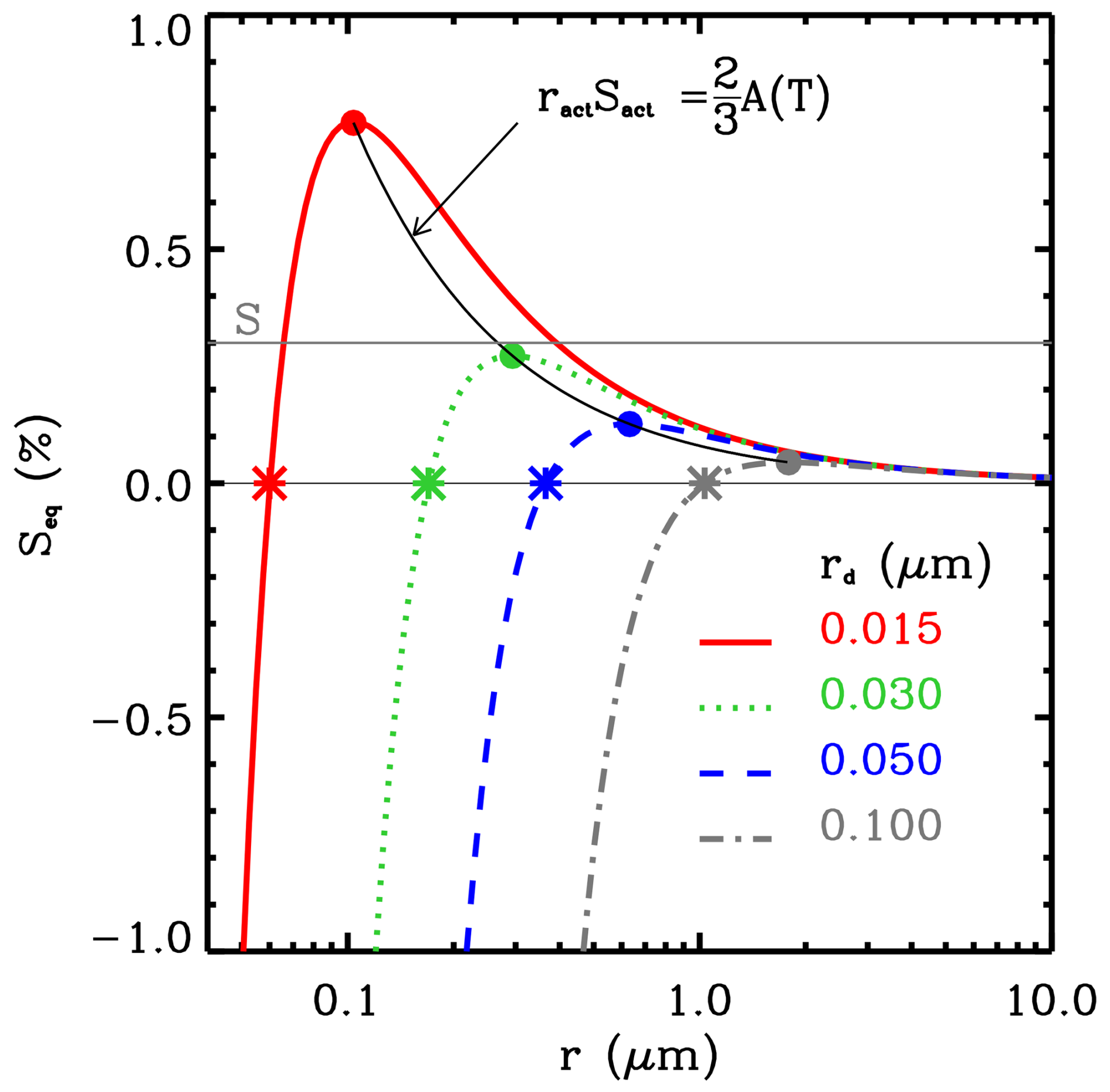
Figure 1 Examples of Köhler curves for selected dry radii of NaCl (κ=1.28) and a temperature of 273.16 K. Critical supersaturations and critical radii are marked as large dots. Radii corresponding to S_eq=0 are marked as large stars. See the text for a discussion.

Köhler curves (shown in Fig. 1) feature maxima that define the so-called critical or activation parameters: the activation radius (r_act) and the activation supersaturation (S_act). Exact values of these parameters depend weakly on the temperature, on the hygroscopicity parameter ($r_{\text{act}}\propto \sqrt{\mathit{\kappa }}$, $S_{\text{act}}\propto \mathrm{1}/\sqrt{\mathit{\kappa }}$), and on the dry CCN radius ($r_{\text{act}}\propto r_{\mathrm{d}}^{\mathrm{3}/\mathrm{2}}$, $S_{\text{act}}\propto r_{\mathrm{d}}^{-\mathrm{3}/\mathrm{2}}$). Moreover, it follows from Eq. (1) that the critical radius and critical supersaturation are inversely proportional to each other because $r_{\text{act}}{S}_{\text{act}}=\mathrm{2}/\mathrm{3}A\left(T\right)$, as shown in the figure. For the formation and early growth of cloud droplets, the most important feature of the Köhler curve is its dependence on the dry CCN radius. The peak of the Köhler curve divides nonactivated haze droplets (r<r_act) from the activated cloud droplets (r>r_act). The growth rate of the haze and cloud droplet radius squared is proportional to S−S_eq:

$$\begin{array}{}\text{(2)}& {\displaystyle \frac{\mathrm{d}{r}^{\mathrm{2}}}{\mathrm{d}t}}=a(S-S_{\text{eq}}),\end{array}$$

where a is the temperature-dependent coefficient that includes kinetic effects (e.g., Mordy, 1959; Grabowski et al., 2011). Stars in Fig. 1 mark droplet radii smaller than the critical radii that correspond to the zero equilibrium supersaturation, S_eq=0. For a given dry CCN radius, the S_eq=0 radius is equal to the critical radius divided by the square root of 3. Radii corresponding to S_eq=0 represent equilibrium haze droplet radii in the saturated environment, i.e., when S=0 or relative humidity (RH) = 100 %. It follows that haze droplets outside clouds (i.e., when RH<100 %) have smaller radii than the S_eq=0 radius. Another important feature of the Köhler curve is that the equilibrium supersaturation converges to zero (i.e., to the conditions over a plane pure water surface) for sufficiently large droplets (i.e., with radii larger than about 10 µm).

For a constant S smaller than the activation supersaturation (i.e., S for r_d=15 nm in Fig. 1), haze droplets are in a stable equilibrium. This is because a change in the environmental supersaturation (i.e., increase or decrease in S) leads to an adjustment of the haze droplet radius (increase or decrease, respectively) towards the new equilibrium size. Haze droplets formed on small, dry CCN respond rapidly to the change in the environmental supersaturation. In contrast, haze droplets formed on large CCN lag behind changes in the environmental supersaturation. This can be shown by considering the timescale characterizing droplet growth that can be taken as r over $\mathrm{d}r/\mathrm{d}t$. Neglecting the impact of the equilibrium supersaturation S_eq in Eq. (2), the droplet growth timescale is proportional to r² (see the derivation in Mordy, 1959, who considers the impact of S_eq on the droplet growth timescale). Chuang et al. (1997) puts the droplet growth timescale in the context of the timescale characterizing the environmental supersaturation change as, for instance, in the rising adiabatic parcel. Such considerations are further refined in Nenes et al. (2001), who discusses timescale limitations that may or may not lead to the eventual activation of a given CCN as well as a possible deactivation of already activated cloud droplets. Cloud droplets are in an unstable equilibrium with the environmental supersaturation S; i.e., they continue to grow away from r_act as long as S>S_eq or evaporate towards r_act when S<S_eq. In the latter case, they may deactivate (i.e., their radius may become smaller that the critical radius) and continue evaporating until S=S_eq.

Supersaturated conditions leading to cloud droplet formation can originate from two different processes: (i) uniform cooling of an air parcel (e.g., by radiative processes or by parcel expansion) or (ii) mixing of two undersaturated air parcels with different thermodynamic conditions. Both of these situations will be considered in this paper. For convective clouds, the first mechanism involves adiabatic expansion of the air parcel carried by the sub-cloud updraft towards the cloud base. A common approach to study the cloud-base CCN activation in natural clouds is to consider adiabatic parcel rising through the cloud base (e.g., Pruppacher and Klett, 1997; Reutter et al., 2009; Ghan et al., 2011). The second mechanism comes from the curvature of the saturated water vapor pressure temperature dependence. As a result, isobaric mixing of two undersaturated air parcels can lead to supersaturated conditions. This mechanism is used in the laboratory cloud chamber at the Michigan Technological University, referred to as the Pi chamber (e.g., Chang et al., 2016; Chandrakar et al., 2016; see http://phy.sites.mtu.edu/cloudchamber/, last access: 19 May 2025). Airflow inside the Pi chamber is driven by the temperature and humidity differences between 1 m apart horizontal lower and upper boundaries. Those differences drive moist turbulent Rayleigh–Bénard convection within the chamber. The supersaturation inside the chamber comes from the isobaric turbulent mixing of moist warm air rising from near the lower boundary with colder air descending from near the upper boundary.

Once air becomes supersaturated, CCN activation and formation of cloud droplets takes place. First cloud droplets form on the largest CCN because their critical supersaturation is the lowest (see Fig. 1). However, large CCN typically lag the environmental relative humidity increase, and their activation may take place after the activation of smaller CCN. The largest CCN (with dry radii larger than 1 µm, referred to as giant CCN) may never reach their critical radius, but they behave like regular clouds. With the further supersaturation increase, smaller CCN can become activated and additional cloud droplets can form. With a sufficiently large number of growing cloud droplets, the supersaturation starts to decrease because of the cloud droplets' condensational growth and the temperature increase due to latent heating. With the supersaturation decrease, it is possible that some already activated droplets can start evaporating and become deactivated (e.g., Nenes et al., 2001; Arabas and Shima, 2017; Grabowski and Pawlowska, 2023). The smallest CCN have no chance to become cloud droplets because their critical supersaturation is too high to be reached in natural clouds. They remain as haze droplets throughout the cloud life cycle. It follows that details of the CCN distribution (the total CCN concentration and concentration as a function of the dry CCN radius) as well as the environmental conditions (primarily the cooling rate, although also the air temperature) determine the partitioning between those CCN that become cloud droplets and those that remain as haze droplets. Supersaturation fluctuations due to small-scale turbulence can also impact CCN activation (e.g., Prabhakaran et al., 2020) and the partitioning between haze and cloud droplets above the cloud base (Grabowski et al., 2022a, b).

This article presents a novel way to represent CCN activation and droplet growth that can be used to depict cloud-base activation in natural clouds and microphysical processes within the Pi chamber. The key is to apply a phase space diagram that is introduced in the next section. The diagram can be used to show the instantaneous partitioning of the cloud condensate into nonactivated (haze) and activated droplets, and – perhaps more interestingly – it can be used to show the phase space trajectories of CCN activation and deactivation, as well as haze droplet or cloud droplet transition from growth to evaporation. The diagram is applied in Sects. 3 and 4 to a simulation of CCN activation and initial droplet growth inside an adiabatic parcel filled with isotropic homogeneous turbulence, as discussed in Grabowski et al. (2022b), and to simulations of droplet formation and growth in the Pi chamber, as examined in Grabowski et al. (2024). A version of the diagram that is independent of the dry CCN radius is introduced in Sect. 5. A brief summary in Sect. 6 concludes the paper.

2 The phase space diagram

Figure 2 shows the diagram that depicts key elements of CCN activation and droplet growth by the diffusion of water vapor. On the diagram, the radius of the droplet is plotted as a function of the difference between the local supersaturation S and the Köhler theory droplet equilibrium supersaturation S_eq. Because the equilibrium supersaturation S_eq depends on the droplet radius and physicochemical properties of the dissolved CCN, the horizontal axis of the diagram combines the environmental conditions with the properties of a haze droplet or cloud droplet. As the droplet diffusional growth rate is proportional to the S and S_eq difference, the solid vertical line at $S-S_{\text{eq}}=\mathrm{0}$ separates droplets that grow when the difference is positive (the right half of the diagram) from those that evaporate (on the left half) because of the negative S−S_eq difference. For small cloud droplets, the positive equilibrium supersaturation S_eq can allow their evaporation even if the ambient supersaturation is positive (e.g., Arabas and Shima, 2017; Abade et al., 2018; Grabowski and Pawlowska, 2023). For droplets with a radius larger than several micrometers, S_eq is close to zero and the S−S_eq difference is close to the ambient supersaturation S. The solid horizontal line shows the activation (critical) droplet radius that separates activated CCN (i.e., cloud droplets) above the line from haze droplets (i.e., deliquesced CCN) below the line. Except for the different symbols and switched vertical and horizontal axes, the diagram in Fig. 2 is similar to that used in Arabas and Shima (2017; see their Fig. 1). However, as shown later in the paper, we focus on more general aspects of the CCN activation and droplet growth than Arabas and Shima (2017).

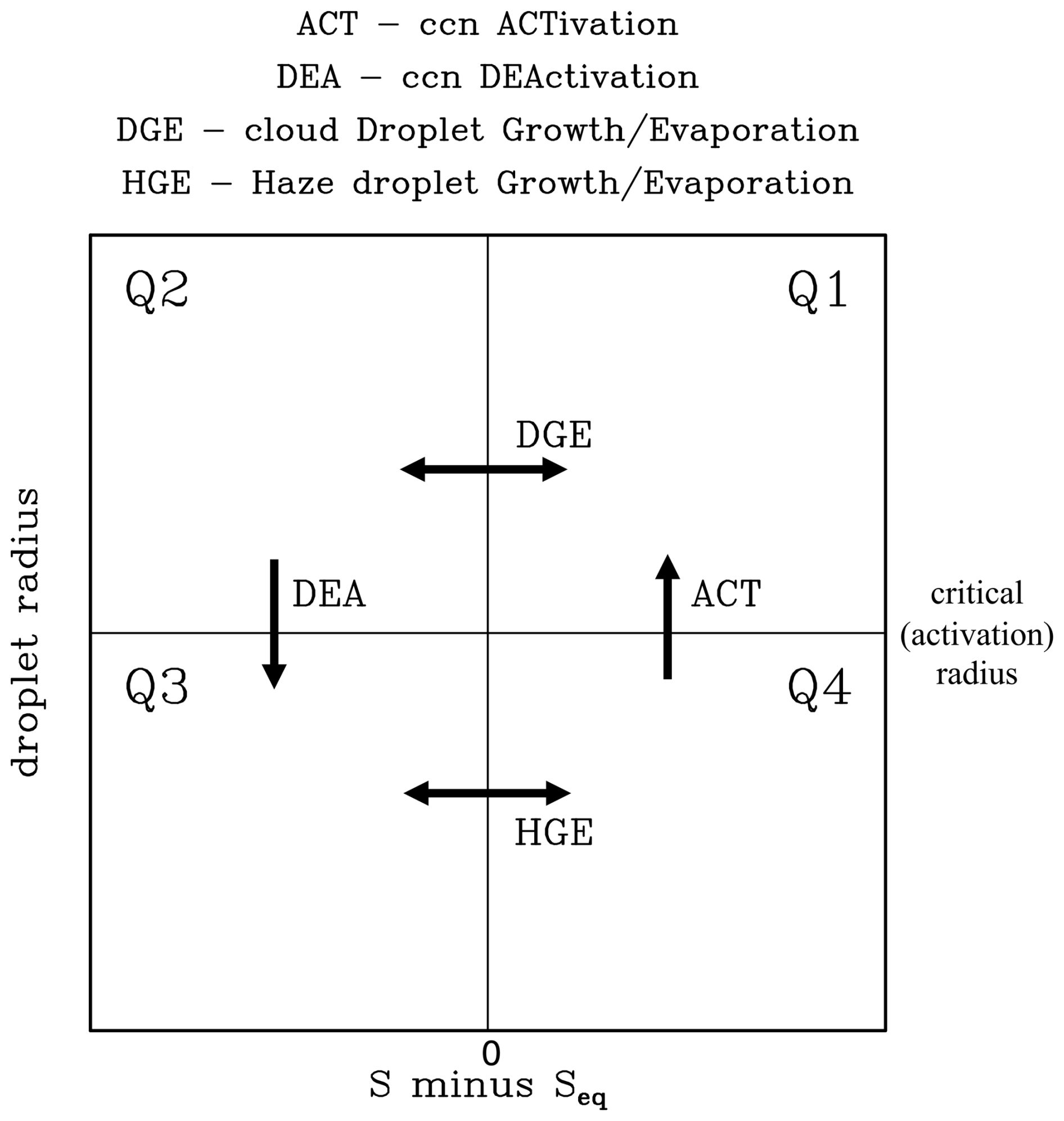
Figure 2 The phase space diagram of CCN activation and droplet growth. The solid horizontal and vertical lines show the critical (activation) radius and the zero of the S and S_eq difference, respectively. The two lines divide the phase space into four quarters, Q1 to Q4, as marked in the figure. ACT, DGE, DEA, and HGE – defined above the panel – represent haze and cloud droplet transitions during growth and evaporation. See the text for details.

The two solid lines divide the diagram into four quarters, Q1 to Q4, as marked in Fig. 2. The upper-right quarter Q1 includes droplets with a radius larger than the critical radius that feature positive S−S_eq (i.e., growing cloud droplets). The upper-left quarter Q2 contains droplets larger than the critical radius and negative S−S_eq (i.e., evaporating cloud droplets). The lower two quarters include haze droplets that either grow towards the critical radius in the right quarter Q4 or evaporate in the left quarter Q3. The arrows across the solid lines in Fig. 2 represent processes that take place during CCN activation, droplet growth and evaporation, and CCN deactivation. The activation (ACT) brings a deliquesced CCN (i.e., a haze droplet) across the critical radius line for a positive S−S_eq (i.e., from Q4 to Q1), whereas deactivation (DEA) brings an evaporating droplet across the same line in the left part of the diagram (i.e., from Q2 to Q3). ACT and DEA are one-way processes; i.e., ACT and DEA only take place in the directions shown by the arrows. Horizontal transitions represent a change from a droplet growing to evaporating or evaporating to growing in the upper part of the diagram (marked as DGE, Droplet Growth/Evaporation) and a change from a haze droplet evaporating to growing or growing to evaporating in the lower part; the latter is marked as HGE (Haze droplet Growth/Evaporation). In contrast to one-way ACT and DEA transitions, DGE and HGE can work both ways (i.e., from left to right or from right to left depending on the S−S_eq).

The next two sections discuss application of the phase diagram to CCN activation and droplet growth within an adiabatic parcel filled with turbulence rising across the cloud base (Grabowski et al., 2022b) and to microphysical processes within the simulated Pi chamber (Grabowski et al., 2024). The two sections document the advantages of using the phase diagram to investigate microphysical processes already discussed in those previous studies. In addition, the analysis further documents key differences between the two environments that have already been discussed in Grabowski et al. (2024) and provides new insights into microphysical processes in the simulated Pi chamber.

3 Application to CCN activation and droplet growth within a turbulent adiabatic parcel

Grabowski et al. (2022b; GTK22 hereafter) discuss the impact of turbulence on CCN activation within an adiabatic parcel rising across the cloud base. Activation within a nonturbulent parcel, a traditional methodology to study CCN activation at the cloud base, provides a reference. To include the effects of turbulence on CCN activation, Grabowski et al. (2022a, b) introduced a computational framework of a rising triply periodic computational domain carrying deliquesced CCN. Lagrangian particle-based microphysics (Shima et al., 2009) is applied to represent deliquesced CCN and activated cloud droplets. The turbulent parcel rises across the cloud base with a prescribed mean ascent rate that provides a spatially uniform adiabatic cooling within the parcel. Turbulent vertical velocity fluctuations provide small-scale inhomogeneities in the adiabatic cooling. The mean ascent and turbulent fluctuations lead to CCN activation within the parcel. The turbulence is assumed to be isotropic and homogeneous, and it is forced to maintain the assumed level of the turbulent kinetic energy within the parcel. The simulations apply a 64³ m³ computational domain and a 1 m grid length. The domain is filled with a weak-intensity turbulence (eddy dissipation rate of 10 cm² s⁻³ and root-mean-square turbulent velocity of about 0.2 m s⁻¹) that is arguably appropriate for the cloud-base turbulence of natural clouds (e.g., Siebert et al., 2006; Borque et al., 2016).

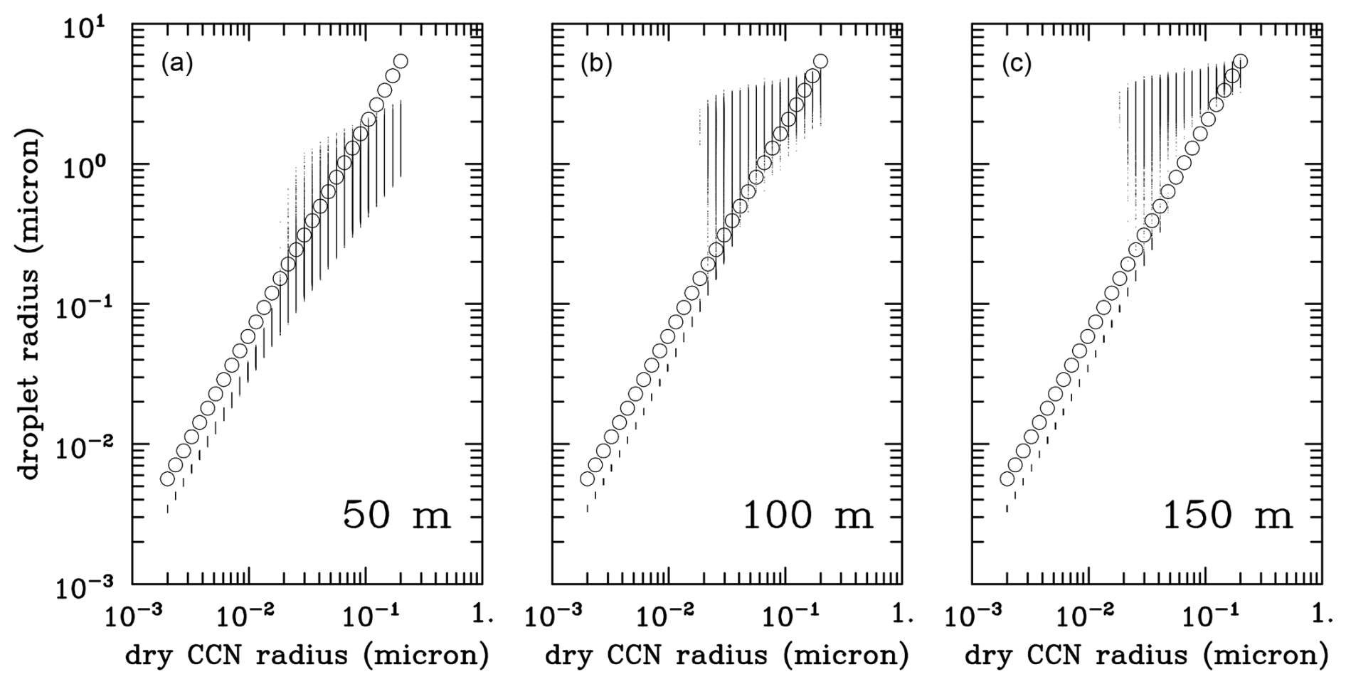
Figure 3 Scatterplot of the droplet radius versus dry CCN radius at height of 50, 100, and 150 m (panels a, b, and c, respectively) for the polluted simulation with a 1 m s⁻¹ ascent rate from GTK22. Circles represent the critical (activation) radius for each CCN bin. Of the ∼ 7.5 million droplets used in the simulation, only 5 % are shown.

The initial conditions within the domain feature a uniform 97 % RH across the volume with deliquesced CCN at equilibrium with the ambient conditions. The 200 m parcel ascent across the cloud base leads to CCN activation followed by the growth of activated cloud droplets. The CCN spectrum is based on field observations and contrasts cloud droplet formation in either pristine or polluted CCN conditions. Overall, for larger mean ascent rates, a smaller dry CCN radius separates activated and nonactivated CCN. As a result, for parcels with and without turbulence, the cloud droplet concentration is higher for a parcel rising faster across the cloud base. The key difference between nonturbulent and turbulent activation is a blurriness of the separation between dry CCN sizes featuring activated and nonactivated (haze) CCN for the turbulent case, especially for weak mean ascent rates. The blurriness comes from small-scale supersaturation fluctuations that allow CCN activation and deactivation, instead of a sharp separation between cloud and haze droplets with no turbulence-driven supersaturation fluctuations. This leads to significantly larger spectral widths in turbulent parcel simulations compared to the nonturbulent parcel when activation is completed. The blurred transition from nonactivated to activated CCN leads to the CCN activation fraction (i.e., the ratio between activated and total CCN for a given dry CCN radius) gradually increasing from zero for those CCN radii that never get activated to unity for those CCN radii that all get activated (see Fig. 10 in GTK22).

We use one of the GTK22 simulations to show how turbulent cloud-base activation is represented in the diagram introduced in the previous section. Figure 3 shows scatterplots of the droplet radius versus the dry CCN radius at three heights of the rising parcel – 50, 100, and 150 m – for a simulation with a polluted CCN distribution (total CCN concentration of 2000 cm⁻³) and mean parcel ascent rate of 1 m s⁻¹. A parcel height of 50 m is about the level at which the mean RH within the parcel reaches saturation. However, because of turbulent supersaturation fluctuations (with the standard deviation reaching close to 0.5 %; see Fig. 7 in GTK22), there are already some activated cloud droplets, as shown in Fig. 3a. At 100 m (Fig. 3b), the number of activated droplets is larger because there are more points above the critical radius. The parcel height of 100 m is about 20 m above the level of the maximum mean cloud base supersaturation of about a couple of tenths of 1 % (see Fig. 7 in GTK22). Some of the largest CCN are still not activated despite having very low critical supersaturation. This is because those large CCN grow slowly and lag ambient RH in contrast to small CCN that respond rapidly to RH changes prior to activation, as discussed in Sect. 1. At 150 m (Fig. 3c), activated droplets continue to grow, small CCN remain as haze droplets, and only some of the largest dry CCN are still smaller than the critical radius.

Figure 4 uses the phase diagram introduced in the previous section to show droplets at a 50, 100, and 150 m parcel height for two dry CCN radii, 30 and 100 nm. The results are for the turbulent parcel with a 1 m s⁻¹ mean ascent rate (as in Fig. 3). For the nonturbulent parcel, all 30 and 100 nm CCN get activated. For the turbulent parcel, all 100 nm CCN get activated (as shown in Fig. 4f). For 30 nm dry CCN within a turbulent parcel, about 82 % get activated, while about 18 % remain nonactivated at 150 m parcel height. About one-third of those nonactivated, 6 % of the total, become activated and subsequently deactivated in the fluctuating supersaturation field. Figure 4a–c show gradual CCN activation and separation between activated and nonactivated 30 nm CCN. Figure 4d–f show a gradual approach of 100 nm CCN towards activation and the subsequent growth of cloud droplets.

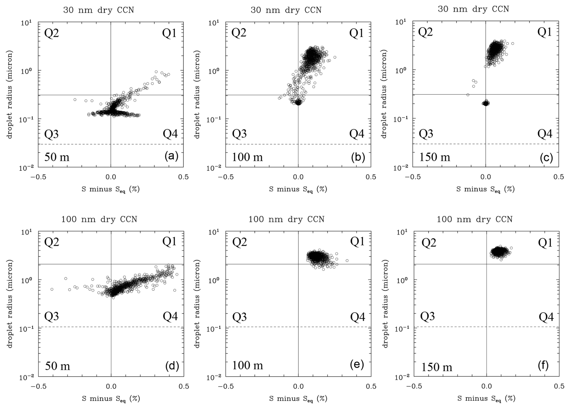
Figure 4 The phase space diagram of CCN activation and droplet growth within an adiabatic turbulence-filled parcel rising across the cloud base with a mean ascent rate of 1 m s⁻¹. The dashed horizontal line shows the dry CCN radius. Panels (a) and (d), (b) and (e), and (c) and (f) show the parcel at 50, 100, and 150 m above the starting level, respectively. Panels (d–f) and panels (a–c) are for droplets with a dry CCN radius of 30 and 100 nm, respectively. Only about 0.3 % of droplets are shown in each panel for clarity.

Figure 4 shows droplets at a particular time during parcel rise. However, the phase diagram is designed to show the evolution of selected droplets through cycles of droplet growth and evaporation. To highlight this aspect, Fig. 5 shows the evolution of a few randomly selected droplets formed on the 30 nm CCN dry radius using the same results as in Figs. 3 and 4. The left panel of Fig. 5 shows a traditional way to document parcel rise, with the droplet radius plotted as a function of the parcel height. The colored lines show examples of the simulated droplet evolution. Black lines show the evolution of five randomly selected 30 nm dry CCN that get activated and eventually form growing cloud droplets. Red lines show examples of five CCN that activate and then deactivate after a couple of tens of meters of turbulent parcel rise. Finally, green lines show examples of CCN that stay as deliquesced (haze) droplets and never reach the critical radius. As shown in Grabowski and Pawlowska (2023), activation and subsequent deactivation can also happen for a nonturbulent adiabatic parcel, especially in weak-updraft polluted clouds.

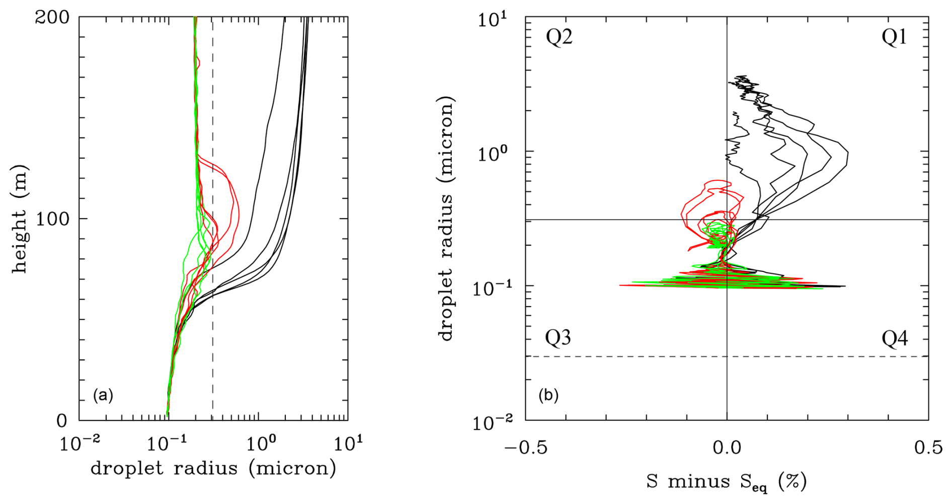
Figure 5 (a) Droplet radius as a function of height for a set of droplets from simulation as in Figs. 3 and 4 and for the dry CCN radius of 30 nm. The dashed vertical line shows the critical (activation) radius for the 30 nm dry CCN radius. Black color shows the radii of five cloud droplets that continue growing after activation. Red color represents five CCN that get activated and subsequently deactivated. Green color presents CCN that never get activated. Panel (b) shows a phase space diagram for the same droplet set as in panel (a).

Figure 5b shows the same 15 droplets on the phase space diagram applying the same colors as in Fig. 5a. The lines are not smooth because the simulation data are only saved every 2 s and because ambient conditions change rapidly in the turbulent environment. This is especially true during the early phase of the parcel rise, with deliquesced 30 nm dry CCN responding rapidly to turbulent fluctuations with haze droplet radii between 0.1 and 0.2 µm. Activated droplets (black lines) grow to a few micrometers, and the same droplets can be identified in both Fig. 5a and b. As the supersaturation decreases when the parcel moves away from the cloud base, the droplet trajectories approach the vertical line marking the zero of the S−S_eq. One of the black lines crosses the $S-S_{\text{eq}}=\mathrm{0}$ line a couple of times because of the ambient supersaturation fluctuations. This reverses the droplet growth for a short period of time, which is not easily identified in Fig. 5a. Red lines show CCN that activate and deactivate after reaching a few tenths of the 1 µm radius. Green lines show deliquesced CCN that occupy mostly quarter Q3 on the phase diagram. Both the red and green lines approach the equilibrium radius of about 0.02 µm, as seen in Fig. 5a.

4 Application to the Pi chamber simulation

Simulations from Grabowski et al. (2024; hereafter GKY24) are used to contrast activation in the adiabatic turbulent parcel from the previous section with simulated microphysical processes within the Pi chamber. Laboratory studies of moist Rayleigh–Bénard convection within the Pi chamber focus on microphysical processes of droplet formation and growth in a turbulent environment. The chamber in its cuboid configuration has an extent of 2 m×2 m in the horizontal and 1 m in the vertical. GKY24's Pi chamber simulations follow Grabowski (2020). Following the setup of one of the laboratory experiments (e.g., Thomas et al., 2019), the lower and upper boundary temperatures are 299 and 280 K, respectively, resulting in a 19 K temperature difference. The side wall temperature is assumed to be the mean of the lower- and upper-boundary temperatures at 289.5 K. The computational domain is covered with a 51³ uniform grid, and the horizontal and vertical grid lengths are 0.04 and 0.02 m, respectively. Lagrangian particle-based microphysics is used to represent the growth of haze CCN and cloud droplets that include kinetic, solute, and surface tension effects (Grabowski et al., 2011). For illustration, the phase diagram is applied to one of the simulations discussed in GKY24. The simulation, referred to as C40, applies an observationally based dry CCN distribution with two lognormal modes centered at radii of 20 and 75 nm, and the total CCN concentration is 40 cm⁻³. The simulated mean droplet concentration for the C40 case is about 30 cm⁻³ (see Fig. 3 in GKY24).

Figure 6 shows an instantaneous phase space diagram for the dry CCN of 10, 30, and 100 nm. For clarity, the figure includes only 2 % of all droplets from the last snapshots of model data, at minute 20 of the simulations. Droplets cover all four quarters, Q1 to Q4, with haze droplets and cloud droplets growing and evaporating at the time of the plot. Similar plots at different times are similar, with the pattern shown in the figure being similar across the entire computational domain.

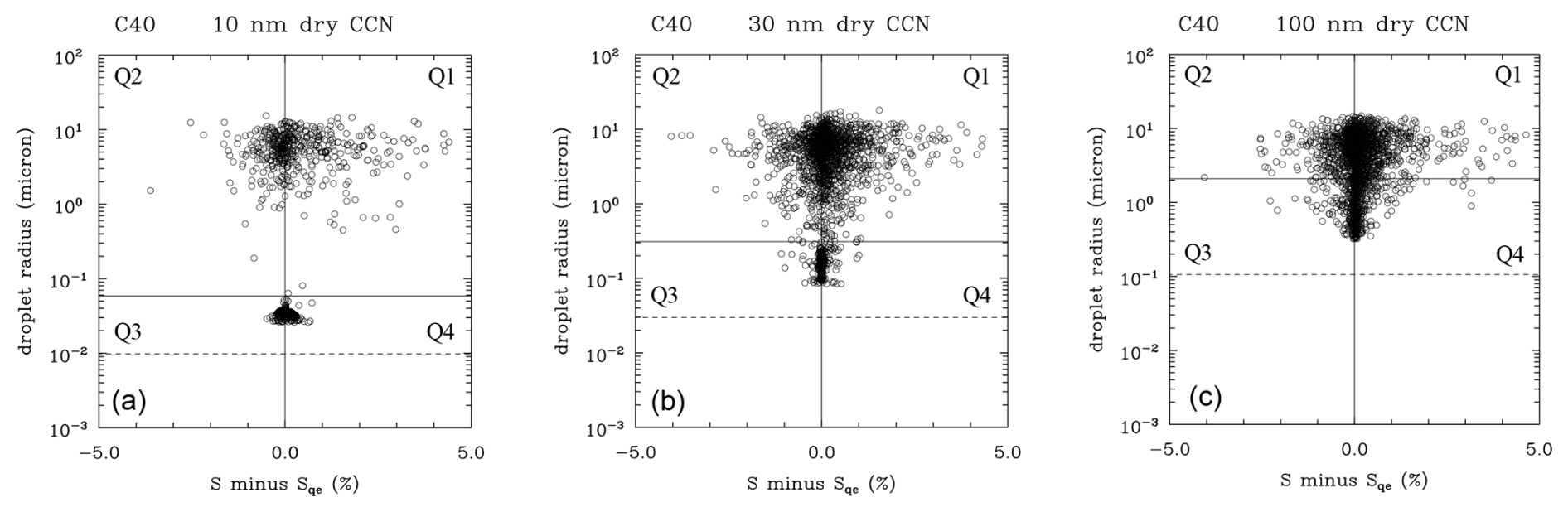
Figure 6 The instantaneous phase space diagram for minute 20 of the C40 simulation from GKY24. Panels (a), (b), and (c) are for the dry CCN radius of 10, 30, and 100 nm, respectively. The dashed line show the dry CCN radius. Only 2 % of all data points are used in each panel.

Figure 6 provides a static picture; i.e., it does not include evolution of individual droplets. To show the evolution, the C40 simulation was restarted at minute 20 and run for an additional 5 min. The evolution for droplets with a 10, 30, and 100 nm dry CCN radius was saved every half second along with the S−S_eq averaged over the preceding half second. The latter is because the droplet radius change from one half second to another comes from the S−S_eq averaged over the half second. The idea is to show how individual droplets within the Pi chamber progress through their cycles of deliquescence, activation, growth, evaporation, and deactivation while they move within the chamber carried by the chamber-scale flow. Figure 7 shows an example of model results for three randomly selected 10 nm dry CCN radius droplets. Figure 7a, c, and e show the evolution of the droplet vertical position within the 1 m deep chamber, and Fig. 7b, d, and f show the associated droplet trajectories on the phase diagram. The line color in Fig. 7a, c, and e shows the quarter in Fig. 7b, d, and f in which the droplet is located at a given moment in time. Colors and corresponding quarters are shown above the left panels. Q1, Q2, Q3, and Q4 refer to the upper-right, upper-left, lower-left, and lower-right quarters, respectively, as in Fig. 2. The plots are for three randomly selected droplets out of about 125 000 droplets with a 10 nm CCN dry radius. As expected, the left panels show that droplets circulate up and down inside the chamber. However, as already mentioned in GKY24, the vertical droplet motion has little to do with droplet growth because the supersaturation comes from the turbulent mixing inside the chamber, not from the vertical air motion and adiabatic cooling as in natural clouds.

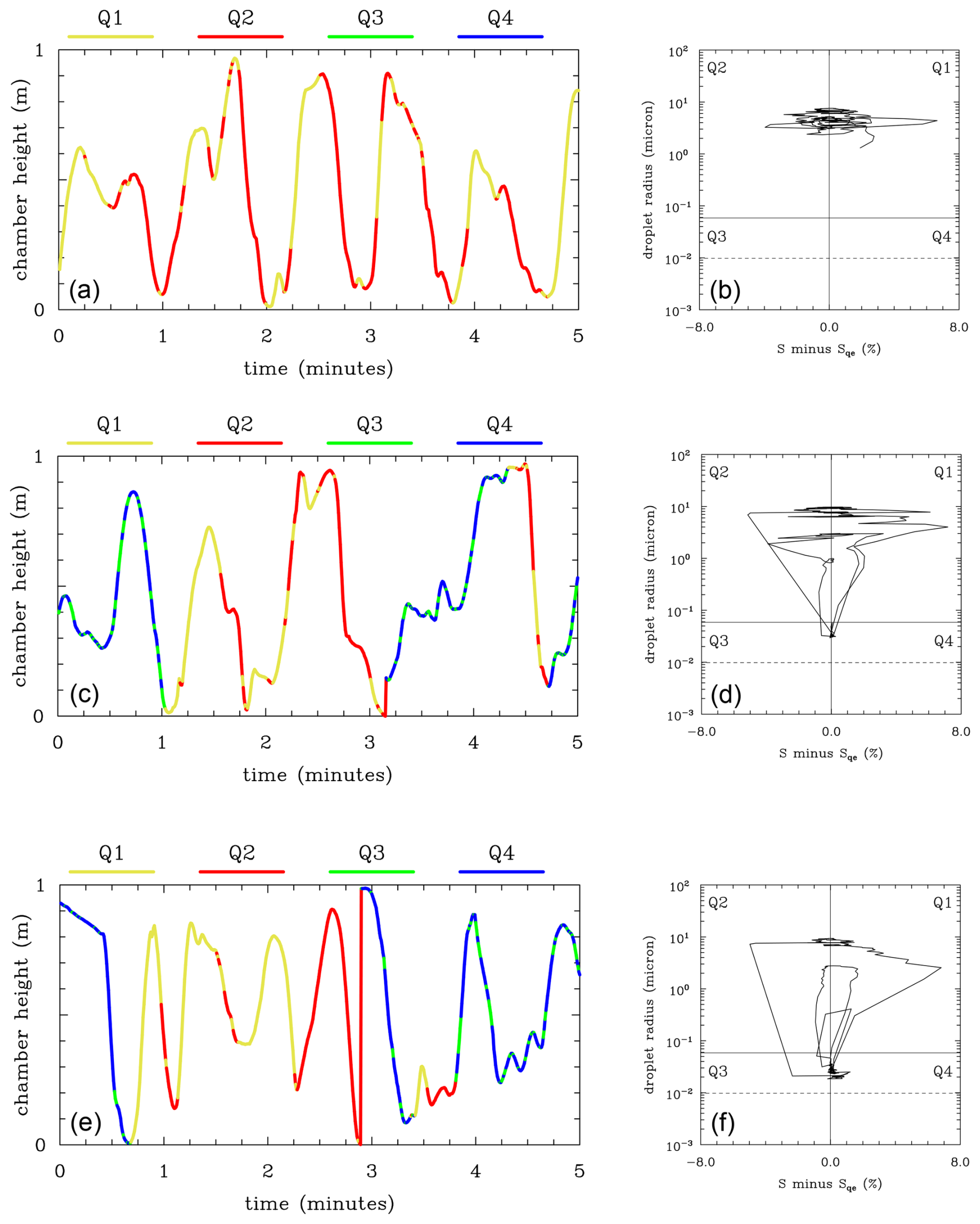
Figure 7 Results for C40 simulations from GKY24 for a 10 nm dry CCN radius. (a, c, e) Evolution of the droplet height in the Pi chamber for three randomly selected droplets, with colors marking the droplet position on the phase space diagram. Colors defining the quarters on the diagram (Q1 to Q4) are shown above each left panel. (b, d, f) Representation of droplet trajectories on the phase diagram.

As the panels in Fig. 7 show, two out of the three droplets go through cycles of droplet activation and deactivation (i.e., crossing the horizontal solid line) as well as growing and evaporating as haze droplets and cloud droplets (i.e., deliquesced CCN with a radius smaller and larger than the critical radius, respectively). The droplet depicted in the top row of Fig. 7 remains activated over the 5 min period (i.e., it remains above the solid line in Fig. 7b, d, and f, and its space trajectory only includes red and yellow colors).

One can count the time that all 10 nm dry CCN radius droplets spend in each quarter of the diagram. The results are as follows: about 28 % of the time is spent in Q1 (activated cloud droplets that grow), about 24 % of the time is spent in Q2 (activated cloud droplets that evaporate), about 13 % of the time is spent in Q3 (evaporating haze droplets), and about 35 % of the time is spent in Q4 (growing haze droplets). The partitioning between activated droplets (Q1 and Q2) and haze droplets (Q3 and Q4) approximately agrees with Fig. 9 in GKY24, which shows an activation fraction of about 50 % for the CCN with a 10 nm dry radius. The same statistics for 30 and 100 nm dry CCN show slightly higher numbers for Q1 and Q2 (consistent with an activation fraction close to 60 % for those CCN, as shown in Fig. 9 of GKY24) and corresponding reductions in Q3 and Q4 (not shown). The lowest number for all three CCN is for Q3: 13 %, 14 %, and 20 % for a 10, 30, and 100 nm dry radius, respectively.

One can calculate transfer statistics between various quarters as shown in Fig. 2. Table 1 presents the average number of transfers per droplet during the 5 min simulation for haze and cloud droplets formed on 10, 30, and 100 nm dry CCN in the C40 simulation. The statistics are for activation (ACT), deactivation (DEA), and transfers from growth to evaporation for cloud droplets (DGE) and haze droplets (HGE). Transfers for growth and evaporation for cloud droplets (between Q1 and Q2) and haze droplets (between Q3 and Q4) are separated into those from left to right (i.e., evaporation into growth), marked with a “+” sign, and those from right to left (i.e., growth into evaporation), marked with a “−” sign. As the table shows, the transfer statistics are similar for the three dry CCN radii. The differences do not seem statistically significant considering the standard deviations among all droplets (shown in parentheses). The activation and deactivation numbers are small considering other transfer numbers in the table. This seems to agree with the results shown in Fig. 7, which documents frequent transfers between Q1 and Q2 as well as between Q3 and Q4, with smaller numbers of Q4 to Q1 and Q2 to Q3 transfers (i.e., ACT and DEA). The haze droplet transfers (HGE) are the most frequent, and their number decreases with the dry CCN increase. The latter is likely because of an increased “inertia” of large CCN that follow ambient supersaturation fluctuations with more difficulty than small CCN.

Table 1 Averaged number of transfers per dry CCN defined in Fig. 2 for cloud and haze droplets formed on 10, 30, and 100 nm dry CCN radii during the 5 min of the additional simulation. Two-way transfers (DGE and HGE) are separated into those from left to right (+) and those from right to left (−). The numbers in parentheses show the standard deviation among all droplets for a given dry CCN radius.

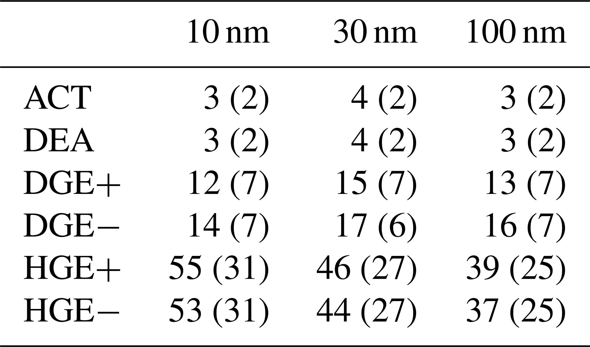
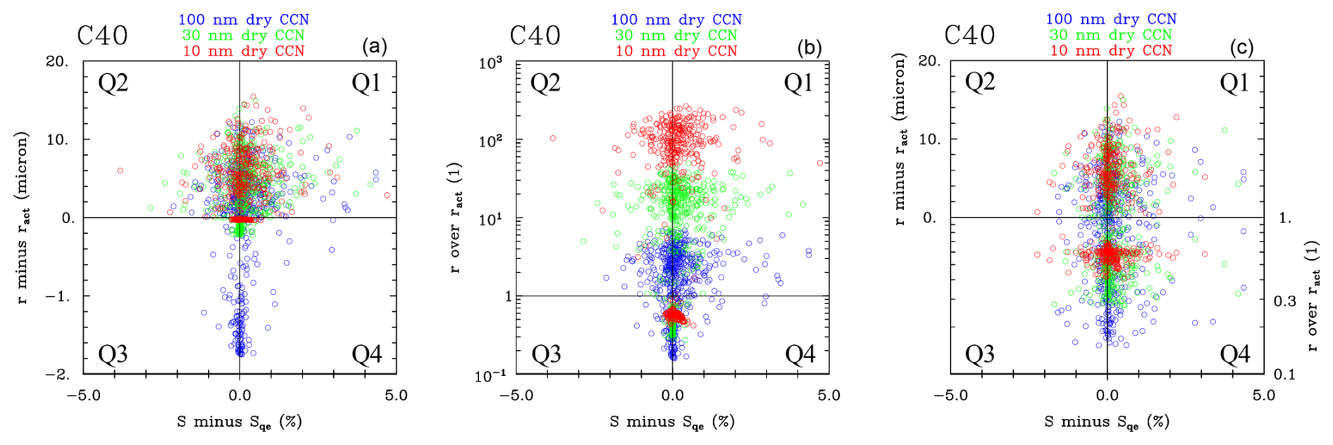
Figure 8 Results for C40 simulations from GKY24. The same data are used as in Fig. 6 but on the modified phase diagram and with a smaller number of points (0.5 % for each dry CCN radius). Red, green, and blue colors represent droplets formed on CCN with a 10, 30, and 100 nm dry radius, respectively. The same data are shown in all panels. Panel (a) applies the difference between the droplet radius and critical radius on the vertical axis. Panel (b) uses the ratio between the droplet radius and the critical radius. Panel (c) applies either the difference between the droplet radius and critical radius when the difference is positive (quarters Q1 and Q2) or the ratio between the droplet radius and the critical radius in the Q3 and Q4 quarters.

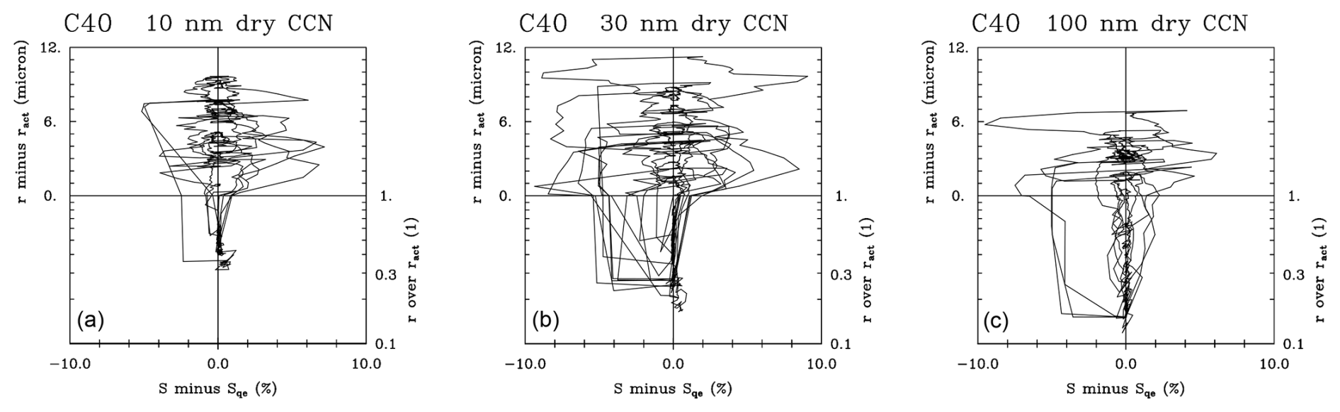
Figure 9 Representation of droplet trajectories on the generalized phase diagram for C40 simulation. Results are for three randomly selected droplets for a (a) 10 nm, (b) 30 nm, and (c) 100 nm dry CCN radius.

5 Phase space diagram independent of dry CCN radius

The diagram introduced in Sect. 2 and applied to simulations in Sects. 3 and 4 depends on a specific dry CCN radius. A more general phase diagram that can be applied to different CCN dry radii might also be of interest. One option might be to plot the difference between the droplet radius and the activation (critical) radius on the vertical axis, rather than the droplet radius. Such a modification makes the diagram independent of the dry CCN radius. However, in such a case, it is impossible to use a logarithmic scale on the vertical axis when the difference is negative for the haze droplets. The logarithmic scale is convenient because of a large radius range between haze and cloud droplets; for that reason, it was used in the figures in Sect. 3 and 4. Another option is to consider the ratio between the droplet radius and the activation (critical) radius that facilitates, in a natural way, the application of the logarithmic scale. Figure 8 shows the two options in panels a and b for droplets formed on three dry CCN radii, 10 nm (red color), 30 nm (green color) and 100 nm (blue color), from the C40 simulation discussed in the previous section (e.g., Fig. 7). As shown in Fig. 8a, the linear scale for the difference between the droplet radius and the critical radius is good for cloud droplets in the upper half of the diagram because they all have similar radius ranges. However, such a choice is poor for haze droplets because the critical radius varies between 60 nm for the 10 nm dry CCN radius and about 2 µm for the 100 nm dry CCN radius. In contrast, as shown in Fig. 8b, using the ratio between the droplet radius and the critical radius better fits the haze droplets, but then cloud droplets are separated, as the ratio between the droplet radius and the critical radius varies over 2 orders of magnitude. A sensible compromise is to use the difference between the droplet radius and the activation (critical) radius for cloud droplets and the ratio between the droplet radius and the critical radius for the haze droplets. Such an approach, shown in Fig. 8c, combines quarters Q1 and Q2 from Fig. 8a and quarters Q3 and Q4 from Fig. 8b.

Figure 9 shows the evolution of several droplets using the generalized phase space diagram from Fig. 8c. Figure 9a–c show the evolution of droplet trajectories from additional 5 min C40 simulations for three droplets formed on a 10, 30, and 100 nm dry CCN radius, respectively. (The three droplets for 10 nm dry CCN have already been used in Fig. 7.) The generalized phase space diagram allows a direct comparison of droplet trajectories that is independent of the CCN dry radius. Figure 9 shows that larger dry CCN feature smaller r and r_act ratios for haze droplets. Moreover, the results in Fig. 9 seem to agree with those in Table 1; i.e., there are fewer trajectories passing through the activation and more passages between growth and evaporation, especially for haze droplets. However, one has to keep in mind that Fig. 9 only shows nine randomly selected droplets (three for each dry CCN radius), whereas Table 1 includes statistics for all droplets.

6 Summary

This paper introduces a phase space diagram that documents, in a simple way, microphysical processes leading to cloud droplet formation and growth. The diagram shown in Fig. 2 plots the haze or cloud droplet radius versus the difference between ambient supersaturation S and the equilibrium supersaturation S_eq corresponding to the droplet radius. The difference combines droplet and environmental characteristics and determines whether the droplet grows or evaporates. A similar diagram was used by Arabas and Shima (2017; see their Fig. 1) to discuss CCN activation and subsequent deactivation of a droplet with a radius larger than the critical radius when the ambient supersaturation S falls below the equilibrium supersaturation S_eq (i.e., when S−S_eq becomes negative). See also relevant discussions in Nenes et al. (2001), Abade et al. (2018), and Grabowski and Pawlowska (2023). The current paper applies the diagram to depict the CCN activation, droplet growth, evaporation, and deactivation, especially relevant to microphysical processes taking place in fluctuating supersaturation due to cloud turbulence. For illustration, the diagram is applied to numerical simulations of the impact of turbulence on cloud-base CCN activation and to cycles of CCN activation and deactivation inside the Pi cloud chamber. Cloud-base activation is driven by adiabatic cooling of the rising air, with turbulence modifying the sharp separation between activated and nonactivated CCN. Cloud chamber simulations mimic microphysical transformations in the moist Rayleigh–Bénard convection that are driven by turbulent mixing between humid warm and cold air. The Pi chamber supersaturation comes from the nonlinear dependence of the saturated water vapor pressure on temperature.

The cloud-base CCN activation in fluctuating supersaturation due to cloud turbulence is discussed in Grabowski et al. (2022b). Here, we use one of the simulations to illustrate the application of the phase diagram to depict phase space trajectories of (i) CCN that form cloud droplets that continuously grow above the cloud base, (ii) CCN that activate and subsequently deactivate, and (iii) CCN that never activate. For the cloud-base activation, the partitioning between the three pathways (i)–(iii) depends on the dry CCN radius, with small CCN never becoming activated and large CCN always activating to form cloud droplets. The new diagram is also applied to the microphysical processes within the Pi chamber discussed in Grabowski et al. (2024). We use one of the Pi chamber simulations to document cycling of the CCN through activation, growth of cloud droplets, their evaporation, and CCN deactivation. The three dry CCN sizes selected from two CCN distributions considered in Grabowski et al. (2024), a dry radius of 10, 30, and 100 nm, seem to move over the phase diagram in a similar fashion to those documented in Table 1. This is in contrast to the cloud-base activation discussed in Grabowski et al. (2022b). The two cases considered in Sects. 3 and 4 (i.e., droplet formation/growth at/above the base of a natural cloud versus the cycling of droplets through activation, growth, and evaporation inside the laboratory cloud chamber) highlight differences between microphysical processes in natural and laboratory clouds.

A generalized form of the diagram is introduced in Sect. 5. The motivation is to create a diagram that is independent of the dry CCN radius. The generalized phase diagram uses the difference between the droplet radius and the activation (critical) radius for cloud droplets as well as the ratio between the two for haze droplets. A linear scale is used for cloud droplets, whereas a log scale is used for haze droplets. For illustration, the generalized diagram is applied to Pi chamber simulations to compare activation, growth, evaporation, and deactivation of various dry CCN radii.

Application of the new diagram to simulations of entrainment and mixing for cumulus or stratocumulus clouds might be especially enlightening. This is not only because of the activation of entrained CCN but also because of droplet evaporation and CCN deactivation as a result of cloud dilution. Detailed analysis of microphysical processes associated with cloud entrainment and mixing is possible when applying the new phase space representation. We plan to pursue this line of research in the near future.