Quantifying the sources of increasing stratospheric water vapour concentrations

According to satellite measurements from multiple instruments, water vapour (H₂O) concentrations, in most regions of the stratosphere, have been increasing at a statistically significant rate of ∼1 %–5 % per decade since the early 2000s. Previous studies have estimated stratospheric H₂O trends, but none have simultaneously quantified the contributions from all main sources (temperature variations in the tropical tropopause region, changes in the Brewer–Dobson circulation, and changes in methane (CH₄) concentrations and oxidation) at all latitudes. Atmospheric Chemistry Experiment–Fourier Transform Spectrometer (ACE-FTS) measurements are used to estimate altitude-/latitude-dependent stratospheric H₂O trends from 2004–2021 due to these sources. Results indicate that rising temperatures in the tropical tropopause region play a significant role in the increases, accounting for ∼1 %–4 % per decade in the tropical lower mid-stratosphere and in the mid-latitudes below ∼20 km. By regressing to ACE-FTS N₂O concentrations, it is found that, in the lower mid-stratosphere, general circulation changes have led to both significant H₂O increases and significant H₂O decreases on the order of 1 %–2 % per decade depending on the altitude/latitude region. Making use of measured and modelled CH₄ concentrations, the increase in H₂O due to CH₄ oxidation is calculated to be ∼1 %–2 % per decade above ∼30 km in the Northern Hemisphere and throughout the stratosphere in the Southern Hemisphere. After accounting for these sources, there are still regions of the mid-latitude lower mid-stratosphere that exhibit significant residual H₂O trends increasing at 1 %–2 % per decade. Results indicate that these unaccounted-for increases could potentially be explained by increases in upper-tropospheric molecular hydrogen.

1 Introduction

Water vapour (H₂O) is the most abundant greenhouse gas in the Earth's atmosphere. Much like other greenhouse gases, it absorbs shortwave radiation near the surface, leading to temperature increases, and emits longwave radiation in the stratosphere and above, leading to upper-atmospheric cooling. Near the surface, H₂O is part of a positive feedback loop where increasing temperatures lead to an increase in the saturation vapour pressure, leading to more H₂O in the atmosphere, leading to more heating, and so on. Because H₂O is controlled predominantly by this feedback system in the troposphere and because of its much shorter atmospheric lifetime (with respect to other greenhouse gases) on the order of weeks near the surface and 10–20 years in the stratosphere (Brasseur and Solomon, 2005), H₂O is typically considered an amplifier of the greenhouse effect rather than a contributor (e.g. Chung et al., 2014). Downward-propagating radiation from stratospheric H₂O can also lead to upper-tropospheric heating (e.g. Manabe and Wetherald, 1967; de F. Forster and Shine, 1999; Forster and Shine, 2002). It is therefore important to continually monitor and understand H₂O variations throughout the troposphere and stratosphere.

Although the predominant source of stratospheric H₂O is moisture-rich tropospheric air that is lofted upwards in the tropics as part of the Brewer–Dobson circulation (BDC), the physical processes that control the amount of water vapour in the stratosphere are fundamentally different from those in the troposphere. As that moisture-rich tropospheric air crosses the cold tropical tropopause region, it freeze-dries, removing most of the H₂O before entering the stratosphere (Brewer, 1949; Holton and Gettelman, 2001, and references therein). With few other sources, and its relatively long stratospheric lifetime, much of the stratospheric H₂O budget is a function of tropical tropopause cold-point temperature, especially in the lower stratosphere. As such, time series of tropical tropopause region temperatures are often used as a regressor in determining stratospheric H₂O trends (Hegglin et al., 2014, and references therein). Hegglin et al. (2014) showed that variations in low- to mid-latitude and lower-stratospheric H₂O very closely followed variations in modelled mean tropical temperatures at 100 hPa. At higher altitudes and more poleward latitudes, H₂O variations tended to follow those of the modelled temperatures with a lag of a few months (tape recorder effect; Mote et al., 1996).

Another major source of stratospheric H₂O is methane (CH₄) oxidation via reactions with OH, O(¹D), and Cl. As detailed in Brasseur and Solomon (2005), oxidation of CH₄ via OH can produce H₂O directly, but all three reactions have byproducts that lead to the production of a formaldehyde molecule (CH₂O), which is then quickly destroyed via multiple reactions that can produce H₂O molecules. In the stratosphere, on average, an oxidized CH₄ molecule produces approximately two H₂O molecules; however, that average varies with altitude and latitude (e.g. Jones et al., 1986; le Texier et al., 1988; Frank et al., 2018).

A minor source of stratospheric H₂O is the oxidation of H₂, which can be an indirect product of CH₄ oxidation or be transported into the stratosphere from the tropical troposphere. Both Wrotny et al. (2010) and Frank et al. (2018) have shown that it is possible for the ratio of H₂O production to CH₄ loss, α, in the tropical stratosphere to be greater than 2. Wrotny et al. (2010) used satellite measurements from the Halogen Occultation Experiment (HALOE), Atmospheric Chemistry Experiment–Fourier Transform Spectrometer (ACE-FTS), and the Michelson Interferometer for Passive Atmospheric Sounding (MIPAS) to show that α can be on the order of 2.0–3.7, attributing the additional production to oxidation of H₂ that was not produced via CH₄ oxidation.

A number of studies have recently been conducted that measured stratospheric H₂O increases from satellite measurements; however, none of them parse trends in order to determine the relative contributions from each of the three main sources throughout the stratosphere. For instance, similarly to Hegglin et al. (2014) and Tao et al. (2023), Randel and Park (2019) used merged HALOE and Aura/Microwave Limb Sounder (MLS) data to show that the majority of variations in lower-stratospheric H₂O from 1993–2017 can be explained by changes in tropical cold-point temperature. Yue et al. (2019) determined that both Sounding of the Atmosphere using Broadband Emission Radiometry (SABER) and Aura/MLS measurements have exhibited stratospheric H₂O trends on the order of 5 %–6 % per decade since the early 2000s. As to the sources of those increases, they determined that the H₂O trends in the lower stratosphere are consistent with frost-point hygrometer measurements and that mesospheric trends are much greater than what is expected assuming complete CH₄ oxidation. Similarly, Fernando et al. (2020) found that profiles of global ACE-FTS, Aura/MLS, and SABER H₂O trends agreed well but that they could not be explained solely by CH₄ oxidation. ACE-FTS is in a unique position when it comes to investigating the influence of CH₄ oxidation on stratospheric H₂O trends, as it is currently the only Earth-observing satellite instrument that makes vertically resolved measurements of both H₂O and CH₄ throughout the stratosphere.

This study uses simultaneously measured profiles of H₂O, CH₄, and N₂O from ACE-FTS (a measurement combination that only ACE-FTS is currently producing) in order to measure height-resolved H₂O trends throughout the stratosphere in latitudinal bands spanning 80° S–80° N. The sources of those trends are then quantified, considering contributions due to temperature changes in the tropical tropopause region, structural changes in the BDC, and changes in CH₄ concentrations in the local and tropical tropopause region.

A description of the satellite measurements used in this study can be found in Sect. 2, and the methodology is described in Sect. 3. The ACE-FTS H₂O trends and the contributions from different sources are discussed in Sect. 4, and all the results are summarized in Sect. 5.

2 ACE-FTS on SciSat

The ACE-FTS instrument (Bernath et al., 2005) is one of two instruments on board the Canadian SciSat satellite, which was launched into a high-inclination orbit in August 2003. Starting in February 2004, the ACE-FTS instrument began measuring profiles of temperature, pressure, and concentrations of multiple atmospheric trace species, including H₂O, CH₄, and N₂O. The instrument is a high-spectral-resolution (0.02 cm⁻¹) spectrometer viewing the Earth's limb in the infrared between 750 and 4400 cm⁻¹, using solar occultation viewing geometry. The vertical profiles span 5–150 km with a vertical spacing of ∼2–6 km, depending on the orbital geometry, and the circular field of view at the tangent altitude is on the order of 3–4 km. This study makes use of the most recent version of level 2 data, version 5.2 (v5.2), which provides interpolated data on a 1 km grid. The retrieval algorithm, described by Boone et al. (2005, 2013, 2020, 2023), uses a non-linear, least-squares, global-fitting technique that fits observed atmospheric transmission spectra to forward-modelled spectra in species-/altitude-dependent microwindows. The modelled spectra are calculated using spectral line parameters from the HITRAN2020 database (Gordon et al., 2022). In all retrievals, horizontal homogeneity is assumed, and diurnal variations are not taken into account along the line of sight.

Version 5.2 of the H₂O retrievals makes use of 63 microwindows between 937 and 3173 cm⁻¹; has altitude limits of 5 and 95 km; and in the stratosphere accounts for CO₂, O₃, N₂O, CH₄, NO₂, HNO₃, NO, and COF₂, as well as isotopologues H₂O, CO₂, N₂O, and CH₄ as interfering species. ACE-FTS H₂O has been used in over 50 different studies, including the European Space Agency's Water Vapour Climate Change Initiative (Hegglin and Ye, 2022; Ye et al., 2022), merged data studies (e.g. Froidevaux et al., 2015; Davis et al., 2016), and multiple validation studies (e.g. Wetzel et al., 2013; Weaver et al., 2019; Rong et al., 2019). Fernando et al. (2020) examined ACE-FTS v4.0 H₂O and CH₄ trends in the stratosphere and mesosphere but focused on 55° S–55° N mean values. Although the study did not quantify the different sources contributing to H₂O trends, it was concluded that increasing CH₄ trends were not sufficient to fully explain the observed increases in stratospheric H₂O.

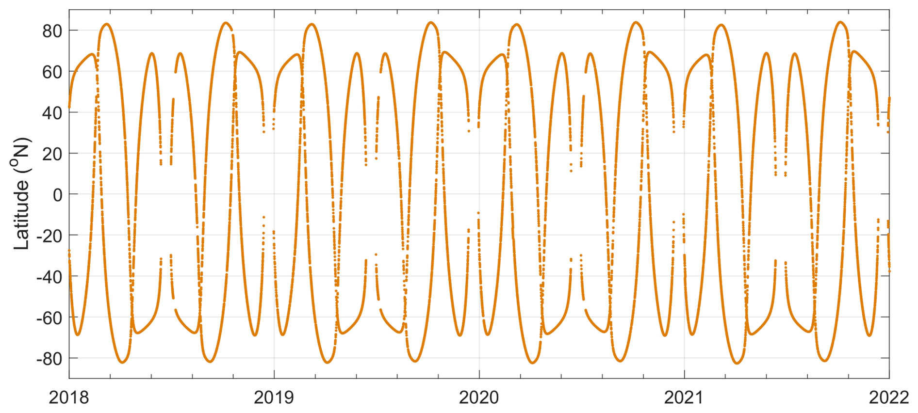
The latitudinal coverage of the instrument is shown in Fig. 1. As can be seen, the annually repeating measurements are made predominantly in the high latitudes, with the tropics being sampled roughly every 3 months. However, significant trends are still capable of being detected at the lower latitudes due to the long lifetime of the ACE-FTS data sets.

Figure 1 Latitudinal coverage of the ACE-FTS measurements for 2018–2022.

3 Methodology

Many different trends are calculated in this study, each of them making use of the multiple linear regression (MLR) technique (Chatterjee and Hadi, 1986), using various predictor data sets (in different combinations) as regressors. In each case, whether it is ACE-FTS H₂O, CH₄, or N₂O trends, the time series are fit to a model of the form

$$\begin{array}{}\text{(1)}& {\displaystyle }{\displaystyle }{y}_{\text{fit}}={\mathit{\beta }}_{\mathrm{0}}+{\mathit{\beta }}_{\mathrm{1}}l\left(t\right)+\sum _i{\mathit{\beta }}_i{r}_i\left(t\right),\end{array}$$

where t is time in years, β denotes the fit components, l(t) is a linear function increasing from −0.5 to 0.5 over the length of the time series being fitted, and r(t) denotes the considered regressor time series. The regressor time series used in this study are

• two annual oscillation terms (AO), cos 2πt and sin 2πt, and two semi-annual oscillation (SAO) terms, cos 4πt and sin 4πt, with t measured in years;

• monthly mean tropical tropopause region temperatures from the European Centre for Medium-Range Weather Forecasts (ECMWF) Reanalysis version 5 (ERA5; Hersbach et al., 2020) data (as described below);

• simultaneously measured ACE-FTS N₂O data as a proxy for dynamical processes (Dubé et al., 2023). As per Dubé et al. (2023), local N₂O time series at all altitudes and latitudes have a 2.8 % per decade trend (corresponding to the 2004–2022 global surface N₂O trend) removed prior to being used as a regressor;

• daily mean F10.7 cm solar radio flux values (which indirectly affect H₂O concentrations via influences on O₃ and temperature) provided by Geomagnetic Observatory Niemegk, Potsdam (Matzka et al., 2021);

• monthly mean Quasi-Biennial Oscillation (QBO) proxies of the 30 and 50 hPa Singapore zonal winds (Baldwin et al., 2001; obtained from https://www.geo.fu-berlin.de/en/met/ag/strat/produkte/qbo/index.html, last access: 30 September 2023);

• monthly mean El Niño–Southern Oscillation (ENSO) index values from the NOAA Physical Sciences Laboratory (Wolter and Timlin, 2011; obtained from https://psl.noaa.gov/enso/mei/, last access: 30 September 2023);

• monthly mean tropopause pressure (trop) values from NCEP-NCAR reanalysis data (Kalnay et al., 1996; obtained from https://psl.noaa.gov/data/reanalysis/reanalysis.shtml, last access: 10 January 2025).

H₂O trends were calculated at all ACE-FTS altitudes (1 km grid) between 17.5 and 55.5 km – roughly between the hygropause and stratopause – in 16 10° bins between 80° S and 80° N for daily mean time series. To avoid influences from measurements within and near the polar vortexes, scaled potential vorticity (sPV) values derived from the Modern Era Retrospective analysis for Research and Applications, Version 2 (MERRA-2; Gelaro et al., 2017) interpolated to ACE-FTS locations (Manney et al., 2007) were employed. Only data with a corresponding absolute sPV value of $\mathrm{1.4}\times {\mathrm{10}}^{-\mathrm{4}}$ s⁻¹ or less were used in this study.

In order to fit to tropical tropopause region temperatures, a time series of monthly mean temperatures within 15° S–15° N at 100 hPa for the years 1988–2022 was obtained from ERA5 data (shown in Fig. 2). In the tropical lower stratosphere, it is expected that the H₂O time series would closely follow the ERA5 temperature time series. However, at locations further from the tropical lower stratosphere, the H₂O response is expected to be lagged with respect to the temperature time series, as it takes longer for air entering the stratosphere to reach those locations, as discussed above. In the fitting algorithm, at each altitude and latitude bin, the regression was performed with the ERA5 temperatures lagged by 0–15 years in 2 d increments to find the lag time that minimized the residual between the ACE-FTS H₂O data and the MLR fit. Only lag times that led to a positive correlation between the H₂O and temperature time series were considered, and the lagged temperature time series will be referred to hereafter as T_lag. At the lowest altitude level in the 0–10° S and 0–10° N latitude bins, lag times were restricted to within 2 months, and lag times at any other given altitude/latitude bin were restricted to a value within ±24 months of adjacent bins. Although the ERA5 time series was lagged by up to 15 years in each altitude/latitude bin, it was found that the maximum lag time required to minimize the residuals in any bin was 60 months, whereas stratospheric mean age-of-air estimates tend to be on the order of 0–15 years, depending on altitude and latitude. This can be explained by the fact that lagging the temperature time series assumes that the measured air parcel is a singular parcel that travelled from the entry point to the measurement location with a particular transit time and does not account for mixing or changes in transit pathways (Poshyvailo-Strube et al., 2022).

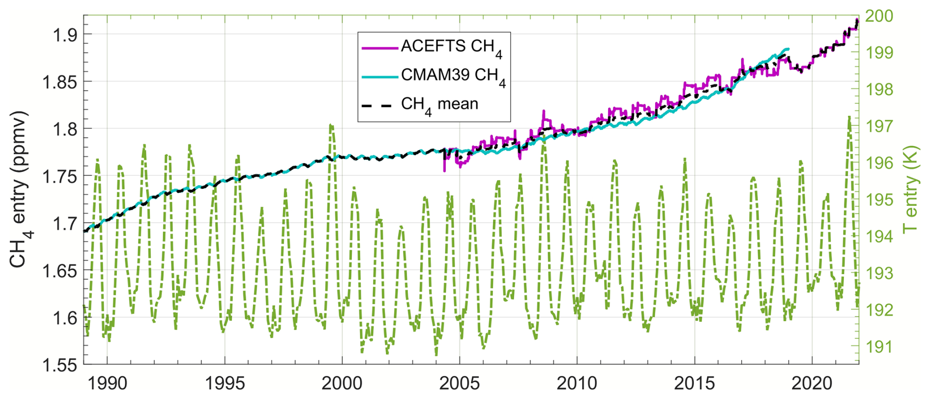
Figure 2 Mean CH₄ time series for 15° S–15° N and 100–200 hPa. ACE-FTS data (cyan) are 180 d running means, and the CMAM39 data (magenta) are daily means. The mean of ACE-FTS and CMAM39 (dashed black line) was used to determine the CH₄ entry trend. Also, ERA5 temperatures (green dot-dash line) are monthly mean values for 15° S–15° N at 100 hPa. See text for details.

To ensure that it is appropriate to simultaneously use T_lag and local N₂O time series as regressors, the correlation between these time series was calculated in each altitude and latitude bin. At all altitudes and latitudes, the absolute correlation between measured N₂O and T_lag time series is less than 0.35 and is typically below 0.2. The same is true for the correlation between N₂O and the seasonal cycles and for T_lag and SAO – although, between T_lag and SAO, the correlation is typically on the order of 0.2–0.3. T_lag and AO, however, are not independent, as the tropopause region temperatures exhibit a significant annual oscillation. The implications of this are discussed in Sect. 4.2.

Although CH₄ oxidation is a major source of stratospheric H₂O, ACE-FTS measurements of local CH₄ concentrations are not an appropriate regressor, as local H₂O concentrations depend on the amount of CH₄ that has been oxidized in the air parcel since entering the stratosphere, which is a function of the difference between the CH₄ concentration at time of entry and the local CH₄ concentration,

$$\begin{array}{ll}{\displaystyle }[{\mathrm{H}}_{\mathrm{2}}\mathrm{O}{]}_{{\mathrm{CH}}_{\mathrm{4}}}& {\displaystyle }=\mathit{\alpha }[{\mathrm{CH}}_{\mathrm{4}}{]}_{\text{oxidized}}\\ \text{(2)}& {\displaystyle }& {\displaystyle }=\mathit{\alpha }\left(\right[{\mathrm{CH}}_{\mathrm{4}}{]}_{\text{entry}}-\left[{\mathrm{CH}}_{\mathrm{4}}{]}_{\text{local}}\right),\end{array}$$

where α is the H₂O yield from oxidized CH₄. In past studies, α is often assumed to be a constant of 2 throughout the stratosphere (e.g. Stowasser et al., 1999; Myhre et al., 2007; Frank et al., 2018). However, Frank et al. (2018) showed that this assumption tends to overestimate H₂O production in the lower stratosphere and underestimate H₂O production nearer the stratopause. In this study, a height-dependent α is used based on the global effective H₂O yield profile shown in Fig. 14 of Frank et al. (2018), which is ∼1.6 in the lower stratosphere and ∼2.2 at the stratopause. To account for the fraction of H₂O trends due to CH₄ oxidation, the time derivative of Eq. (2) is taken,

$$\begin{array}{}\text{(3)}& {\displaystyle }{\displaystyle \frac{\mathrm{d}[{\mathrm{H}}_{\mathrm{2}}\mathrm{O}{]}_{{\mathrm{CH}}_{\mathrm{4}}}}{\mathrm{d}t}}=\mathit{\alpha }({\displaystyle \frac{\mathrm{d}[{\mathrm{CH}}_{\mathrm{4}}{]}_{\text{entry}}}{\mathrm{d}t}}-{\displaystyle \frac{\mathrm{d}[{\mathrm{CH}}_{\mathrm{4}}{]}_{\text{local}}}{\mathrm{d}t}}).\end{array}$$

The local CH₄ trends are determined by regressing to ACE-FTS N₂O data (in addition to AO and SAO time series) to account for changes in CH₄ due to changes in the general circulation,

$$\begin{array}{}\text{(4)}& {\displaystyle }\begin{array}{rl}& {\displaystyle \frac{\mathrm{d}[{\mathrm{CH}}_{\mathrm{4}}{]}_{\mathrm{local}}}{\mathrm{d}t}}={\mathit{\beta }}_{\mathrm{0}}+{\mathit{\beta }}_{\mathrm{1}}l\left(t\right)\\ & +\sum _i({\mathit{\beta }}_{{\mathrm{AO}}_i}{\mathrm{AO}}_i+{\mathit{\beta }}_{{\mathrm{SAO}}_i}{\mathrm{SAO}}_i)+{\mathit{\beta }}_{{\mathrm{N}}_{\mathrm{2}}\mathrm{O}}\left[{\mathrm{N}}_{\mathrm{2}}\mathrm{O}\right].\end{array}\end{array}$$

Since ACE-FTS has low sampling in the tropical region, model data from the specified dynamics run of the Canadian Middle Atmosphere Model (CMAM39-SD) (Beagley et al., 1997; Scinocca et al., 2008; McLandress et al., 2014) were used to supplement the ACE-FTS data when calculating CH₄ entry trends. The CMAM39-SD run (referred to as CMAM39 hereafter) spans 1979–2018 inclusive, with simulations relaxed towards 6-hourly fields of temperature, vorticity, and divergence from ERA-Interim (Dee et al., 2011) reanalysis data. The chemical forcing fields for long-lived greenhouse gases, including CH₄, were obtained from the Coupled Model Intercomparison Project Phase 6 (CMIP6) Eyring et al., 2016) historical time series (Meinshausen et al., 2017) up to 2014 and the SSP2-4.5 scenario (Meinshausen et al., 2020) for the remaining years. They were forced as a time-dependent mixing ratio specified for the bottom two model layers (approximately 100 m in depth) based on the global and annual average mixing ratio taken as the mid-year value and linearly interpolated in time to provide values at intermediate times.

The mean of the ACE-FTS 15° S–15° N, 100–200 hPa, 180 d running zonal mean and the CMAM39 15° S–15° N, 100–200 hPa daily zonal mean was calculated, as shown in Fig. 2. This ACE-CMAM mean time series (dashed black line in Fig. 2) was used to determine a CH₄ entry trend of 78±1 ppbv per decade between 2004 and 2022. The uncertainties for $\frac{\mathrm{d}[{\mathrm{CH}}_{\mathrm{4}}{]}_{\text{entry}}}{\mathrm{d}t}$ and $\frac{\mathrm{d}[{\mathrm{CH}}_{\mathrm{4}}{]}_{\text{local}}}{\mathrm{d}t}$ are added together in quadrature, as are the uncertainties in $\frac{\mathrm{d}[{\mathrm{H}}_{\mathrm{2}}\mathrm{O}{]}_{{\mathrm{CH}}_{\mathrm{4}}}}{\mathrm{d}t}$ and the fitted H₂O trend uncertainties (all uncertainties are the statistical uncertainties of the calculated trends, excluding measurement uncertainties, which are assumed to be negligible). This method, however, assumes that CH₄ trends at the stratospheric entry point have been constant from the time of entry to the time period for which the local CH₄ trends are being calculated, which could be a difference of up to the order of 1 decade. As seen in the CMAM CH₄ time series, and as discussed by authors such as Dlugokencky et al. (2003) and Rigby et al. (2008), there was a slowdown in the increase in CH₄ concentrations just before the beginning of the ACE mission (∼1999–2003) just below the tropical tropopause. This feature is accounted for and discussed when examining H₂O trends using time-lagged CH₄ entry trends in Sect. 4.2.

All ACE-FTS data were screened for outliers using data quality flags, as per Sheese et al. (2015), prior to analysis. At all altitude levels used in this study, the screening rejects less than 1 % of the data. Only data prior to 2022 were used, so as to avoid any influence from H₂O injected by the Hunga Tonga–Hunga Ha'apai eruption in January 2022.

4 Results

The following sections discuss results of MLR trend analysis on the ACE-FTS H₂O time series using different regressors. The “full” H₂O trends are those where only the AO and SAO time series (that do not themselves have any trend) are used as regressors. Results are also shown for H₂O “residual” trends, which are the resulting trends when using additional time series that may contain a trend as regressors. The differences between the full trends and the residual trends (labelled as Δ in figure panels) are considered to be the contribution to the full trend due to the regressors used in the analysis.

Section 4.1 discusses both the full H₂O trends and the individual contributions to the full H₂O trends due to solar flux, QBO, and ENSO influences; structural BDC changes; and changes in tropical tropopause region temperatures. Section 4.2 analyzes the contribution to the full H₂O trends due to CH₄ oxidation under two different assumptions: firstly, simply assuming a constant $\frac{\mathrm{d}[{\mathrm{CH}}_{\mathrm{4}}{]}_{\text{entry}}}{\mathrm{d}t}$ over the past few decades and then accounting for the fact that $\frac{\mathrm{d}[{\mathrm{CH}}_{\mathrm{4}}{]}_{\text{entry}}}{\mathrm{d}t}$ has not been constant and allowing the value used to vary depending on altitude and latitude. The discussion then focuses on the remaining residual trends, which can still be statistically significant, after all the above-mentioned individual sources contributing to the full trends are accounted for.

4.1 Standard MLR results

A simple MLR analysis of the ACE-FTS H₂O trends, regressing only to annual and semi-annual cycles, is shown in the left panel of Fig. 3, and the corresponding trend uncertainties (95 % confidence level) are shown in the right panel. The results clearly show that, since 2004, stratospheric H₂O has been increasing or has had no significant trend throughout the stratosphere. There is a noted hemispheric asymmetry at all altitudes, except for around the highest altitudes, ∼50–55 km, where trends are on the order of 2 %–3 % per decade. In the Southern Hemisphere (SH), H₂O trends also tend to be on the order of 2 %–3 % per decade, except near the tropical lower stratosphere. In the Northern Hemisphere (NH), H₂O trends tend to be somewhat more variable, with values of 3 %–5 % per decade up to ∼30 km and ∼1 %–3 % per decade above 30 km.

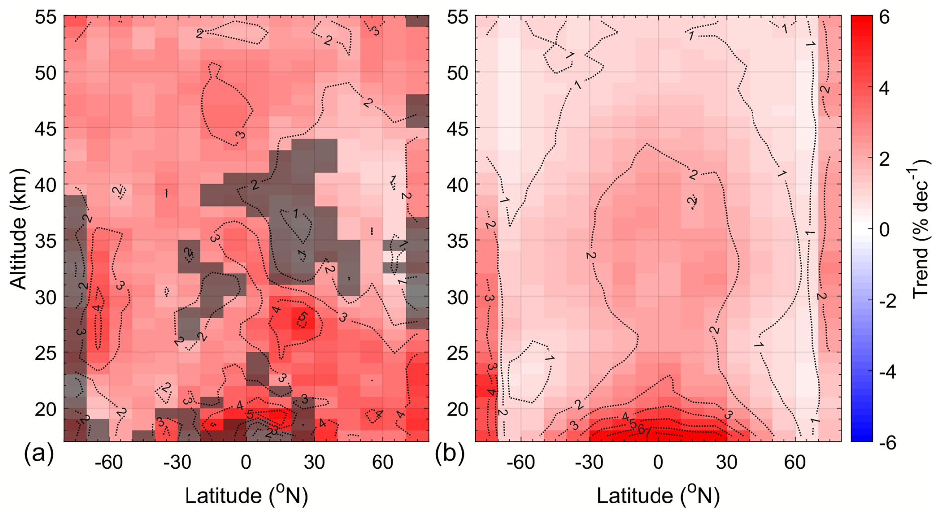
Figure 3 ACE-FTS H₂O trends. (a) Full trends (where only regressing to semi-annual and annual cycles) and (b) corresponding trend uncertainty to a confidence level of 95 %. Shaded regions in panel (a) indicate regions with no significant trend to within 95 %.

The left panel of Fig. 4 again shows the trend results from a simple MLR analysis of the ACE-FTS H₂O time series, regressing only to annual and semi-annual cycles, and these are shown to compare to the residual H₂O trends when regressing to the F10.7 cm, QBO, ENSO, and trop time series, shown in the middle panel. The differences in the H₂O trend values are typically less than ±0.5 % per decade in all altitude/latitude bins (except within 70–80° S), and the differences due to F10.7 cm alone are typically only within ±0.2 % per decade (not shown). The effects of time-lagging ENSO and trop are discussed in Appendix A1.

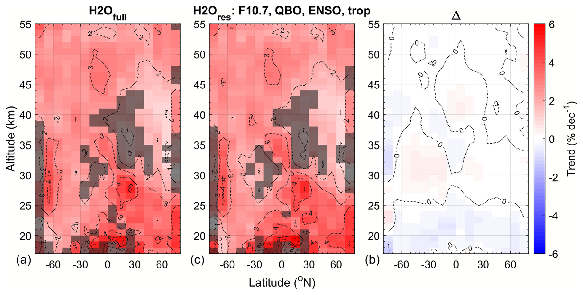
Figure 4 ACE-FTS H₂O trends. (a) Full trends (where only regressing to semi-annual and annual cycles). (b) Residual H₂O trends after regressing to F10.7 cm, QBO, ENSO, and tropopause pressure time series and semi-annual and annual cycles. (c) The difference between the full trends and the residual trends. Shaded regions in panels (a) and (b) indicate regions with no significant trend to within 95 %.

In all following analyses, QBO, ENSO, and trop indices are not used in the regression schemes, as the effects they are meant to represent can also be accounted for by the ACE-FTS N₂O time series.

As shown in Dubé et al. (2023), simultaneous measurements of N₂O, a long-lived atmospheric tracer, can be used as a proxy for changes in the BDC and can be used as an alternate regressor to account for trends due to dynamical processes in the stratosphere. The middle panel of Fig. 5 shows the residual H₂O trends after regressing to local ACE-FTS N₂O, and the right panel shows the difference between the full H₂O trend and those after regressing with N₂O. The remaining trends are all increasing (Fig. 5, middle panel), but the hemispheric asymmetry in the lower stratosphere flips sign (compared to the full trends), and the remaining trends are more strongly positive in the SH (∼3 % per decade) compared to the NH (1 %–3 % per decade). Above ∼35 km, the remaining H₂O trends are more consistent between hemispheres, on the order of 1 %–3 % per decade. These results are consistent with those of Tao et al. (2023). The differences (right panel of Fig. 5) represent the trend in H₂O due to changes in the general circulation, showing that the net hemispheric asymmetry in H₂O trends can be attributed to changes in stratospheric circulation. In particular, the influence can be to either increase or decrease local H₂O concentrations, depending on the region. Changes in the BDC account for an increase in H₂O of 1 %–2 % per decade in the NH near 20–30 km and a decrease in H₂O of 1 %–2 % per decade in the NH near 30–40 km and in the SH near 25–30 km. In all other regions, the contribution of dynamical processes to H₂O trends is not statistically significant.

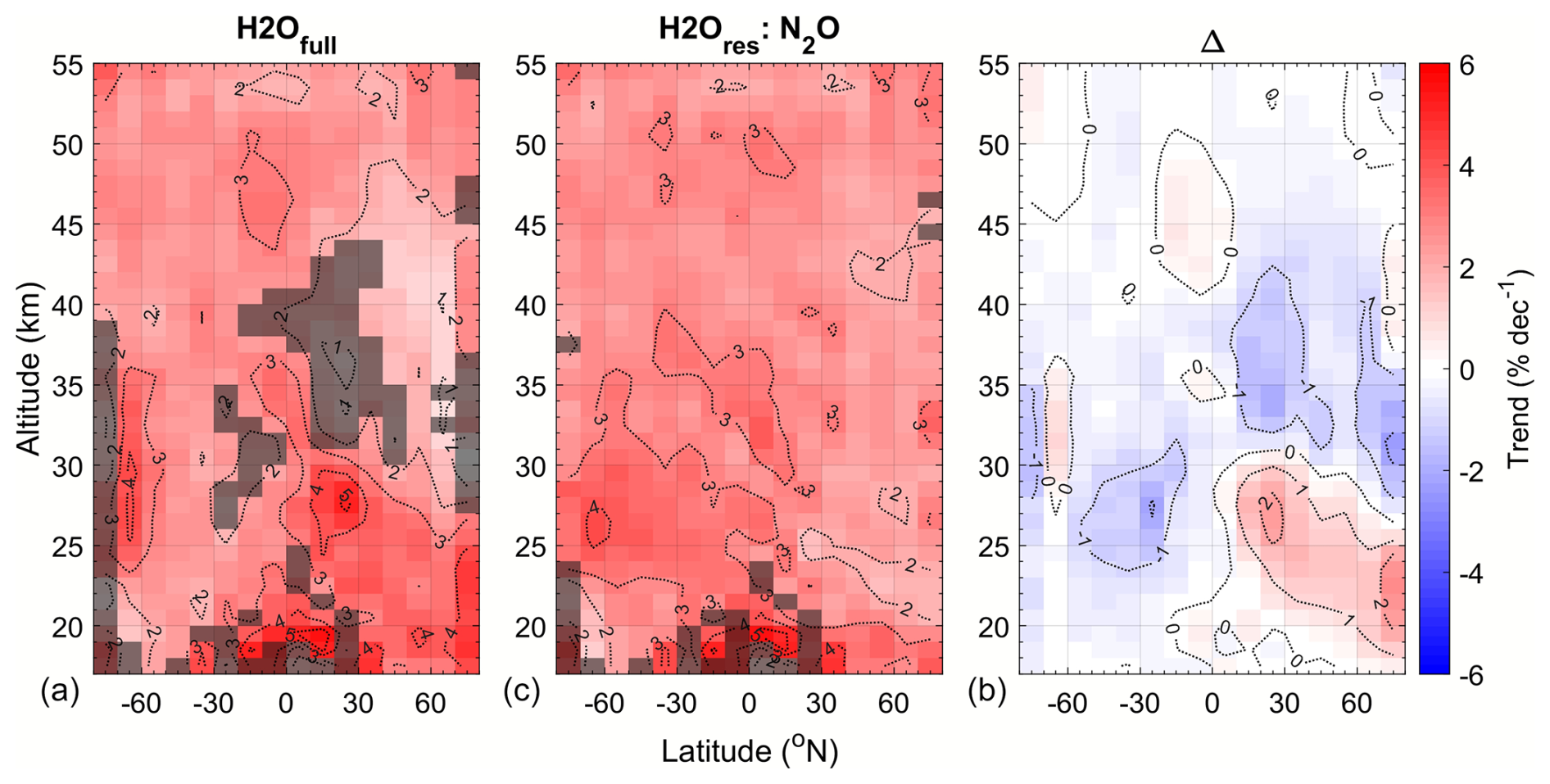
Figure 5 Same as Fig. 4, except the residual H₂O trends (b) are after regressing to N₂O and semi-annual and annual cycles.

Climate models have long indicated that increasing concentrations of greenhouse gases in the lower atmosphere should lead to an acceleration of both the shallow and deep branches of the BDC (e.g. Butchart, 2014, and references therein). Multiple studies have examined measurements of atmospheric proxies for BDC changes and have detected accelerations in the shallow branch (below 20 km), although not at higher altitudes in the deep branch (e.g. Engel et al., 2009; Diallo et al., 2012; Engel et al., 2017). However, recent studies have suggested that decreasing concentrations of ozone-depleting substances in the stratosphere can lead to a deceleration of the BDC (e.g. Polvani et al., 2018; Fu et al., 2019). Polvani et al. (2018) analyzed data from Whole Atmosphere Community Climate Model runs for 1965–2080 and showed that, between 2000 and 2080, the BDC is expected to slow down due to the removal of ozone-depleting substances. Fu et al. (2019) show that, within 2000–2018, there was a slowing down of the BDC in the SH lower stratosphere (10–50 hPa) but no clear overall trend in the NH. This agrees with ACE-FTS showing a decrease in H₂O due to structural circulation changes throughout most of the SH and a combination of increasing and decreasing circulation in the NH depending on the season. Since Fu et al. (2019) averaged data over the entire NH from 10–50 hPa, it is unknown whether the spatial patterns of the seasonal differences they reported would be in agreement with the BDC results in this study.

Since it can take months to years for newly introduced stratospheric air (in the tropical lower stratosphere) to be transported throughout the stratosphere, including time-lagged ERA5 tropical upper-tropospheric temperatures (T_lag) in the regression has a significant effect on the trend results. Including T_lag in the regression can decrease the residual trends by up to 4 % per decade, as seen in Fig. 6, indicating a warming trend near the tropical tropopause, which would allow more H₂O to enter the stratosphere. In the tropics, this warming contributes an ∼2 %–4 % per decade increase in H₂O below 20 km and an ∼1 %–2 % per decade increase in the mid-stratosphere up to about 45 km (corresponding to a reduction in the residual H₂O trends). The warming also contributes a 1 %–3 % per decade increase in H₂O in the mid-latitude lower stratosphere (below ∼20 km). Elsewhere, including T_lag as a regressor does not significantly affect H₂O trends, with differences from the full trend typically within ±1 % per decade. Figure 7 shows the lag times that were determined to minimize the difference between the fit and the ACE-FTS data. As expected, the lag times increase with altitude and with absolute latitude as stratospheric age of air increases. The lag times are on the order of a 1–2 months near the Equator in the lower stratosphere and increase up to 3–5 years nearer the high-latitude stratopause regions.

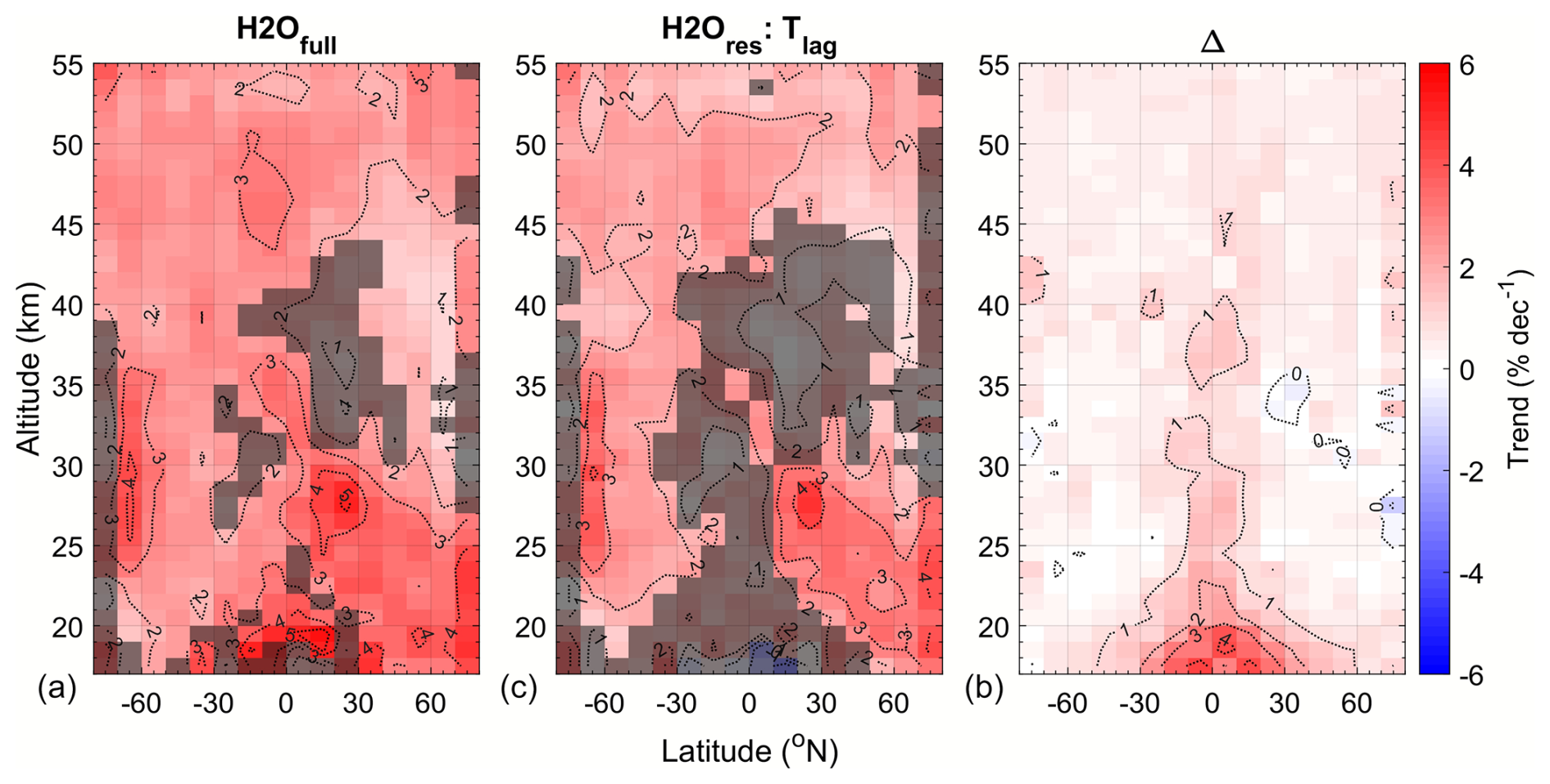
Figure 6 Same as Fig. 4, except the residual H₂O trends (b) are after regressing to ERA5 temperatures with empirically determined time lags (T_lag) and semi-annual and annual cycles.

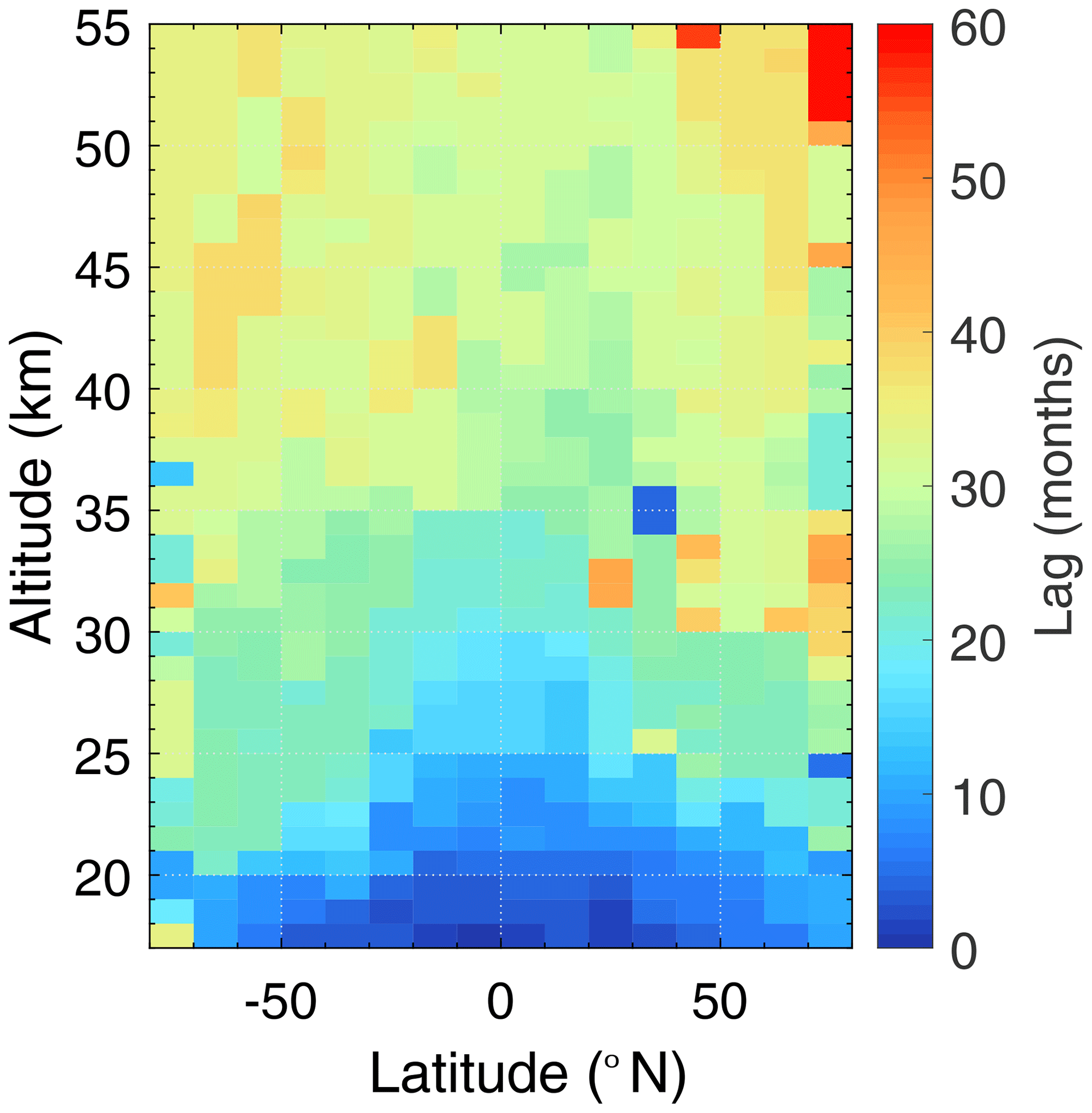
Figure 7 Lag times introduced to the ERA5 temperature time series (T_lag) that minimize the residuals between the ACE-FTS data and the MLR fit.

4.2 Accounting for CH₄ oxidation

In order to quantify how much CH₄ oxidation is contributing to stratospheric H₂O trends, firstly, local ACE-FTS CH₄ trends were calculated using an annual cycle, a semi-annual cycle, and ACE-FTS N₂O time series as regressors. As seen in the left panel of Fig. 8, the CH₄ trends are increasing in all regions and also exhibit a significant hemispheric asymmetry. In the mid- to high latitudes, NH CH₄ trends range from 3 % per decade in the lower stratosphere up to 12 % per decade near 55 km. These trends are greater than the SH trends that increase from 2 % per decade up to 8 % per decade. At the lower latitudes, hemispherical differences are only on the order of 1 %–2 % per decade, with relatively larger trends in the NH around 20–30 km and relatively larger trends in the SH around 40–55 km. The right panel of Fig. 8 shows how those trends contribute to the stratospheric H₂O via Eq. (3). The increases in CH₄ concentrations lead to an increase in the H₂O budget of ∼1 %–3 % per decade above ∼35 km and ∼1 %–2 % per decade below 35 km, with insignificant influence closer to the tropical tropopause region where there is expected to be little to no contribution from methane oxidation.

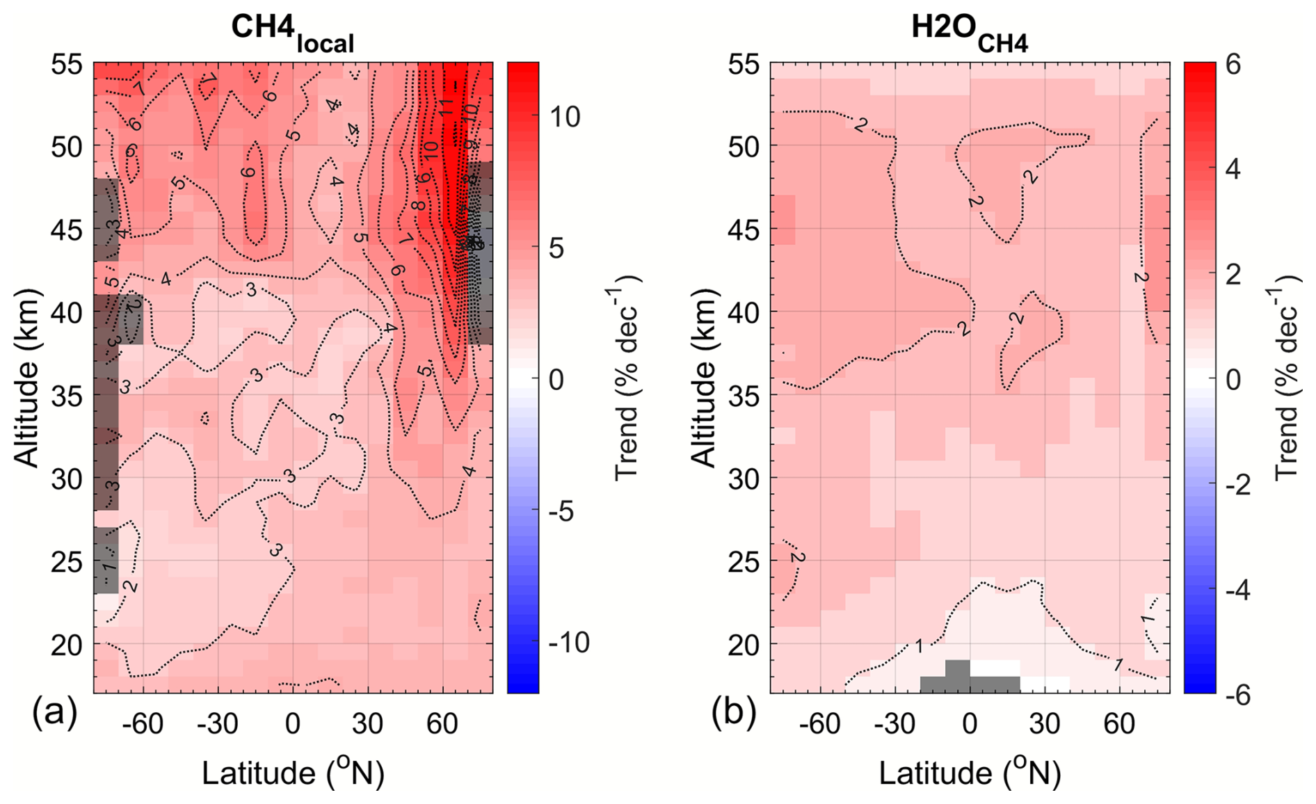
Figure 8 (a) ACE-FTS CH₄ local trends and (b) contribution of CH₄ oxidation to ACE-FTS H₂O trends. Shaded regions indicate regions with no significant trend to within 95 %.

As shown in Fig. 9, when ${\left[{\mathrm{H}}_{\mathrm{2}}\mathrm{O}\right]}_{{\mathrm{CH}}_{\mathrm{4}}}$ trends are subtracted from the residual H₂O trends that are calculated regressing to AO, SAO, N₂O, T_lag, and F10.7 cm time series, most of the trends throughout the stratosphere are within $\sim \pm \mathrm{1}$ % per decade and are not statistically significant. This indicates that these regressors can account for the full ACE-FTS H₂O trends throughout the majority of the stratosphere. The exceptions are in the mid- to high-latitude regions (∼30–70° S and 40–70° N) in the lower mid-stratosphere (∼20–35 km). In these regions, there are still significant residual H₂O trends of ∼1 %–2 % per decade. However, $\frac{\mathrm{d}[{\mathrm{CH}}_{\mathrm{4}}{]}_{\text{entry}}}{\mathrm{d}t}$ has not been constant over the past 20–30 years, as shown in Fig. 2. To account for this, a time-dependent trend analysis was performed on the CH₄ entry time series. Lagged 18-year trend values for the CMAM-ACE CH₄ entry time series were calculated for lag times of 0–10 years in 5 d intervals (i.e. a lag value of 10 years corresponds to the trend for 1994–2012). The calculated trends vs. lag times are shown in Fig. 10, and, as can be observed in Fig. 2, the 18-year CH₄ entry trends have been increasing since the early 1990s. This method of using lagged $\frac{\mathrm{d}[{\mathrm{CH}}_{\mathrm{4}}{]}_{\text{entry}}}{\mathrm{d}t}$ was employed by Hegglin et al. (2014). That study used time-lagged $\frac{\mathrm{d}[{\mathrm{CH}}_{\mathrm{4}}{]}_{\text{entry}}}{\mathrm{d}t}$ with lag times corresponding to the local mean age of air. However, ACE-FTS does not have validated measurements of age-of-air throughout the stratosphere; therefore the optimal lag times from the temperature regression (Fig. 7) are used as a proxy for mean age of air.

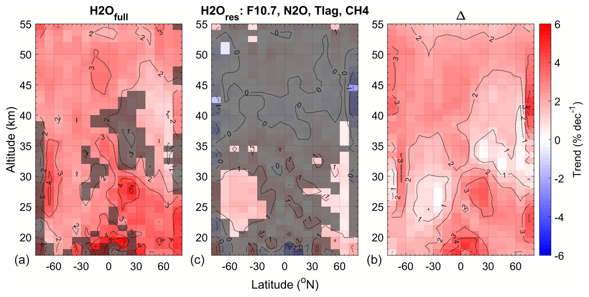
Figure 9 Same as Fig. 4, except the residual H₂O trends (b) are after regressing to semi-annual and annual cycles, F10.7 cm flux, and N₂O and T_lag time series and accounting for CH₄ oxidation.

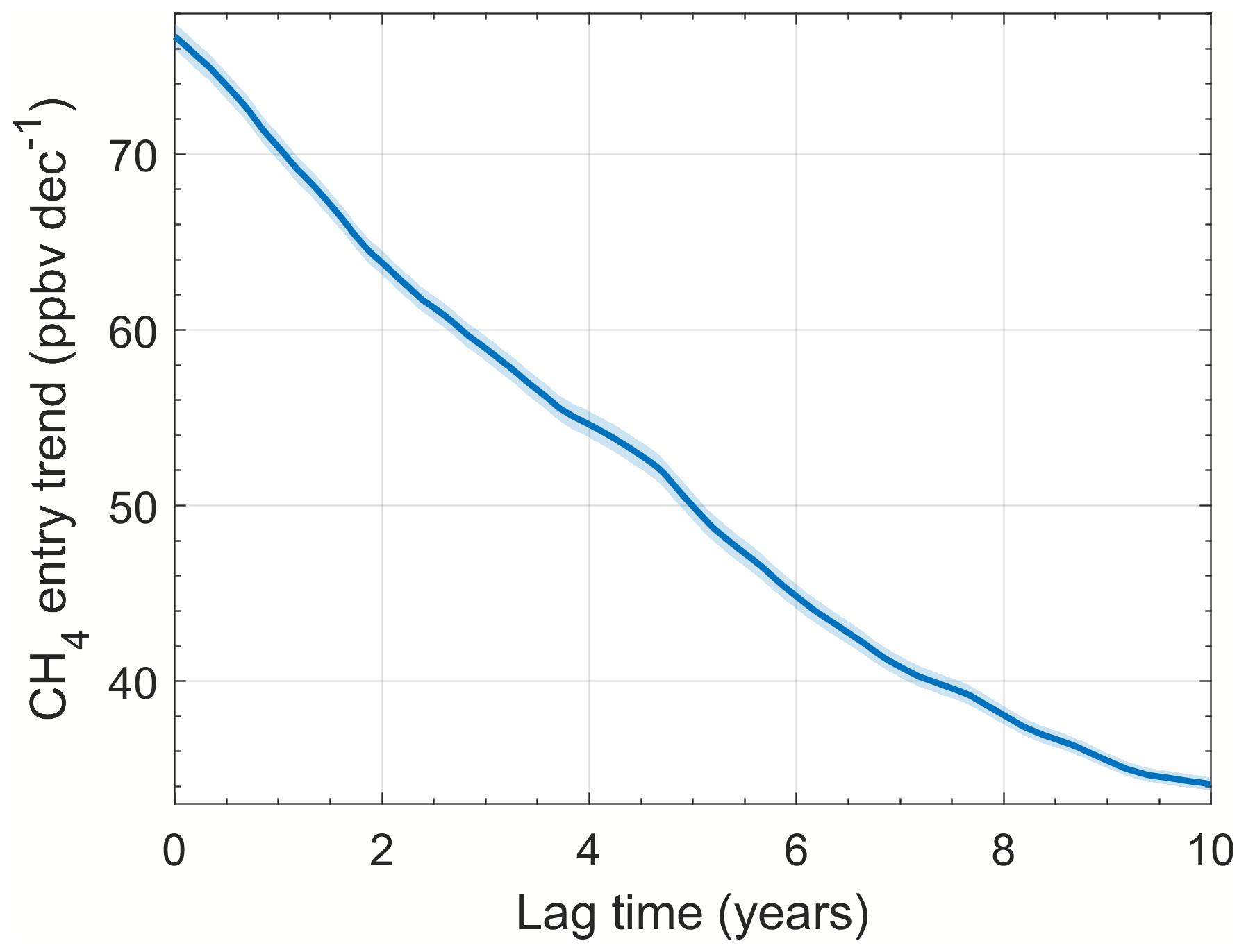
Figure 10 18-year CH₄ entry trends, as a function of lag time, for time periods of 1994–2012 (lag of 10 years) to 2004–2022 (lag of 0 years). The shaded region represents the 95 % confidence levels.

As expected, the H₂O trends due to CH₄ trends that account for time lags (Fig. 11) are less than those that use a constant CH₄ entry trend value (Fig. 8, right panel). Throughout the stratosphere, the CH₄ oxidation contribution leads to an ∼0.5 %–1.5 % per decade increase in H₂O, the larger of those trends tending to be throughout the SH and above ∼30 km in the NH.

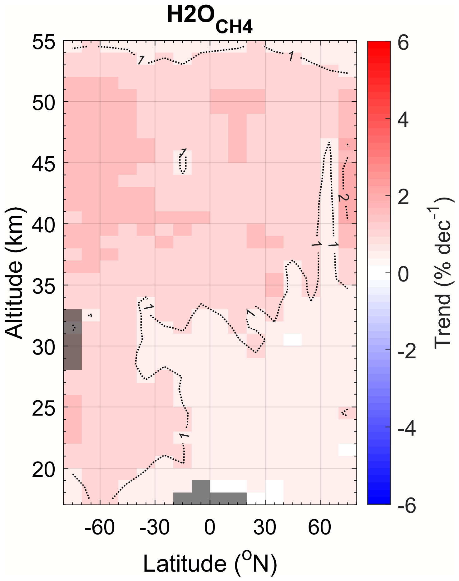
Figure 11 Trends in H₂O due to CH₄ oxidation using time-lagged CH₄ entry trend values (based on T_lag lag times).

In each altitude/latitude bin, the CH₄ oxidation contribution was determined using the lagged $\frac{\mathrm{d}[{\mathrm{CH}}_{\mathrm{4}}{]}_{\text{entry}}}{\mathrm{d}t}$ value that corresponds to that bin's lag time determined for T_lag (Fig. 7). The CH₄ oxidation contribution was then subtracted from that bin's residual H₂O trend that used AO, SAO, F10.7 cm, ACE-FTS N₂O, and T_lag time series as regressors. The final trend results for this method are shown in Fig. 12, and it can be seen in the middle panel that, when accounting for the non-linear increase in CH₄, there are more regions of the stratosphere where there are significant residual H₂O trends (than when assuming a constant increase). In the roughly 30–70° S, 20–35 km region, there remains a significant residual H₂O trend of 1.0 %–2.5 % per decade. The residual trend is smaller in the same altitude/latitude region in the NH, between 0.9 % and 1.7 % per decade, although, near 60° N, the region of significant trend extends up to 55 km. There is also a significant increase of ∼1 % per decade in parts of the SH low-latitude region above 45 km. These results indicate that there is at least one additional source of increasing H₂O in multiple regions within the stratosphere that has not been accounted for. It is likely that the regions with unaccounted-for trends are actually larger because, as discussed in Sect. 3, the lag times used to determine $\frac{\mathrm{d}[{\mathrm{CH}}_{\mathrm{4}}{]}_{\text{entry}}}{\mathrm{d}t}$ values only account for transit times from the entry point and do not account for mixing or differences in transit pathways (Poshyvailo-Strube et al., 2022). The effects on the regression results due to any correlation between the AO components and T_lag or N₂O are discussed in Appendix A2.

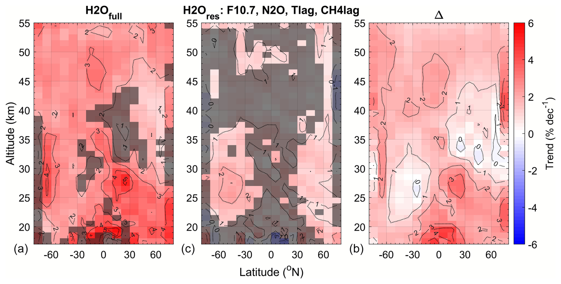
Figure 12 Same as Fig. 9, except time-lagged CH₄ entry trend values (based on T_lag lag times) were used when accounting for CH₄ oxidation.

As previously mentioned, Wrotny et al. (2010) determined that measurements are consistent with α having a value of up to 3.7 that could account for H₂O production via oxidation of H₂. Therefore, the H₂O trend calculation was done again using the same regressors (AO, SAO, N₂O, T_lag, F10.7 cm) and the time-lagged CH₄ entry trends but using a constant value of α=3.7 at all altitudes and latitudes. The results of the residual H₂O trends are shown in Fig. 13 and are not statistically significant in nearly every bin. It should be noted that the value of α is not changed in order to “optimize” the results; an extreme acceptable value was used simply to determine what effect that value would have on the calculated H₂O trends. Although it is unlikely that the maximum value of α=3.7 is appropriate for all altitudes and latitudes, these results indicate that this higher value of α could be consistent with the calculated ACE-FTS H₂O trends, especially in the mid-stratospheric extratropics, with the additional production due to increasing tropical tropospheric H₂ concentrations. In order to inform further analysis, a model study should be conducted investigating how H₂ concentrations have changed over the course of the ACE-FTS mission lifetime.

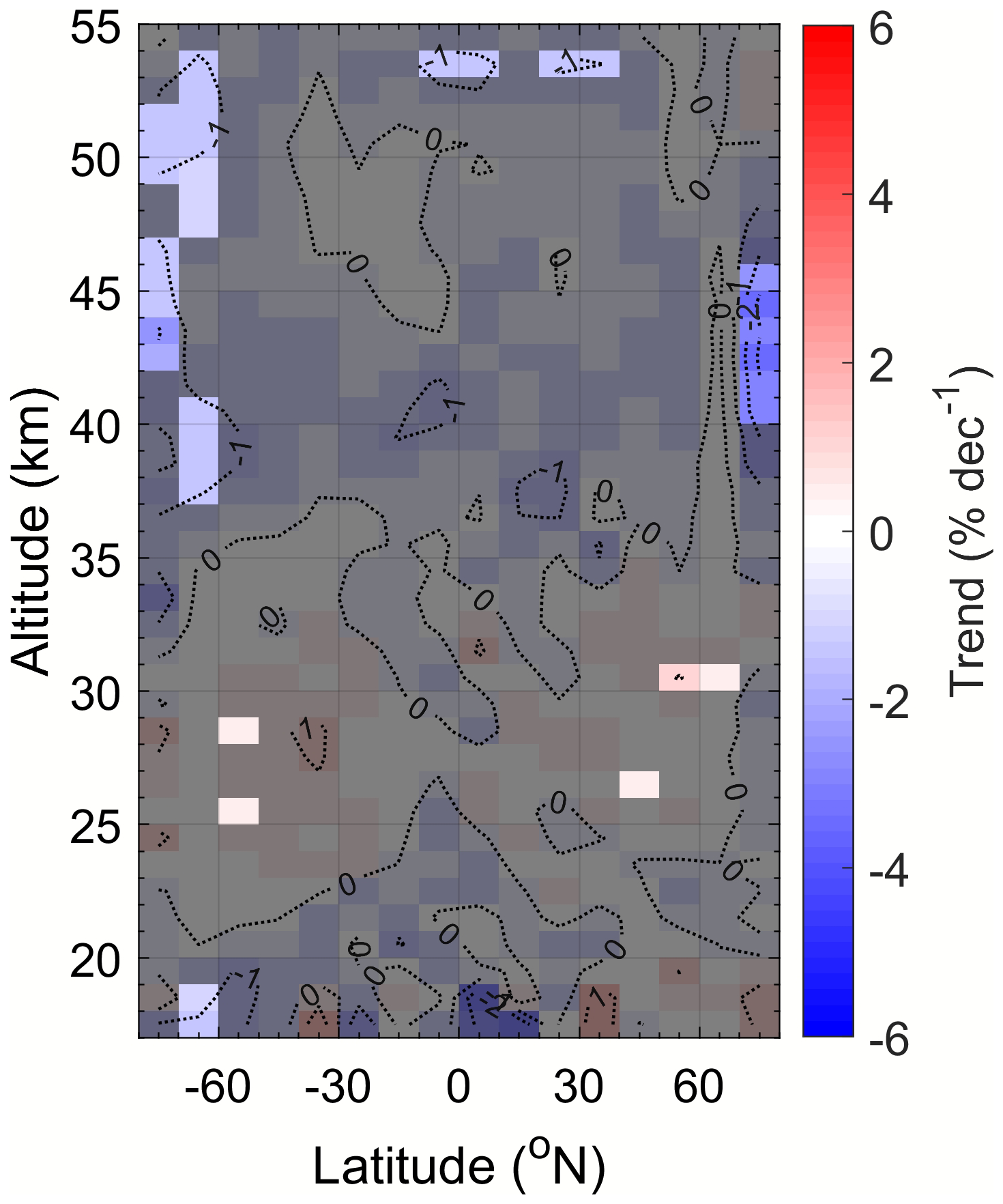
Figure 13 Residual H₂O trends after regressing to semi-annual and annual cycles, F10.7 cm flux, and N₂O and T_lag time series and accounting for CH₄ oxidation using time-lagged CH₄ entry values and an H₂O yield value of α=3.7 in all altitude/latitude bins. Shaded regions indicate regions with no significant trend to within 95 %.

One other source of stratospheric H₂O that has not been accounted for is convective moistening. In the troposphere, deep convection systems can transport ice particles into the tropopause region, and overshooting cloud tops can directly inject water vapour and ice into the lower stratosphere. Recent model studies (e.g. Dauhut and Hohenegger, 2022; Ueyama et al., 2023) have estimated that convective moistening contributes ∼10 % of the lower-stratospheric H₂O budget and can contribute up to ∼45 % in monsoon regions (Dessler and Sherwood, 2004; Hanisco et al., 2007; Tinney and Homeyer, 2021). Ueyama et al. (2023) estimated the global inter-annual variation in lower-stratospheric H₂O produced via deep convection between 2006 and 2016 to be on the order of a few percent (0.05–0.1 ppmv); however, the time period was too short to determine any significant trend. Further investigation is needed in order to determine if any longer-term changes in convection are influencing changes in stratospheric H₂O.

5 Conclusions

Measurements from ACE-FTS show that, between 2004 and 2022 H₂O, concentrations significantly increased at a rate of approximately 1 %–5 % per decade throughout nearly all of the stratosphere. This study uses ACE-FTS measurements of H₂O, CH₄, and N₂O, along with CMAM39 tropical upper-tropospheric CH₄ and ERA5 tropical tropopause temperatures, to quantify the relative contributions of different sources of these H₂O increases. The main sources are as follows:

• increasing tropical tropopause region temperatures. This is the main source of increasing H₂O in the tropical lower stratosphere. It accounts for H₂O increases of

  • ∼2 %–4 % per decade between 17 and 23 km in the tropics,

  • ∼1 %–2 % per decade between 23 and 50 km in the tropics, and

  • ∼1 %–2 % per decade 17–19 km in the mid-latitudes;

• structural BDC changes, which lead to

  • H₂O increases of ∼1 %–2 % per decade in NH mid-latitudes near 20–30 km and

  • H₂O decreases of ∼1 %–2 % per decade in SH mid-latitudes near 25–30 km and in NH mid-latitudes near 33–43 km;

• increasing CH₄ oxidation, which causes increases in H₂O on the order of

  • ∼1 %–2 % per decade above ∼30 km at all latitudes and above ∼20 km in the SH.

The solar influence on stratospheric H₂O was also investigated by regressing to F10.7 cm solar flux indices. Its contribution to the stratospheric H₂O trends was less than 0.5 % per decade in all altitude/latitude bins.

These sources combined account for all significant stratospheric H₂O trends except for a remaining ∼1 %–2 % per decade increase around 30–70° latitude in both hemispheres in the mid-stratosphere (∼20–35 km). These remaining trends can be accounted for by substituting the altitude-dependent CH₄ oxidation H₂O yield for a constant value of α=3.7 (upper limit from Wrotny et al., 2010), possibly indicating that these increases may be due to increasing concentrations of H₂, which also oxidizes to produce H₂O.

However, it remains that the measured stratospheric H₂O trends currently cannot be fully explained. As time goes on and more and more satellite limb-sounding missions are coming to an end, for the sake of continuity, it is vital that these types of atmospheric trends are fully understood – especially if there are going to be temporal gaps between the operational periods of current and future instruments. There is an urgent need for new satellite missions to continue this observational record to enable more reliable trend estimation and for model studies to determine what influences changes in processes such as H₂ oxidation and deep convection – and other possible sources – have on the stratospheric regions where the full H₂O trends cannot be fully accounted for.

Appendix A

A1 Time-lagged ENSO and tropopause pressure

The effects of ENSO conditions and tropopause pressure on stratospheric H₂O, however, are not instantaneous. Similarly to the time-lagging method described in Sect. 3, the ENSO and trop time series were lagged to find lag times in each bin that maximize the correlations between local H₂O and the respective index time series. The influence of lagged ENSO and lagged trop on H₂O trends is shown in the top panel of Fig. A1, and the respective corresponding optimal lag times in months are shown in the bottom panel. The influence of both lagged ENSO and lagged trop is still typically less than 1 % per decade throughout the stratosphere.

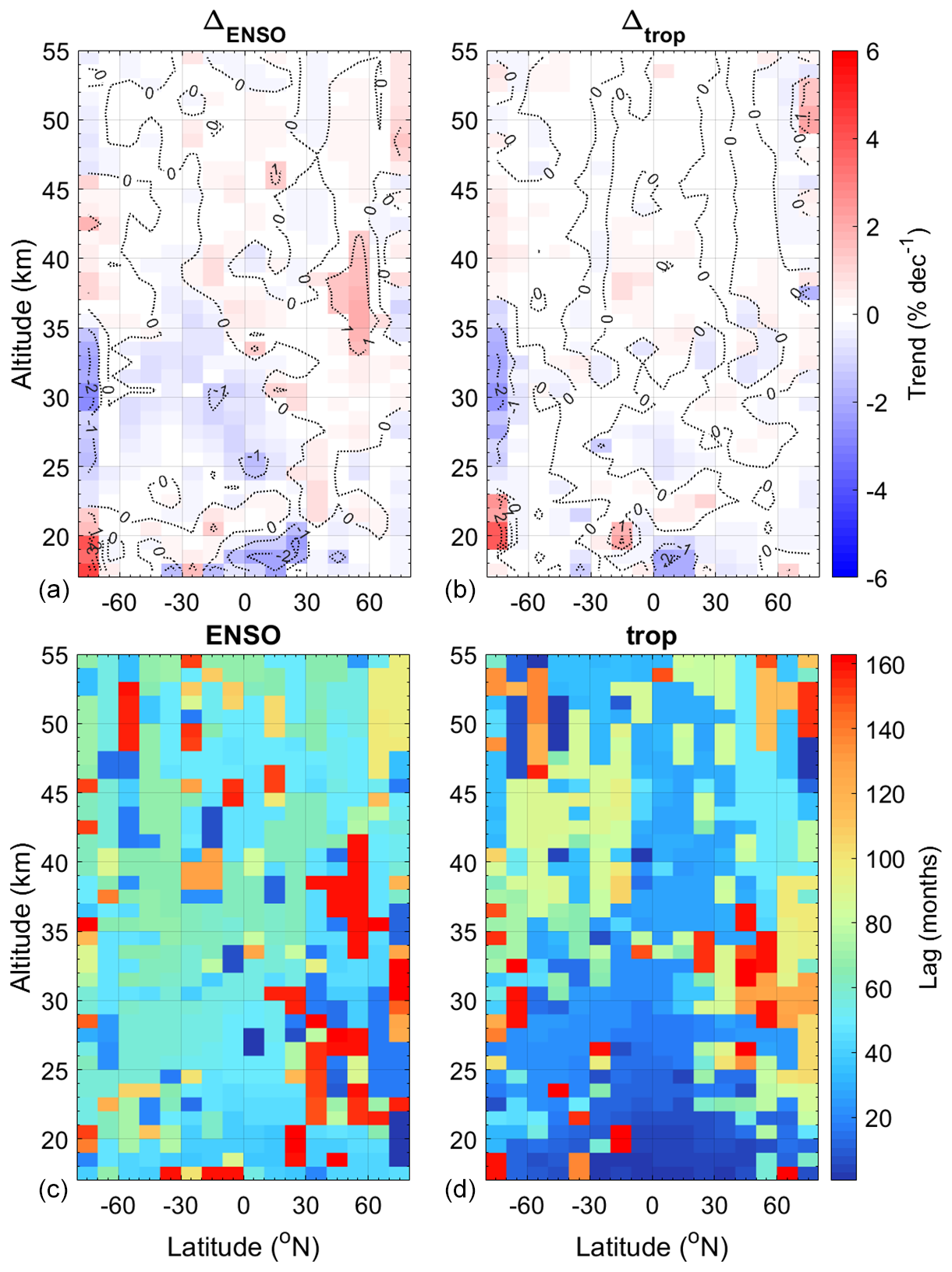
Figure A1 (a, b) The difference between the full trends and the residual trends when regressing to the lagged ENSO and trop time series and semi-annual and annual cycles. (c, d) The corresponding optimal lag times.

A2 Correlation with AO

When accounting for CH₄ oxidation with time-lagged entry trends and regressing to T_lag, N₂O, SAO, and no AO components, the resulting residual trends are not meaningfully different below ∼42 km from the same case with AO included as a regressor, as seen in Fig. A2. The main differences are above 42 km. Without including AO, the region with significant residual trends in the low mid-latitudes is larger but still on the order of 1 % per decade, the SH high latitudes exhibit negative residual trends on the order of −1 % per decade, and the NH mid- to high latitudes exhibit no significant trends. Therefore, further study is still needed to fully parse the H₂O trends in the upper stratosphere.

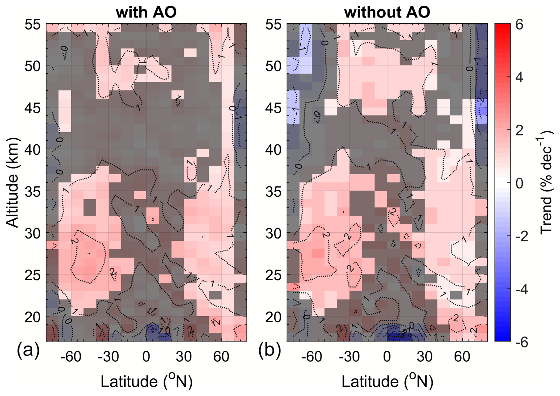
Figure A2 (a) Residual H₂O trends after regressing to semi-annual and annual cycles, F10.7 cm flux, and N₂O and T_lag time series and accounting for CH₄ oxidation using time-lagged CH₄ entry values. (b) Same as panel (a) but without regressing to annual cycles. Shaded regions indicate regions with no significant trend to within 95 %.