Marine emissions and trade winds control the atmospheric nitrous oxide in the Galapagos Islands

Nitrous oxide (N₂O) is a potent greenhouse gas emitted by oceanic and terrestrial sources, and its biogeochemical cycle is influenced by both natural processes and anthropogenic activities. Current atmospheric N₂O monitoring networks, including tall-tower and flask measurements, often overlook major marine hotspots, such as the eastern tropical Pacific Ocean. We present the first 15 months of high-frequency continuous measurements of N₂O and carbon monoxide from the newly established Galapagos Emissions Monitoring Station in the region. Over this period, N₂O mole fractions vary by approximately 5 ppb, influenced by seasonal trade winds, local anthropogenic emissions, and air masses transported from marine N₂O emission hotspots. Notably, between February and April 2024, we observe high variability linked to the southward shift of the intertropical convergence zone and weakened trade winds over the Galapagos Islands. Increased variability during this period is driven by stagnant local winds, which accumulate emissions, and the mixing of air masses with different N₂O contents from the Northern Hemisphere and the Southern Hemisphere. The remaining variability is primarily due to differences in air mass transport and heterogeneity in surface fluxes from the eastern tropical Pacific. Air masses passing over the Peruvian and Chilean upwelling systems – key sources of oceanic N₂O efflux – show markedly higher N₂O mole fractions at the station.

1 Introduction

Nitrous oxide (N₂O) is a potent greenhouse gas with the fourth-largest effective radiative forcing increase since industrialization, equating to 0.21 W m⁻², and is, additionally, an ozone-depleting substance in the stratosphere (Forster et al., 2021; Ravishankara et al., 2009). The mean tropospheric growth rate of N₂O between 1995 and 2019 is reported to be 0.85 ± 0.03 ppb yr⁻¹ and is accelerating (Canadell et al., 2021; Dutton et al., 2024; Francey et al., 2003; Prinn et al., 2018). Natural processes dominated by ocean and soil microbial metabolisms, namely denitrification and nitrification, account for the majority of N₂O sources to the atmosphere (Tian et al., 2024). Globally integrated marine N₂O emissions are estimated to be 3.1–6.3 Tg N yr⁻¹ (Canadell et al., 2021; Tian et al., 2024), with coastal waters contributing to much of this flux (Resplandy et al., 2024). Moreover, data-informed studies tend to report higher marine emissions than biogeochemical models alone (Resplandy et al., 2024; Tian et al., 2024; Yang et al., 2020). Oxygen-minimum zones, characterized by less than 60 µmol kg⁻¹ oxygen content (Stramma et al., 2008), and eastern boundary coastal upwelling systems are hotspots of marine N₂O emissions, accounting for approximately 22 % of oceanic emissions (Yang et al., 2020). Yet, the accuracy of these marine estimates has been limited by poor spatial and temporal resolutions of ship-based observations. Moreover, different techniques for emission estimation, such as direct flux calculations based on air–sea concentration gradients versus flux calculations using atmospheric inverse modeling, are difficult to reconcile due to inherent methodological biases and varying assumptions, such as the gas transfer velocity parameterization (Wanninkhof, 2014). Marine emissions – particularly in the eastern tropical Pacific, characterized as one of the largest marine N₂O sources – are further impacted by the El Niño–Southern Oscillation (ENSO) through the modulation of coastal nutrient upwelling that supports surface productivity (Babbin et al., 2020; Ji et al., 2019; Thompson et al., 2013, 2019). Reduced upwelling during an El Niño restricts productivity and consequently reduces the magnitude of low-oxygen environments in the subsurface where N₂O is produced. The isolation of low-oxygen surface environments from the surface due to increased stratification during an El Niño event could lead to subsurface accumulation of N₂O (Ji et al., 2019). However, the effect of subsurface accumulation on subsequent surface fluxes still needs to be explored.

Long-term and high-frequency monitoring of atmospheric greenhouse gases, including N₂O, with flask samples or tall-tower measurements has enabled the exploration of tropospheric growth rates and global emissions estimates with a top-down approach for decades (Hirsch et al., 2006; Patra et al., 2022; Saikawa et al., 2014; Stell et al., 2022; Thompson et al., 2014, 2019; Wells et al., 2015, 2018). Yet, the investigation of regional N₂O surface fluxes or air–sea interface disequilibrium in the literature has highlighted the importance of atmospheric monitoring near emission sources (Babbin et al., 2020; Ganesan et al., 2015, 2020; Jeong et al., 2018; Nevison et al., 2018, 2023; Saboya et al., 2024). Despite the significance of the eastern tropical Pacific as a hotspot of oceanic N₂O emissions, with a strong correlation with ENSO (Babbin et al., 2015, 2020; Bange et al., 1996; Ji et al., 2019; Martinez-Rey et al., 2015), there have been no continuous high-frequency atmospheric N₂O monitoring sites in the region (Fig. 1a). Current estimates of N₂O emissions from the area rely on direct measurements during sporadic oceanographic expeditions (Arevalo-Martínez et al., 2015; Buitenhuis et al., 2018; Nevison et al., 1995) and ocean-based statistical or biogeochemical models (Landolfi et al., 2017; McCoy et al., 2023; Suntharalingam et al., 2000; Yang et al., 2020). However, the direct surface flux measurements are temporally and spatially sparse (Bange et al., 2019).

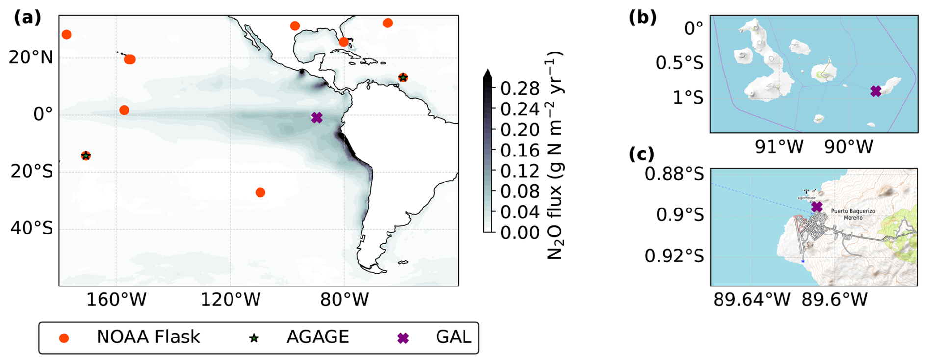
Figure 1 (a) Global atmospheric nitrous oxide monitoring network in relation to the ocean-based and observationally driven nitrous oxide fluxes from Yang et al. (2020). Orange circles signify NOAA Global Greenhouse Gas Reference Network flask air sample measurement sites (Lan et al., 2024). Green stars signify Advanced Global Atmospheric Gases Experiment (AGAGE) network sites (Prinn et al., 2018). (b, c) Maps of the Galapagos Islands and the island of San Cristóbal, respectively, with the location of the Galapagos Emissions Monitoring Station (GAL) marked using a purple X. © OpenStreetMap contributors 2024. Distributed under the Open Data Commons Open Database License (ODbL) v1.0.

Located in the eastern tropical Pacific Ocean, the Galapagos Islands are situated in proximity to the hotspots of oceanic N₂O emissions: the Peruvian and Chilean upwelling systems (Fig. 1a). Therefore, the Galapagos Islands are potentially ideal for monitoring atmospheric N₂O trends in a region where previous direct observations are lacking. Prevailing winds over the Galapagos consist of southeasterly trade winds, transporting air masses from the western coast of South America to the Galapagos most of the year (Forryan et al., 2021). Throughout the year, the temperature remains between 22–26 °C, with the maximum precipitation and more stagnant winds being observed in February and March (Paltán et al., 2021). During the wet season (January–May), the winds are dominantly easterly due to the southward shift of the intertropical convergence zone (ITCZ) over the eastern Pacific (Risien and Chelton, 2008). Therefore, the seasonality of the winds over the Galapagos creates an opportunity to potentially capture the atmospheric greenhouse gas differences from both hemispheres and record regions of high N₂O emissions in the eastern Pacific.

Despite the significance of the Galapagos Islands' location in the tropical Pacific Ocean for climate research, atmospheric monitoring on the islands has been limited to short-term campaigns focusing on atmospheric pollutants such as particulate matter or ozonesonde deployments at monthly intervals. NASA AERONET (Aerosol Robotic Network) has been active in the Galapagos since 2017, allowing for the identification of baseline aerosol conditions, as well as of local air pollution episodes (Cazorla and Herrera, 2020). Similarly, other studies have investigated the role of marine aerosols in the local air quality and their transport from the eastern tropical South Pacific Ocean (Gómez Martín et al., 2013; Sorribas et al., 2015). However, no long-term monitoring studies exist for greenhouse gases, such as N₂O, in the Galapagos.

Here, we present high-frequency and continuous N₂O and CO atmospheric mole fraction observations from the Galapagos Emissions Monitoring Station. In this study, we investigate the observed variability in the mole fractions between July 2023 and September 2024 and attribute the variability to changes in local meteorology and regional emissions at synoptic timescales. Akin to previous studies at various atmospheric measurement stations for greenhouse gases and atmospheric pollutants (Ganesan et al., 2013; Grant et al., 2010; Tohjima et al., 2002; Thompson et al., 2009; Zhang et al., 2011), this study aims to advance the understanding of trends in N₂O mole fractions and to inform future top-down estimates of regional and global emissions that combine atmospheric transport and inverse models with atmospheric observations. Because such top-down analyses cannot resolve emissions for the grid cell in which observations are collected, it is necessary to identify periods during which local emissions are a possible dominant source of N₂O. Given the availability of concurrent CO measurements due to instrumental capabilities, we supplement the analysis of N₂O variability with CO data to examine the influence of local anthropogenic activities. Additionally, we analyze the stagnancy of sampled air masses using supplementary meteorological data to further refine the observations. Lastly, investigating the N₂O and CO diurnal cycles is necessary as they provide insights into how local trends in anthropogenic activities in the Galapagos impact short-term observations.

2 Methods

2.1 Site description and sampling setup

The Galapagos Emission Monitoring Station (GAL) is located on the island of San Cristóbal in the Galapagos Islands, Ecuador. It is situated in the eastern Pacific Ocean at 0.89562° S and 89.60866° W. The instruments are housed in the Terrestrial Ecology Laboratory at the Galapagos Science Center, operated by the Universidad San Francisco de Quito and the University of North Carolina, Chapel Hill. The station is located in the northern part of Puerto Baquerizo Moreno, a city with a population of approximately 7000, on San Cristóbal and at the edge of the Galapagos National Park (Fig. 1c). Additionally, the Galapagos Science Center (GSC) is equipped with a weather station that measures temperature, wind speed and direction, relative humidity, and precipitation at 5 min intervals.

Ambient air is pumped through the sampling line with an inline vacuum pump (ALITA Industries, AL-6SA) at 10 L min⁻¹ through Monel mesh fitted inside an inverted stainless steel sampling cup. Monel (a nickel–copper alloy) mesh prevents coarser materials from entering the sampling line. The sampling inlet is located on the roof of the Galapagos Science Center at 27 ± 1 m above sea level (17 ± 1 m above ground level). Ambient air is pulled through a $\mathrm{1}/{\mathrm{4}}^{\prime \prime }$ Eaton Synflex 1300 polyethylene–aluminum composite tubing. Inside the laboratory, the air sampling line is heated to 35 °C using a heating cable operated by a temperature controller (CAL Controls, CAL3300). Once in the lab, air samples are pulled from the main Eaton Synflex line using a tee connector attached to a 7 µm stainless steel mesh filter at a rate of 0.1 L min⁻¹. The ambient versus calibration air flow is switched via the Picarro Inc. A0311 16-Port Distribution Manifold. After the manifold, humidity in the sample is removed using a Nafion™ tubing dryer (Perma Pure Inc.) housed inside a custom temperature-controlled enclosure. The Nafion™ dryer is used in reflux mode where out-flowing air from the analyzer is used as a counter purge to dry the inflow (Fig. S1 in the Supplement) (Welp et al., 2013). The temperature of the drying box is set to 35 °C using an OMEGA iSeries temperature controller. Additionally, the air pressure is set to 0.8 atm using a pressure controller (Alicat Inc., PC Series 15-PSIA) inside the drying box. After the drying and pressure control, the air sample is filtered through a 2 µm stainless steel mesh before being introduced into the analyzer. While the 7 µm filter removes any large impurities in the main sampling line before the 16-port distribution manifold, an additional 2 µm filter is necessary upstream of the analyzer to prevent any finer impurities from entering the ultra-clean cavity. The mole fractions of N₂O, CO, and H₂O are measured with a Picarro Inc. G5310 cavity ring-down spectroscopy analyzer. The flow diagram for air sampling and measurements is illustrated in Fig. S1. All tubing is 316 stainless steel fitted with 316 stainless steel compression fittings (Swagelok). Similar setups have been employed at various atmospheric greenhouse gas monitoring sites (Andrews et al., 2014; Prinn et al., 2018; Stanley et al., 2018).

2.2 Mole fraction measurements and calibrations

The atmospheric composition of the air samples, i.e., the mole fraction of N₂O, CO, and H₂O, is measured by a Picarro G5310 cavity ring-down spectroscopy (CRDS) analyzer. Due to overlapping spectral features of N₂O and CO absorption in the near-infrared (IR) range and their relevance to climate and air quality monitoring, the Picarro Inc. G5310 CRDS provides concurrent measurements of both gases (Adkins et al., 2021; Nie et al., 2024; Zellweger et al., 2019). The air samples are dried prior to measurement to minimize the biases in the dry-air mole fraction calculations performed by the native Picarro G5310 software, as described in previous studies (Rella, 2010; Reum et al., 2019; Zellweger et al., 2019). No further water vapor corrections are performed as the mean measured H₂O mole fraction was 775 ± 100 ppm (1 SD) due to the inline Nafion™ tubing dryer. Mole fraction measurements are obtained every 4–10 s, but 1 min means and standard deviations are reported. The measurements are calibrated by sampling four calibration tanks at various time intervals.

All the calibration tanks are certified at the NOAA Global Monitoring Laboratory (GML) following the WMO-N₂O_X2006A and WMO-CO_X2014A calibration scales (Hall et al., 2007; Novelli et al., 1991). For this study, each calibration tank is named based on its use during the calibration process. The standard tank (CC746185; 333.82 ppb N₂O, 136.3 ppb CO) is sampled for 20 min daily. A calibration sequence with a high-calibration tank (CC746187; 347.54 ppb N₂O, 299.1 ppb CO) and a low-calibration tank (CC746176; 326.54 ppb N₂O, 53.9 ppb CO) is performed once per month. A mid-range-calibration tank, also referred to as the target tank (CC746233; 340.20 ppb N₂O, 163.4 ppb CO), is sampled once per week to evaluate long-term instrument performance. The standard deviation of each measurement session is also used to estimate the repeatability metric for the GAL sampling and measurement setup, as illustrated in Fig. S2. Based on the average standard deviation of all the measurement sessions for each calibration tank, we report the repeatabilities of N₂O and CO to be 0.04 and 0.40 ppb, respectively. The repeatability for N₂O is sufficient to assess the precision of our measurements and is comparable to other high-frequency monitoring stations, with reported repeatabilities between 0.03 and 0.66 ppb (Ganesan et al., 2013; Labuschagne et al., 2018; Lebegue et al., 2016; Stanley et al., 2018). Similarly, N₂O flask measurements from the NOAA Global Greenhouse Gas Reference Network have repeatability ranging between 0.01 and 0.02 ppb based on repeated measurements of the high-calibration tank (Lan et al., 2024). The sampling sequences, instrumental drift calculations, and calibrations are controlled and performed by GCWerks™ software (https://www.gcwerks.com, last access: 25 May 2023). The software is widely utilized by various atmospheric monitoring networks such as AGAGE (Prinn et al., 2018) or the UK Deriving Emissions linked to Climate Change (UK DECC) network (Stanley et al., 2018; Stavert et al., 2019).

For the calibration calculation, the drift-corrected mole fraction, χ, is calculated following Eq. (1), where χ_std refers to the reported value of the standard tank, and m and m_std refer to the measured dry mole fractions of ambient air and the standard tank, respectively. Furthermore, during calibration sessions, non-linearity calculations are performed based on drift-corrected mole fraction values of high- and low-calibration tanks. A linear (for N₂O) or quadratic (for CO) relationship between the ratio-to-standard and drift-corrected sensitivity (S_drift) is determined for three calibration tanks following Eq. (2). These functional forms are selected per common practice (Stanley et al., 2018) because they minimize the R² value for the calibration tank non-linearity correction fits, as shown in Fig. S3. As a result, the drift-corrected ambient air mole fraction values are scaled using the determined non-linearity expression for each gas to obtain the reported mole fractions. Post-calibration results from the repeated measurements of these calibration tanks are provided in Fig. S4 to highlight the long-term stability of the measurement and calibration methods.

$$\begin{array}{}\text{(1)}& {\displaystyle }\mathit{\chi }={\mathit{\chi }}_{\mathrm{std}}{\displaystyle \frac{m}{m_{\mathrm{std}}}}\text{(2)}& {\displaystyle }{S}_{\mathrm{drift}}={\displaystyle \frac{\frac{{\mathit{\chi }}_{\mathrm{tank}}}{m_{\mathrm{tank}}}}{\frac{{\mathit{\chi }}_{\mathrm{std}}}{m_{\mathrm{std}}}}}\end{array}$$

2.3 Air mass footprint calculations with FLEXPART Lagrangian particle dispersion model

To estimate the transport history of the air masses sampled at GAL, we use a Lagrangian particle dispersion model, FLEXPART v10.4 (Flexible Particle Dispersion Model) (Pisso et al., 2019; Stohl et al., 1998, 2005). FLEXPART calculates the location of inert particles in the atmosphere from a Lagrangian perspective, given the wind speeds and direction over time. In this study, we release 50 000 particles every 3 h from the station at 27 m above sea level and follow them 20 d backward in time within a domain between 50° S to 31° N and 40 to 121° W. The meteorology used for the FLEXPART model is the European Centre for Medium-Range Weather Forecasts (ECMWF) ERA5 reanalysis product with a lateral resolution of 31 km × 31 km (approximately 0.28125° × 0.28125° for our equatorial site) and 37 vertical pressure levels (Hersbach et al., 2023). The lateral resolution of the FLEXPART model is selected to match that of ERA5. The footprints (F; $\mathrm{s}{\mathrm{kg}}^{-\mathrm{1}}\mathrm{pmol}{\mathrm{mol}}^{-\mathrm{1}}$), i.e., the source–receptor relationship, within the 0–100 m range above sea level over the full domain were used for further analysis (Henne et al., 2016; Pisso et al., 2019; Seibert and Frank, 2004; Stohl et al., 2009). Footprints represent the sensitivity of measured N₂O mole fractions at GAL (in pmol mol⁻¹) to fluxes across some land or ocean surface (in kg s⁻¹).

We define a regional influence term I based on the calculated footprints for each 3-hourly release, as shown in Eq. (3). This term helps to examine the role of transport from different regions within the domain in modifying the observed N₂O concentrations. The regions considered include (i) the Peruvian and Chilean upwelling systems, as previously defined by Yang et al. (2020); (ii) the Northern Hemisphere; and (iii) a 3 × 3 grid cell area centered on GAL. All three regions are illustrated in Fig. 2. While the areal extent of the three regions differs significantly, they serve as analytical tools for further analyzing which mechanisms could explain the observed variability in N₂O over the Galapagos. Each region is indicated by the subscript r, with an associated two-dimensional lateral matrix R to describe the region. In this context, the subscripts i and j indicate latitude and longitude, while t represents the 3-hourly time period when FLEXPART footprints are computed. The matrix R is a binary matrix containing only 0 and 1 values to define a region spatially; therefore, multiplying it with the footprint matrix zeroes out all footprint values outside the defined region. Consequently, the regional influence term I_r,t represents the fraction of air masses transported over a specific region relative to the cumulative footprint at a given time. Overall, this metric helps identify how much of the observed N₂O variability can be attributed to air mass transport over each defined region. The histograms for each regional influence metric are provided in Fig. S5.

$$\begin{array}{}\text{(3)}& I_{\mathrm{r},\mathrm{t}}={\displaystyle \frac{{\sum }_{i,j}{F}_{i,j,t}\cdot R_{i,j}}{{\sum }_{i,j}{F}_{i,j,t}}}\end{array}$$

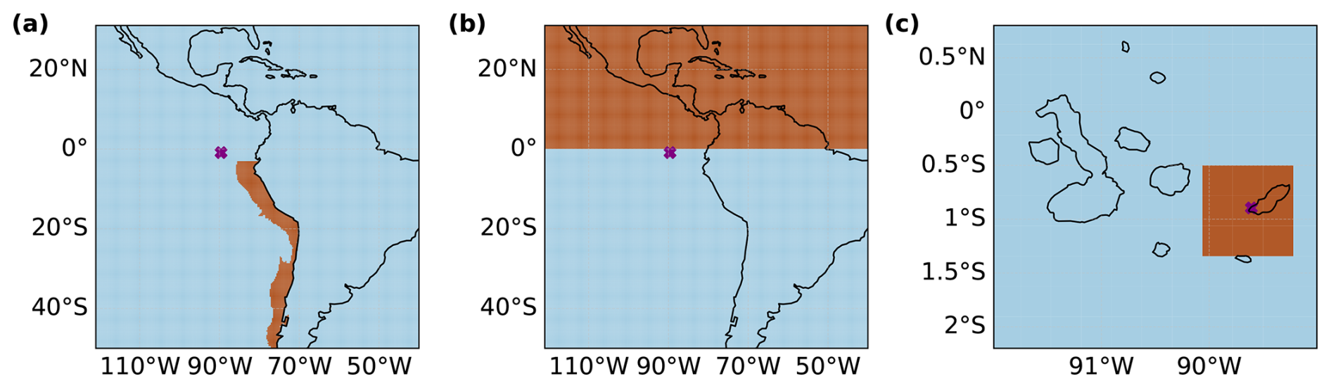
Figure 2 Definitions of the regional influence metrics for (a) the Peruvian and Chilean upwelling systems (I_upw) based on Yang et al. (2020), (b) the Northern Hemisphere (I_NH), and (c) a local 3 × 3 grid centered on GAL (I_local). Each region is highlighted in orange, with the Galapagos Emissions Monitoring Station indicated by a purple X.

3 Results and discussion

3.1 N₂O and CO observations in the Galapagos

The atmospheric mole fraction of nitrous oxide (N₂O) and carbon monoxide (CO) has been measured continuously since July 2023 at the Galapagos Emissions Monitoring Station. Figure 3 shows a time series of the 3-hourly averages of the mole fraction measurements. N₂O observations are juxtaposed with monthly mean mole fractions from other high-frequency tall-tower or flask measurement sites in the Pacific or tropical Atlantic. Over the first year, the observed N₂O mole fraction in the Galapagos varies between 336.53 and 341.45 ppb, with an annual growth rate of 1.82 ± 0.45 ppb yr⁻¹. This growth rate is calculated as the average difference for days measured in both 2023 and 2024, and it is comparable to the global growth rate in 2021, which was 1.38 ppb yr⁻¹ (Tian et al., 2024). The annual growth rate in the Galapagos is likely to be overestimated due to the lack of multiple months of continuous data availability during both years and the potential impact of emissions-related synoptic N₂O enhancements. Moreover, the growth rate in the Galapagos is higher compared to the 2010–2019 average (Canadell et al., 2021) because it includes interannual variability of natural N₂O sources in the eastern Pacific Ocean. During 2023, the observed monthly mean N₂O closely follows the trends illustrated by flask measurements at the Mauna Loa, Hawaii, and Ragged Point, Barbados, stations. On the other hand, monthly mean N₂O mole fractions observed at Kennaook/Cape Grim, Australia, are, on average, 1.30 ppb lower than the Galapagos observations. This difference could be explained by the inter-hemispheric difference in N₂O mole fractions (Prinn et al., 2018) and by low N₂O fluxes from the Southern Ocean and Antarctic regions over which the air masses sampled at Kennaook/Cape Grim are transported (Wilson et al., 1997). The average N₂O deviation from a monthly mean during the wet season is 0.73 ppb, whereas it is 0.34 ppb during the dry season. The increase in the variability can be attributed to changes in local and regional wind patterns and meteorology, which will be discussed in more detail later.

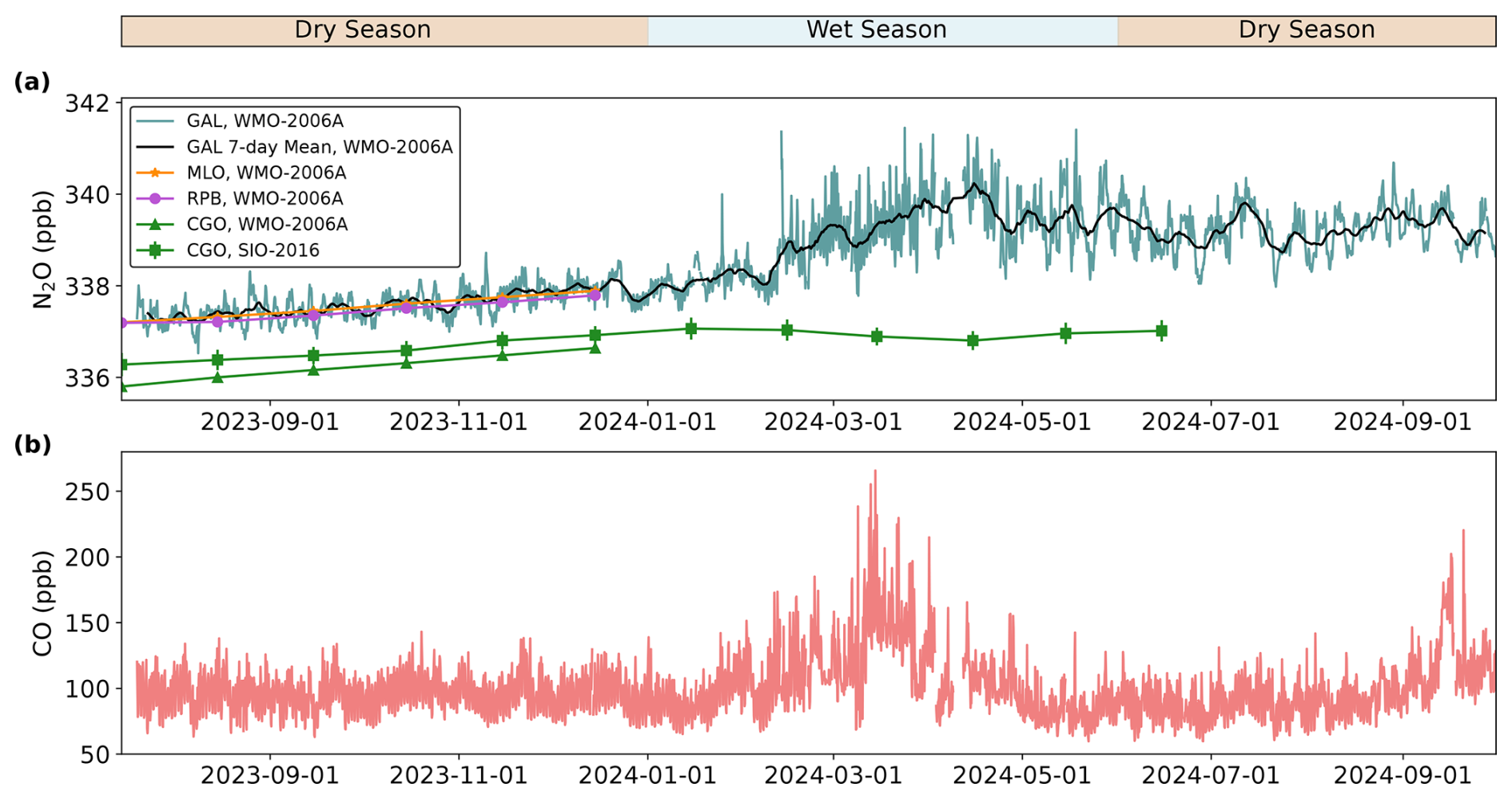
Figure 3 The 3-hourly average of (a) nitrous oxide (N₂O) and (b) carbon monoxide (CO) mole fractions at the Galapagos Emissions Monitoring Station (represented with a three-letter acronym, GAL) during the first year of measurements. A 7 d running mean time series for GAL N₂O observations is plotted in black. N₂O mole fractions are compared to monthly averages of the stations such as Mauna Loa, Hawaii Observatory (MLO, orange); Ragged Point, Barbados Observatory (RPB, purple); and Kennaook/Cape Grim, Australia Observatory (CGO, green), with two different calibration scales. Measurements calibrated with the NOAA-2006A scale are monthly mean values from NOAA Global Greenhouse Gas Reference Network flask air sample measurements (Lan et al., 2024). In contrast, the CGO SIO-2016 monthly averages represent the high-frequency atmospheric monitoring station operated by the CSIRO and AGAGE networks in Kennaook/Cape Grim (Prinn et al., 2018). Dates are shown in YYYY-MM-DD format. The average 3-hourly standard deviations of N₂O and CO are 0.16 and 3.77 ppb, respectively. Since 1-standard-deviation error bars are small compared to the 3-hourly averages, they are not plotted for GAL observations. The color bar above shows the dry season in tan and the wet season in light blue, designated based on climatological precipitation in San Cristóbal (Paltán et al., 2021).

Alongside N₂O, CO mole fractions are monitored at GAL. While 3-hourly averaged CO measurements range between 59–266 ppb, no significant annual growth is observed over the Galapagos. The average mole fraction of CO, excluding the highly variable wet season, is 96 ± 22 ppb. This agrees with a previous study that reports the baseline CO mole fraction as 80 ppb, with two peaks in March–April and August–September (Cazorla and Herrera, 2020), over the Galapagos based on MOPITT satellite observations. While the increased CO mole fraction in March–April aligns with our observations, no significant increase in CO mole fraction was observed in September 2023. Cazorla and Herrera (2020) attribute the large CO peak in September to the transport of air masses from the Amazon basin during a large biomass burning season. However, such attributions were supported by air mass back trajectory calculations at 1500–5000 m above sea level, whereas the observations at GAL represent the lower-altitude surface mixed layer. We observe increased CO in September 2024, which might be related to large-scale combustion, but further studies are required for such attribution. In addition to its importance for air quality, carbon monoxide mainly indicates local fuel combustion or biomass burning events that could also indicate increased atmospheric N₂O mole fractions (Bray et al., 2021; Cofer III et al., 1991). Therefore, further discussion of CO variability is only included to support the examination of variability in N₂O observations in the following sections.

3.2 Diurnal variability

In Fig. 4, the diurnal cycles of N₂O and CO mole fractions are represented as the average anomaly from the daily mean at each hour. The amplitude of diurnal variability for N₂O is 0.16 ppb, approximately 0.05 % of the observed average N₂O mole fraction. However, the N₂O diurnal-cycle standard deviation is much larger than the amplitude due to strong synoptic variability in N₂O observations. The peak mean N₂O anomaly is observed at 12:00 UTC (06:00 local time), and the lowest mean N₂O anomaly is observed at 22:00 UTC (16:00 local time). The diurnal trend is approximately sinusoidal, with decreasing N₂O during the day and an increase at night. Compared with the diurnal cycle of meteorological variables such as temperature and wind speed (Figs. S6 and S7), the decrease in N₂O during the day is associated with warmer surface temperatures and increased mean wind speed and, hence, a thicker surface boundary layer. As the boundary layer expands early in the morning, low N₂O air from higher altitudes mixes with the surface, resulting in dilution of N₂O during the day. However, the boundary layer shrinks and is stable at night, allowing for the accumulation of N₂O, with a mean slope of 0.02 ppb h⁻¹. Given the fact that the mean boundary layer height estimated from ERA5 reanalysis (Hersbach et al., 2023) at this location is 529 m, a surface N₂O flux of 0.12 $\mathrm{g}\mathrm{N}{\mathrm{m}}^{-\mathrm{2}}{\mathrm{yr}}^{-\mathrm{1}}$ is necessary to sustain the observed mean increase in nighttime N₂O. Yang et al. (2020) report N₂O fluxes of approximately 0.1 $\mathrm{g}\mathrm{N}{\mathrm{m}}^{-\mathrm{2}}{\mathrm{yr}}^{-\mathrm{1}}$ from the ocean immediately surrounding the Galapagos (Fig. 1a). Therefore, the adjacent ocean is likely to be the dominant source of local N₂O emissions, leading to mean nighttime accumulation. Previous studies estimating greenhouse gas fluxes within the surface boundary layer show that such flux estimates are highly dependent on assumptions about the boundary layer dynamics and accurate mole fraction measurements in the free troposphere above the boundary layer (Griffis et al., 2013; Zhang et al., 2014). While such measurements are not currently available at the GAL site, this does not prevent the attribution of sources across the ocean via other methods in the following sections.

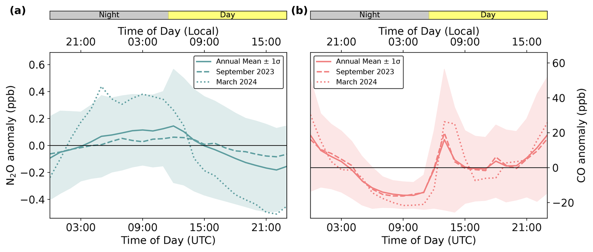
Figure 4 Observed diurnal cycle in (a) nitrous oxide (N₂O) and (b) carbon monoxide (CO) at GAL. The diurnal cycle is represented as the hourly anomaly from the daily mean mole fractions. Shading signifies 1-standard-deviation range for the overall mean. The solid black line represents zero anomaly. The time is reported in UTC to match the time zone used for reporting the mole fraction observation. The local time in the Galapagos is GMT−6. The color bar above each panel indicates daytime in yellow and nighttime in gray. No significant variation in day length is observed in the Galapagos due to its proximity to the Equator.

The N₂O diurnal cycle also varies seasonally between the dry and wet seasons. Compared to September 2023, March 2024 exhibits a larger diurnal variability, with an amplitude reaching 0.40 ppb. Additionally, the peak N₂O is observed earlier in the morning during the wet season compared to the annual mean. Despite the change in the N₂O diurnal-cycle amplitude seasonally, the diurnal cycles of temperature, wind speed, and relative humidity remain unchanged between the two seasons. However, the diurnal cycle of the wind direction has a larger amplitude in March 2024 compared to September 2023 (Fig. S6). A likely cause for this trend is the seasonal weakening of southeasterly winds over the Galapagos, allowing for more variable circulation, as illustrated in Fig. 5. Thus, the observed seasonal N₂O is mainly driven by the wind direction and the transport history of the air masses. It is important to note that the mean observed temperature in March 2024 (Fig. S6) is approximately 1 °C higher than the March climatology reported by Paltán et al. (2021), likely due to the El Niño event, lasting from June 2023 to May 2024. As a result, climatological seasonal differences may be less pronounced, and more years of observation are needed to draw a more definitive conclusion.

Compared to N₂O, the diurnal cycle of CO has a larger amplitude of 17.3 ppb, corresponding to 18 % of the background CO mole fractions. Unlike N₂O, CO has two peaks at 13:00 UTC (07:00 local time) and 00:00 UTC (18:00 local time). These peaks correspond to daily commuting hours and high tourism activity in Puerto Baquerizo Moreno and are likely due to increased anthropogenic emissions at these times. As the GAL station is located in the northern part of the population center with dominant southeasterly winds, the air masses are likely to accumulate such emissions. Nonetheless, a simultaneous increase in N₂O is not observed at these daily commuting hours, suggesting negligible local anthropogenic N₂O emissions. Additionally, no seasonal difference in the diurnal cycle is observed in CO despite the change in wind directions during the wet season, implying a minimal marine source and confirming the assumption that N₂O variability is dictated by air mass transport history, whereas CO conveys a signal of local combustion.

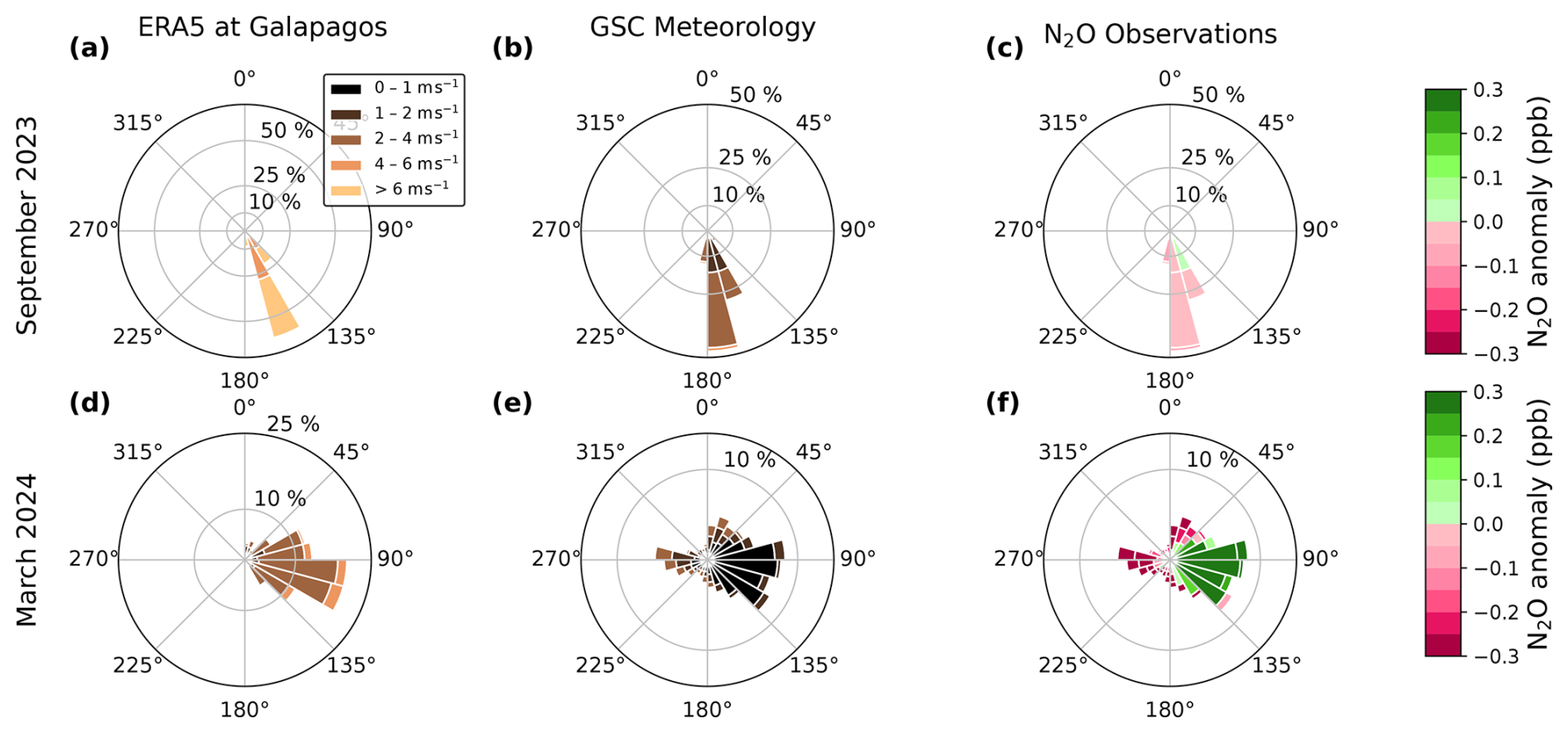
Figure 5 Observed vs. European Centre for Medium-Range Weather Forecasts (ECMWF) ERA5 surface wind speeds and directions in the Galapagos. Panels (a) and (d) show the monthly winds from ECMWF ERA5 for the grid cell where GAL is located (Hersbach et al., 2023). Panels (b) and (e) illustrate the winds observed at GAL, collected and reported by the Galapagos Science Center (GSC). Wind speed is indicated by the color bar, and the radial height of each bar represents the frequency of observations. Panels (c) and (f) show the mean nitrous oxide mole fraction anomaly from a 7 d running mean. The color bar indicates the mole fraction anomaly from a 7 d mean, and each bar's radial height represents the frequency of associated wind speed observations. Wind directions are represented by the angle of each bar around the polar axis. Panels (a)–(c) correspond to observations in September 2023, whereas panels (d)–(f) correspond to those in March 2024.

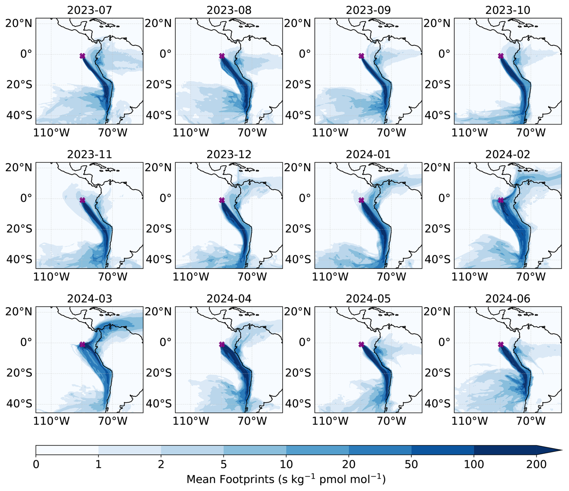
Figure 6 Monthly mean air mass back trajectory footprints simulated by the FLEXPART model and ERA5 reanalysis meteorology between July 2023 and June 2024. The footprints are derived from the total residence time of particles released at the Galapagos Emissions Monitoring Station in each grid cell at the surface (0–100 m) throughout 20 d back trajectories. The Galapagos Emissions Monitoring Station is marked with a purple X. Dates are formatted as YYYY-MM.

3.3 Seasonality and atmospheric circulation

The transport history of the air masses sampled at Galapagos is critical for understanding variability observed in N₂O mole fractions because the surface fluxes are distributed heterogeneously in space (Arevalo-Martínez et al., 2015; Buitenhuis et al., 2018; Nevison et al., 1995; Suntharalingam et al., 2000; Yang et al., 2020). The long atmospheric residence time of N₂O, 116 ± 9 years (Prather et al., 2015), and the lack of N₂O sinks in the troposphere (Tian et al., 2024) allow for lower-tropospheric N₂O mole fractions to be set solely by mixing or net surface exchange. Therefore, any variability in the N₂O is linked to either temporal variability in surface fluxes or the changes in the air mass transport history. As a regional product of wind speed and direction is required to generate such transport histories, i.e., footprints, we investigate the trends and variability in ERA5 and observed wind patterns over the Galapagos. We use the ECMWF ERA5 reanalysis product for the air mass footprint calculations as it assimilates various direct observations and forecast models to accurately represent the atmospheric circulation globally (Hersbach et al., 2023). Figure 3 illustrates that observed N₂O is higher during the wet season compared to during the dry season, with more substantial variability. To investigate the impact of seasonal changes in wind on the observed N₂O, we examined both observed and reanalysis wind data during the middle of each season (dry, September 2023; wet, March 2024) in Fig. 5. Local observations suggest that there is a shift from strong – on average, 2.01 ± 0.91 m s⁻¹ (1 SD) – southerly winds to weaker – on average, 0.67 ± 0.88 m s⁻¹ – easterly winds over the Galapagos. On the other hand, ERA5 reports higher wind speeds compared to direct observations, with a mean of 5.83 ± 0.89 m s⁻¹ in September 2023 and a mean of 2.62 ± 0.94 m s⁻¹ in March 2024. The difference is mainly justifiable because the ERA5 product estimates average winds over a 0.25° × 0.25° area at the surface. In contrast, the GSC observations are collected at a specific point within that grid cell. Similarly, wind directions between ERA5 and the GSC observations differ slightly, likely due to the impact of topography on the atmospheric circulation over the single observational point in a grid cell mainly dominated by an ocean surface. Nonetheless, the reanalysis product captures the seasonality in the winds, with a shift from strong southeasterly to weaker easterly winds, making the ERA5 product a suitable meteorological input for the atmospheric transport model discussed in Sect. 2.3.

Figure 5c and f suggest that there is no significant relationship between the N₂O mole fractions and the observed wind direction and speed during September due to a minor anomaly. On the other hand, the observed N₂O anomaly is correlated with the wind direction and speed during March. Due to the southward shift of the ITCZ to the latitude of the Galapagos in the eastern Pacific during the wet season, air masses are more stagnant over the Galapagos, which allows for the accumulation of some local N₂O emissions. This is evident as the easterly winds transporting air masses over the land contain more N₂O compared to air masses transported over the ocean via westerly winds. While the analysis of local winds could support the analysis of local impacts on the N₂O variability, they do not contain any information about the transport history of sampled air masses. Therefore, footprints calculated using the FLEXPART model are a better tool than the observed wind directions to examine the variability in the N₂O mole fraction anomalies as they represent the history of air masses over the different surfaces where emissions occur. Figure 6 shows the GAL's calculated air mass back trajectory footprints between July 2023 and June 2024, as described in Sect. 2.3. Between August and December, the air masses sampled at the station are dominantly transported over the western coast of South America, where intense marine N₂O fluxes have been reported (Arevalo-Martínez et al., 2015; Buitenhuis et al., 2018; Nevison et al., 1995; Suntharalingam et al., 2000; Yang et al., 2020). Additionally, most of the air masses enter the domain from the southern and southwestern boundaries, where air masses are likely to have low N₂O due to the lack of significant marine emissions in the central Pacific and Southern oceans (Buitenhuis et al., 2018; Thompson et al., 2014; Yang et al., 2020). Starting in December, air masses transported from the Northern Hemisphere are also sampled at the station, with the peak northern hemispheric influence in March 2024. Due to inter-hemispheric differences in N₂O mole fractions, more northern hemispheric influence in the later periods is likely to be the reason for the increased baseline between February and April 2024, setting the overall seasonal difference in N₂O.

3.4 Local nitrous oxide emissions

In addition to the seasonal and diurnal effects, the observed magnitude and variability of N₂O in the Galapagos can be attributed to the variability of fluxes over the eastern Pacific and South America. However, these analyses cannot account for local emissions in San Cristóbal, originating in the same grid cell as the sampling location. Therefore, independent estimates of local emissions are needed. Currently, there are only a limited number of studies estimating the greenhouse gas emissions from the Galapagos, and they are restricted to annual emissions (Mateus et al., 2023), reporting 6.2 metric tonnes of N₂O emissions annually, dominated by the marine transportation and aviation sectors. Even though 6.2 metric tonnes of N₂O emissions comprise <0.001 % of the estimated marine emissions from the eastern tropical Pacific (Yang et al., 2020), they can enhance N₂O mole fractions significantly if they are episodic and close to the measurement site. Thus, in Fig. 7, we explore three different indicators to determine potential N₂O enhancements associated with the local emissions close to the sampling location: (i) CO enhancement, (ii) wind stagnation, and (iii) a local regional influence metric (I_local).

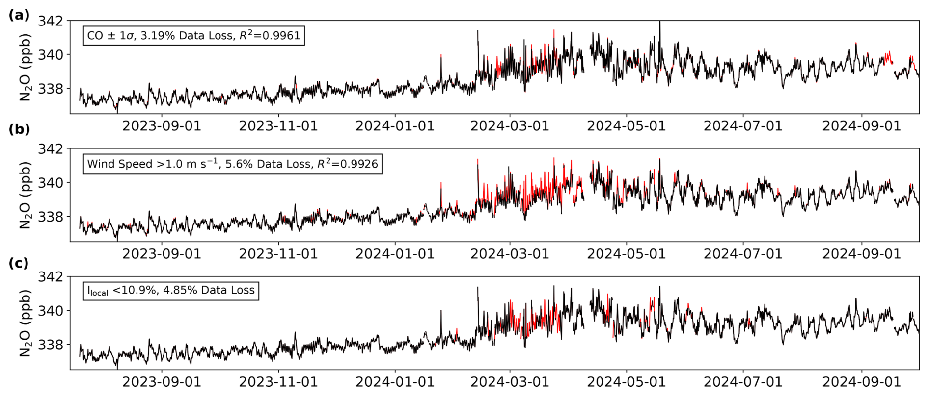
Figure 7 The 3-hourly averaged nitrous oxide mole fractions filtered based on (a) carbon monoxide mole fractions, (b) observed wind speed, and (c) the local regional influence metric (I_local). Filters are applied to the original 1 min average data. The black lines represent the nitrous oxide observations that satisfy the conditions described in the legend, whereas the red lines are the observations that are filtered out. Dates are formatted as YYYY-MM-DD.

Firstly, CO is an indicator of combustion activities associated with transportation, tourism, and energy generation as it is a by-product of combustion, similarly to N₂O (Cofer III et al., 1991; Watson et al., 1990), and any large-scale and episodic combustion events could simultaneously increase both N₂O and CO. To filter out such events, we use a 2-standard-deviation range around the monthly mean CO mole fraction. The filter rarely detects significant co-enhancement of N₂O and CO, and only a small portion, 3.19 %, of N₂O observations are filtered. Some 3-hourly averages are adjusted due to the filtering of individual observations, resulting in a pre-filter vs. post-filter R² value of 0.9961. Secondly, we use a wind speed filter based on the direct measurements at the GSC, assuming that slow wind speeds may allow longer residence times over the island and may accumulate more local emissions. Wind speeds below 1.0 m s⁻¹ are filtered out, resulting in a 5.6 % loss of 3-hourly average observations and a pre-filter vs. post-filter R² value of 0.9926. The filter mainly affects the N₂O enhancements between February and April 2024.

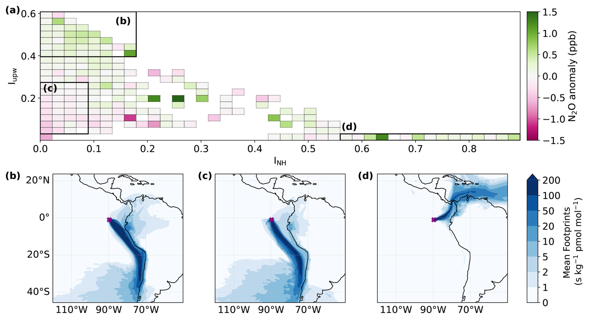
Figure 8 Attribution of observed nitrous oxide (N₂O) enhancements to air mass source regions, specifically the Peruvian and Chilean upwelling systems and the Northern Hemisphere. Panel (a) shows the mean anomaly of N₂O mole fractions relative to a 7 d mean, binned by varying levels of influence from upwelling systems (I_upw) and the Northern Hemisphere (I_NH). Definitions of the upwelling systems and Northern Hemisphere regions are provided in Fig. 2, and regional influences are calculated using Eq. (3). Mean footprint maps are shown under varying influences: (b) high upwelling, low Northern Hemisphere; (c) low upwelling, low Northern Hemisphere; (d) low upwelling, high Northern Hemisphere. Panel (a) shows bin ranges corresponding to panels (b)–(d).

Lastly, the local influence filter considers both the wind speed and direction to estimate how stagnant the air masses are close to the sampling site. The filter is defined by a 3 × 3 grid cell area centered on GAL as the local region and calculates the regional influence (I_local) following Eq. (3). The distribution of calculated I_local values is presented in Fig. S5. Due to the dominance of strong trade winds in the region throughout the observational period, the air masses are transported rapidly from the South American coast to the Galapagos. Therefore, the localness metric, I_local, is low, with a median of 4.4 % and a strong right-skewed distribution. Since 10.9 % represents the 95th percentile of I_local, we chose this critical value for filtering stagnant air masses with high local influence. Similar filtering of local effects based on transport model footprints is commonly implemented (An et al., 2024; Ganesan et al., 2015; Lunt et al., 2021; Saboya et al., 2024), with the specific critical value depending highly on the mean circulation and topography around the sampling sites. This filter removes 4.85 % of 3-hourly average N₂O mole fractions, mainly during late March and early April 2024. R² is arbitrary for this filter as the footprint calculations are only performed at 3 h intervals. Overall, all three filters mainly remove a small number of enhanced N₂O mole fractions during the wet season over the Galapagos. When combined, these filters suggest that the weakening and directional changes in the winds due to the seasonality of the ITCZ play a critical role in setting the time periods when local anthropogenic emissions might mask any regional marine emissions.

3.5 Nitrous oxide enhancements and marine emissions

After applying the three filters shown in Fig. 7 to exclude air masses potentially affected by local emissions, we examine the contribution of regional emissions from marine hotspots to the variability in observed N₂O. Given the strong oceanic fluxes from the Peruvian and Chilean upwelling systems in the eastern tropical Pacific (Arevalo-Martínez et al., 2015; Buitenhuis et al., 2018; Nevison et al., 1995; Suntharalingam et al., 2000; Yang et al., 2020), we calculate the upwelling influence (I_upw) as described in Sect. 2.3. The boundaries for the Peruvian and Chilean upwelling regions are defined based on Peru and Chile's exclusive economic zones and surface flux magnitudes following Yang et al. (2020) and are shown in Fig. 2. Similarly, we calculate the northern hemispheric influence (I_NH) to assess the impact of air mixing from the Northern Hemisphere on N₂O variability. The distributions of I_upw and I_NH throughout the observation period are provided in Fig. S5. The I_NH is low, with a median of 1.2 % and a strong right-skewed distribution because the transport of northern hemispheric air masses to the Galapagos is not common and is only limited to the wet season. On the other hand, I_upw is normally distributed, with a median of 30.0 %. Generally, air masses transported over the Peruvian upwelling system also pass over the Chilean upwelling system, as shown in Fig. 6 for October 2023. However, not all air masses that pass over the Chilean upwelling system travel over the Peruvian upwelling system. Given the similar mechanisms controlling fluxes in both regions, we combined the Peruvian and Chilean upwelling systems into a single region. This approach could mask the unique temporal variability and spatial extent of N₂O emissions from each upwelling system. While the grouped footprint influence metric is helpful in attributing variability to the heterogeneous spatiotemporal structure of marine fluxes, further attribution to each upwelling system is only possible with a future top-down inverse modeling study. To explore the role of these regional influences on N₂O variability, we compare their N₂O anomalies, calculated as a deviation from the 7 d running mean (Fig. 8).

From Fig. 8, we observe that air masses influenced by upwelling regions are generally associated with a significant positive N₂O anomaly relative to the 7 d mean. Air masses with high upwelling influence (I_upw>0.4) and low Northern Hemisphere influence (I_NH<0.18) exhibit a mean N₂O anomaly of 0.17 ± 0.36 ppb. These samples are predominantly transported over the Peruvian and Chilean upwelling zones, particularly near coastal regions where the most intense upwelling occurs (Fig. 8b). Although high I_upw correlates with more positive N₂O anomalies, the observed standard deviation exceeds twice the mean value, suggesting that variability in surface fluxes may significantly influence N₂O fluctuations in addition to atmospheric transport effects.

In contrast, air masses with I_upw<0.09 and I_NH<0.27 display a mean N₂O anomaly of −0.17 ± 0.27 ppb, indicating that these air masses, largely transported by southeasterly winds over the eastern tropical Pacific Ocean, remain offshore from the high N₂O emission zones within the Peruvian and northern Chilean upwelling systems (Fig. 8c). The extent of the upwelling region and the magnitude of associated fluxes likely play a critical role in determining the mean N₂O levels in this low upwelling system and low northern hemispheric influence regime. The large standard deviation around this mean may be attributed to spatial variability that deviates from the defined boundaries of the upwelling systems, as outlined by Yang et al. (2020). For instance, the extent and intensity of N₂O fluxes can be significantly altered during the El Niño events due to a more stratified surface ocean in the eastern Pacific. Thus, while synoptic-scale N₂O variability is modulated by air mass transport pathways driven by winds, spatial heterogeneity in marine fluxes along the upwelling zones is essential for capturing the observed variability. Lastly, air masses with I_upw<0.03 and I_NH>0.56 show a mean N₂O anomaly of 0.20 ± 0.52 ppb. These air masses with negligibly low upwelling system influence and high northern hemispheric influence do not overlap with any significant oceanic N₂O sources; however, emissions from northwestern South America and southern Central America could play a role in modifying the N₂O anomaly based on the footprint distribution (Fig. 8d). Additionally, increased N₂O in the Northern Hemisphere compared to the Southern Hemisphere (Prinn et al., 2018) could result in higher observed N₂O at the Galapagos during periods of high northern hemispheric influence.

4 Conclusions

This study addresses a significant gap in long-term monitoring of atmospheric N₂O content in the eastern tropical South Pacific, a region strongly influenced by substantial marine N₂O emissions and climate variability modes like ENSO. We presented continuous, high-frequency N₂O and CO measurements collected at the Galapagos Emissions Monitoring Station from July 2023 to September 2024, located in San Cristóbal, Galapagos Islands, Ecuador. Our findings highlight that N₂O variability in this region is strongly driven by seasonal trade winds, which regulate air mass mixing between the Northern Hemisphere and the Southern Hemisphere and the air mass transport over marine nitrous oxide hotspots. During the wet season, we observed elevated variability in N₂O and CO due to reduced wind speeds that allowed local pollution to accumulate before reaching the sampling site. By implementing filters based on CO measurements, wind speed, and air mass transport models, we minimized the potential influence of these local pollution events, ensuring an accurate representation of regional N₂O trends. A comparison of diurnal cycles further suggests that local anthropogenic emissions do not impact N₂O variability, except for a limited number of pollution events during the wet season. Prominently, during the dry season, air masses with high influence from the Peruvian and Chilean upwelling systems exhibited elevated N₂O levels at GAL, linking marine N₂O emissions to atmospheric concentrations at this site. Additionally, the analysis of regional influences clarified that the spatial and temporal variability in surface N₂O emissions could strongly modify the observed N₂O, underscoring the heterogeneity of fluxes in the eastern Pacific and the need for continued continuous measurements. While this study provides valuable insights, the current methods cannot provide more robust estimates of marine and terrestrial fluxes in the region. Follow-up studies with inverse modeling approaches are needed to further dissect the impacts of spatial and temporal heterogeneity on atmospheric N₂O variability in this region.