A CO₂–Δ¹⁴CO₂ inversion setup for estimating European fossil CO₂ emissions

Independent estimation and verification of fossil CO₂ emissions on a regional and national scale are crucial for evaluating the fossil CO₂ emissions and reductions reported by countries as part of their nationally determined contributions (NDCs). Top-down methods, such as the assimilation of in situ and satellite observations of different tracers (e.g., CO₂, CO, Δ¹⁴CO₂, XCO₂), have been increasingly used for this purpose. In this paper, we use the Lund University Modular Inversion Algorithm (LUMIA) to estimate fossil CO₂ emissions and natural fluxes by simultaneously inverting in situ synthetic observations of CO₂ and Δ¹⁴CO₂ over Europe. We evaluate the inversion system by conducting a series of observing system simulation experiments (OSSEs). We find that in regions with a dense sampling network, such as western/central Europe, adding Δ¹⁴CO₂ observations in an experiment where the prior fossil CO₂ and biosphere fluxes are set to zero allows LUMIA to recover the time series of both categories. This reduces the prior-to-truth root mean square error (RMSE) from 1.26 to 0.12 TgC d⁻¹ in fossil CO₂ and from 0.97 to 0.17 TgC d⁻¹ in biosphere fluxes, reflecting the true total CO₂ budget by 91 %. In a second set of experiments using realistic prior fluxes, we find that in addition to retrieving the time series of the optimized fluxes, we are able to recover the true regional fossil CO₂ budget in western/central Europe by 95 % and in Germany by 97 %. In all experiments, regions with low sampling coverage, such as southern Europe and the British Isles, show poorly resolved posterior fossil CO₂ emissions. Although the posterior biosphere fluxes in these regions follow the seasonal patterns of the true fluxes, a significant bias remains, making it impossible to close the total CO₂ budget. We find that the prior uncertainty of fossil CO₂ emissions does not significantly impact the posterior estimates, showing similar results in regions with good sampling coverage like western/central Europe and northern Europe. Finally, having a good prior estimate of the terrestrial isotopic disequilibrium is important to avoid introducing additional noise into the posterior fossil CO₂ fluxes.

1 Introduction

Carbon dioxide (CO₂) from fossil fuels and cement production has become the dominant source of anthropogenic emissions to the atmosphere since around 1950, leading to a mixing ratio of CO₂ in the atmosphere of 419.70 ppm on 16 September 2023, which is 49 % above pre-industrial levels (https://gml.noaa.gov/ccgg/trends/gl_trend.html, last access: 18 September 2023). Although land and ocean sinks of CO₂ have increased over the past 6 decades, the fraction of emissions removed from the atmosphere is expected to decline as the CO₂ mixing ratio increases; therefore, a higher proportion of emitted CO₂ will remain in the atmosphere (Eyring et al., 2021). Monitoring CO₂ emissions and removals is important to follow compliance with international treaties such as the Paris Agreement (UNFCCC, 2016). In the agreement, the parties have committed to report their emissions and removals of CO₂ and other greenhouse gases (GHGs) to the United Nations Framework Convention on Climate Change (UNFCCC) through the annual GHG inventory. In the case of fossil CO₂ emissions, these inventories have been reported to have uncertainties between 5 % and 10 % in developed countries. These annual inventories and other national-level data are used to spatially and temporally distribute CO₂ emissions at sub-national and sub-annual scales. These spatially distributed products help us to better understand the sources of CO₂ emissions and to implement more effective policies toward emission reduction (Han et al., 2020). Commonly available emission products, such as the Carbon Dioxide Information and Analysis Center (CDIAC) FFCO₂ emission maps (Andres et al., 2011), the Open-source Data Inventory for Anthropogenic CO₂ (ODIAC) emission data product (Oda and Maksyutov, 2011; Oda et al., 2018), and the Emissions Database for Global Atmospheric Research (EDGAR) (Janssens-Maenhout et al., 2019), use national energy statistics, power plant emission data, and spatial proxies such as nighttime light observations, population data, and road transport networks to spatially and temporally distribute the emissions. This additional information introduces new uncertainties that, in EDGAR, for instance, can reach a global uncertainty of approximately 11 % (Solazzo et al., 2021) or can be as high as 120 % in the case of CDIAC (Andres et al., 2016). These uncertainties can be more significant and challenging to characterize at sub-annual and sub-national scales, even in developed countries (Basu et al., 2016; Miller et al., 2012).

These emission products can be used alongside atmospheric observations of CO₂ and other tracers in inverse modeling systems to reduce their uncertainty, enhance our understanding of fossil CO₂ emissions and natural fluxes, and improve the accuracy of national carbon budgets. So far, atmospheric CO₂ inversion frameworks have predominantly been used to constrain terrestrial sources and sinks of CO₂ (Basu et al., 2013; Chevallier et al., 2007; Monteil et al., 2020; Monteil and Scholze, 2021). To constrain the terrestrial carbon cycle, inverse modelers typically prescribe fossil CO₂ fluxes from emission data products, like those mentioned previously, assuming them to be perfectly well-known (Turnbull et al., 2009). Atmospheric CO₂ represents a mixture of all sources, with the natural signal being predominant during most of the year (the growing season covers spring to fall), masking the contribution of fossil CO₂ emissions (Shiga et al., 2014). Consequently, additional information is necessary to segregate the fossil contribution from the natural signal in atmospheric CO₂ observations to constrain the fossil CO₂ fluxes. Some strategies have included sampling approaches where observations are taken close to major fossil CO₂ sources (e.g., cities and power plants) (Bréon et al., 2015) or satellite observations of large point sources such as column-integrated atmospheric CO₂ mixing ratios (XCO₂) (Kaminski et al., 2022; Wang et al., 2020). A more commonly employed method is to combine these CO₂-only observations (either CO₂ or XCO₂) with additional tracers such as NO₂ and the NO_x:CO₂ ratio (Kuhlmann et al., 2021) or ground observations of CO (Newman et al., 2013; Brioude et al., 2013), APO (atmospheric potential oxygen) (Pickers et al., 2022), and, more widely, the radiocarbon (Δ¹⁴CO₂) content of carbon dioxide (Turnbull et al., 2009; Basu et al., 2016; Wang et al., 2018), which we use in this study.

Radiocarbon is the radioactive isotope of carbon with a half-life of approximately 5730 years and is produced naturally in the upper atmosphere by cosmic-ray-induced reactions with nitrogen (Turnbull et al., 2009). Fossil CO₂ does not contain radiocarbon (it has already decayed), and adding its ¹⁴C-free emissions to the atmosphere causes a depletion of Δ¹⁴CO₂ (Suess, 1955). Meanwhile, radiocarbon is being absorbed and released by the ocean and the biosphere, making it an effective tracer of the natural carbon cycle and, therefore, a tool to distinguish fossil emissions from the natural cycle signal in atmospheric CO₂ observations (Turnbull et al., 2009, 2022; Zazzeri et al., 2023). Radiocarbon is also produced as a by-product of nuclear facilities (e.g., nuclear power plants) and atmospheric nuclear weapon tests, the latter occurring mostly between 1945 and 1980, with the highest intensity in 1961–1962 (Naegler and Levin, 2006). These bomb tests caused a significant disturbance in the radiocarbon cycle, resulting in an isotopic disequilibrium in the biosphere and ocean (Hesshaimer et al., 1994). Isotopic disequilibrium is the difference between the isotopic signatures or radiocarbon content of carbon entering and leaving a pool. Despite its similar meaning, this occurs differently in the ocean and the biosphere. In the ocean, the disequilibrium results from Δ¹⁴C-depleted CO₂ from water that has returned to the surface and was out of contact with the atmosphere, allowing the radiocarbon to decay significantly. In the biosphere, the disequilibrium is a result of the heterotrophic respiration of Δ¹⁴C-enriched CO₂ assimilated a couple of decades ago when the atmospheric Δ¹⁴C was higher due to the bomb spike (Lehman et al., 2013). Therefore, the ocean disequilibrium flux tends to dilute the atmospheric Δ¹⁴C content, whereas the biosphere disequilibrium flux tends to enrich it.

The usefulness of atmospheric Δ¹⁴CO₂ observations in estimating the fossil CO₂ content in the atmosphere as a fraction of the total atmospheric CO₂ mixing ratio has been demonstrated in various modeling studies. For instance, Levin and Karstens (2007) present an observational approach to estimate hourly regional fossil fuel CO₂ offsets at a continental site (Heidelberg, Germany) using weekly mean ¹⁴CO₂-based fossil fuel CO₂ mixing ratios and CO observations. On a larger scale, Levin et al. (2008) examine monthly mean ¹⁴CO₂ observations from two German stations (Schauinsland and Heidelberg), compared against background measurements from Jungfraujoch, to assess the regional fossil fuel CO₂ surplus and emphasize the importance of high-precision radiocarbon measurements for quantifying fossil fuel CO₂ contributions at a regional scale in Europe. The study by Miller et al. (2012) explores the relationship between fossil fuel CO₂ emissions and enhancements in atmospheric mixing ratios of ¹⁴CO₂ and other anthropogenic trace gases. Utilizing a 6-year dataset from vertical profiles in the northeastern US, they separate the fossil and natural components of atmospheric CO₂ using apparent emission ratios of various gases to fossil fuel CO₂, offering observation-based estimates of national emissions and comparing these with inventory-based estimates. Turnbull et al. (2015) use measurements of CO₂, ¹⁴CO₂, and CO from multiple sampling towers around Indianapolis (Indiana, US) to differentiate fossil fuel CO₂ from background levels in an urban environment and evaluate the consistency of a bottom-up emission product. More recently, by using radiocarbon observations in CH₄ (Δ¹⁴CH₄) and CO₂ (Δ¹⁴CO₂) over London, Zazzeri et al. (2023) reveal that fossil fractions of CH₄ and atmospheric mixing ratios of fossil CO₂ are consistently higher than those predicted by simulations using emission products such as EDGAR. This discrepancy highlights the potential of ¹⁴CO₂ measurements to refine our understanding of fossil and biospheric CO₂ and CH₄ partitioning in urban settings, especially when the influence of nuclear power plants is minimal.

Nevertheless, large-scale four-dimensional inversion systems have only recently begun to include Δ¹⁴CO₂ as an additional tracer to constrain fossil CO₂ emissions. Basu et al. (2016) introduced a novel dual-tracer atmospheric inversion technique that differentiates between biospheric and fossil fuel CO₂ fluxes using atmospheric CO₂ and Δ¹⁴CO₂ measurements over the US. This method not only allows for the estimation of monthly regional fossil fuel CO₂ fluxes but also addresses biases in biospheric flux estimates that occur when using traditional CO₂-only inversion methods with fixed fossil fuel flux assumptions. Their approach represents a significant advancement in quantifying regional and national fossil fuel emissions from atmospheric observations. Building upon this study, Basu et al. (2020) presented a more focused analysis in providing national and sub-national-scale estimates of fossil fuel CO₂ emissions using an extensive observation database of both CO₂ and Δ¹⁴CO₂. Graven et al. (2018) conducted an in-depth analysis of fossil fuel CO₂ emissions in California, utilizing atmospheric observations from nine sites and employing the Weather Research and Forecasting model along with the Stochastic Time-Inverted Lagrangian Transport model (WRF-STILT). The research integrates measurements of CO₂ mixing ratio and Δ¹⁴CO₂, uniquely combining these observations with high-resolution emission data from Vulcan v2.2 and EDGARv4.2, aiming to refine estimates of regional fossil fuel CO₂ emissions and explore the impact of various factors such as nuclear industry emissions and air–sea exchanges on atmospheric CO₂ levels. In Europe, Wang et al. (2018) evaluated the potential of a Δ¹⁴CO₂ observation network for estimating regional fossil fuel CO₂ emissions through atmospheric inversions. They examined the effectiveness of different network configurations, from minimal to very dense setups, in reducing uncertainties in fossil CO₂ emissions estimations. The study used synthetic observations and the LMDZv4 global transport model, paying special attention to representation and aggregation errors. Establishing a network of both CO₂ and Δ¹⁴CO₂ measurement stations requires significant investments to ensure long monitoring periods that allow the identification of sub-annual- and sub-national-scale variations in fossil CO₂ emissions. The Integrated Carbon Observation System (ICOS) atmospheric network includes 39 stations in 14 European countries and overseas territories. Hourly CO₂ atmospheric observations are available for 26 stations, with the earliest data from 2015 when the network was established. However, some of these stations already existed by then, and there is information from previous years. A total of 14 stations measure Δ¹⁴CO₂ in 2-week integrated samples analyzed by the ICOS Central Radiocarbon Laboratory. The ICOS network is expanding to include more stations, and new sampling strategies are being developed to increase the number of Δ¹⁴CO₂ measurements.

In this work, we present the new capabilities of the Lund University Modular Inversion Algorithm (LUMIA) system (Monteil and Scholze, 2021) to perform simultaneous inversions of atmospheric CO₂ and Δ¹⁴CO₂ observations as a first attempt to develop a model capable of supporting the monitoring and verification of fossil CO₂ emissions across Europe. Such emissions monitoring and verification support capacities are essential for assessing compliance with international agreements, such as the Paris Agreement (UNFCCC, 2016), and for guiding policy decisions aimed at reducing carbon emissions, as described by Janssens-Maenhout et al. (2020). We perform observing system simulation experiments (OSSEs), recreating the current state of the ICOS network and its sampling strategy and using different flux products (as priors and true values) to demonstrate the performance of the inversion scheme and show its capabilities. We begin by assessing the impact of oceanic fluxes on the total mixing ratios of CO₂ and Δ¹⁴CO₂. Then, we evaluate the impact of adding Δ¹⁴CO₂ observations on the estimation of fossil CO₂ emissions by comparing the model's ability to recover true fluxes starting from a prior flux set to zero. Finally, with a more realistic setup, i.e., prior, we evaluate the impact of the prescribed fossil CO₂ flux uncertainty and the impact of the terrestrial isotopic disequilibrium product.

2 Theoretical background

The depletion of radiocarbon in the atmosphere due to fossil CO₂ emissions has been demonstrated in various studies since the 1950s, primarily through the Δ¹⁴C content of tree rings (Suess, 1955; Tans et al., 1979). Anthropogenic disturbances in atmospheric radiocarbon content, such as those from nuclear bomb tests and nuclear power facilities (Hesshaimer and Levin, 2000), have led to a deeper understanding of the radiocarbon exchange processes between the atmosphere, the biosphere (Hahn et al., 2006), and the ocean (Hesshaimer et al., 1994).

With subsequent advances in measurement and modeling techniques, Δ¹⁴CO₂ observations have been used to estimate the fossil CO₂ offset within atmospheric CO₂ mixing ratios (Levin and Hesshaimer, 2000; Kuc et al., 2003; Naegler and Levin, 2006; Levin and Karstens, 2007; Levin et al., 2008). This is achieved by comparing observations from free-troposphere background stations with those from regionally polluted stations, establishing an essential foundation for estimating fossil CO₂ emissions using inverse modeling, as will be discussed in the following sections.

2.1 Regional transport model

We use the LUMIA (Lund University Modular Inversion Algorithm) system as described by Monteil and Scholze (2021), modifying the way background mixing ratios (y^b in Eq. 1) are calculated by computing a smoothed and detrended average of real observations from the ICOS network for each sampling site. Originally, the LUMIA system was developed to optimize regional net ecosystem exchange (NEE) fluxes over Europe using in situ CO₂ observations from the ICOS (Integrated Carbon Observation System) Atmosphere network. In this study, we have extended LUMIA to additionally assimilate Δ¹⁴CO₂ observations from the same network and optimize multiple flux categories. This extension introduces a new step in the mass balance of atmospheric transport as follows:

$$\begin{array}{}\text{(1a)}& {\displaystyle }{y}_{{\mathrm{CO}}_{\mathrm{2}}}=y_{{\mathrm{CO}}_{\mathrm{2}}}^{\mathrm{b}}+\sum _{c}K\left({\mathit{F}}_c\right),\text{(1b)}& {\displaystyle }{y}_{\mathrm{C}{\mathrm{\Delta }}^{\mathrm{14}}\mathrm{C}}=y_{\mathrm{C}{\mathrm{\Delta }}^{\mathrm{14}}\mathrm{C}}^{\mathrm{b}}+\sum _{c}K\left({\mathbf{\Delta }}_c{\mathit{F}}_c\right),\end{array}$$

where $y_{{\mathrm{CO}}_{\mathrm{2}}}$ and $y_{\mathrm{C}{\mathrm{\Delta }}^{\mathrm{14}}\mathrm{C}}$ represent the modeled mixing ratios of CO₂ and CΔ¹⁴C, respectively, and $y_{{\mathrm{CO}}_{\mathrm{2}}}^{\mathrm{b}}$ and $y_{\mathrm{C}{\mathrm{\Delta }}^{\mathrm{14}}\mathrm{C}}^{\mathrm{b}}$ denote their background mixing ratios (i.e., the boundary condition), derived from smoothed real observations (see Sect. 3.3). Since the values of Δ¹⁴CO₂ in per mill (‰) units are not additive (as it represents the change of the ¹⁴C:¹²C atmospheric ratio relative to an absolute standard of ¹⁴C from 1950; Stuiver and Polach, 1977), we convert all Δ¹⁴CO₂ values to values of CO₂ × Δ¹⁴CO₂ (or CΔ¹⁴C for simplification) (Basu et al., 2016). In terms of units, for mixing ratios this would be CΔ¹⁴C ppm ‰ and for fluxes PgC ‰ yr⁻¹. Since per mill (‰) only means multiplication by 1000, we drop that factor from Δ¹⁴C into the quantity CΔ¹⁴C, expressing it in parts per million (ppm) for mole fractions and PgC yr⁻¹ for fluxes to maintain the same order of magnitude and units for CO₂ and CΔ¹⁴C. For example, a sample with a CO₂ mole fraction of 400 ppm and a Δ¹⁴C value of 45 ‰ would have CΔ¹⁴C = 18 ppm. Expressed in this way, CΔ¹⁴C becomes additive and can be transported by a model.

The operator K represents the regional transport model (pre-computed footprints; see Sect. 3.2), which is used to calculate the contribution of surface fluxes F (in each category c) to the change of CO₂ and CΔ¹⁴C in the atmosphere. F_c in this study corresponds to gridded fluxes with a resolution of 0.5° × 0.5° and 1 h. In Eq. (1b), the term Δ_c represents the fraction of ¹⁴C in the accompanying flux category F_c (Tans et al., 1979; Turnbull et al., 2016).

Expanding the foreground (regional) part of Eq. (1) to include the flux categories explicitly yields

$$\begin{array}{}\text{(2a)}& \sum _{c}K\left({\mathit{F}}_c\right)=K\left({\mathit{F}}_{\mathrm{ff}}\right)+K\left({\mathit{F}}_{\mathrm{bio}}\right)+K\left({\mathit{F}}_{\mathrm{oce}}\right),\end{array}$$

where F_ff is the fossil CO₂ emission, F_bio is the net CO₂ flux between the atmosphere and terrestrial ecosystems (net ecosystem exchange, NEE, hereafter also called biosphere flux), and F_oce is the atmosphere–ocean CO₂ exchange. Calculating each K(F_c) separately tracks the influence of each category, not just the total. For radiocarbon, the equation looks similar but includes an additional term for the radiocarbon from nuclear facilities.

$$\begin{array}{}\text{(2b)}& {\displaystyle }\begin{array}{rl}& \sum _{c}K\left({\mathbf{\Delta }}_c{\mathit{F}}_c\right)\\ & =K\left({\mathbf{\Delta }}_{\mathrm{ff}}{\mathit{F}}_{\mathrm{ff}}\right)+K\left({\mathbf{\Delta }}_{\mathrm{atm}}\left({\mathit{F}}_{\mathrm{bio}}+{\mathit{F}}_{\mathrm{oce}}\right)\right)\\ & +K\left(\left({\mathbf{\Delta }}_{\mathrm{bio}}-{\mathbf{\Delta }}_{\mathrm{atm}}\right){\mathit{F}}_{\mathrm{bio}\mathrm{2}\mathrm{atm}}\right)\\ & +K\left(\left({\mathbf{\Delta }}_{\mathrm{oce}}-{\mathbf{\Delta }}_{\mathrm{atm}}\right){\mathit{F}}_{\mathrm{oce}\mathrm{2}\mathrm{atm}}\right)+K\left({\mathbf{\Delta }}_{\mathrm{nuc}}{\mathit{F}}_{\mathrm{nuc}}\right)\end{array}\text{(2c)}& {\displaystyle }\begin{array}{rl}& =K\left({\mathbf{\Delta }}_{\mathrm{ff}}{\mathit{F}}_{\mathrm{ff}}\right)+K\left({\mathbf{\Delta }}_{\mathrm{atm}}\left({\mathit{F}}_{\mathrm{bio}}+{\mathit{F}}_{\mathrm{oce}}\right)\right)+K\left({\mathit{F}}_{\mathrm{biodis}}\right)\\ & +K\left({\mathit{F}}_{\mathrm{ocedis}}\right)+K\left({\mathbf{\Delta }}_{\mathrm{nuc}}{\mathit{F}}_{\mathrm{nuc}}\right)\end{array}\end{array}$$

Here, Δ_ff is set equal to −1000 ‰, indicating that the fossil CO₂ does not contain any Δ¹⁴CO₂ and therefore dilutes the atmospheric Δ¹⁴CO₂ content. Δ_atmF_bio and Δ_atmF_oce refer to the exchange of “modern” CΔ¹⁴C between terrestrial ecosystems and the ocean, respectively, with the atmosphere, since Δ¹⁴C in new biomass and the top layer of the ocean would almost match atmospheric Δ¹⁴C (Δ_atm) (Graven et al., 2020). F_biodis and F_ocedis represent the isotopic disequilibrium, or the isotopic difference between the source (ocean or biosphere) and the atmosphere. F_biodis is “old-captured” and Δ¹⁴C-enriched CΔ¹⁴C released by heterotrophic respiration (F_bio2atm). F_ocedis is old-captured and Δ¹⁴C-depleted CΔ¹⁴C released through vertical transport of water masses (F_oce2atm) (Lehman et al., 2013; Basu et al., 2016). F_nuc is the radiocarbon production due to nuclear activities, mainly from nuclear facilities, since radiocarbon production from nuclear bomb tests has stopped largely (Hesshaimer and Levin, 2000). Converting Δ_nucF_nuc to CΔ¹⁴C notation, for modeling purposes, as mentioned above, is achieved through

$$\begin{array}{}\text{(3)}& {\mathbf{\Delta }}_{\mathrm{nuc}}{\mathit{F}}_{\mathrm{nuc}}={\displaystyle \frac{N}{r_{\mathrm{std}}}}{\mathit{F}}_{\mathrm{nuc}},\end{array}$$

where r_std is the standard ¹⁴C:C ratio ($\mathrm{1.176}\times {\mathrm{10}}^{-\mathrm{12}}$), and $N=(\mathrm{975}/({\mathit{\delta }}^{\mathrm{13}}\mathrm{C}+\mathrm{1000}){)}^{\mathrm{2}}$ is the isotope fractionation correction (Stuiver and Polach, 1977). As the δ¹³C value, we use the global atmospheric yearly average of −8 ‰ (Basu et al., 2016). Combining Eqs. (1) through (3) for the modeled CO₂ and Δ¹⁴CO₂ mixing ratios, yields the following:

$$\begin{array}{}\text{(4a)}& {\displaystyle }{y}_{{\mathrm{CO}}_{\mathrm{2}}}=y_{{\mathrm{CO}}_{\mathrm{2}}}^{\mathrm{b}}+K\left({\mathit{F}}_{\mathrm{ff}}\right)+K\left({\mathit{F}}_{\mathrm{bio}}\right)+K\left({\mathit{F}}_{\mathrm{oce}}\right)\text{(4b)}& {\displaystyle }\begin{array}{rl}{y}_{\mathrm{C}{\mathrm{\Delta }}^{\mathrm{14}}\mathrm{C}}& =y_{\mathrm{C}{\mathrm{\Delta }}^{\mathrm{14}}\mathrm{C}}^{\mathrm{b}}+K\left({\mathbf{\Delta }}_{\mathrm{ff}}{\mathit{F}}_{\mathrm{ff}}\right)+K\left({\mathit{F}}_{\mathrm{biodis}}\right)\\ & +K\left({\mathit{F}}_{\mathrm{ocedis}}\right)+K\left({\mathbf{\Delta }}_{\mathrm{atm}}\left({\mathit{F}}_{\mathrm{bio}}+{\mathit{F}}_{\mathrm{oce}}\right)\right)\\ & +K\left({\displaystyle \frac{N}{r_{\mathrm{std}}}}{\mathit{F}}_{\mathrm{nuc}}\right)\end{array}\end{array}$$

An additional source of radiocarbon, cosmogenic production, occurs naturally in the upper atmosphere as a result of cosmic-ray-induced reactions with nitrogen. This term is implicitly included in the background $y_{\mathrm{C}{\mathrm{\Delta }}^{\mathrm{14}}\mathrm{C}}^{\mathrm{b}}$.

2.2 Observations

We perform inversions for a regional domain ranging from 15° W, 33° N to 35° E, 73° N, as shown in Fig. 1. This domain is consistent with those used in previous studies, such as Monteil et al. (2020) and Thompson et al. (2020). The sampling stations depicted in Fig. 1 represent the ICOS Atmosphere network for the years 2018–2020, noting that new sampling stations have been added since that period. The ICOS Atmosphere network is a component of ICOS, a European research infrastructure designed to provide long-term, high-quality, and harmonized observations of carbon dynamics. The network includes 33 stations across Europe, all measuring CO₂, with 15 of these stations also measuring Δ¹⁴CO₂.

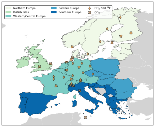
Figure 1 Study domain and location of the ICOS Atmosphere network sampling stations used in this paper. The regions will be used for the analysis and discussion of the results.

There are two sampling strategies used at the ICOS stations: continuous sampling and periodic sampling. Continuous sampling is performed at almost every available sampling height at the station using commercially available automatic samplers for hourly measurements of, for example, CO₂. Periodical sampling, on the other hand, is conducted only at the highest sampling height using flask samplers. These flasks are later analyzed in various ICOS laboratories. Hourly integrated flask samples, collected every 3 d, serve both as quality control for continuous sampling and for measuring other gases not continuously monitored (e.g., SF₆, H₂, stable isotopes of CO₂), in addition to Δ¹⁴CO₂ for the determination of the atmospheric fossil CO₂ component through inverse modeling (Levin et al., 2020). Furthermore, a 2-week integrated flask sample is designed to pass air over an NaOH solution, specifically for Δ¹⁴CO₂ sampling.

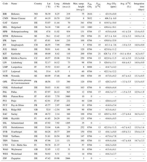
In this paper, we use the continuous 1 h CO₂ and integrated 2-week Δ¹⁴CO₂ periodic sampling strategies for the evaluation of LUMIA. A summary of the stations, including their location, sampling height, number and average of measurements, and integration days, is presented in Table 1.

Table 1 Observation stations used in this study. Included is a summary of the number of observations (N_obs), the average observations ± 1 standard deviation, and the integration time of Δ¹⁴CO₂ samples for the year 2018 based on data accessible through the ICOS Python API (https://pypi.org/project/icoscp/, last access: 7 January 2025). Stations with zero N_obs did not measure or report observations of the corresponding tracer in 2018 to ICOS but are incorporated into this study for a comprehensive analysis.

2.3 Inverse modeling problem

Atmospheric inverse modeling can be used for a variety of purposes, including the establishment of the initial conditions of a model, the identification of sources and sinks, and the evaluation and improvement of prior emissions (Bocquet et al., 2015). The goal is to estimate the best set of variables (fluxes) consistent with atmospheric measurements of a tracer (e.g., CO₂ and Δ¹⁴CO₂) in the study domain (observations), given the atmospheric transport that relates the two. In its most basic form, this can be formulated as

$$\begin{array}{}\text{(5a)}& \mathit{y}=H\left(\mathit{x},\mathit{b}\right)+\mathit{\epsilon },\end{array}$$

where the control vector x contains the variables to be estimated and the observation vector y contains the observations (atmospheric mixing ratios). H is the observation operator, which includes the transport model and any additional processing of observations, such as accounting for the boundary conditions and variables b, which we will not optimize. ε is the error vector that includes the errors in the observations, the transport model, and the control vector. By pre-subtracting the prior model estimate for the observations, y^apri, Eq. (5a) can be rewritten as $\mathit{y}={\mathit{y}}^{\mathrm{apri}}+H\left(\mathit{x}\right)+\mathit{\epsilon }$, with y^apri the a priori model estimate for the observations, computed following Eq. (4). In this case, Eq. (5a) can be simplified as

$$\begin{array}{}\text{(5b)}& {\mathit{\delta }}_{\mathit{y}}=\mathbf{H}\mathit{x}+\mathit{\epsilon },\end{array}$$

where ${\mathit{\delta }}_{\mathit{y}}=\mathit{y}-{\mathit{y}}^{\mathrm{apri}}$ is the vector storing the prior model–data mismatches. In our case, the atmospheric transport is linear; thus, H(x) can be rewritten as Hx, where H is the Jacobian of H (Monteil and Scholze, 2021).

There are multiple approaches to solving the inverse modeling problem. In this paper, and in general in LUMIA, we use the variational approach, in which the control vector x that minimizes the cost function in Eq. (6) is sought iteratively by minimizing the mismatch between the model outputs and the observations (Chatterjee and Michalak, 2013; Rayner et al., 2019; Scholze et al., 2017):

$$\begin{array}{}\text{(6)}& \begin{array}{rl}J\left(\mathit{x}\right)& ={\displaystyle \frac{\mathrm{1}}{\mathrm{2}}}{\left(\mathit{x}-{\mathit{x}}^{\mathrm{b}}\right)}^T{\mathbf{B}}^{-\mathrm{1}}\left(\mathit{x}-{\mathit{x}}^{\mathrm{b}}\right)\\ & +{\displaystyle \frac{\mathrm{1}}{\mathrm{2}}}{\left(\mathbf{H}\mathit{x}-{\mathit{\delta }}_{\mathit{y}}\right)}^T{\mathbf{R}}^{-\mathrm{1}}\left(\mathbf{H}\mathit{x}-{\mathit{\delta }}_{\mathit{y}}\right),\end{array}\end{array}$$

where B is the prior uncertainty covariance matrix, and R is the observational uncertainty covariance matrix (defined as a diagonal matrix) controlling the weight of each observation in the model–data mismatch δ_y and the target variable (x^b) in the optimization. The iterative procedure searches for the value of x that minimizes J(x) – that is, the value of x for which the gradient (∇_xJ) is equal to zero. To reduce the number of iterations and large matrix multiplications, the optimization is performed on a preconditioned control vector $\mathit{\omega }={\mathbf{B}}^{-\mathrm{1}/\mathrm{2}}(\mathit{x}-{\mathit{x}}^{\mathrm{b}})$. More information on preconditioning can be found in Monteil and Scholze (2021).

2.3.1 Construction of the control vector (x)

The control vector x contains the set of parameters adjustable by the inversion, which are offsets to the different sources and sinks of CO₂ and Δ¹⁴CO₂ that we want to estimate. From Eq. (4), our main interest is to optimize the fossil CO₂ flux F_ff. However, since through the radiocarbon cycle, we can separate fossil and biogenic CO₂, we also need to optimize the fluxes from the biosphere (F_bio), as well as the isotopic disequilibrium F_biodis, to reduce the uncertainty of these two terms, which can have an important impact on the inversion result. The remaining fluxes (F_nuc, F_oce, and F_ocedis) are prescribed.

To limit the computational requirements, we do not solve directly for the high-resolution fluxes (e.g., 0.5° × 0.5° and 1-hourly) used in the transport model but for weekly offsets for 2500 clusters of grid cells. Appendix B describes the clustering algorithm in more detail, and the script can be found in lumia/Tools/optimization_tools.py of the LUMIA source code provided as an asset. In short, it groups contiguous grid cells, depending on how sensitive the observation network is to their emissions: grid cells directly upwind of the sampling stations are optimized at the native resolution of 0.5°, but in parts of the domain not well-sampled by the observations (e.g., North Africa, Türkiye), the resolution drops down to 5° × 3.5° (see Fig. 2).

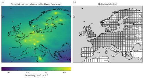
Figure 2 Visual representation of (a) the sensitivity of the observation network to each grid cell (in logarithmic scale) and (b) the optimized clusters and their variable spatial resolution.

Equation (5b) can be rewritten as

$$\begin{array}{}\text{(7)}& {\mathit{\delta }}_{\mathit{y}}=\sum _c\mathbf{H}{\mathit{x}}_c,\end{array}$$

where H is the Jacobian matrix of the observation operator with dimensions $(n_{\mathrm{obs}},n_{p_{\mathrm{opt}}}\times n_{t_{\mathrm{opt}}})$, and x_c, with dimensions $(n_{p_{\mathrm{opt}}}\times n_{t_{\mathrm{opt}}})$, represents the portion of the control vector x that contains offsets for the optimized categories c. Thus, x_c is built from the relative contribution of each model time step t_mod (1 h) and of each grid cell p_mod (0.5° × 0.5°) to each optimized time step t_opt and cluster p_mod. Here, $n_{t_{\mathrm{opt}}}$ and $n_{p_{\mathrm{opt}}}$ represent the number of optimized intervals (weekly) and grid cell clusters (e.g., 2500 for the biosphere), respectively.

2.3.2 Construction of the prior error covariance matrix (B)

Our matrix B is constructed such that we first determine the spatiotemporal structure of the uncertainties, which is then scaled to match the reported uncertainties. Since we optimize for offsets, the prior control vector x^b contains only zeros (so ${\mathbf{F}}_c={\mathbf{F}}_c^{\mathrm{0}}$). The uncertainties in x^b are given by the error covariance matrix B. We assume no correlation between different categories and different tracers. Therefore, sections of B specific to each tracer or category can be constructed independently. We do this in three steps.

1. Construct a vector of variances (diagonals of B), which contain the spatiotemporal pattern of the uncertainties.

2. Construct the covariances based on spatial and temporal correlation functions. Specifically, the covariances are set following $\text{cov}({\mathit{x}}_i,{\mathit{x}}_j)={\mathit{\sigma }}_{{\mathit{x}}_i}{\mathit{\sigma }}_{{\mathit{x}}_j}{e}^{-{\left(d(p_i,p_j)/L_{\mathrm{h}}\right)}^{\mathrm{2}}}{e}^{-|t_i-t_j|/L_{\mathrm{t}}}$, with d(p_i,p_j) the great circle distance between the center of the clusters (area-weighted average of the center coordinates of the grid cells in the cluster) and $|t_j-t_i|$ the temporal distance between x_i and x_j. i and j refer to the position in the control vector with assigned space and time coordinates; i.e., x_i has coordinates (p_i, t_i), and x_j has coordinates (p_j, t_j). L_h and L_t represent the horizontal and temporal correlation lengths, respectively.

3. Scale the entire (section of the) B matrix by a uniform scaling factor to match a prescribed category-specific annual uncertainty value δF_c.

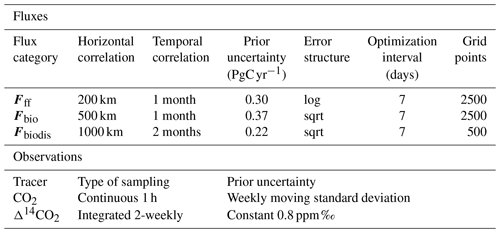
The values of the correlation lengths L_h and L_t, as well as the scaling factors δF_c, are provided in Sect. 3.4. For constructing the vector of variances (${\mathit{\sigma }}_x^{\mathrm{2}}$), two approaches were used.

• For fossil CO₂ emissions F_ff, the variance is set to ${\mathit{\sigma }}_{p,t,c}^{\mathrm{2}}=|{\sum }_{i,j,t_{\mathrm{mod}}}{\mathit{F}}_{i,j,t_{\mathrm{mod}}}^c{|}^{\mathrm{2}}$, where ${\mathit{\sigma }}_{p,t,c}^{\mathrm{2}}$ is the variance corresponding to the control vector elements for the interval t and spatial cluster p of category c. The spatial coordinates i and j are the ensemble of grid cells that are within the cluster p, and the temporal coordinate t_mod is the ensemble of 1-hourly model time steps that are within the (weekly) optimization interval t. For instance, if the cluster p groups four model grid cells, the variance ${\mathit{\sigma }}_{p,t,c}^{\mathrm{2}}$ will be calculated over 672 flux components (four grid cells, 7 d with 24-hourly time steps).

• For the other fluxes, the procedure is similar, but the formula is ${\mathit{\sigma }}_{p,t,c}^{\mathrm{2}}=\sqrt{\left|{\sum }_{i,j,t_{\mathrm{mod}}}{\mathit{F}}_{i,j,t_{\mathrm{mod}}}^c\right|}$.

The rationale behind these formulas is to scale the uncertainties to the prior estimate of the fluxes (assuming that very low prior fluxes should imply low prior uncertainties) but avoid artificially low errors in instances where negative and positive fluxes compensate for each other (i.e., NEE in the spring and autumn). Furthermore, the location of fossil CO₂ emissions is relatively better known. Therefore, the formula used for fossil CO₂ emissions concentrates the uncertainties more at the location of prior emissions than that used for the other categories. Regardless of the formula used for determining the variance, it is scaled afterward to match the target uncertainty reported in Table 2.

Table 2 Parameter setup used in all the inversions performed in this study.

3 Observing system simulation experiments (OSSEs)

To assess the performance of the inversion system, we designed and performed a series of perfect transport observing system simulation experiments (hereafter called OSSEs). In OSSEs, the impact of new observing systems, existing system configurations, observing strategies, and new data optimization on the quantification of the target variables is evaluated (Hoffman and Atlas, 2016). This is done by generating a set of simulated observations, called synthetic observations, from a set of reasonable but arbitrary fluxes, ${\mathit{F}}_c^{\mathrm{t}}$, considered “true” fluxes in the OSSE. Then, by using fluxes from different models or products as prior fluxes (F_c), we investigate the ability of an inverse modeling system to reconstruct the true fluxes consistent with the model setup (e.g., prescribed uncertainties, error structure), making assumptions such as perfect transport and perfect boundary conditions. Since they totally neglect the systematic model and representation errors, which should be accounted for in a real inversion, perfect transport OSSEs lead to overly optimistic results and should be interpreted with care. They are, however, well-suited to our objective here, which is to test the robustness of our implementation of the dual-tracer inversion. In the following sections, we describe the different datasets, model setups, assumptions, and experiments used in this study.

3.1 True and prior fluxes

We use a set of fluxes commonly used in this kind of inverse problem with a high horizontal and temporal resolution (0.5° × 0.5° and 1 h, respectively) to generate our synthetic observations. For the CO₂ fluxes, we use the EDGARv4.3 emission database (Janssens-Maenhout et al., 2019) distributed spatially and temporally based on fuel type, category, and country-specific emissions, using the COFFEE approach (Steinbach et al., 2011) (EDGAR in Table 3; see Gerbig and Koch, 2021b) as ${\mathit{F}}_{\mathrm{ff}}^{\mathrm{t}}$ for the base year 2018. For ${\mathit{F}}_{\mathrm{bio}}^{\mathrm{t}}$, we use a simulation of the LPJ-GUESS vegetation model (Smith et al., 2014) (LPJ-GUESS in Table 3; see Wu, 2023), and for ${\mathit{F}}_{\mathrm{oce}}^{\mathrm{t}}$, we use the Jena CarboScope v1.5 product (Rödenbeck et al., 2013). We use the terrestrial and ocean disequilibrium and nuclear fluxes from Basu et al. (2020) as our ${\mathit{F}}_{\mathrm{biodis}}^{\mathrm{t}}$ (BASU in Table 3), ${\mathit{F}}_{\mathrm{ocedis}}^{\mathrm{t}}$, and ${\mathit{F}}_{\mathrm{nuc}}^{\mathrm{t}}$, respectively.

As prior fluxes, we use products that follow different methodologies and schemes, with different spatial and temporal structures than the true fluxes, to make the implementation more realistic. For F_ff, we use a version of ODIAC (Open-source Data Inventory for Anthropogenic CO₂) (ODIAC in Table 3; see Oda and Maksyutov, 2020) with a 1 km × 1 km spatial and monthly temporal resolution. Thus, our prior fossil CO₂ fluxes include monthly variability but do not resolve the daily cycle (Oda et al., 2018). We also prepare a flat-year average version of this product (FlatODIAC in Table 3). For F_bio, we use a product from simulations of the VPRM vegetation model (Mahadevan et al., 2008; Thompson et al., 2020) (VPRM in Table 3; see Gerbig and Koch, 2021a). Due to the lack of an alternative product for F_biodis, we generate our own prior by calculating a series of randomly perturbed versions of the true flux following their prescribed uncertainties and their horizontal and temporal correlations (RndBASU in Table 3). This perturbation is done by adding a random perturbation to the control vector and transforming such a vector to the flux space. All fluxes are gridded to 0.5° × 0.5° and 1 h resolution by nearest-neighbor interpolation.

3.2 Observation footprints (FLEXPART)

Similar to Monteil and Scholze (2021), we compute the regional transport (e.g., operator H in Eq. 4) using the FLEXPART 10.4 Lagrangian transport model (Pisso et al., 2019). For each observation, FLEXPART computes a “footprint”, i.e., a vector containing the sensitivity of the observation to changes in the surface fluxes. The footprints are pre-computed and then used throughout the subsequent steps of the inversion (see Monteil and Scholze, 2021, for further details). The FLEXPART simulations were driven by ERA5 reanalysis data at a horizontal resolution of 0.5° × 0.5° and 1-hourly temporal resolution (Hersbach et al., 2018). The footprints were computed differently for the CO₂ and Δ¹⁴CO₂ observations. For CO₂, we computed a set of footprints for each observation up to 14 d backward in time, following the approach from Monteil and Scholze (2021). Integrated Δ¹⁴CO₂ observations (Sect. 2.2) quantify the Δ¹⁴C value of atmospheric CO₂ throughout 1 to 3 weeks (see Table 1). We account for this in FLEXPART by distributing the FLEXPART particles released over the whole integration period of the observations. The simulations are then carried out for (up to) 14 d backward in time from the start of the integration period. A Python code was developed to run FLEXPART and post-process the footprints being used in LUMIA (https://github.com/lumia-dev/runflex, last access: 7 January 2025). In Fig. 3, we show an example of an observation footprint for CO₂ and Δ¹⁴CO₂ at the Hyltemossa ICOS station in southern Sweden. The CO₂ footprint (Fig. 3a) shows how the observation for 26 June 2018 at 13:00 LT is sensitive to fluxes from the North Atlantic, passing through Norway and Sweden and finally from Sweden's east and south coasts close to the Baltic Sea. The Δ¹⁴CO₂ aggregated footprint, on the other hand, shows more spread sensitivity due to the long integration time, collecting fluxes from southern Norway, northwestern Europe, and the Baltic.

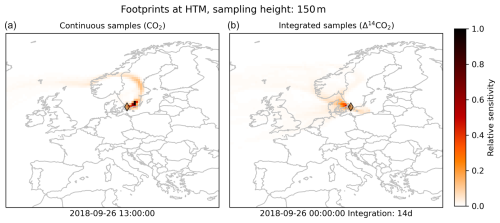
Figure 3 Examples of so-called (pre-calculated) footprints for CO₂ (a) and Δ¹⁴CO₂ (b) at the Hyltemossa ICOS station. The maps show the sensitivity of the respective atmospheric tracer at the sampling site to the surface fluxes over the regional domain up to 2 weeks before the observation. Panel (a) displays the sensitivity of CO₂ at the indicated sampling time and shows influences by surface fluxes from the North Atlantic through Scandinavia, while panel (b) demonstrates the dispersed sensitivity of a 14 d integrated Δ¹⁴CO₂ sample across northwestern Europe and the Baltic region. The two maps illustrate the distinct spatial integration of the two tracers over time.

3.3 Synthetic observations and background mixing ratios

We generate mixing ratio time series for 1 year for each of the stations according to the current setup of the ICOS Atmosphere network as described in Sect. 2.2. For replicating the most realistic conditions of the sampling frequency, we use real sampling and integration times (in the case of radiocarbon) from the stations, taking for each one the sampling times for 2018. In this way, we account for the sampling gaps and the differences in integration times commonly produced due to maintenance and general operational eventualities. For stations with the number of observations, N_obs, equal to zero in Table 1, we set fixed sampling and integration times (14 d). Most of these stations were already in operation in 2018, but some were not yet labeled as ICOS stations (e.g., Schauinsland) or had not implemented and or started the tracer measurement (e.g., Δ¹⁴CO₂ at Ochsenkopf).

Following Monteil and Scholze (2021), we select the CO₂ observation times according to the sampling station's elevation to guarantee the model's best representation. For sampling stations located under 1000 m a.s.l, we select the times when the boundary layer is most likely well-developed, from 11:00 to 15:00 LT. For the contrary case, we take the times around midnight, from 22:00 to 02:00 LT, when the boundary layer is most likely below the sampling intake or, in other words, is sampling the free troposphere. For our OSSEs, we use the same transport model (i.e., the pre-computed observation footprints from FLEXPART) to generate the synthetic observations and perform the inversions. Therefore, this data selection is not strictly necessary for this study, but we want to replicate the conditions of a real inversion. Since we are using the same background mixing ratio for the synthetic observations and the simulated prior and posterior observations (i.e., we are assuming a perfect boundary condition), we simplify the calculation of it by computing a smoothed and detrended weekly (for CO₂) and monthly (for Δ¹⁴CO₂) average of the real observations (ICOS et al., 2023) for each sampling site. For sampling sites for which there are for some reason no real observations for the year 2018 in the ICOS database (e.g., Δ¹⁴CO₂ measurements were not yet implemented or were not yet part of ICOS), we took the observations from the nearest year available to calculate the background.

We then perform a forward run of the model using the true fluxes mentioned in Sect. 3.1 to calculate the corresponding “true” CO₂ and Δ¹⁴CO₂ mixing ratio time series and add the background value corresponding to each site, observation time, and tracer. To weaken the assumption of a perfect transport and boundary condition, we add a random perturbation to the synthetic observations. This random perturbation is equal to ${\mathit{y}}^{{\mathrm{so}}^{*}}={\mathit{y}}^{\mathrm{so}}+\mathit{\epsilon }\times \mathit{\xi }$, where y is the synthetic observation, ε is the observation error (both the instrumental and representativity errors; see Sect. 3.4 below), and ξ is a standard normal random vector. In this way, the added perturbation is based on the observation error. Figure 4 shows the synthetic CO₂ and Δ¹⁴CO₂ observation time series and the components of each flux at the Hyltemossa station. As mentioned in Sect. 2.1, we convert all radiocarbon values to CΔ¹⁴C values. For the observation, we do this by applying the following equation:

$$\begin{array}{}\text{(8)}& \left[\mathrm{C}{\mathrm{\Delta }}^{\mathrm{14}}\mathrm{C}\right]={\displaystyle \frac{\left[{\mathrm{\Delta }}^{\mathrm{14}}{\mathrm{CO}}_{\mathrm{2}}\right]\times \left[{\mathrm{CO}}_{\mathrm{2}}\right]}{\mathrm{1000}}}.\end{array}$$

In a real setup, this would imply having paired CO₂ and Δ¹⁴CO₂ observations, and in the case of the integrated samples, this would mean having an average of CO₂ observations along the integration period of the Δ¹⁴CO₂ sample. However, since we are using synthetic observations, we transported the CO₂ fluxes using the Δ¹⁴CO₂ footprints and stored the values to convert back and forth between Δ¹⁴CO₂ and CΔ¹⁴C units (‰ and ppm, respectively).

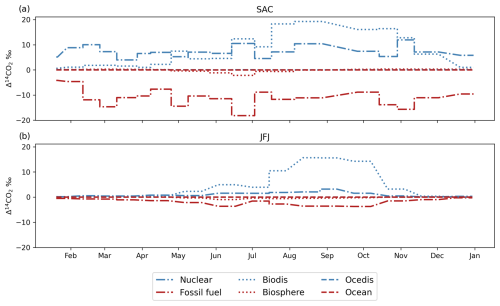
As can be seen from Fig. 4, both ${\mathit{F}}_{\mathrm{oce}}^{\mathrm{t}}$ and ${\mathit{F}}_{\mathrm{ocedis}}^{\mathrm{t}}$ have virtually no impact on the mixing ratios at the Hyltemossa station (and all other stations used in our setup; not shown), and hence we decided not to include these components in the control vector; i.e., we transport them but do not optimize them further.

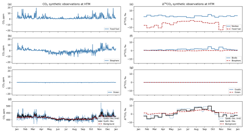
Figure 4 Synthetic observations of CO₂ and Δ¹⁴CO₂ at the HTM station over a 1-year period. Panels (a) to (d) display CO₂ mixing ratio variations due to different sources: (a) fossil fuel, (b) biosphere, (c) ocean, and (d) combined synthetic observations with random perturbation (dotted blue line) against the background mixing ratios (dashed red line). Panels (e) to (h) illustrate Δ¹⁴CO₂ variations: (e) nuclear and fossil fuel, (f) biospheric disequilibrium and biosphere, (g) ocean disequilibrium and ocean, and (h) total synthetic observations with random perturbation (dotted blue line) compared to the background (dashed red line). The solid and dashed blue lines represent the synthetic observations without and with random noise added, respectively.

3.4 Experiments and inversion setup

To make the inversions comparable, we keep the same inversion setup for all the experiments. Table 2 summarizes the main model parameter values. We choose a Gaussian horizontal correlation and an exponential temporal correlation for the prior flux uncertainties (see Sect. 2.3.1). Since our main purpose in this study is to demonstrate that our multi-tracer inversion system is capable of estimating both the fossil CO₂ emissions and natural CO₂ fluxes, we choose prior uncertainty values that are reasonable and consistent with other studies. The prior uncertainties are assigned as follows: for F_ff, we use the difference between the annual budgets for the whole study domain from ODIAC (1.26 PgC yr⁻¹) (Oda and Maksyutov, 2020) and from an emissions product based on EDGARv4.3 (1.47 PgC yr⁻¹) (Gerbig and Koch, 2021b) as a reference to define its uncertainty (Basu et al., 2016). We use 150 % (0.3 PgC yr⁻¹) of the difference as the base uncertainty for all the experiments, and we select two extra values to evaluate the impact of the prescribed uncertainty on the inversion: 50 % of the difference (0.1 PgC yr⁻¹) and the exact difference of 0.21 PgC yr⁻¹ (100 %). For F_bio we choose 25 % (0.37 PgC yr⁻¹) of the monthly prior (Monteil and Scholze, 2021) and 30 % (0.22 PgC yr⁻¹) of the annual budget for F_biodis (Basu et al., 2020). We optimize all the categories at the same temporal resolution but at a higher horizontal resolution for F_ff and F_bio (2500 points) than for F_biodis (500 points). To set up the observation error, which includes the instrumental and the representativity errors, we use different methods for the CO₂ and the Δ¹⁴CO₂. For CO₂, where the error of representativity is usually larger than the instrumental error, we apply a weekly moving standard deviation to each observation; i.e., the prior error of each observation is equal to the standard deviation of the observations in a time window of ±3.5 d around that observation. In this way, we account for the changes in the CO₂ mixing ratios according to the local site conditions. For instance, at a background station such as Jungfraujoch (JFJ) at the top of the Swiss Alps, the observation error ranges from 0.9 to 29.2 ppm (mean value of 9.3 ± 4.0 ppm), while at polluted sites such as Saclay (SAC) just outside Paris, the CO₂ mixing ratios change rapidly and the error ranges from 5.9 to 215.5 ppm (mean value of 55.8 ± 40.7 ppm). For Δ¹⁴CO₂, on the other hand, the instrumental error is larger than the representativity error, and we use a constant value of 0.8 ppm in CΔ¹⁴C units or 1.91 ± 0.05 ‰ in Δ¹⁴CO₂ units, calculated using Eq. (8).

We perform one forward run and six inversions, summarized in Table 3. We generate the synthetic observations and evaluate the impact of ${\mathit{F}}_{\mathrm{oce}}^{\mathrm{t}}$ and ${\mathit{F}}_{\mathrm{ocedis}}^{\mathrm{t}}$ on the total synthetic observations as described in Sect. 3.3 with the forward run (SYNTH). Starting with the inversions, we perform two experiments to test the impact of having Δ¹⁴C observations (ZBASE and ZCO2Only). We use the prior F_ff and F_bio set to zero (in both the spatial and temporal domain) with a prior uncertainty setup based on ODIAC and VPRM, respectively. The reason for using prior fluxes set to zero is that the flux products for both categories can have spatial and temporal distributions similar to their respective true values, making it easier for the model to retrieve the true fluxes. Instead, we set the values to zero but give the model some information through the prior uncertainty setup. The remaining fluxes are prescribed and set to their true values. We assimilate both CO₂ and Δ¹⁴C observations for ZBASE and only CO₂ observations for ZCO2Only. In the second set of inversions, we use a more realistic setup. In the first, BASE, we simulate a complete and realistic inversion setup, assimilating CO₂ and Δ¹⁴C observations and optimizing F_ff, F_bio, and F_biodis. In the BASE experiments, we change the prescribed prior uncertainty of F_ff (0.1, 0.21 and 0.3 PgC yr⁻¹) to evaluate its impact on the optimization.

In the final inversion, BASENoBD, we prescribe F_biodis (i.e., the true value in this context) instead of optimizing it. The terrestrial disequilibrium term (F_biodis) is challenging to estimate due to the large uncertainties associated with heterotrophic respiration fluxes and the age of respired carbon (Basu et al., 2016). These uncertainties can vary significantly depending on the vegetation model or methodology used. We compare the posterior F_ff of this experiment with the one of the BASE experiment (in which F_biodis is optimized) to evaluate the impact of the prior F_biodis product on the posterior F_ff. By keeping F_biodis fixed in BASENoBD, we can assess how much of the error in the posterior F_ff of BASE comes from the additional optimization of F_biodis.

Table 3 Inversions performed in this work.

4 Results

4.1 Impact of F_oce and F_ocedis

We start by testing the impact of ocean-related fluxes (${\mathit{F}}_{\mathrm{oce}}^{\mathrm{t}}$ and ${\mathit{F}}_{\mathrm{ocedis}}^{\mathrm{t}}$) in the total synthetic observations by performing a forward simulation (SYNTH in Table 3). Figure 4 shows the results from this forward simulation and the contribution of each flux category to the mixing ratios of both tracers for the Hyltemossa (HTM) station. The results show that the contribution of the ocean and ocean disequilibrium fluxes to the total mixing ratio is below the error assigned to the synthetic observations. For CO₂, the average contribution is −0.07 ± 0.12 ppm (for an average observation error of 10.0 ± 5.7 ppm) at HTM and −0.07 ± 0.15 ppm (average obs. error 9.8 ± 9.0 CO₂ ppm) at all stations. For Δ¹⁴CO₂, the average contribution due to F_oce is −0.009 ± 0.009 ‰ (average obs. error 1.9 ± 0.04 ‰) at HTM and −0.007 ± 0.007 ‰ (average obs. error 1.9 ± 0.05 ‰) at all stations. Similarly, the contribution due to F_ocedis is 0.016 ± 0.009 ‰ at HTM and 0.02 ± 0.017 ‰ at all stations. Due to the low impact of ocean-related fluxes, we prescribe them in the inversions along with F_nuc and optimize only F_ff, F_bio, and F_biodis. A summary for each station can be found in Appendix A.

4.2 Impact of adding Δ¹⁴CO₂ observations

In this section, we present the results from the ZBASE and ZCO2Only experiments. We start by analyzing the retrieval of truth fossil CO₂ (${\mathit{F}}_{\mathrm{ff}}^{\mathrm{t}}$) and biosphere (${\mathit{F}}_{\mathrm{bio}}^{\mathrm{t}}$) time series. We divide the results into the regions shown in Fig. 1, where northern Europe represents Scandinavia, Finland, and the Baltic States; western/central Europe represents Benelux, France, Germany, Switzerland, Liechtenstein, and Austria; southern Europe represents the Iberian Peninsula, Italy, and the Balkans (except for Romania and Bulgaria); eastern Europe represents Poland, Slovakia, Hungary, Romania, and Bulgaria; and the British Isles represent Ireland and the United Kingdom. The study domain includes all the land shown in Fig. 1, even the countries not mentioned in the definition of the regions (countries in gray in Fig. 1).

4.2.1 Retrieval of the monthly and regional time series

In general, there is closer agreement between the posterior and the truth for the biosphere fluxes (F_bio) than for the fossil CO₂ emissions (F_ff) in both the ZBASE and ZCO2Only experiments. This means that the model performs better at recovering F_bio from the observations compared to F_ff, as shown in Fig. 6 for F_bio and Fig. 5 for F_ff. In the study domain, the inclusion of Δ¹⁴CO₂ observations in the ZBASE experiment yields better performance than ZCO2Only for both flux categories. Specifically, the posterior F_ff ZBASE exhibits closer alignment with the truth than ZCO2Only with a lower RMSE (see Table 4), indicating a better fit of the seasonality for F_ff. Similarly, the posterior biosphere fluxes more closely follow the true time series than the fossil CO₂ emissions in both experiments, with ZBASE outperforming ZCO2Only in terms of RMSE and bias values.

The regional analysis reflects the influence of the coverage by sampling stations on the inversion outcomes. Western/central Europe, benefiting from the highest number of stations (18 out of 33 stations considered in this study, 10 of them measuring both tracers), shows the best alignment between the posterior and true time series for F_ff, especially in the ZBASE experiment (Fig. 5b), while ZCO2Only shows pronounced RMSE and bias values (Table 4). Conversely, regions like eastern Europe (one station measuring both tracers) and the British Isles (two stations measuring only CO₂), despite their lower station coverage, exhibit posterior ZBASE F_ff time series that closely approximate the truth, with eastern Europe showing consistent performance throughout the year (Fig. 5d and f). However, the posterior ZBASE biosphere fluxes in these regions do not align as closely with the true values as observed in, e.g., western/central Europe (Fig. 6d and f). In eastern Europe, the posterior ZBASE shows big differences from the truth during May, June (maximum difference of 0.42 TgC d⁻¹), and later in September, while ZCO2Only shows a better fit during these months but a positive bias the rest of the year (Fig. 6d). In contrast, the posterior biosphere flux from the ZCO2Only experiment shows a better fit to the truth than the ZBASE one in the British Isles (Table 4).

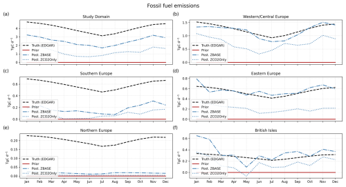
Figure 5 Monthly fossil CO₂ truth (dashed lines), prior (solid lines), and posterior fluxes from the ZBASE (dashed–dotted lines) and ZCO2Only (dotted lines) experiments for (a) the study domain and the five sub-regions defined: (b) western/central Europe, (c) southern Europe, (d) eastern Europe, (e) northern Europe, and (f) the British Isles.

Table 4 RMSE and bias values for F_ff and F_bio from the ZBASE and ZCO2Only experiments in all the regions.

Lastly, southern Europe and northern Europe show similar results despite their differences: northern Europe has better coverage of sampling stations, and its annual truth fossil CO₂ emissions are lower (an average of 0.20 TgC d⁻¹ against 0.59 TgC d⁻¹). In both regions, the posterior F_ff of the two experiments is far from the truth (Fig. 5c and e), while the posterior F_bio values of both regions and experiments are close to each other, with northern Europe showing a better fit to the truth than southern Europe, in which the posterior shows a more pronounced positive bias along the year (Fig. 6c and e).

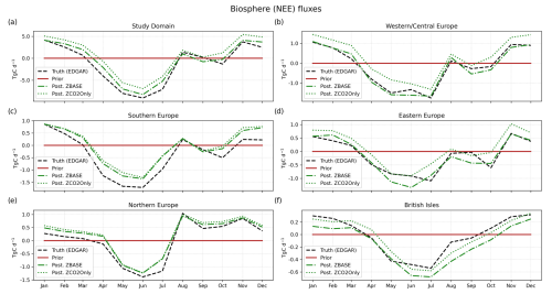
Figure 6 Monthly biosphere (NEE) truth (dashed lines), prior (solid lines), and posterior fluxes from the ZBASE (dashed–dotted lines) and ZCO2Only (dotted lines) experiments for (a) the study domain and the five sub-regions defined: (b) western/central Europe, (c) southern Europe, (d) eastern Europe, (e) northern Europe, and (f) the British Isles.

4.2.2 Analysis of the spatial error reduction

We set up the ZBASE and ZCO2Only experiments with prior uncertainties and error structures as in Table 2 based on the values of ODIAC for F_ff and VPRM for F_bio. Therefore, the model had some information about the spatial and temporal error structure of the prior fluxes. To evaluate the spatial performance of LUMIA, we first aggregate the hourly values (both truth and posterior) to the optimization interval of 1 week. After this, we calculate the posterior RMSE of each experiment and flux category at the grid cell level, and finally, we calculate the RMSE reduction by subtracting the posterior RMSE of ZBASE from the posterior RMSE of ZCO2Only as follows.

$$\begin{array}{}\text{(9)}& {\text{RMSE}}_{\mathrm{reduction}}={\text{RMSE}}_{\mathrm{ZCO}\mathrm{2}\mathrm{Only}}^{\mathrm{apos}}-{\text{RMSE}}_{\mathrm{ZBASE}}^{\mathrm{apos}}\end{array}$$

Here, positive values of RMSE_reduction indicate posterior RMSE${}_{\mathrm{ZBASE}}^{\mathrm{apos}}$ values that are lower than RMSE${}_{\mathrm{ZCO}\mathrm{2}\mathrm{Only}}^{\mathrm{apos}}$, i.e., grid cells where when adding Δ¹⁴C observations (ZBASE) shows values closer to the truth (better performance, lower RMSE) than when only having CO₂ observations (ZCO2Only). For fossil fuel, we find larger prior RMSE values in western/central Europe, but some grid cells also show the location of larger cities like in southern England, Poland, and Spain (Fig. 7a). For the biosphere fluxes, we find larger prior RMSE values in western/central Europe and the British Isles (Fig. 7e).

The largest positive RMSE reductions (where ZBASE performs better than ZCO2Only) (Fig. 7d and h) occur around the sampling stations in western/central Europe and the British Isles for both flux categories. For fossil CO₂, most of the study domain has positive values (92 %), although a large number of these values (around 75 %) are close to zero, representing the values in southern and northern Europe where there is a low adjustment of the fluxes when adding Δ¹⁴C observations (Fig. 7d). For the biosphere fluxes, the posterior RMSE maps (Fig. 7f and g) show the regions that are poorly constrained due to the absence of observations such as the southern part of the domain and the Baltic States. Despite a lower portion of the study domain (40 %) (Fig. 7h) showing an improvement in the posterior estimation when adding Δ¹⁴C observations compared with fossil fuel, this presents a clearer pattern in areas such as southeastern England, the northern part of western/central Europe, Denmark, and southern Sweden, as well as some areas in eastern Europe.

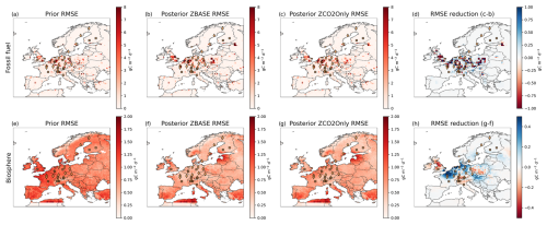
Figure 7 Spatial error of fossil CO₂ (a–d) and the biosphere (e–h) for the ZBASE and ZCO2Only experiments. Panels (a) and (e) show the prior RMSE for F_ff and F_bio, respectively; panels (b) and (f) show the posterior RMSE for ZBASE; panels (c) and (g) show the posterior RMSE for ZCO2Only; and panels (d) and (h) show the RMSE reduction (see Eq. 9) for fossil CO₂ and the biosphere. In panels (d) and (h), positive values (in blue) show the pixels where ZBASE performs better than ZCO2Only (i.e., adding Δ¹⁴CO₂ observations improves the posterior estimates), and negative values (in red) show where ZCO2Only performs better than ZBASE. Crosses and diamonds represent stations that only measure CO₂ and those that additionally measure Δ¹⁴CO₂, respectively.

4.2.3 Recovery of the annual budget

Next, we assess how accurately the model can estimate the annual budget for fossil fuel, biosphere (NEE), and total CO₂. Figure 8 shows the annual budget of the study domain, the sub-regions (right), and some of the largest European countries by area (left). We include the ODIAC emission data product and the VPRM product for the biosphere in Fig. 8 as references since we base the prior uncertainty and error structure on the spatial and temporal distribution of these two products. As we find in the temporal distribution (Fig. 5), in the study domain, the posterior fossil CO₂ from both experiments does not fit the truth, but ZBASE shows a lower bias from the truth than ZCO2Only. This result is reflected in the annual budget, where ZBASE recovers 63 % from ${\mathit{F}}_{\mathrm{ff}}^{\mathrm{t}}$, while ZCO2Only recovers only 32 % (Fig. 8a). Likewise, the posterior F_bio of ZBASE that closely fits ${\mathit{F}}_{\mathrm{bio}}^{\mathrm{t}}$ recovers 38 % of the biosphere budget (Fig. 8b), while ZCO2Only, which shows a larger positive bias in the temporal distribution, returns a positive annual budget, contrary to the negative annual budget of the true biosphere fluxes. This behavior is repeated in most of the regions and countries shown in Fig. 8, where ZCO2Only strongly underestimates the annual fossil CO₂ emissions, with the lowest estimates in southern (15 %) and northern Europe (2 %) – the latter with a strong underestimation from ZBASE as well (9 %) – France (33 %), and Spain (∼ 0 %), which has a similar situation as northern Europe (5 % recovery for ZBASE) and returns an annual biosphere budget that compensates for the total CO₂ budget that is close to ZBASE in most of the cases.

Western Europe and eastern Europe show the best posterior F_ff ZBASE values of 95 % and 105 % of the truth, respectively. However, while some countries in these regions with good sampling coverage, such as the Benelux Union, show good recovery of ${\mathit{F}}_{\mathrm{ff}}^{\mathrm{t}}$ (96 %), some others with fewer neighboring sampling stations, such as France and Poland, show results far from the annual fossil CO₂ emissions: 71 % and 166 %, respectively. Germany, which has the best coverage in the study domain, shows some overestimation (111 %). On the other hand, the biosphere annual budget compensates in most cases for the total CO₂ budget, returning values that overestimate and underestimate the truth, where the only regions with closer values are western/central Europe (126 %) and eastern Europe (128 %) for the ZBASE experiment (Fig. 8c). Finally, we find better estimates of the total CO₂ budget in most cases for the ZBASE experiment, with the largest recovery in western/central Europe (91 %), eastern Europe (96 %), and northern Europe (89 %) (Fig. 8e), as well as at the country level in Germany (99 %) and France (94 %) (Fig. 8f).

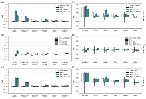
Figure 8 True, prior, and posterior annual budgets of fossil (a–b), biosphere (c–d), and total CO₂ (e–f) for the study domain, the sub-regions (b, d, f), and some of the largest European countries by area (a, c, e). The white bars show the true annual budgets based on the EDGAR and LPJ-GUESS flux products. The black bars represent the prior value of 0 PgC. The blue and green bars show the posterior budgets of ZBASE and ZCO2Only, respectively. The error bars represent the prior and posterior uncertainty calculated with a Monte Carlo ensemble of 100 members.

4.3 A realistic setup

The most realistic approach we can take to perform OSSEs is to use a realistic set of prior fluxes that differ substantially from the true fluxes used to generate the synthetic observations. In this section, we perform a series of experiments using the prior F_ff, F_bio, and F_biodis fluxes described in Sect. 3.1 to evaluate the impact of prescribing different prior fossil CO₂ uncertainty values as well as the impact of the prior F_biodis flux product (RndBASU) in the optimization of F_ff.

4.3.1 Impact of the prior fossil CO₂ uncertainty

Figure 9 shows the weekly F_ff time series for the three experiments using different prior uncertainties (BASE0.1, BASE0.21, and BASE0.3). The EDGAR (${\mathit{F}}_{\mathrm{ff}}^{\mathrm{t}}$) and ODIAC (prior) products have different temporal distributions along the year, with ODIAC being flatter than EDGAR, but both with a minimum during summer: for EDGAR in July (3.13 TgC d⁻¹) and for ODIAC in August (3.05 TgC d⁻¹). In the study domain (Fig. 9a), the posterior F_ff values for the three experiments are very close to each other and approach the truth from January to February and later from August to December. From May to August, there is an increment in the posterior fluxes that depart from ${\mathit{F}}_{\mathrm{ff}}^{\mathrm{t}}$, with the maximum difference in July that we find in western/central Europe (ranging from 0.10 for BASE0.1 to 0.17 TgC d⁻¹ for BASE0.3) and in eastern Europe (0.08 to 0.26 TgC d⁻¹) (Fig. 9). The posterior time series from the three experiments have the same RMSE with respect to the truth, 0.48 TgC d⁻¹, which is lower than the prior RMSE of 0.65 TgC d⁻¹. The posterior F_ff time series in western/central Europe shows the best results, with the estimates being close to the truth, except for June and July. The three experiments show the same performance, reducing the RMSE by 50 % (RMSE_prior = 0.26 TgC d⁻¹, RMSE_BASE0.1 = 0.13 TgC d⁻¹), but BASE0.21 and BASE0.3 show values farther from the truth in June and July. Northern Europe (Fig. 9c), on the other hand, shows priors that are already very close to the truth, with a posterior RMSE equal to the truth of 0.07 TgC d⁻¹. Finally, in eastern Europe, with the lowest sampling coverage, the three posterior time series degrade the prior estimate.

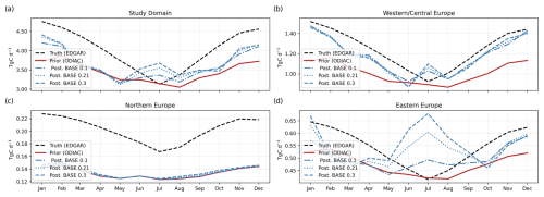
Figure 9 Monthly fossil CO₂ truth (dashed black lines), prior (solid red lines), and posterior fluxes from the BASE0.1 (dashed–dotted blue lines), BASE0.21 (dotted blue lines), and BASE0.3 (dashed blue lines) experiments for (a) the study domain and the three sub-regions: (b) western/central Europe, (c) northern Europe, and (d) eastern Europe (note the different scales on the y axis).

The difference in the annual budget of EDGAR and ODIAC for the study domain is 0.21 PgC for the year 2018, which is as large as the emissions of the country with the largest emissions in the study domain for the same year, Germany, with 0.23 PgC according to EDGAR and 0.19 PgC according to ODIAC (Fig. 10). This difference in the study domain is nearly recovered by all three experiments, with a recovery ranging from 30 % for BASE0.1 to 45 % for BASE0.3. In western/central Europe, the three experiments recover 96 % of the truth (around 71 % of the difference between true and prior), similar to Germany, where the recovery ranges from 94 % for BASE0.1 to 97 % for BASE0.3 (68 % to 82 % of the difference). As we find in the time series (Fig. 9d), the prior annual budget is very close to the truth in eastern Europe, where the difference is 0.02 PgC, and in Poland at 0.01 PgC. In both cases, the posterior recovers the annual budget, with overestimations from BASE0.3 for the whole sub-region and from BASE0.21 and BASE0.3 in Poland, which are as big as 120 %. Finally, and as expected from Fig. 9c and the prior uncertainty for the sub-region, there is no recovery of the annual budget in northern Europe further than the prior estimate.

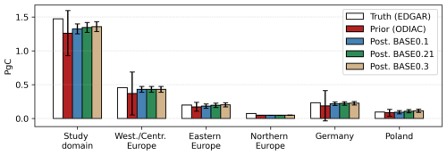
Figure 10 Total annual fossil CO₂ emissions for the study domain, western/central Europe, eastern Europe, northern Europe, Germany, and Poland. The white bars show the true emissions based on the EDGAR emission database. The red bars show the prior fluxes based on the ODIAC emission data product. The blue, green, and tan bars show the posterior fossil CO₂ emissions for the BASE0.1, BASE0.21, and BASE0.3 experiments, respectively. The error bars represent the prior and posterior uncertainty calculated with a Monte Carlo ensemble of 100 members.

4.3.2 Impact of the terrestrial isotopic disequilibrium product

The prior F_bio and F_biodis are very different in magnitude from the true values, with differences as large as 13.4 and 7.6 TgC d⁻¹, respectively, during summer for the whole study domain (Fig. 11d and g). This gap is well-resolved for F_bio in the study domain and western/central Europe (Fig. 11d and f) and has some underestimation in eastern Europe between June and September (Fig. 11e). However, for the posterior F_biodis we find some larger differences from the truth during June and September in the study domain and the two sub-regions. When we prescribe F_biodis (BASENoBD), the posterior F_ff values from June to August in the study domain and western/central Europe (Fig. 11a and b) get closer to ${\mathit{F}}_{\mathrm{ff}}^{\mathrm{t}}$ and after the summer in the study domain. This can also be seen in an improvement in the RMSE values, with 0.32 TgC d⁻¹ for the study domain and 0.10 TgC d⁻¹ for western/central Europe. In eastern Europe, the posterior F_ff for BASENoBD experiments does not show a significant improvement and, on the contrary, further degrades the prior estimate during the summer and the autumn.

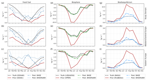
Figure 11 Monthly time series of F_ff (a–c), F_bio (d–f), and F_biodis (g–i) for the study domain (a, d, g), western/central Europe (b, e, h), and eastern Europe (c, f, i). The truth is represented by dashed black lines, the prior by solid red lines, posterior fluxes from BASE0.1 by dashed–dotted blue lines, and BASENoBD by dotted blue lines.

4.3.3 The observational space

Finally, we analyze the model's performance in the observational space at all sampling stations aggregated together, one polluted station (Saclay, SAC) (Fig. 12), and one background station (Jungfraujoch, JFJ) (Figs. 12 and 13) for the BASE experiment. We calculate two performance metrics: the correlation coefficient (R) between the synthetic observations and the prior and posterior simulated mixing ratios for all the sites and individually for the two sites selected and the reduced chi-square ${\mathit{\chi }}_{\mathit{\nu }}^{\mathrm{2}}$ for the overall simulation as a measure of the improvement upon the initial state and to guarantee that we are not under- or over-fitting the model (Table 5). We calculate the reduced chi-square as

$$\begin{array}{}\text{(10)}& {\mathit{\chi }}_{\mathit{\nu }}^{\mathrm{2}}={\displaystyle \frac{\mathrm{1}}{\mathit{\nu }}}\sum _{i=\mathrm{1}}^N{\left({\displaystyle \frac{{\mathit{y}}_i^{\mathrm{so}}-{\mathit{y}}_i^{\mathrm{b},\mathrm{a}}}{{\mathit{ϵ}}_i}}\right)}^{\mathrm{2}},\end{array}$$

where ${\mathit{y}}_i^{\mathrm{so}}$ is the synthetic observation i, ${\mathit{y}}_i^{\mathrm{b},\mathrm{a}}$ is either the prior (b) or the posterior (a) mixing ratio i, ϵ_i is the error of the synthetic observation i, N is the number of observations, and ν represents the degrees of freedom calculated as $\mathit{\nu }=N-p$, with p being the number of fitted parameters in the model. Since p is difficult to calculate due to the different time and space clusters, we keep the number of observations as the degrees of freedom (ν=N).

Table 5 Performance metrics (correlation coefficient R, standard deviation, and reduced chi-square ${\mathit{\chi }}_{\mathit{\nu }}^{\mathrm{2}}$) for all sites, Saclay (SAC), and Jungfraujoch (JFJ).

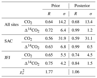
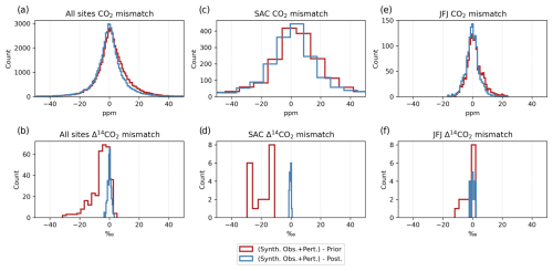
Figure 12 Mismatches between the synthetic observations and the prior (red) and posterior (blue) mixing ratios for all the sampling stations, Saclay (SAC) and Jungfraujoch (JFJ) for CO₂ (a, c, e) and for Δ¹⁴CO₂ (b, d, f). All prior and posterior mixing ratios correspond to the BASE experiment.

The histograms in Fig. 12 show the mismatches between the synthetic observations and the prior and posterior mixing ratios. For the CO₂ mixing ratios at all sites (Fig. 12a), the histogram shows a distribution centered around zero for both prior and posterior mismatches, with a standard deviation of 14.2 and 13.4, respectively (see Table 5), indicating systematic deviations from the observed values. The posterior mismatch has a slightly tighter distribution, suggesting a small improvement in the model after adjustments, as reflected in the correlation coefficient (Table 5). At Saclay (Fig. 12c), the mismatch distribution is wider than the aggregate of all sites, which could suggest greater variability or larger errors at this particular site. The posterior adjustment has not significantly tightened the distribution, indicating that the model adjustments did not perform as well at this site as they did on average across all sites. On the other hand, the distribution in Jungfraujoch (Fig. 12e) is much tighter than at all sites and SAC, with the posterior mismatch displaying a slight improvement in precision as evidenced by the narrower spread. However, when comparing the posterior time series with the synthetic observations before adding the random perturbation (Fig. 13a and c), there is better agreement between them than with the prior values, especially during periods of higher variability (April to July at SAC and April to September at JFJ).

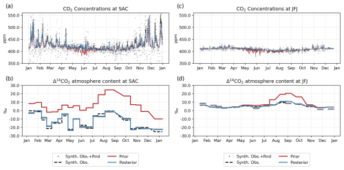
Figure 13 Mixing ratio time series of CO₂ (a, c) and Δ¹⁴CO₂ (b, d) at Saclay (SAC) and Jungfraujoch (JFJ), respectively. All prior and posterior mixing ratios correspond to the BASE experiment.

The Δ¹⁴CO₂ synthetic observations are in general better fitted by the posterior than CO₂ at all sites, SAC, and JFJ (Table 5). In all cases, the prior distribution is displaced to negative values, indicating that the prior simulated values are in general higher than the synthetic observations as shown for the whole period at SAC (Fig. 12d) and from July to November at JFJ (Fig. 12f). These larger prior mixing ratios are mainly caused by the prior terrestrial disequilibrium flux from July to November and by the nuclear production flux throughout the year, which is significantly larger at Saclay (Fig. 14). However, the posterior mismatches showed a much narrower spread around zero at all sites (Fig. 12b), Saclay (Fig. 12d), and Jungfraujoch (Fig. 12f) that is evident in the time series at both sites where the posterior closely follows the synthetic observations, as supported by the correlation coefficients (Table 5).

The reported ${\mathit{\chi }}_{\mathit{\nu }}^{\mathrm{2}}$ values of 1.77 for the prior and 1.06 for the posterior across all sites and samples suggest a substantial improvement in the model's performance in adjusting the prior mixing ratios to the synthetic observations. A ${\mathit{\chi }}_{\mathit{\nu }}^{\mathrm{2}}$ of 1.77 for the prior indicates that there were significant discrepancies between the prior and the synthetic observations. This is consistent with the broader spread of mismatches in the histograms for both SAC and JFJ sites, as well as the apparent overestimation of Δ¹⁴CO₂ content in the time series. The improvement to a ${\mathit{\chi }}_{\mathit{\nu }}^{\mathrm{2}}$ of 1.06 for the posterior indicates a better fit to the synthetic observations that is likely to be reflective of the underlying data patterns while still maintaining some degree of generalizability without over-fitting the data.

Figure 14 Contribution of each category to the prior Δ¹⁴CO₂ simulated mixing ratios at Saclay (a) and Jungfraujoch (b).

5 Discussion

Under the current sampling strategy and observation network, we demonstrate through OSSEs that adding Δ¹⁴CO₂ observations can help us constrain fossil CO₂ emissions over Europe using the LUMIA system. We start with two simulation experiments in which we set the prior fossil CO₂ and biosphere (net ecosystem exchange, NEE) fluxes to zero: ZBASE and ZCO2Only. Under an OSSE setup, even when using completely different truth and prior flux products (e.g., different spatiotemporal distributions and annual budgets), due to assumptions such as a perfect transport model and background mixing ratios, it is easy for the model to retrieve the true values even without adding Δ¹⁴CO₂ observations. For this reason, we set up these two more challenging experiments to assess the capabilities of the inversion system to constrain the fossil CO₂ emissions and biosphere fluxes using CO₂ and Δ¹⁴CO₂. The ZBASE and ZCO2Only experiments show us that in regions with a dense sampling network, such as western/central Europe, when adding Δ¹⁴CO₂ observations, LUMIA is capable of recovering the seasonality of F_ff and F_bio, as well as the total annual CO₂ budget of the whole region and some of the larger countries (also in terms of fossil CO₂ emissions) such as Germany and France. On the other hand, the results in northern Europe, which has relatively good network coverage, are not as good as in western/central Europe regarding fossil CO₂. Comparing the ranges of the true fossil CO₂ and biosphere fluxes in northern and western/central Europe, we find that, while ${\mathit{F}}_{\mathrm{bio}}^{\mathrm{t}}$ has a similar range in both regions, ${\mathit{F}}_{\mathrm{ff}}^{\mathrm{t}}$ differs by 1 order of magnitude. Using the concept of the signal-to-noise ratio, if we consider the fossil CO₂ to be the signal (the variable in which we are more interested) and the biosphere to be the noise, this difference of 1 order of magnitude between them in northern Europe makes it easier for the model to recover the biosphere fluxes than the fossil CO₂ emissions, even with additional information about Δ¹⁴CO₂. In addition, the prior uncertainty, which is proportional to the fluxes, is close to zero for the fossil fluxes, while it is 2 orders of magnitude larger for the biosphere, making it more costly for the inversion to constrain the fossil CO₂ emissions.

The inversions are able to resolve the NEE at the continental level and in the sub-regions but struggle more with fossil emissions in some regions with few observations (e.g., southern Europe and the British Isles). This is similar to what was found by Wang et al. (2018) despite the differences between their inversion implementation and our LUMIA system. The main differences lie in the transport model and the inversion approach. They use a global transport model at a resolution of 3.75° × 2.5° (Laboratoire de Météorologie Dynamique’s LMDZv4) and a pre-calculated fossil CO₂ tracer (product of the mass balance), while we use a Lagrangian regional transport model at a higher horizontal resolution (0.5° × 0.5°) and optimize both the fossil and the natural fluxes using CO₂ and Δ¹⁴CO₂ as tracers. Wang et al. (2018) found the largest error reductions around Germany, Benelux, and eastern France, where most sampling stations are located. Northern Europe was also poorly constrained in their inversions, similar to what we find. Wang et al. (2018) attributed the results in northern Europe to the coarse spatial resolution of the transport model. But even with a higher-resolution transport model as employed in LUMIA, we still cannot resolve the true fossil CO₂ emissions in an OSSE setup given the current CO₂ and Δ¹⁴CO₂ observation networks. We think that a more likely explanation is the difference in the magnitude of the fossil CO₂ emissions in this region against the natural fluxes. This can be seen by the differences in the seasonal amplitude of the fluxes. In western/central Europe F_bio and F_ff are of a similar order of magnitude (2.81 TgC d⁻¹ for F_bio and 0.6 TgC d⁻¹ for F_ff) (see Figs. 5 and 6). In contrast, in northern Europe, there is a 10-fold difference in the seasonal amplitude of the two fluxes: 2.44 TgC d⁻¹ for F_bio and 0.06 TgC d⁻¹ for F_ff. In addition, the prior uncertainty for F_ff (0.002 PgC yr⁻¹) in this region is much lower compared to F_bio (0.12 PgC yr⁻¹) in northern Europe.

The BASE experiments, in which we use realistic prior fluxes, show that the posterior fossil CO₂ emissions are not very sensitive to the prescribed prior uncertainty in regions with a dense sampling network, even when using a low prior F_ff uncertainty in which case it is more difficult for the inversion algorithm to recover the true fluxes. As we have observed in previous studies using LUMIA (Monteil et al., 2020; Monteil and Scholze, 2021), the cost of fitting the observations dominates the total cost function value. In this sense, the relative value of the prior uncertainty of F_bio against F_ff is going to significantly impact the spatiotemporal distribution of flux adjustments, but the total uncertainty of the fluxes is of lesser importance since the model has enough freedom to adjust the data. In other words, the error structure and how it is set up for the different flux categories is going to have more of an impact than the total prior uncertainty. Both Basu et al. (2016) and Wang et al. (2018) highlight the importance of a regional horizontal correlation and error structure for fossil CO₂ emissions. In our study, we use the same horizontal correlation and error structures originally developed by Monteil et al. (2020) for NEE. We are aware of the necessity of defining specific structures for fossil CO₂ within LUMIA due to the low improvement in spatial terms that we find in Fig. 7 when adding Δ¹⁴CO₂ observations. However, it is important to mention that given the sparse observation network, we can expect spatial misattributions (flux corrections that should happen in one place but are instead made elsewhere), and therefore we should interpret the results aggregated at the scale that is relevant given the model setup, as we demonstrate through the time series and annual budget results. Such spatial misattribution is illustrated in the spatial RMSE reduction results for the biosphere fluxes. We can clearly identify the formation of dipoles (clusters of larger RMSE values) in regions with no observations such as the southern part of the study domain and the Baltic States, indicating that these areas are underconstrained.

We also find the prior terrestrial disequilibrium product to have an important impact on the posterior fossil CO₂ emissions (Fig. 11). The prior terrestrial isotopic disequilibrium flux in our experiments is intentionally incorrect with the aim of showing the impact that it can have in the estimation of fossil CO₂ emissions. As shown in Fig. 11, the maximum difference between the prior and the true F_biodis is of the same order of magnitude for western/central Europe (2.1 TgC d⁻¹) and eastern Europe (1.3  TgC d⁻¹) in July. For F_ff, however, the difference between the prior and truth is about 1 order of magnitude larger for western/central Europe compared to eastern Europe (0.03 TgC d⁻¹ vs. 0.005 TgC d⁻¹). This larger difference causes a stronger dilution of the fossil emissions in eastern Europe and therefore essentially lowers the signal-to-noise ratio of the Δ¹⁴CO₂ measurements; added to the lower network coverage compared to western/central Europe, it leads to a poorer constraint of the fossil CO₂ emissions. As also seen in Fig. 9, this is particularly evident in eastern Europe during the summer months, where the fossil CO₂ signal is further convoluted by the large biospheric uptake, making it more difficult to accurately constrain fossil emissions in this region. According to Turnbull et al. (2009), one of the main contributors to atmospheric Δ¹⁴CO₂ is heterotrophic respiration in natural environments. Therefore, having a good prior F_biodis estimate is crucial in estimating posterior F_ff. The impact of F_biodis and the other Δ¹⁴CO₂ flux terms is not negligible; in particular, the emissions from nuclear facilities can have a larger impact than the terrestrial disequilibrium (Graven and Gruber, 2011), as was evident when analyzing the individual impacts of the flux categories, showing that at sampling sites heavily influenced by emissions from nuclear facilities such as Saclay, these emissions can be as large as the terrestrial isotopic disequilibrium fluxes. In this study, we fixed the F_nuc term (i.e., we use the same fluxes for calculating the synthetic observations and in the inversions), and hence its impact is not considered here. In previous studies (Wang et al., 2018; Basu et al., 2016, 2020) the F_nuc is usually prescribed and assumed to be an annual value at each nuclear facility location (Graven and Gruber, 2011; Zazzeri et al., 2018) due to a lack of knowledge on the temporal distribution of these emissions. This variability in nuclear emissions has only been studied by measuring the atmospheric content of Δ¹⁴CO₂ in the surrounding areas of single nuclear facilities (Turnbull et al., 2014; Vogel et al., 2013; Lehmuskoski et al., 2021), but not yet in a large regional setup, and therefore it needs further investigation.

The observing system simulation experiment (OSSE) framework used in this study assumes a perfect realization of atmospheric transport and mixing processes by employing the same transport model across the simulations. This assumption simplifies the complex nature of atmospheric dynamics and is a common approach to limit the scope of variability in such studies. However, it is crucial to acknowledge that this simplification overlooks one of the largest sources of uncertainty in atmospheric inverse modeling: the accurate representation of atmospheric transport and mixing processes. The variability and uncertainty in atmospheric transport can significantly impact the estimation of greenhouse gas sources and sinks. As demonstrated by Schuh et al. (2019), inconsistencies in transport simulations can introduce systematic biases in surface flux estimations, which can be as substantial as 1.7 PgC yr⁻¹ for large zonal bands. In a study by Munassar et al. (2023), in which multiple combinations of global and regional models were tested using two different inversion frameworks (LUMIA and CarboScope-Regional – CSR), they found that using a different regional transport (FLEXPART and STILT – Stochastic Time-Inverted Lagrangian Transport) model can cause differences in the posterior NEE annual budget of 0.51 PgC yr⁻¹. This highlights the sensitivity of inversion-derived emission estimates to the accuracy of the transport model used and emphasizes the critical role that transport uncertainty plays across global flux inversion systems.

Furthermore, the assumption of perfect boundary conditions in the model presents another significant simplification. Boundary conditions in atmospheric modeling can greatly influence the mixing ratio gradients and flux estimates, and their mischaracterization can propagate errors throughout the model domain. Coming back to the study by Munassar et al. (2023), the use of a different global transport model (TM3 and TM5) for the estimation of the boundary condition can cause discrepancies in the posterior annual budget as large as 0.23 PgC yr⁻¹. Errors in these aspects of the transport model could lead to skewed emission estimates. Given these considerations, the presented results should be interpreted with caution, understanding that the true uncertainty in atmospheric inverse modeling is likely understated in these OSSEs. It underscores the need for more comprehensive approaches that account for transport model uncertainties, such as employing ensemble modeling techniques that incorporate multiple transport models and boundary conditions to better capture the inherent uncertainties in atmospheric dynamics (Locatelli et al., 2015; Aleksankina et al., 2018).

6 Conclusions and future perspectives

We have expanded the LUMIA system to be capable of simultaneously inverting atmospheric observations of CO₂ and Δ¹⁴CO₂ to estimate fossil CO₂ emissions and net terrestrial biosphere CO₂ fluxes over Europe. We performed the first observing system simulation experiments to test the performance of the Δ¹⁴C-enhanced LUMIA version. In the first set of experiments, we show the impact of adding Δ¹⁴C observations in a scenario with prior estimates of F_ff and F_bio set to zero. In regions with good sampling network coverage, assimilating both CO₂ and Δ¹⁴C observations allows recovering the seasonality of F_ff and F_bio and the annual F_ff budget, while when assimilating only CO₂ observations, the posterior F_ff is degraded. In the second set of experiments, we performed OSSEs using more realistic priors to test the impact of the prescribed F_ff uncertainty and the impact of the prior F_biodis product. The prescribed prior uncertainty has no significant impact on the posterior F_ff. On the other hand, the prior F_biodis product can significantly impact the posterior F_ff.

The purpose of this study is to describe the multi-tracer, more specifically CO₂ and Δ¹⁴CO₂, version of LUMIA and illustrate its application to estimate both fossil CO₂ emissions natural CO₂ fluxes simultaneously. Future work should analyze in more detail the impact of various aspects of our inversion setup here, such as the assumption of a perfect transport model, the specification of the boundary conditions, and different spatiotemporal error structures, on the posterior fossil CO₂ emissions and natural CO₂ fluxes. Particular emphasis should be placed on the analysis of the impact of the prior F_biodis product using simulated terrestrial biosphere disequilibrium estimates by, e.g., the LPJ model following the methodology by Scholze et al. (2003) because our study here illustrated the importance of this flux term in the CO₂ and Δ¹⁴CO₂ inversion. In addition, the impact of the prior F_nuc, the sampling strategy, and the network density of the Δ¹⁴C observations on the capability to estimate fossil CO₂ emissions needs to be evaluated. The current 2-weekly integrated sampling strategy allows us to get a reasonable estimate of the annual budget over the whole domain. But the inversion can recover neither the correct temporal behavior nor the spatial distribution of the fossil CO₂ emissions when using CΔ¹⁴C observations provided by the current 2-weekly integrated sampling strategy. Additionally, converting Δ¹⁴CO₂ values to CΔ¹⁴C implies calculating the average of the CO₂ observations during the 2-week integration period, which can introduce additional errors that we did not account for in this study. We will evaluate the use of hourly flask samples under different strategies as described by Levin et al. (2020), such as a “smart” sampling based on pollution episodes of CO₂ and CO. This will be in preparation for the intensive Δ¹⁴CO₂ sampling campaign (hourly samples taken every third day) planned within the EC's Horizon Europe CORSO (CO2MVS Research on Supplementary Observations) project (https://corso-project.eu/, last access: 7 January 2025) during 2024 at 10 ICOS stations located in western Europe.

Appendix A: Summary of ocean and ocean-disequilibrium-derived synthetic observations

Table A1 Summary of ocean and ocean-disequilibrium-derived synthetic observations across sampling stations used in this study. The table compares average ocean CO₂ and Δ¹⁴C values, ocean disequilibrium (Ocedis) Δ¹⁴C values, and synthetic total CO₂ and Δ¹⁴C observations, along with their random noise variants and associated observation errors. Values are presented as averages across all stations and for individual sampling stations, including their standard deviations. These data provide insight into the variability of ocean and ocean disequilibrium contributions relative to total synthetic observations.

Appendix B: Spatial clustering algorithm

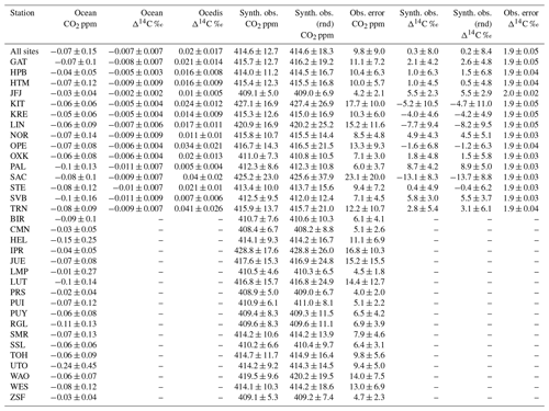
The inversion solves for offsets to the prior fluxes at a variable spatial resolution: high (up to 0.25°) in the direct vicinity of observation sites but lower in parts of the domain that are not well-sampled by the observation network. To achieve this, the spatial domain of the inversion is divided into a set of clusters of grid cells, each defined by the following properties.

• Cells: the list of grid cells included in the cluster.

• Weight: the sum of a property carried by each grid cell. In our case, this property is the average sensitivity of the observation network to that grid cell.

• Size: the number of grid cells in the cluster.

• mean_lat and mean_lon: the average (area-weighted) latitude and longitude of the grid cells in the cluster.

• Area: the total of all the grid cells included in the cluster.

• Type: ocean, land, or mixed.

• Continuity: whether it is possible to “walk” from any grid cell of the cluster to any other one or whether there are discontinuities (e.g., a “land” cluster separated into two parts by ocean grid cells).

The objective of the clustering algorithm is to divide the domain into a user-defined number of continuous clusters with roughly equal “weight”. The weight of a single grid cell is, in our case, defined as the average value of the adjoint field in that grid cell for an adjoint simulation driven by model–data mismatches set proportional to the uncertainty of each observation. The clustering is performed iteratively as follows.

1. Initially, one single cluster is formed, comprising all grid cells of the domain. It is added to a pool of “dividable” clusters.

2. The weight of all clusters in that pool is calculated (i.e., the weight of the single initial cluster at the first iteration).

3. The cluster with the largest weight is then split into two even parts across its longest axis (i.e., in an eastern and western part, at the first iteration).

4. The resulting two new clusters are checked for continuity. If needed, they are further split into several continuous clusters.

5. If a cluster reaches the minimum size (1 grid cell), it is moved to a pool of “defined” clusters.

6. If the total number of clusters (dividable plus defined) is lower than the target number of clusters, then repeat steps 2 to 6. Otherwise, exit.

Because of how the cluster weights are defined, clusters away from observation points end up being considerably larger, but they are in regions where the inversions would have applied very smooth flux adjustments, so there is no real drawback to this clustering.