Stratospheric circulation response to large Northern Hemisphere high-latitude volcanic eruptions in a global climate model

Stratospheric aerosols after major explosive volcanic eruptions can trigger climate anomalies for up to several years following such events. Whereas the mechanisms responsible for the prolonged response to volcanic surface cooling have been extensively investigated for tropical eruptions, less is known about the dynamical response to high-latitude eruptions. Here we use global climate model simulations of an idealized 6-month-long Northern Hemisphere high-latitude eruption to investigate the stratospheric circulation response during the first three post-eruption winters. Two model configurations are used, coupled with an interactive ocean and with prescribed sea-surface temperature. Our results reveal significant differences in the response of the polar stratosphere with an interactive ocean: the surface cooling is enhanced and zonal flow anomalies are stronger in the troposphere, which impacts atmospheric waveguides and upward propagation of large-scale planetary waves. We identify two competing mechanisms contributing to the post-eruption evolution of the polar vortex: (1) a local stratospheric top-down mechanism whereby increased absorption of aerosol-induced thermal radiation yields a polar vortex strengthening via thermal wind response and (2) a bottom-up mechanism whereby anomalous surface cooling yields a wave-activity flux increase that propagates into the winter stratosphere. We detect an unusually high frequency of sudden stratospheric warmings in the simulations with interactive ocean temperatures that calls for further exploration. In the coupled runs, the top-down mechanism dominates over the bottom-up mechanism in winter 1, while the bottom-up mechanism dominates in the follow-up winters.

1 Introduction

The enhancement of the stratospheric aerosol layer following strong sulfur-rich explosive volcanic eruptions is an important driver of natural climate variability due to the short-lived yet possibly very strong radiative anomalies imposed within the atmospheric column (Robock, 2000; Timmreck, 2012; Zanchettin, 2017). This direct radiative effect can alter both meridional surface and stratospheric temperature gradients that can, in turn, initiate further dynamical climate responses on seasonal to decadal timescales (Church et al., 2005; Gleckler et al., 2006; Stenchikov et al., 2009; Shindell et al., 2004; Otterå et al., 2010; Zanchettin et al., 2012; Swingedouw et al., 2015). Direct radiative and dynamical responses critically depend on the spatiotemporal characteristics of the enhanced stratospheric aerosol layer, which ultimately depends on the characteristics of the eruption, such as magnitude, timing, and location (Stenchikov et al., 2009; Shindell et al., 2004; Zanchettin et al., 2012; Swingedouw et al., 2015). Spatiotemporal characteristics of volcanic aerosol from high-latitude (HL), Northern Hemisphere (NH) eruptions are typically very different when compared to tropical eruptions. Accordingly, several studies have shown that HL eruptions typically initiate different climate responses compared to tropical eruptions (Meronen et al., 2012; Pausata et al., 2015; Guðlaugsdóttir et al., 2018; Zambri et al., 2019; Sjolte et al., 2021). Therefore, tropical eruptions cannot be considered close analogs of HL eruptions, underlining the need for more studies on the latter to further quantify their potential climate impacts (Zanchettin et al., 2016). In this study we explore how stratospheric sulfate aerosol enhancements largely constrained in the NH extratropics affect hemispheric-scale atmospheric dynamics, with a focus on the stratospheric polar vortex and on temporal evolution of responses through three perturbed winters.

The winter stratospheric polar vortex is considered to play a deciding role in distinguishing between the response to low- and high-latitude NH enhancements of the stratospheric sulfate aerosol layer, where opposite responses are expected to emerge under the same mechanism: when the stratospheric sulfate aerosol layer is enhanced at low latitudes, e.g., following tropical volcanic eruptions, local warming by infrared absorption increases the meridional stratospheric temperature gradient that can lead to a stratospheric polar vortex strengthening due to a thermal wind response (e.g., Zanchettin et al., 2012; Bittner et al., 2016a). Conversely, the local warming from aerosols constrained at higher latitudes decreases the meridional temperature gradient, promoting a weakening of the polar vortex (Kodera, 1994; Perlwitz and Graf, 1995; Stenchikov et al., 2002; Oman et al., 2005; Sjolte et al., 2021). The downward propagation of the stratospheric polar vortex anomaly into the troposphere can lead to regime shifts of the tropospheric Arctic Oscillation and associated anomalous regional surface patterns (e.g., Zanchettin et al., 2012; Zambri et al., 2017). In the case of polar vortex weakening, a critical role is attributed to the increased likelihood of sudden stratospheric warming events (SSWs) (Haynes, 2005; Domeisen et al., 2020; Huang et al., 2021; Kolstad et al., 2022, and references therein), whose projection on a negative Arctic Oscillation is expected to bring a series of consequences, including increased frequency of tropospheric blockings and mid-latitude cold-air outbreaks (e.g., Ma et al., 2024). However, the negative Arctic Oscillation and associated tropospheric anomalies following SSWs are characterized by a low signal-to-noise ratio (e.g., Charlton-Perez et al., 2018; Zhang et al., 2019). Accordingly, recent studies tend to disagree on this top-down mechanism being a robust dominant feature of climate response to volcanic eruptions (Weierbach et al., 2023; DallaSanta and Polvani, 2022; Kolstad et al., 2022; Azoulay et al., 2021; Polvani et al., 2019; Zanchettin et al., 2022; Toohey et al., 2014). The radiative surface cooling following large volcanic eruptions has been shown to affect the stratospheric polar vortex via a bottom-up mechanism (e.g., Graf et al., 2014; Peings and Magnusdottir, 2014; Omrani et al., 2022). An example of this bottom-up mechanism following HL eruptions is demonstrated in Sjolte et al. (2021), where they linked a weak polar vortex to an increase in wave energy flux from the troposphere into the stratosphere without the meridional stratospheric temperature gradient playing a major role.

With this in mind, the importance of transient atmospheric eddies (waves) and eddy–mean-flow interactions is becoming increasingly clear in explaining vertical and horizontal propagation of atmospheric perturbations of various origins (e.g., Smith et al., 2022; Nakamura, 2024). DallaSanta et al. (2019) used a hierarchy of simplified atmospheric models to show that eddy feedbacks are crucial in explaining stratosphere–troposphere coupling as well as the stratospheric response alone following a tropical Pinatubo-like eruption. This demonstrates that the anomalous atmospheric circulation response to an enhanced stratospheric sulfate aerosol layer cannot be understood as the mere adjustment to meridional temperature gradients and that eddy–mean-flow interactions and eddy feedback are an essential contribution to such response. Both mechanisms, i.e., the top-down mechanism triggered by local stratospheric heating and the bottom-up mechanism triggered by surface cooling, act together in the real world and in realistic simulations. Therefore, idealized model experiments are required to assess their relative contribution to uncertainty in regional climate variability during the period following the enhancement of the sulfate aerosol layer (Zanchettin et al., 2016).

Icelandic volcanism has played a role in shaping past NH climate variability and will continue doing so. Two Icelandic eruptions during the past 2000 years, namely Eldgjá in ∼ 939 CE and Laki in 1783 CE, are considered to have had a significant impact on climate variability up to the global scale (Brugnatelli and Tibaldi, 2020; Zambri et al., 2019; Oppenheimer et al., 2018; Thordarson and Self, 2003; Stothers, 1998). These types of effusive eruptions are common in Iceland, where their duration can extend over years. During part of the eruption time, such eruptions can become explosive (referred to as mixed-phase eruptions) when ascending magma in a conduit comes in contact with water, as was considered the case with both Eldgjá and Laki, explaining their widespread impacts. The eruption history and dense monitoring network of Icelandic volcanic systems tell us that many of these systems are currently on the verge of an eruption, having already produced some of the largest volcanic eruptions over the past millennia (e.g., Öræfajökull, Bárðarbunga, and Hekla; Larsen and Gudmundsson, 2014; Barsotti et al., 2018; Einarsson, 2019).

Therefore, history and current activity makes these types of eruptions an ideal reference case to explore the potential climatic impacts of HL enhancements of the stratospheric sulfate aerosol layer and to test hypotheses about the underlying mechanisms driving the climate response. This is the focal point of this study, where we investigate for the first time the role of wave–mean-flow interactions and SSWs in the climate response to a HL volcanic eruption. For this we perform idealized, long-lasting, HL volcanic perturbation experiments using the Community Earth System Model version 1 (CESM1) in its coupled and atmosphere-only configurations. We evaluate the NH response during the first three winters following the eruption, referred to as post-eruption winters in the text, and assess the dominating mechanism in each winter. This paper is organized as follows: Sect. 2 describes the model, experimental design, and diagnostics; results are presented in Sect. 3, followed by discussions in Sect. 4; and we end with concluding our results in Sect. 5.

2 Methods

2.1 Numerical model

We use the Community Earth System Model (CESM) version 1, developed by the National Center for Atmospheric Research (NCAR). In our configuration of CESM1, the atmospheric component is the Whole Atmosphere Community Climate Model version 4 (WACCM4, Marsh et al., 2013). WACCM4 includes 66 vertical levels (up to 5.1 × 10⁻⁶ hPa, ∼ 140 km) and uses CAM4 physics. We use the specified chemistry version of WACCM4 (SC-WACCM4), which is computationally less expensive to run but simulates dynamical stratosphere–troposphere coupling and stratospheric variability like SSWs and the polar vortex with skills comparable to the interactive chemistry model version (Smith et al., 2014). CESM1-WACCM4 uses the Community Atmospheric Model Radiative Transfer (CAMRT) to parameterize the radiative forcing where it has been shown to accurately represent stratospheric aerosols by, e.g., simulating the temperature response following Mt. Pinatubo in 1991 (Neely et al., 2016). The SC-WACCM4 experiments are run with a horizontal resolution of 1.9° latitude by 2.5° longitude and include present-day (year 2000) radiative forcing. A repeating 28-month full cycle of the Quasi-biennial Oscillation (QBO) is included in the SC-WACCM4 experiments through nudging of the equatorial stratospheric winds to observed radiosonde data. In the coupled ocean–atmosphere configuration, the ocean component of CESM1 is the Parallel Ocean Program version 2 (POP2). CESM1 also includes the Los Alamos sea-ice model (CICE), the Community Land Model version 4 (CLM4), and the River Transport Model (RTM). CLM is run at a horizontal resolution of 1.9° × 2.5°, and POP2 and CICE are run at a nominal 1° resolution, with a higher resolution near the Equator than at the poles. Further details about CESM1 are given in Hurrell et al. (2013).

2.2 Volcanic forcing file

We use the Easy Volcanic Aerosol (EVA) forcing generator (Toohey et al., 2016). EVA provides zonally symmetric stratospheric aerosol optical properties as a function of time, latitude, height, and wavelength (see detailed information on the tool in Toohey et al., 2016). EVA has been used to generate volcanic forcing in both idealized volcanic experiments (e.g., Zanchettin et al., 2016) and realistic paleoclimate simulations (Jungclaus et al., 2017), contributing to the sixth phase of the coupled model intercomparison project.

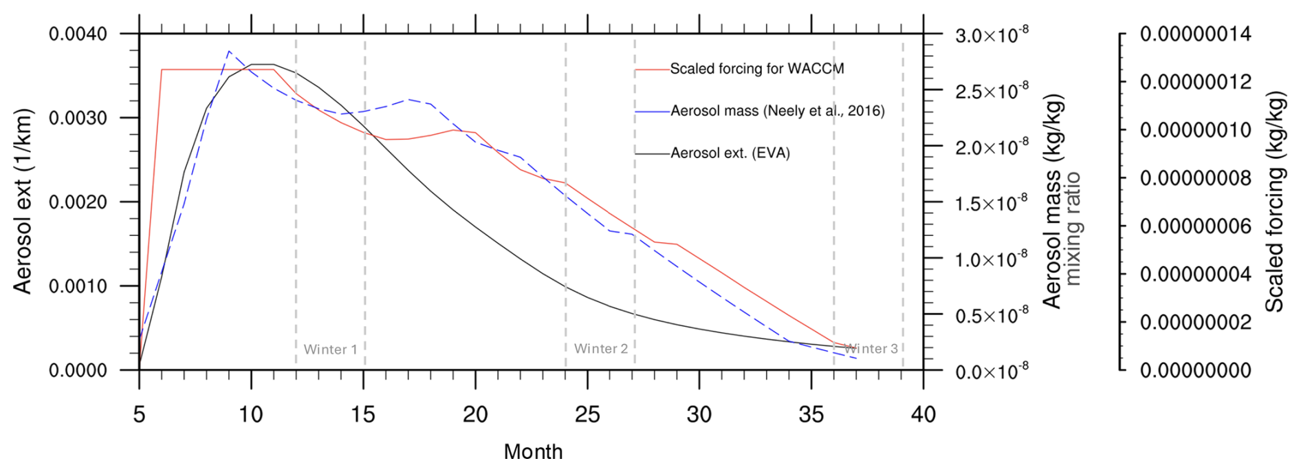
Figure 1 The time series of the original EVA aerosol extinction output (1 km⁻¹, black curve) and the dry aerosol mass mixing ratio of the volcanic forcing file of Neely et al. (2016) (kg kg⁻¹, dashed blue curve) used for deriving the linear scaling coefficient for the conversion of EVA output into WACCM4 input (kg kg⁻¹, red curve). The horizontal axis is time (months) from the start of the eruption. Here we assume that the aerosol lifetime at 65° N is the same as at 45° N. Dashed vertical lines show the three winters that we focus on in this study.

We use EVA to prescribe the volcanic aerosol loading corresponding to that of the 1991 Mt. Pinatubo eruption (14.04 Tg SO₂) but at 45° N. Since the model reads the volcanic forcing as the aerosol mass mixing ratio (kg kg⁻¹) while our EVA output is in 1 m⁻² (aerosol extinction), we scale our forcing file by using the standard aerosol input file for CAM4 and 5 (see Neely et al., 2016, Table 1) for the same eruption. A monthly scaling factor was derived from this linear relationship between the aerosol extinction and the aerosol mass mixing ratio that was used to scale the raw EVA forcing data (Fig. 1). From these scaled forcing data, the aerosol optical properties for our experiments are obtained with a two-step approach. First, we move the injection location northwards so that the center of the aerosol mass is at 65° N latitude and spans 10–28 km in altitude. Then, we define the start of the eruption to be 1 May and prolong the peak of the forcing by extending in time the highest monthly value in the so-obtained forcing data, so that the decline in aerosol mass begins 6 months after the start of the eruption or on 1 November (see Fig. 1). We thus obtain aerosol optical properties for an idealized, long-lasting, high-latitude NH eruption. In this experiment we assume stratospheric injection only, although similar eruptions in the natural world would likely inject part of the total aerosol mass within the troposphere during the eruption. Past NH eruptions like Eldgjá and Laki had an atmospheric SO₂ loading of 219 and 122 Tg, respectively, that was carried aloft with the eruptive column up into the upper troposphere, with portions of the aerosols reaching the lower stratosphere during the eruptions (Thordarson et al., 2001). Hence our experiment can also be considered a 6-month stratospheric aerosol injection that is analogous to similar although smaller eruptions (as compared to Laki) without the tropospheric aerosols.

2.3 Experimental design

We ran two volcanic perturbation experiments with CESM1. The first experiment is conducted with the atmosphere-only version of the model, where boundaries to SC-WACCM4 are provided by prescribed fields of sea-surface temperature (SST) and sea-ice concentration (SIC) corresponding to the 1979–2008 monthly climatology of HadISST observations (Rayner et al., 2003). We refer to this experiment as atm-only. The second experiment is conducted with the coupled version of the model, henceforth referred to as cpl. For each experiment we run 20 ensemble members including the volcanic forcing and 20 paired ensemble members without the volcanic forcing and otherwise identical to the volcanic simulations, which we refer to as the control.

The atmosphere-only experiments were run over 3 full years, which provides two full winters after the onset of the eruption. We found that there was no need to extend the simulations further given the duration of the forcing and short memory of the atmosphere. The coupled experiments follow a similar protocol, but they were integrated over 15 years to assess the response influenced by oceanic dynamical adjustment. However, in this study we only focus on the first three winters following the eruption, where the January and February forcing of winter 3 are defined to be a continuation of the December value of year 2. We define the first post-volcanic winter as December of the starting year (year 0) and the following January and February (year 1); the second post-volcanic winter is then December of year 1 and the following January and February of year 2.

Because the QBO is prescribed, and given its importance for the atmospheric circulation and the distribution of volcanic aerosols within the stratosphere (Thomas et al., 2009; DallaSanta et al., 2019; Brown et al., 2023), we have been careful in homogeneously sampling the QBO phasing that is imposed on the 20 ensemble members. For this, we shift the 28-month QBO cycle by 1 month for every ensemble member, so that the phasing of the QBO differs from one ensemble member to the next (Elsbury et al., 2021a). This avoids potential biases in the climatic response that may be induced by any dominating QBO phase.

2.4 Diagnostics

Model output is analyzed by computing paired anomalies, defined as deviations of each volcanic simulation from the corresponding control simulation (Zanchettin et al., 2022) (volcanic minus control). The statistical significance of the ensemble mean of paired anomalies is assessed at the 95 % confidence interval, calculated from all 20 ensemble members, using a two-sided Student t test in addition to a Kolmogorov–Smirnov test.

To evaluate the effects of planetary waves on the zonally averaged stratospheric response, we use the Eliassen–Palm (EP) flux and its divergence (Edmon et al., 1980), in addition to the 3D generalization of the EP flux, the Plumb flux (Plumb, 1985), for a longitudinal representation in the lower troposphere and stratosphere. We identify SSW events by using an algorithm following the procedures described in Charlton and Polvani (2007), where mid-winter sudden warming events are determined to take place if the 10 hPa zonal-mean zonal wind at 60° N becomes easterly. Once a warming is identified, no day within 20 d of a central date, defined as the first day in which the daily mean zonal-mean wind at 60° N and 10 hPa is easterly, can be defined as an SSW. Changes in conditions for large-scale planetary wave propagation (waveguides) are examined using the optimal propagation diagnostic for stationary planetary waves, described in Karami et al. (2016). This metric is based on the construction of probability density functions for positive values of the refractive index (Matsuno, 1970), as a function of zonal and meridional wave numbers. The refractive index is calculated using daily zonal wind and temperature at all levels to derive monthly and zonally averaged probabilities for stationary Rossby waves to propagate through the atmosphere, as a function of latitude and pressure level. This is calculated for zonal wave numbers k = 1, 2, and 3 and meridional wave numbers l = 1, 2, and 3 (large-scale waves), and we average the probabilistic refractive index for each of the nine combinations of k and l to provide a general estimate of chances for propagation of stationary planetary waves. For the eddy feedback calculations we compute the square of the local correlation across the ensemble members between DJF zonal-mean zonal wind and the divergence of the northward EP flux (δϕFϕ) averaged over 600–200 hPa (Smith et al., 2022). In addition, we compute the rate of temperature (K) changes in the 2 m temperature (T_2 m​​​​​​​) gradient using spherical harmonics to yield a T_2 m gradient in the meridional ($\mathrm{d}Z/\mathrm{dlat}$) and zonal ($\mathrm{d}Z/\mathrm{dlon}$) directions.

3 Results

In the following sections we will investigate the cpl experiment to characterize the forced response and identify the mechanism by utilizing the information provided by the atm-only experiment. We begin our investigation in the upper atmosphere before making our way towards the surface.

3.1 Volcanic radiative forcing

The net shortwave (SW) and longwave (LW) downward flux at the top of the atmosphere show an expected behavior following a stratospheric sulfate injection, where we see a decrease in the SW due to scattering and an increase in the LW due to absorption around the injection location (Fig. 2c–f). Temporal perturbations of SW fluxes for both cpl and atm-only are influenced by the obvious strong seasonal evolution in solar insolation, where we see strong anomalies during the first summer north of 30° N that then become more confined to the mid-latitudes as winter progresses, with a slow decrease towards the end of the third year (Fig. 2c–d).

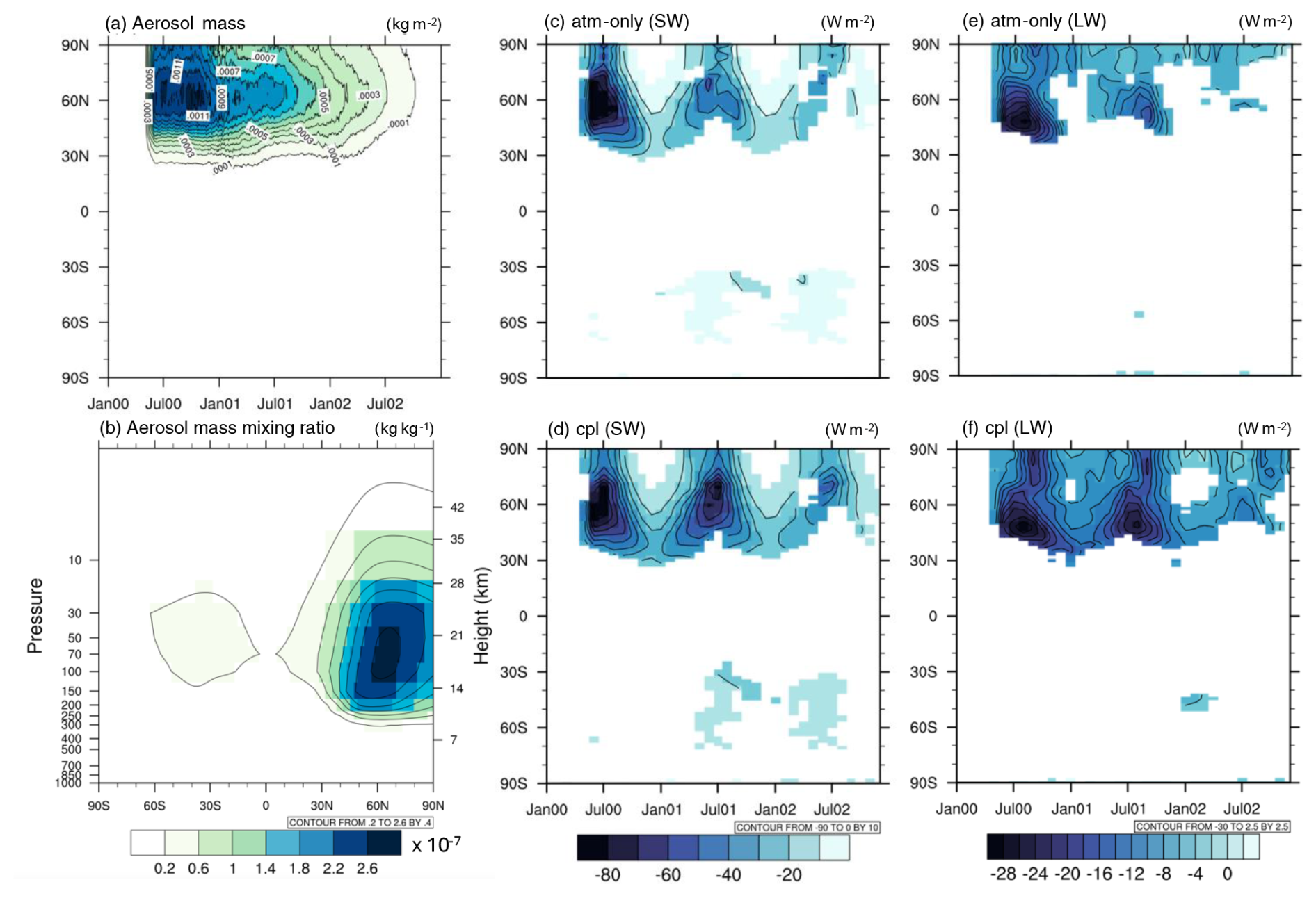
Figure 2 (a) Average aerosol column mass time evolution in kg m⁻² and (b) pressure vs. latitude slice of the prescribed aerosol dry mass mixing ratio in kg kg⁻¹ (3-year average). Aerosol mass is the same in the cpl and atm-only experiments. Panels (c) and (d) show the time evolution of the net SW flux (downward) anomaly at the top of the atmosphere, and panels (e) and (f) show the same but for net LW flux anomaly, resulting from the volcanic aerosol mass, in (c) atm-only and (d) cpl, where colored areas indicate 99 % significance compared to the control experiment according to a Student t test.

LW anomalies also show seasonal evolution with stronger LW flux at mid-latitudes compared to at high latitudes during summer that continues into the winter season and remains significant throughout most of these 3 years. During winter, the LW anomalies are present at high latitudes where the SW anomalies are absent. The latitudinal bands of radiative flux anomalies correspond to the maximum values of the aerosol mass between 60 and 70° N, with the total aerosol mass of 14.04 Tg being largely confined north of 45° N (Fig. 2a–b). Overall, the idealized radiative forcing is largely bounded by the NH extratropics, with the exception of a slight but significant increase around 30–60° S in the second and third summer (Fig. 2c–d) that is visible at around 14–15 km a.s.l. (Fig. 2b). This occurs due to spatial features in the Neely et al. (2016) aerosol forcing that we use for scaling, where a slight aerosol increase occurs at lower latitudes, although this is not detectable when the aerosol mass is averaged through the atmospheric column with respect to time (Fig. 2a). We also detect a slight difference in the LW and SW fluxes that arises from differences in high cloud cover between atm-only and cpl, where cpl shows a decrease in high cloud cover in the northern high latitudes, compared to atm-only (not shown).

3.2 Stratospheric response

The strong seasonality in the LW perturbations described above also characterizes stratospheric temperatures, where a strong increase in the zonally averaged temperature at 50 hPa (T50) is detected north of 30° N during post-eruption summers in both experiments (Fig. 3a and b). This summer warming is followed by a net cooling of the polar stratosphere in the first winter seen for both cpl and atm-only. A clear difference in the T50 response in the two experiments is seen in winter 2, where cpl yields warming over polar latitudes while atm-only yields cooling (Fig. 3a, b). This reveals the intra-seasonal dynamical effects in the cpl experiment beyond the direct radiative response as we will see later on. The contrasting temperature response is accompanied by an opposite response in the zonal-mean zonal winds at 10 hPa (U10) between 70 and 80° N. This U10 response is an indicator of the state of the polar vortex, where a polar vortex weakening is detected in winter 2 for cpl but a strengthening is detected for atm-only (Fig. 3c–d). Figure 3c–d do show a large ensemble spread in the zonal-mean U10 winter response that is evidence of a low signal-to-noise ratio. While the first winter in cpl and the first two in atm-only show little statistical significance according to a Kolmogorov–Smirnov test, this significance does increase for winter 2 in the cpl experiment. We also see this weakening in the zonal-mean U50, also showing stronger significance during winter (Fig. S3 in the Supplement), but not as clearly as in the zonal-mean U10. However, for consistency we will mainly be focusing on the U50 response in the following section, where this response is clear over the NH polar cap. The difference between cpl and atm-only will be the focus in the following sections.

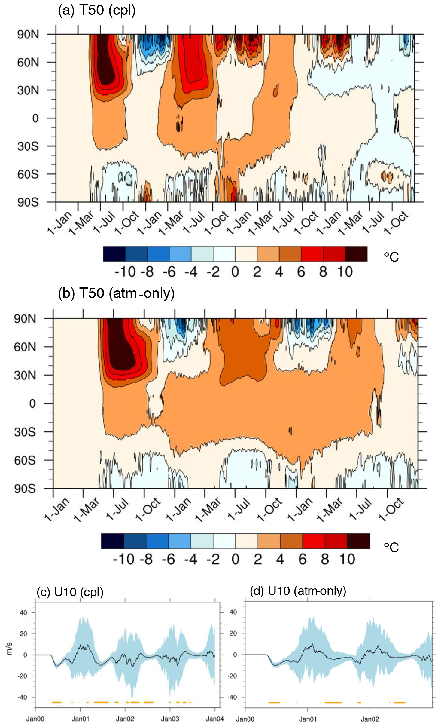
Figure 3 (a, b) Latitude versus time response of T50 anomalies over the investigated period in (a) cpl and (b) atm-only (note the different timescale). Contours are significant at 95 % confidence intervals according to a Student t test. (c, d) Stratospheric polar vortex response shown as the zonal-mean U10 anomalies between 70 and 80° N for (c) cpl and (d) atm-only. Black lines show the ensemble mean anomalies, and blue shadings show the ensemble ±2 standard deviation anomaly range. Orange markers indicate when the difference between perturbed and unperturbed experiments becomes significant (p < 0.05) according to a Kolmogorov–Smirnov test.

3.2.1 First post-eruption winter

In the cpl experiment, the polar vortex strengthening in winter 1 is associated with extensive anomalies in temperature and zonal wind at 50 hPa (Fig. 4a). The anomalous temperature pattern consists of cooling at high latitudes and into the mid-latitudes over the Atlantic, as well as warming over large swaths of the subtropics (to 20° N) and into the mid-latitudes over the Pacific. This temperature pattern is also identified in the zonal-mean T50 (Fig. 3b). Similarly, the zonal wind weakens into the mid-latitudes over the Pacific, while it is stronger in mid- to high latitudes over the Atlantic. The strong upward EP flux (black arrows) is an indicator of the direction of propagated waves originating at the surface around the mid-latitudes, where the horizontal and vertical EP flux components are proportional to the eddy momentum and heat flux, respectively (Fig. 4d). A convergence (negative divergence, dashed red contours) in the EP flux that acts to weaken the tropospheric westerlies is detected in the upper troposphere (Figs. 4d and S2). However, the EP flux and its convergence within the stratosphere does not appear to impact the stratospheric mean flow and the polar vortex. Therefore, the local heating due to the volcanic aerosols and the associated increase in the meridional temperature gradient in the stratosphere appear to dominate the response of the polar vortex via thermal wind response, also depicted by the LW anomalies (Fig. 2f). Winter 1 in atm-only shows a thermal wind mechanism at play in the stratosphere similar to the cpl experiment (Figs. 5a and 4a, respectively). In that case, less obvious tropospheric influences are detected, due to a lack of forced surface cooling, as seen in the limited anomalous upward wave activity detected by the EP flux diagnostics (Fig. 5c).

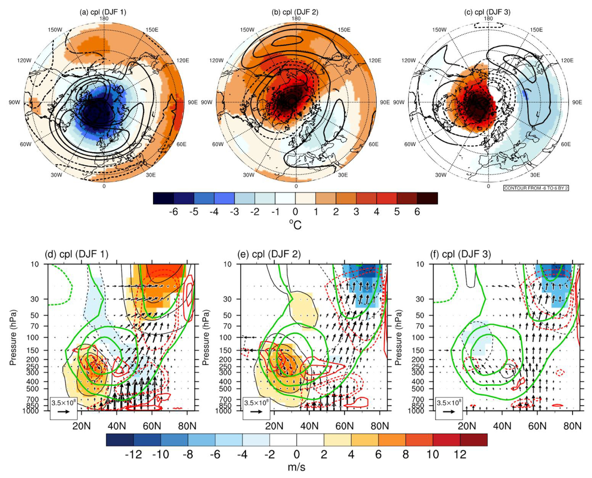
Figure 4 Winter stratospheric response in the cpl experiment. (a–c) U50 (contours) and T50 (shading: red indicates warming and blue indicates cooling) response for winters 1–3, respectively. (d–f) EP flux (arrows) and divergence (red contours) response, along with zonal-mean zonal wind response (black contours and shading: red indicates strengthening and blue indicates weakening) and climatology (green contours) in winters 1–3, respectively. Contours and color-shaded areas indicate 95 % significance according to a Student t test. Only vectors that are significant at the 95 % confidence interval are shown.

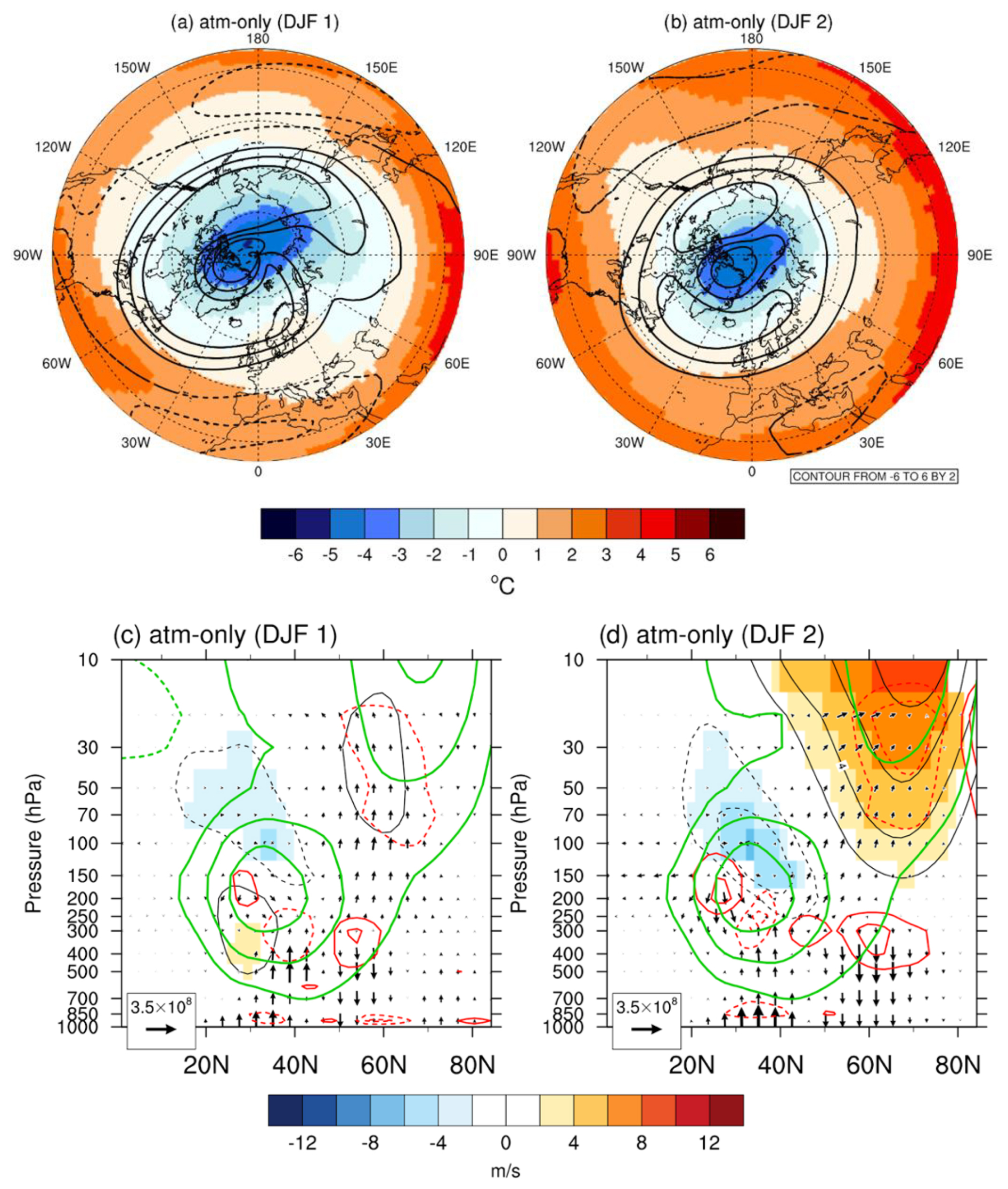
Figure 5 The same as Fig. 4 but for the atm-only experiment. (a–b) Zonal wind (contours) and temperature (shading) response at 50 hPa for winter 1 and winter 2, respectively. (c–d) EP flux (arrows) and divergence (red contours) response along with zonal-mean zonal wind (black contours) and pure climatology (green contours, 2 m) in winters 1–2, respectively. Contours and colored area indicate 95 % significance according to a Student t test.

3.2.2 Second post-eruption winter

A stark difference in the polar vortex response is detected between cpl and atm-only in winter 2. While atm-only exhibits a response similar to winter 1 (Fig. 5b), a significant warming over North America and the North Pacific emerges in cpl along with a weakening of U50 at high latitudes (Fig. 4b), indicating a shift of the polar vortex towards Eurasia. This warming at high latitudes then coincides with a slight LW absorption at high latitudes (Fig. 2f). The U50 weakening is not uniform throughout the longitudes, explaining the lack of response detected in the zonal-mean U50 (Fig. S3), where one needs to go to U10 to get a clear response in the zonal-mean zonal wind (Fig. 3c). An anomalously strong upward propagation of planetary waves persists in the cpl (Fig. 4e), with a stronger upward EP flux now protruding into the stratosphere above 20 hPa, in contrast to winter 1. The upward EP flux and its convergence in the polar stratosphere are evidence of their contribution towards the weakening of the U50 and a general dominance over the effects of thermal forcing by aerosols that have been, at this stage, substantially reduced (Fig. 1).

A similar wave propagation pattern to that identified in the cpl experiment is known to be associated with SSWs. We suspect that the decrease in the T50 difference between mid- and high latitudes can act as a trigger for a weaker polar vortex, in addition to the stratosphere absorbing the upward-propagating waves that is known to cause warming over the polar cap (Kodera et al., 2016; Kretschmer et al., 2018). We will see further evidence of this in the next section.

3.2.3 Third post-eruption winter

The results in this section only refer to the cpl experiment since winter 3 is lacking in atm-only. The SSW-like pattern of winter 2 clearly continues into winter 3, where most of the volcanic aerosols have decreased to such an extent that their radiative impacts no longer dominate. An exception is the confinement of T50 warming over the polar stratosphere (Fig. 4c). Furthermore, anomalous upward propagation of planetary waves continues to persist (Fig. 4f). This upward wave flux in addition to the T50 warming resembles a pattern that behaves much like absorbing SSWs defined by Kodera et al. (2016). To examine this response further, we define SSWs based on the reversal of the zonal-mean zonal winds at 60° N and at 10 hPa between November and March according to the method of Charlton and Polvani (2007).

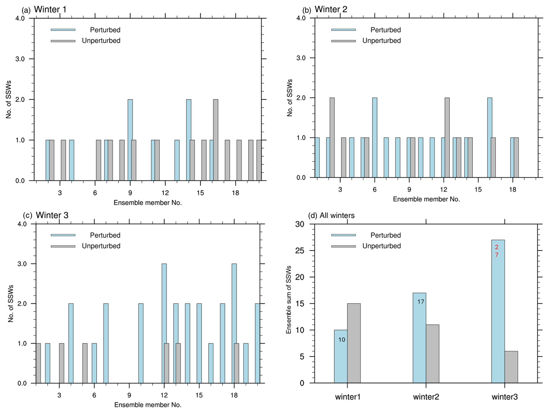
Figure 6 (a–c) The number of SSWs during winters 1–3 for each ensemble member in the cpl experiment and (d) the sum of all SSWs in each experiment for all 20 ensemble members of winters 1–3 for both cpl (light-blue bars) and control (gray bars). The color red indicates 95 % significance according to a two-sided Student t test.

Results from the SSW analysis are presented in Fig. 6. No significant increase in SSWs is found in winter 2, despite the SSW-like pattern detected. This changes in winter 3 when the difference between the perturbed experiment and the unperturbed experiment becomes statistically significant, with 27 SSWs occurring in our forced experiment compared to only 6 in the control experiment. This increase in SSWs agrees well with the U50 and T50 anomalies of winter 3 (Fig. 4c). During winter 2, the warming of the polar stratosphere is as strong as in winter 3 but more spread out into mid-latitudes. These results are also in agreement with the stratospheric Plumb flux in winter 3 (Fig. S1c), where the upward flux is mostly circumpolar between 40 and 60° N, showing further evidence of the SSWs detected.

When comparing the ensemble sum of SSWs in the perturbed and unperturbed experiment using a Kolmogorov–Smirnov test (Fig. 6d), a significant increase in the number of SSWs occurs in winter 3 (p = 0.0135). This underlines the generally strong SSW response occurring in winter 3, when the fraction of ensemble members having more than one SSW per winter increases to 50 % (10 ensemble members) in winter 3 compared to only 10 % in winters 1–2. Of these 10 ensemble members, two members show three SSWs per winter that can be considered highly unlikely based on historical records. Although winters with more than one SSW are considered unusual, examples do exist in the observational record of multiple SSWs in one winter, like the winter of 1998–1999 and 2009–2010 (Kodera et al., 2016; Ineson et al., 2023, respectively).

To better understand the cpl SSW response, we also did an SSW analysis on atm-only (Fig. S7) where 50 %–75 % fewer SSWs were detected in the perturbed simulation compared to the unperturbed one. Such a response should not be unexpected during the forced polar vortex strengthening as detected in atm-only (see Fig. 5). Furthermore, only single SSWs per winter were detected in all 20 ensemble members of the perturbed simulation, while two (one) ensemble member(s) detected double SSWs per winter 1 (winter 2) in the unperturbed simulation. Although these results do suggest an increase in the number of SSWs in the cpl simulation, internal variability is large, and the frequency of SSWs fluctuates substantially between the three winters in the unperturbed simulation.

We explored the impact of the ensemble size for the ensemble spread of two key diagnostics of our mechanism, namely U10 and SSW, calculated as the standard deviation of post-eruption paired anomalies for the first three post-eruption winters (Fig. S8). Winter 3 produces a larger spread than winters 1 and 2, indicative of a less constrained forced response, which is especially evident for ensemble sizes larger than 15. Accordingly, this analysis suggests that much larger ensembles are needed to confidently demonstrate the significance of the SSW response (i.e., to provide signals not encompassing the value of zero within uncertainty).

According to the above, the evolution in cpl from winter 1 to winter 3 can be summarized as follows. In the first winter, the thermal forcing appears to be stronger than the upward wave flux because of the large amount of aerosols present, thereby dominating the response that causes the polar vortex strengthening and the inclusion of cold polar air within. In the second winter, the thermal forcing from the volcanic aerosols at mid-latitudes has decreased to where it is now mostly confined to higher latitudes as seen in both the LW flux and T50 (Figs. 2f and 3b). We suspect that in addition to the aerosol decrease, this slight decrease in the temperature difference between high and mid-latitudes allows the strong upward wave flux to dominate and enter the upper stratosphere. There in the stratosphere the waves are absorbed, which causes further warming over the polar cap, in addition to weakening the zonal stratospheric winds (Figs. 5b and 4b). This upward wave flux and weaker winds continue into the third winter, where winter 2 potentially acts as a precursor, allowing for SSWs to develop more frequently as detected in the T50 warming that is now confined over the polar cap (Figs. 4c and 5c, respectively). The SSW development is also evident in both U10 and U50 and T50 time series (Figs. 3c and S3a–b, respectively), where peak T50 warming occurs late in winter 3. The expected absence of a surface response is obvious in our atm-only experiment, where the basic physical mechanism, via the thermal wind balance due to radiative heating, dominates the atmospheric circulation response in the first two post-eruption winters. The strong stratospheric polar vortex then isolates the cold air over the polar regions (Fig. 5a–b) as is the case in winter 1 in the cpl experiment (Fig. 4a).

3.3 Tropospheric response

What is it then that drives this polar vortex weakening and the SSW response in the cpl experiment? To examine in more detail the origin of the upward wave fluxes in winters 2 and 3 of the cpl experiment that causes the detected polar vortex weakening and the SSWs, we now turn our attention towards the troposphere.

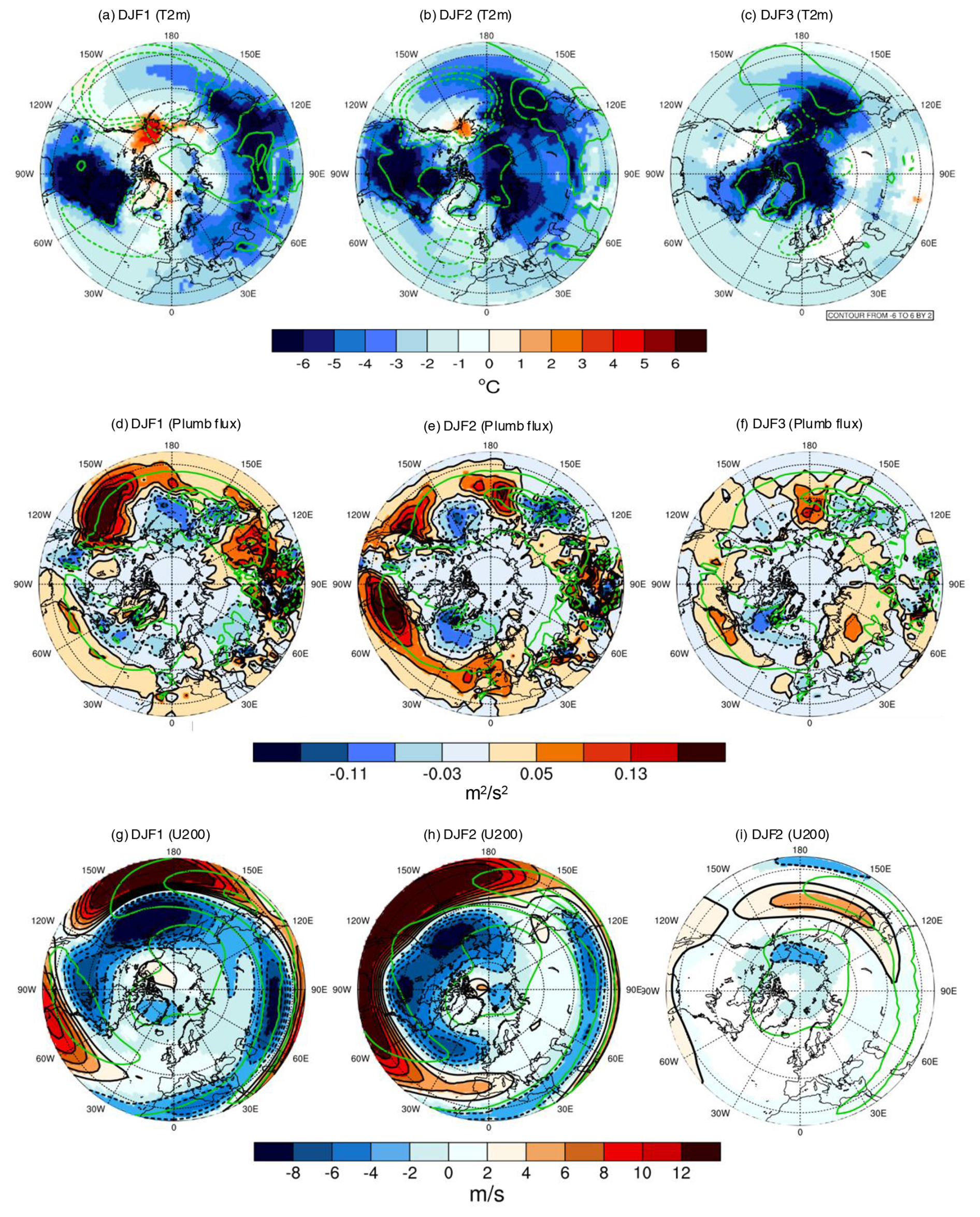
Figure 7 (a–c) 2 m air temperature (°C) in cpl (color) and sea-level pressure (green contours) anomalies for winters 1–3. (d–f) The vertical component of the Plumb flux (m² s⁻²) at 850 hPa in cpl, and the climatology as green contours from −8 to 12 in increments of 2 for winters 1–3. (g–i) 200 hPa zonal wind (m s⁻¹) anomalies in cpl, and the climatology as green contours from −0.15 to 0.15 in increments of 0.04 for winters 1–3. Contours and colored areas indicate significance at the 95 % confidence interval according to a Student t test.

We begin by comparing the response of T_2 m and the vertical Plumb flux at 850 and 200 hPa zonal wind in cpl (Fig. 7) and in atm-only (Fig. 8).

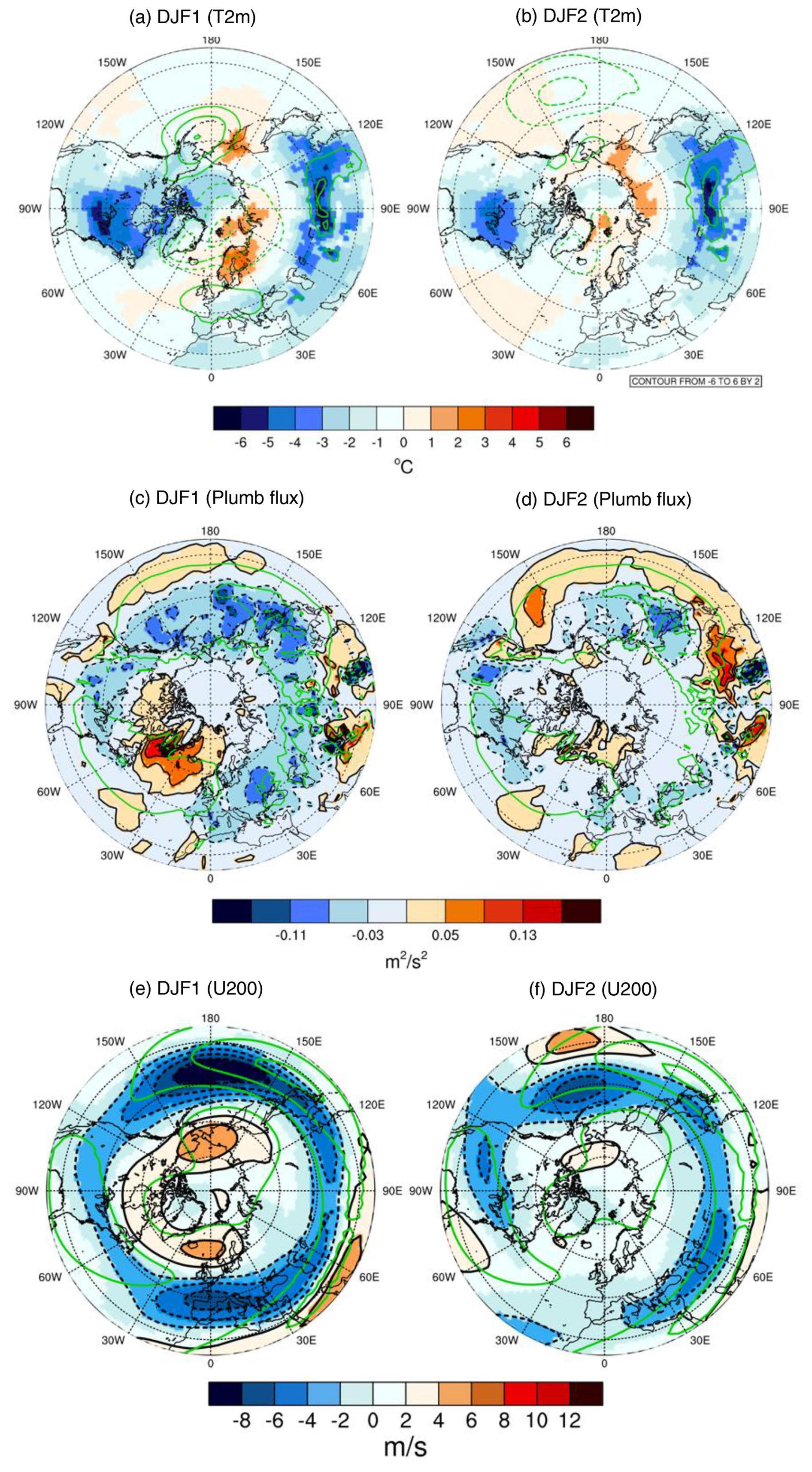
Figure 8 The same as Fig. 7​​​​​​​ but for the first two winters in atm-only. Contours and shaded areas indicate significance at the 95 % confidence interval according to a Student t test.

As a response to the decrease in SW flux following the eruption, extensive and heterogeneous cooling is identified in the T_2 m anomalies in winters 1–3 (1–2 for atm-only) over latitude bands that contain the most significant SW flux decrease (Figs. 2d, 7a–c and 8a–b). The strongest cooling occurs over northeastern North America and along the Asian mid-latitudes in winter 1, with much larger amplitude in cpl than in atm-only (Fig. 7a versus Fig. 8a). In cpl, a significant cooling is identified in the SST (Fig. S5), extending the area of negative T_2 m anomalies towards the ocean, in particular over the northwestern North Pacific in winter 1 (Fig. 7a). There it progresses from an initial preferential surface cooling over the mid-latitudes in winter 1 to a later cooling of polar regions in winter 3 (Fig. 7c). In atm-only, the surface response is hampered over the ocean by the experimental design, and T_2 m anomalies are therefore confined to landmasses, yielding an overall much weaker temperature response compared to cpl (Fig. 8a–b).

The vertical component of the Plumb flux at 850 hPa (Fig. 7d–f) allows us to locate the origins of the upward EP flux in cpl (Fig. 4d–f). It is strongest over the northeastern part of the Pacific Ocean (off the west coast of North America) in winter 1, where it continues up into the lower stratosphere at 150 hPa (see Fig. S1a). In winter 2, the Plumb flux has decreased in the North Pacific and increased over the North Atlantic and Siberia, pointing to a possible influence of the change in the land–sea temperature contrast (Fig. 7e). In addition to this upward flux, we also detect a downward wave flux over both the Aleutian and Greenland regions at 850 hPa and over a large area south of 45° N at 150 hPa (Fig. S1b). This downward Plumb flux is evidence of changes in the planetary wave structure, where wave reflection occurs due to the sudden weakening of the zonal winds identified in the U10 (Fig. 3a). In winter 3, the Plumb flux now dominates at both 850 (seen in Fig. 7f) and 150 hPa (Fig. S1c), where it encircles the polar stratosphere north of 60° N. In line with the weak EP flux response shown in Fig. 5, the Plumb flux anomalies are generally weak in atm-only compared to cpl for both winter 1 and winter 2 (Fig. 8c–d).

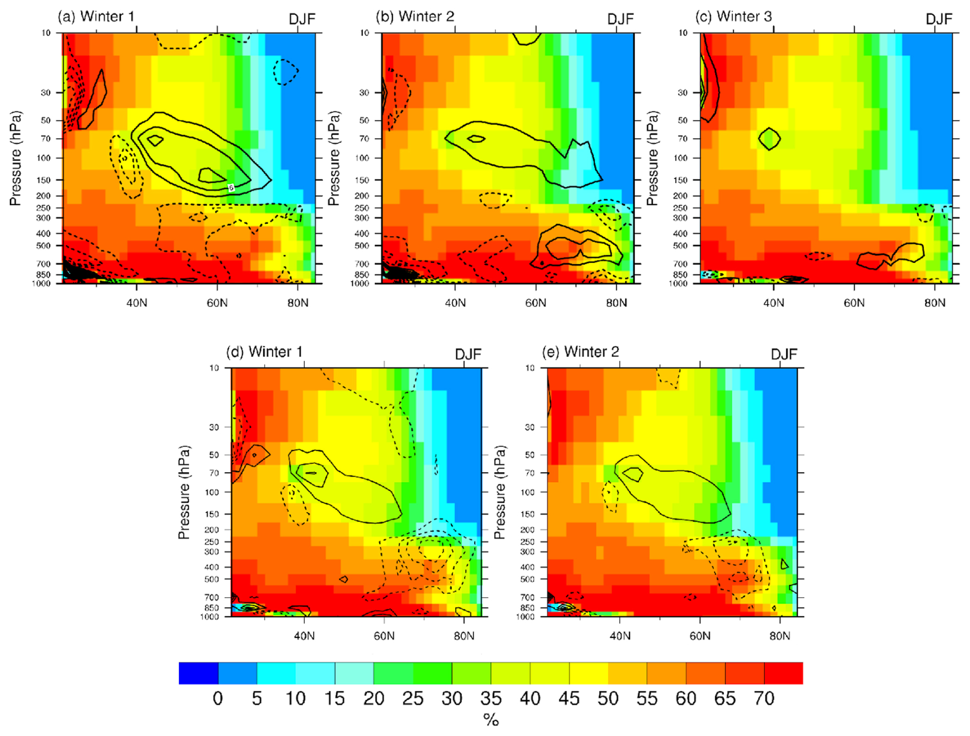
Figure 9 Probability (%) of favorable propagation conditions for large-scale stationary Rossby waves (zonal and meridional wavenumbers 1, 2, and 3) as a function of latitude and pressure levels (shading). Contours are from −30 to 30 in increments of 3 and show the probability of favorable conditions in the long summer versus control. (a–c) Winters 1–3 in cpl. (d–e) Winters 1–2 atm-only.

Since upward wave activity depends on wave–mean-flow interactions, several factors are at play to explain the strong response in cpl vs. atm-only. First, the change in zonal flow is substantially different between the two pairs of experiments, as shown by the U200 anomalies (Figs. 7g–i and 8e–f). In the first two winters we observe an intense deepening of the Aleutian low in cpl (Fig. 7a–b), associated with a large equatorward shift of the subtropical jet over the North Pacific (Fig. 7g–h, also seen in the zonal-mean averages of Fig. 4). The change in zonal flow is not as large in atm-only, where there is a general decrease of U200 on the poleward side of the subtropical jets, rather than a marked equatorward shift as in cpl. This further emphasizes that amplified surface coupling when the ocean is coupled to the atmosphere has a dramatic impact on the amplitude of the tropospheric response. Because the zonal flow acts as a waveguide for large-scale planetary waves, we expect changes in upward wave propagation in the stratosphere. To measure how waveguides change, we compute the probability of favorable propagation conditions for large-scale stationary waves (Fig. 9). This is averaged for zonal wave numbers k = 1, 2, and 3 and meridional wave numbers l = 1, 2, and 3, as a function of pressure and latitude (see Sect. 2 for more details). Areas of high probability show where large-scale waves preferentially propagate, while low-probability regions indicate where linear wave propagation is hampered. Generally, the mid-latitude troposphere is more favorable for wave propagation than the high latitudes and the stratosphere, consistent with the tendency for stationary waves to propagate upwards and to be deflected towards the Equator in climatology. After injection of the volcanic forcing, both cpl and atm-only exhibit an increase in the probability for wave propagation between 40 and 60° N in the lower stratosphere during winter 1 and 2, but the responses in the troposphere are markedly different. In atm-only, wave propagation is inhibited in the free troposphere north of 60° N for both winter 1 and winter 2 (Fig. 9d–e), which is consistent with the EP flux anomalies of Fig. 5. This response is absent from cpl during winter 1 (Fig. 9a) and opposite during winter 2 when an increase of favorable conditions for wave propagation is diagnosed (Fig. 9b). We also see that the waveguide has been greatly reduced in the subtropical troposphere in cpl winters 1–2, which favor large-scale waves to be redirected towards the pole. This increase in favorable conditions for wave propagation in the troposphere between 60 and 80° N persists during winter 3 in cpl (Fig. 9c), which is a partial and the most likely explanation for enhanced upward wave propagation in the stratosphere described in Fig. 4f.

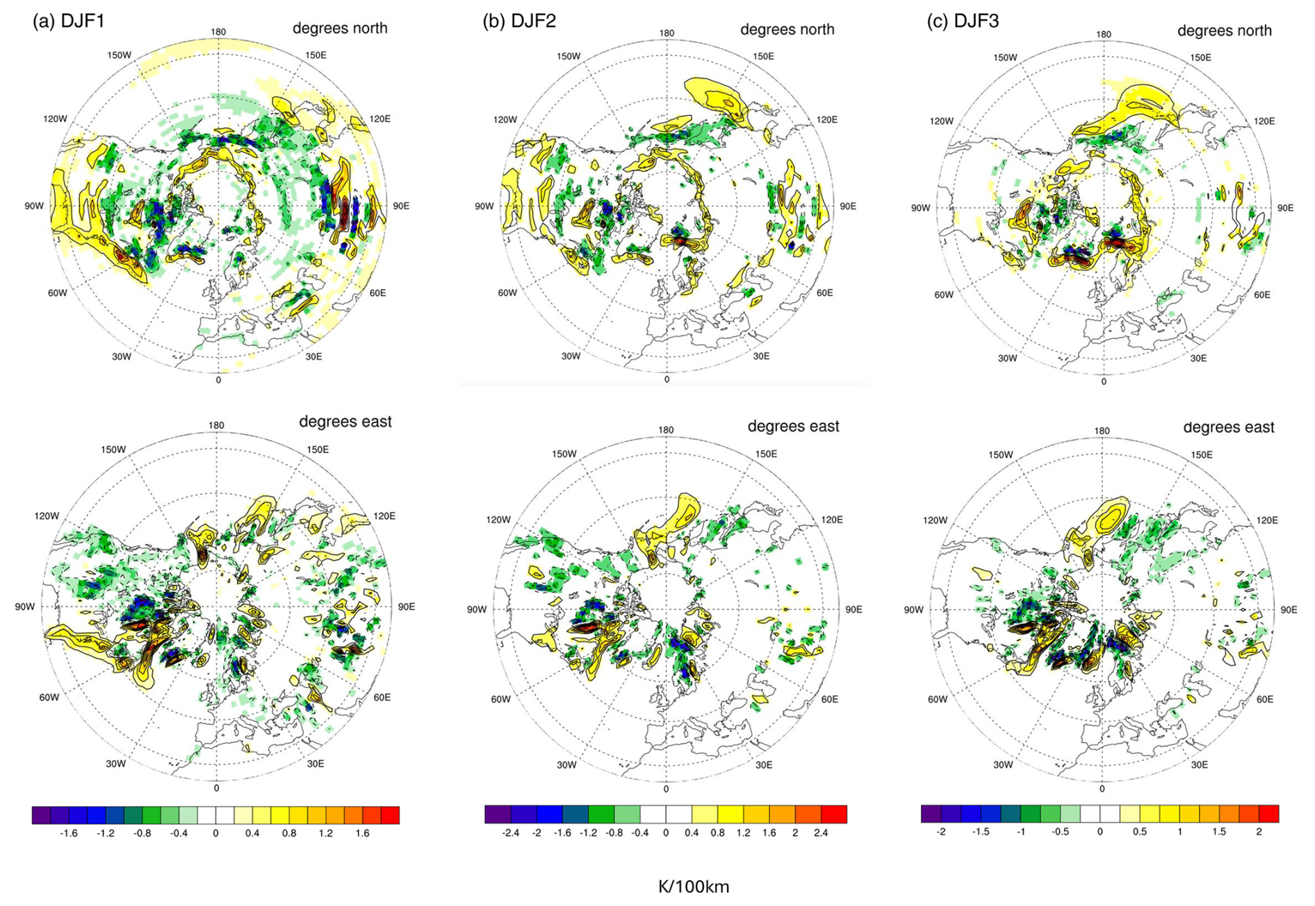
Figure 10 (a–c) The zonal (degrees north) and meridional (degrees east) T_2 m gradient anomalies (perturbed minus unperturbed) for winters 1–3. Contours indicate 95 % significance according to a Student t test. Note the different color bar for each winter.

In cpl winter 3, when the cooling is reduced in the NH mid-latitudes and has migrated towards the polar regions (also evident in SST; see Fig. 5S), the amplitude of the 850 hPa upward Plumb flux anomalies decreases compared to previous winters (Fig. 7f). This suggests that the mid-latitude spatiotemporal cooling pattern plays a part in the strong wave activity detected near the surface. This can be revealed by computing the T_2 m gradient (T_grad​​​​​​​), where strong land–sea temperature gradients are known for their ability to influence atmospheric wave activity (Hoskins and Valdes, 1990; Brayshaw et al., 2009; He et al., 2014; Wake, 2014; Portal et al., 2022). Figure 10a shows sharp significant changes in the meridional gradient that encircles 45° N in winter 1, with positive (negative) gradient anomalies occurring south (north) of 45° N. In winter 2 we still see the gradient present at 45° N but now located over North America and the North Pacific. Winter 3 mostly reveals regional anomalies in the Barents–Kara, Greenland–Iceland, and the North Pacific regions (Fig. 10b–c), occurring over areas of significant sea-ice increase (not shown). The sharp T_grad change in winter 1 (Fig. 10a) is followed by a reduction of land–sea temperature contrast over eastern Canada and the US in winter 2 (Fig. 10b). This is a known cause of planetary wave enhancement (Portal et al., 2022) and could provide an explanation for the strong surface upward wave flux detected in the second and third post-volcanic winters (Fig. 7e–f). Both the zonal and meridional T_grad components show an increase in the northern part of Alaska that coincides with the region of T_2 m warming over the Aleutian and Alaska region (Fig. 7a) and the strong upward Plumb flux (Fig. 7d). This warming, in addition to the strong continental cooling over the northeastern US and the general decrease in T_grad spanning from the middle to northern part of North America, might influence this strong Plumb flux anomaly in the North Pacific. Notably, sea-ice extent increases around East Siberia, extending into the Chukchi Sea (not shown) and highlighting the potential influence of sea-ice variability on T_grad and upward Plumb flux anomalies in the area.

Plotting the average T_grad for various regions against the average number of SSWs for winters 1–3 (Fig. S6), we do see that the strongest T_grad reduction occurs over the northeastern US in the second winter. This is in agreement with the upward Plumb flux over the same region, serving as further evidence for its contribution to the upward EP flux in winter 2. This T_grad reduction continues into the third winter, where we also detected a reduction in the upward Plumb flux over the same area (Fig. 7f). Looking towards the Barents Sea, a clear spatial difference emerges compared to the northeastern US, where a clear T_grad increase occurs in winter 3 and is related to the SSWs. In general, fewer changes are detected between winters in northwestern North America and the North Pacific, reflecting the confined cooling over higher latitudes in winter 3 associated with the SSWs.

To complete our assessment of the tropospheric response, we examine if eddies play a role in the cpl polar vortex response and the anomalous upward EP flux (Fig. 4a–f) as well as SSWs detected in winter 3 by following Smith et al. (2022) (see Methods). This is done for both perturbed (red) and unperturbed (blue) experiments in cpl and atm-only (Fig. S4). We see an increase in perturbed eddy feedback at around 40–70° N both for winter 1 in cpl and winters 1–2 in atm-only during the polar vortex strengthening (Fig. S4). However, the role of eddies in the polar vortex weakening in winters 2–3 is unclear, especially considering the eddy feedback increase of the control run in winter 2 (Fig. S4b). In general, these results suggest that the signal-to-noise ratio is too small to identify a role for eddy feedback in our experiments.

4 Discussion

Our two sets of coupled ocean–atmosphere (cpl) and atmosphere-only (atm-only) experiments examine the large-scale climate response to an idealized, long-lasting NH eruption, where their differences give us valuable insight into the volcanically forced mechanisms at play within the coupled climate system in CESM1. Specifically, we analyzed the first three winters of the cpl experiment and used the first two winters of atm-only as a comparison to investigate the dynamics that govern the post-eruption stratospheric polar vortex and the associated surface response.

Results from the cpl experiment show a similar response in the first winter to that in the two winters of atm-only, with a strengthening of the zonal winds resulting from an aerosol-induced sharp temperature gradient between the mid-latitudes and the pole (Figs. 4a and 5a). We show that this zonal wind strengthening is not affected by the detected strong upward EP flux, where the LW flux (Fig. 2e–f) supports our conclusions that the polar vortex strengthening is induced by the thermal wind balance. A distinct change to this pattern emerges in cpl winter 2, where we detect an SSW-like pattern, with strong negative anomalies emerging in the polar U50 winds and a warming in the T50 field (Fig. 4b). We also detect an LW absorption at high latitudes which is absent at mid-latitudes, where this T50 warming is evidence of the potential role of a decreased temperature gradient in the identified polar vortex weakening. Furthermore, the upward wave-activity flux from the troposphere into the stratosphere and the T50 warming indicate absorption of upward-propagating waves into the stratosphere that causes this warming and weakening of U10 winds over the polar cap. This pattern is known to be related to SSWs (Kretschmer et al., 2018; Kodera et al., 2016), agreeing with our results in winter 3, where an increase in the occurrence of SSWs is detected. The strong upward EP flux greatly depends on ocean–atmosphere coupling originating in the surface cooling, in addition to the changes in upper tropospheric zonal flow. This further contributes to the upward EP flux from the troposphere into the stratosphere that eventually leads to polar vortex weakening and enhanced SSWs.

Although the above coincides with a positive (negative) eddy feedback in the first (second) winter that could in theory play a role in sustaining the strengthening (weakening) of the polar vortex, our eddy feedback results indicate a low signal-to-noise ratio, where further studies with additional ensemble members would be required to confirm their role in the forced response. We also note that Smith et al. (2022) identified CESM1 SC-WACCM as having one of the weakest eddy feedbacks of the 16 models they investigated, so the response of the eddy feedback may be more significant in other models. Similar to the eddy feedback, a low signal-to-noise ratio is also evident in the SSW analysis. However, the response we detect in the U50 and T50 fields is strong compared to the unperturbed simulation, where the SSWs provide an explanation in agreement with the patterns detected. Furthermore, the SSW analysis for atm-only and the ensemble size test (Figs. S7 and S8, respectively) both suggest the presence of a robust signal for winter 3 despite the noisy polar vortex and the limited ensemble size. We also see that the large decrease in SSWs in the perturbed simulation of atm-only (when compared to unperturbed) is consistent with the detected polar vortex strengthening. This further supports the significance of the signal we detect in cpl winter 3 compared to the background noise. In addition, all winters examined, in both cpl and atm-only, showed that there is up to a 15 % chance of getting more than one SSW per winter in all ensemble members. This is not far from Ineson et al. (2023), who identified a double event once every 9 years in a 66-year ERA5 record. The exception is cpl winter 3, which is also the only winter that has three SSWs, with the average SSW occurrence also being the only winter above 1 (1.17), while all other winters span between 0.15–0.85 per winter. A similar NH high-latitude eruption has not taken place during the observational period, so we have no comparison. Also, to the best of our knowledge, a similar high-latitude sulfur injection study has not been performed before. Therefore, it is difficult to say at this stage if such a response is realistic or not, but in general more than two SSWs per winter can be considered exceptional yet plausible, as is also the case for our idealized eruption.

Bittner et al. (2016b) identified an opposite response driven by a similar underlying mechanism, when compared to our cpl response in winters 2–3 (Fig. 4), following a Tambora-like eruption where a strengthening of the polar vortex due to less wave breaking at high latitudes was considered to be an indirect effect associated with a changes in planetary wave propagation. Since the volcanic aerosols in our experiments have declined extensively in the third winter, making the aerosol thermal forcing a limited factor, we cannot rule out similar indirect effects where changes in wave propagation lead to an increase in wave breaking at high latitudes and hence the increase in SSWs.

While not directly comparable to our study but still providing an important analog, Muthers et al. (2016) identified an average increase in the number of SSWs during a 30-year (constant) decrease in solar radiation in line with our significant increase in SSWs in winter 3. Our results do support the findings of Sjolte et al. (2021), where the stratospheric temperature gradient does not appear to play a major role in the polar vortex weakening we identify, while the upward wave flux does.

The strong surface cooling detected in Fig. 7 is a well-known caveat in CMIP5 models (including CESM1) (Driscoll et al., 2012; Chylek et al., 2020) and is clearly detected in our coupled simulations. Since our results indicate the dominant role of the volcanically induced stratospheric thermal wind response that causes the polar vortex strengthening, the cooling does not appear to impact the response identified in winter 1. This is also revealed by the EP flux. The same cannot be said about winters 2–3, where our results indicate that the exaggerated spatiotemporal T_2 m pattern might explain the strong upward wave flux and the associated stratospheric response. Interestingly, a slight difference between atm-only and cpl is detected in both the LW flux and the SW flux and is caused by a strong significant decrease in high cloud cover in the cpl simulation (not shown). This cloud cover decrease, especially at mid- to high latitudes, agrees with the increased LW fluxes at higher latitudes, in addition to the decrease in SW flux and the associated surface cooling. This raises a question regarding the role of forced surface processes in these high cloud changes, which we leave open for further studies.

As mentioned in the Methods section, we assume a lifetime of volcanic aerosols at 65° N similar to at 45° N. When considering the e-folding time in Toohey et al. (2019), a substantial aerosol decrease of about 43 % occurs at 17 km (a.s.l.​​​​​​​) for an eruption at 60° compared to at 0°. However, since our experiment assumes a constant stratospheric injection over 5 months with the aim of simulating a long-lasting, HL eruption compared to a single injection at low latitudes, the difference in the e-folding time between low and high latitudes would be expected to decrease. Using CESM2-WACCM6 with interactive chemistry, Zhuo et al. (2024) identified that although an eruption at 64° N did have a shorter aerosol lifetime compared to one at 15° N, it leads to stronger volcanic forcing over the NH extratropics. In addition, one of their conclusions was that different duration and intensity of both tropical and NH extratropical eruptions can lead to different results, stressing that our 6-month-long stratospheric sulfate aerosol enhancement is not directly comparable with volcanic eruptions of shorter duration. Although the aerosol lifetime in our experiment might be exaggerated into the third year, our results do indicate that the polar vortex weakening in winter 2 appears to act as a trigger for further weakening that eventually leads to SSWs in winter 3. In order to increase confidence in such a delayed link, additional sensitivity simulations are required, which we leave for future studies.

Unlike our eruption simulated using a version of WACCM4, where the chemistry is prescribed, natural volcanic eruptions can contain various chemical compounds that impact the formation and the lifetime of sulfate aerosols as well as affect the atmospheric circulation via, e.g., ozone depletion, like halogens are known to do. More advanced versions as well as models that include interactive chemistry are thus important to reveal in more detail the chemistry–climate interactions that occur in the natural world (Clyne et al., 2021; Case et al., 2023; Fuglestvedt et al., 2024). Thus, our idealized experiment can be considered primitive in the sense that it only considers sulfate aerosols but sufficient when focusing on answering questions on the basic mechanism that such eruptions can initiate. Another important aspect that we do not focus on in our study is the role of different initial conditions on the forced climate response, where initial atmospheric and climate conditions, including, e.g., the stability of the polar vortex, control the lifetime and distribution of the volcanic aerosols as well as the forced dynamic climate response (Zanchettin et al., 2019; Weierbach et al., 2023; Zhuo et al., 2024; Fuglestvedt et al., 2024). An exception is our assessment of how the easterly phase and westerly phase of the QBO affect our results, where we compared ensemble members showing the easterly phase with the westerly ones to test if the U50 and T50 response patterns would be different. They were not: both phases showed a weakening of the U50, although the zonal winds were more confined and consistent over the higher latitudes of the NH during the easterly phase (not shown). The difference in the number of ensemble members used for these calculations could of course impact the statistics of this test of ours but not the overall pattern detected.

CESM2-WACCM6 has obvious improvements when compared to CESM1-WACCM4 (see e.g., Gettelman et al., 2019, Danabasoglu et al., 2020), among them being an interactive QBO as well as having a slightly higher frequency of SSW occurrence (Holland et al., 2024). Nonetheless, CESM1-WACCM4 has comparable transient climate response to CESM2 as well as the ability to capture the general physical mechanism occurring within the climate system as identified in various recent studies (Danabasoglu et al., 2020; Zhang et al., 2018; Elsbury et al., 2021b; Peings et al., 2023; Ding et al., 2023; Yu et al., 2024).

5 Conclusions

Through comparison of the cpl and atm-only simulations, our results clearly demonstrate the important role of ocean–atmosphere coupling in the stratospheric response to enhancements of the stratospheric sulfate aerosol layer at higher NH latitudes. We see that this aerosol enhancement layer triggers two competing mechanisms in the first three winters.

• i.

  Winter 1. The stratospheric polar vortex strengthening is triggered by stratospheric aerosol thermal forcing via thermal wind balance. This response is not influenced by the strong upward wave flux identified, originating in the forced surface cooling and changes in tropospheric circulation, and provides strong evidence of two mechanisms that are competing simultaneously – a top-down and a bottom-up mechanism, where the top-down mechanism dominates the response.

• ii.

  Winter 2. The upward wave flux is absorbed in the stratosphere, which causes a warming over the polar cap and a polar vortex weakening. This pattern is similar to SSWs, although its occurrence is not significant. Here the bottom-up mechanism dominates.

• iii.

  Winter 3. The persistence of the upward wave flux continuing into the third winter leads to an increase in SSWs with warming now confined over the polar cap, again demonstrating the dominating bottom-up mechanism as in winter 2.

It is clear from our results that the strong surface cooling following the HL sulfate aerosol injection causes dramatic changes in tropospheric circulation. These changes further modify atmospheric waveguides where we detect an increase in propagation of planetary waves in the lower stratosphere occurring at higher latitudes. Although we do find similarities in the eddy feedback when compared to the general climate signal that we identify, such as the decrease in eddy feedback in winter 1 potentially sustaining the polar vortex strengthening, we emphasize its weak signal. At the same time we encourage further studies on this subject, especially concerning the lack of published comparison studies regarding both high- and low-latitude volcanic eruptions and SSWs. Ideally such studies would include the latest model generations in addition to observational datasets. They should also consider the impact of different climate realizations and the eruption magnitude on the forced response. Furthermore, these results highlight the importance of including high-latitude volcanic forcing simulations of various lengths and/or magnitudes in projects such as VolMIP, especially considering the current volcanic unrest and increased activity in some of the major volcanic systems in Iceland.