Estimation of the radiation budget during MOSAiC based on ground-based and satellite remote sensing observations

An accurate representation of the radiation budget is essential for investigating the impact of clouds on the climate system, especially in the Arctic, an environment highly sensitive to complex and rapid environmental changes. In this study, we analyse a unique dataset of observations from the central Arctic made during the MOSAiC (Multidisciplinary drifting Observatory for the Study of Arctic Climate) expedition in conjunction with state-of-the-art satellite products from CERES (Clouds and the Earth's Radiant Energy System) to investigate the radiative effect of clouds and radiative closure at the surface and the top of the atmosphere (TOA). We perform a series of radiative transfer simulations using derived cloud macro- and microphysical properties as inputs to the simulations for the entire MOSAiC period, comparing our results to collocated satellite products and ice-floe observations. The radiative closure biases were generally within the instrumental uncertainty, indicating that the simulations are sufficiently accurate to reproduce the radiation budget during MOSAiC. Comparisons of the simulated radiation budget relative to CERES show similar values in the terrestrial flux but relatively large differences in the solar flux, which are attributed to a lower surface albedo and a possible underestimation of atmospheric opacity by CERES. While the simulation results were consistent with the observations, more detailed analyses reveal an overestimation of simulated cloud opacity for cases involving geometrically thick ice clouds. In the annual mean, we found that, during the MOSAiC expedition, the presence of clouds leads to a loss of 5.2 W m⁻² of the atmosphere–surface system to space, while the surface gains 25.0 W m⁻² and the atmosphere is cooled by 30.2 W m⁻².

1 Introduction

In recent decades, the Arctic has undergone the most rapid changes in climate on Earth (Serreze and Barry, 2011). Characterised by its unique conditions, the warming in the Arctic region is considered a robust feature of climate change (Meredith et al., 2019). The German (AC)³ project has been established to investigate the mechanisms responsible for this warming (Wendisch et al., 2023). Clouds are important for regulating regional and global climate (Huang et al., 2017; Tan and Storelvmo, 2019; Zib et al., 2012). Understanding the properties and effects of Arctic clouds is thus a key goal of (AC)³ as well as the present paper, as they both respond to and drive climate change in this sensitive environment (Morrison et al., 2012; Kay et al., 2016; Taylor et al., 2022, 2023).

Several efforts have been made over time to improve the quantity and quality of observations of Arctic clouds. A general description of the long-term Arctic stations is presented in Uttal et al. (2016). The stations mentioned in Uttal et al. (2016) have been lead observation sites in further investigating and explaining processes and feedback mechanisms in the Arctic region related to regional processes and transport, the atmosphere, and atmosphere–surface exchanges.

Airborne and shipborne research campaigns have been crucial in collecting atmospheric and surface observations in unexplored regions with limited observations, where processes related to this rapidly changing environment remain elusive (see Table 1 in Wendisch et al., 2019). In addition, the Multidisciplinary drifting Observatory for the Study of Arctic Climate (MOSAiC) expedition, conducted from October 2019 to September 2020 (Shupe et al., 2020), aimed to extend the collection of relevant observations related to the Arctic environment. This international collaboration of unprecedented magnitude for an Arctic research cruise provided diverse in situ and remote sensing observations, allowing investigation of various processes related to Arctic clouds and their interactions with the Arctic system (Shupe and Rex, 2022).

Satellite observations of clouds have particular advantages due to their spatial coverage and long duration of service (Stubenrauch et al., 2013; Christensen et al., 2016; Huang et al., 2017). For instance, Eastman and Warren (2010) compared surface cloud observations with datasets from the Advanced Very High Resolution Radiometer (AVHRR) and Television InfraRed Observation Satellite (TIROS) Operational Vertical Sounder (TOVS). Their comparison highlighted the difficulty in finding agreement between both points of view and the additional challenges encountered during the polar night, especially over icy surfaces. Hartmann and Ceppi (2014) observed large changes in the Arctic radiation budget at the top of the atmosphere (TOA) based on CERES (Clouds and the Earth's Radiant Energy System) observations, with trends of −5 and 3 W m⁻² per decade for the shortwave and longwave net fluxes, respectively. Duncan et al. (2020) analyse the trends in the surface radiation budget of the Arctic boreal zone using CERES Energy Balanced and Filled (EBAF) data products from 2001 to 2017 and report a decrease in the reflected solar radiation by 1.3 ± 0.6 W m⁻² per decade and an increase in the outgoing terrestrial radiation by 1.1 ± 0.4 W m⁻² per decade, suggesting a greening of the Arctic tundra. These results are subject to an overall monthly uncertainty of 3 W m⁻² for the solar and terrestrial fluxes (Loeb et al., 2018).

The study by Lelli et al. (2023) extensively analysed the regional and seasonal radiative effects of clouds on radiation, based on GOME and SCIAMACHY observations over 2 decades. This research revealed that the reduction in Arctic albedo at the top of the atmosphere is offset by an increase in atmospheric reflectivity, attributed to a significant increase in liquid-phase clouds. This increase is dependent on changes in the regional Arctic climate and the underlying surface type. It is important to note that the authors' findings are affected by uncertainties in cloud properties of ±0.4 %, which have a spatial impact but not a temporal one (see their Appendix E). More recently, Cesana et al. (2024) found a correlation between Arctic sea ice, the cloud phase, and radiation based on A-train satellites and CERES observations. The study found that as sea ice cover decreases, the frequency of liquid clouds is more likely to increase, leading to a cooling of the surface that damps the surface warming during the polar day.

The investigations by Dong et al. (2016) and Riihelä et al. (2017) compared ground- and satellite-based flux observations in radiative closure studies for the Atmospheric Radiation Measurement (ARM) programme's North Slope of Alaska (NSA) site and for the Tara drifting ice camp and observations on the Greenland Ice Sheet, respectively. Both studies considered the CERES Synoptic 1° daily flux (SYN1deg) product (Minnis et al., 2021) and found good agreement based on ground radiative flux observations that was within instrumental uncertainties. The study of Barrientos-Velasco et al. (2022) investigated the effect of clouds on the radiation budget for the PS106 shipborne campaign (Macke and Flores, 2018; Wendisch et al., 2019) and made a comparison between shipborne measurements and collocated satellite products and observations from CERES SYN1deg Ed. 4 (hereafter denoted CERES SYN). Barrientos-Velasco et al. (2022) found that for PS106, the solar radiation dominated the cloud radiative effect by cooling the surface by −8.8 W m⁻² and the TOA by −48.4 W m⁻². This analysis also evaluated cloud macro- and microphysical retrievals based on active and passive shipborne remote sensing observations, highlighting the frequent underestimation of cloud optical thickness and identifying additional challenges in cloud retrievals during low-level stratus clouds (Griesche et al., 2024a).

The study by Huang et al. (2022) investigated the sources of uncertainties in the Arctic surface radiation budget derived from CERES, with a particular focus on the representation of surface albedo during MOSAiC. They found that CERES SYN1deg products underestimated the surface albedo by approximately 0.15 relative to the surface observations and underestimated the atmospheric optical thickness.

To extend the latter analysis and further exploit the capabilities of ground-based and satellite observations, in this paper, we analyse one-dimensional (1D) radiative transfer simulations with a focus on the unprecedented yearlong international and interdisciplinary MOSAiC expedition carried out on board the research vessel (RV) Polarstern (Shupe and Rex, 2022) that collected unique observations of the ocean (Rabe et al., 2022), sea ice (Nicolaus et al., 2022), and atmosphere (Shupe et al., 2022) properties in the central Arctic. The objective of this paper is to quantify and examine the radiation budget during MOSAiC based on shipborne and satellite-based remote sensing observations and products and to evaluate the radiative effect of clouds during MOSAiC at the surface (SFC) and the TOA. Our research questions are as follows:

1. How well can state-of-the-art cloud remote sensing retrievals and radiative transfer calculations represent the Arctic radiation budget and cloud radiative effects?

2. How does the radiation budget vary during the full annual cycle covered by the MOSAiC expedition?

3. What is the effect of clouds on the radiation budget during MOSAiC?

The paper is subdivided into the following sections. Section 2 describes the observations and products used in this article. Section 3 details the methodology used for the analysis, followed by Sect. 4, which presents the results and discussions in several subsections that focus on the analysis at the surface and the TOA. Finally, the article concludes in Sect. 5, presenting the summary, conclusions, and outlook.

2 Observations and datasets

This section provides an overview of the data sources used in this study based on shipborne and ice-floe observations, satellite data products, and supplementary datasets.

2.1 MOSAiC observations and datasets

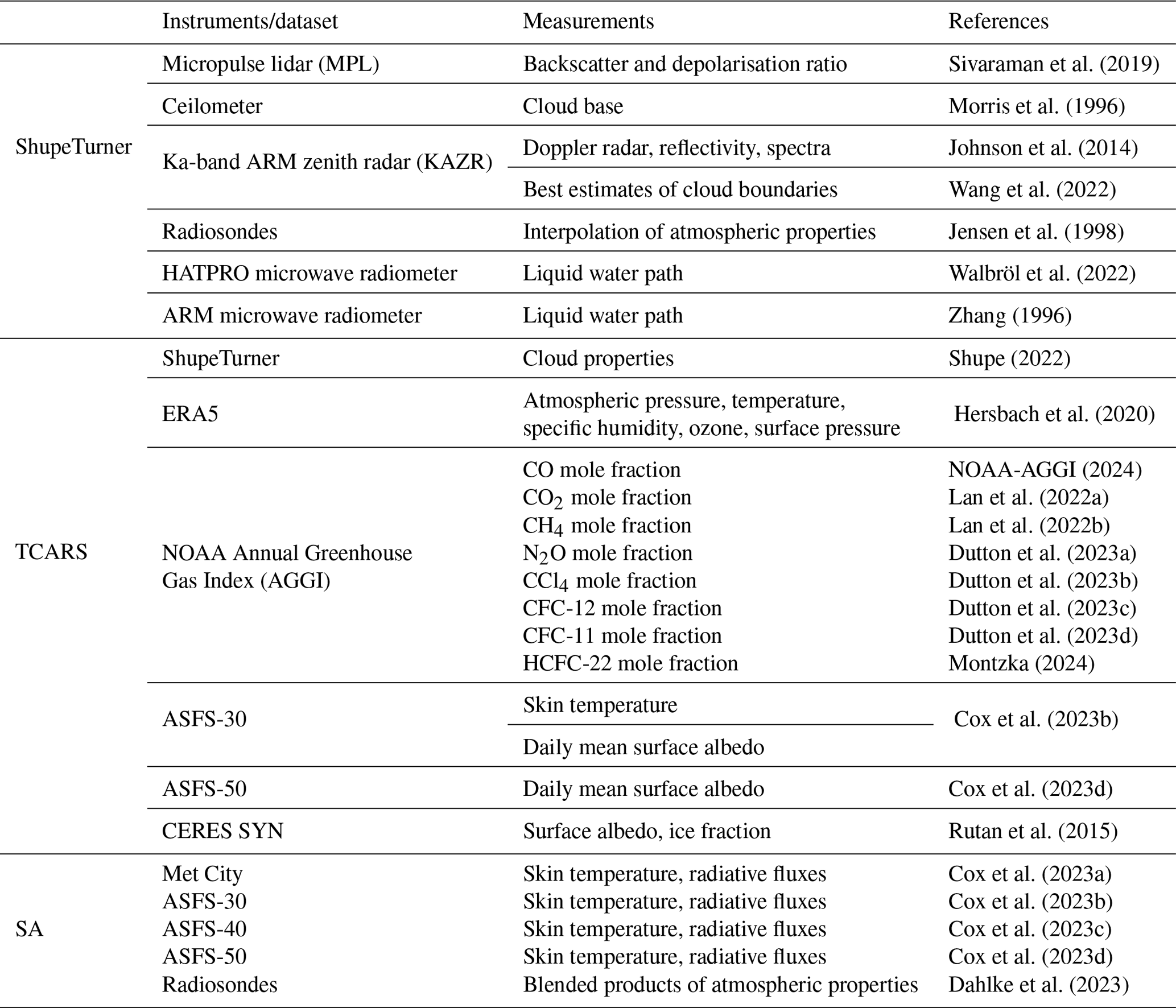
Shupe et al. (2022) and Cox et al. (2023e) provide a detailed overview of the atmospheric remote sensing and in situ meteorological observations carried out on board Polarstern (PS) and at the MOSAiC Surface Observatory (SO), respectively. In this section, we specifically address the observations used in this study as referenced in Table 1.

Sivaraman et al. (2019)Morris et al. (1996)Johnson et al. (2014)Wang et al. (2022)Jensen et al. (1998)Walbröl et al. (2022)Zhang (1996)Shupe (2022)Hersbach et al. (2020)NOAA-AGGI (2024)Lan et al. (2022a)Lan et al. (2022b)Dutton et al. (2023a)Dutton et al. (2023b)Dutton et al. (2023c)Dutton et al. (2023d)Montzka (2024)Cox et al. (2023b)Cox et al. (2023d)Rutan et al. (2015)Cox et al. (2023a)Cox et al. (2023b)Cox et al. (2023c)Cox et al. (2023d)Dahlke et al. (2023)

Table 1 List of data sources for ShupeTurner retrievals as well as for the radiative transfer simulations (TCARS), and for supplementary analysis (SA).

2.1.1 Shipborne instrumentation

On board Polarstern there was a suite of active and passive remote sensing instruments used to observe cloud and aerosol properties during MOSAiC. This instrumentation was installed on Polarstern's foredeck at about 10 m a.s.l. (see Fig. 3 in Shupe et al., 2022). As part of the ARM Mobile Facility (Miller et al., 2016), a 35 GHz Ka-band ARM zenith radar (KAZR) provided information on radar reflectivity, mean Doppler velocity, and spectrum width (Johnson et al., 2014; Wang et al., 2022). A high-spectral-resolution lidar and a micropulse lidar were installed, providing information about the backscatter and depolarisation ratio (Morris et al., 1996; Sivaraman et al., 2019). The atmospheric liquid water path (LWP) was derived from a combination of two microwave radiometers, a two-channel sensor (Zhang, 1996), and a humidity and temperature profiler (HATPRO) (Ebell et al., 2022; Walbröl et al., 2022). In addition, radiosondes were launched every 6 h from Polarstern to provide information about the thermodynamic and kinematic state of the atmosphere (Maturilli et al., 2021).

The combination of instruments and radiosonde observations is used to characterise cloud and aerosol properties during MOSAiC. Section 3.1 summarises the methodology used to derive the macro- and microphysical properties of clouds.

2.1.2 Ice-floe observations

During the MOSAiC expedition, several observations of surface and meteorological properties were measured at different locations of the SO. A 10 m meteorological tower and a radiation station were deployed at Met City. Three mobile atmospheric surface flux stations (ASFSs), named ASFS-30, ASFS-40, and ASFS-50, were deployed in the MOSAiC distributed network. The spatial distance of these observations ranged from hundreds of metres to approximately 20 km relative to the location of Polarstern, as shown in Fig. 3 of Cox et al. (2023e). For this study we use the Met City and ASFS observations of skin temperature and the broadband terrestrial (Terr) and solar (Sol) upwelling and downwelling radiative fluxes. While upwelling fluxes may express local variability, the downwelling fluxes are considered regionally representative (Rabe et al., 2024). For clarity, the paper uses the terms solar and terrestrial radiation to refer to broadband shortwave and longwave radiation, respectively (see Appendix A1).

The temporal coverage of surface radiation observations varied across the MOSAiC period. Observations at Met City were made from mid-October 2019 to mid-May 2020 followed by data collection from the end of June to July 2020, after which the ice floe broke apart at the edge of the ice pack. From the beginning of August to mid-September 2020, Met City observations were made again from a new ice floe farther north. ASFS-30 had the largest temporal coverage and collected data from mid-October 2019 to mid-September 2020, with a few gaps in November 2019, February 2020, May 2020, and the end of August. ASFS-40's observations were continuous from early October 2019 to the end of March 2020, while ASFS-50's observations were made from early October 2019 to mid-September 2020 but with significant data gaps between mid-January and mid-March 2020, May into June 2020, and early August 2020. The narrative is similar for each station; each variable was quality-controlled and some smaller gaps were present for several hours due to quality issues and maintenance (Cox et al., 2023e).

The upwelling and downwelling broadband solar radiative fluxes at Met City were measured by upward-looking and downward-looking Eppley precision spectral pyranometers (PSPs; 0.285–3.0 µm), whereas the terrestrial fluxes were measured with Eppley precision infrared radiometers (PIRs; 3.5–50 µm) at 1 Hz (see Table 1 in Cox et al., 2023e). At ASFS stations, downward- and upward-looking pyranometers were Hukseflux SR30-D1 models and pyrgeometers were IR20-T2 models (Cox et al., 2023e). The skin temperature provided at all four sites was derived using information from both upwelling and downwelling terrestrial observations, assuming a surface emissivity of 0.985 (see Eq. 3 in Cox et al., 2023e). The sensor heights were approximately 2 m above the surface.

2.2 Satellite observations and ancillary data

This study uses the CERES SYN1deg Ed. 4 satellite products with hourly resolution (Gupta et al., 2010; Rose et al., 2013; Rutan et al., 2015; Kato et al., 2018; Minnis et al., 2021), referred to here as CERES SYN. The data include global coverage of solar and terrestrial radiative fluxes at the top of the atmosphere and at the surface with a spatial resolution of 1° latitude by 1° longitude. Fluxes at the top of atmosphere are inferred from CERES radiance observations using empirical angular directional models. Fluxes within the atmosphere and at the surface are calculated using the four-stream Langley Fu–Liou radiative transfer model (Fu and Liou, 1992; Kato et al., 2005), adjusting inputs to ensure consistency with the TOA fluxes. The cloud properties used in these calculations were derived from Moderate Resolution Imaging Spectroradiometer (MODIS) radiances (Minnis et al., 2021). Temporal interpolation is achieved at lower latitudes by means of geostationary satellite observations, while it relies on the improved temporal sampling of polar-orbiting satellites in polar regions. The CERES SYN products also use atmospheric reanalysis data from the Global Modeling and Assimilation Office Goddard Earth Observing System model version 5.4.1 (GEOS-5.4.1) as ancillary input (Rienecker, 2008). Furthermore, surface spectral albedo is based on lookup tables from Jin et al. (2004), and the broadband albedo is based on Terra surface albedo history maps that are consistent with clear-sky TOA albedo estimates from CERES measurements (Rutan et al., 2015).

The CERES SYN radiative fluxes are given considering four different atmospheric scenarios: an all-sky (AS) atmosphere, which takes into account both clouds and aerosols; a cloudless sky (CS) atmosphere, which considers only the presence of aerosols; a pristine (Pr) atmosphere, where there are no clouds or aerosols are present; and finally, an all-sky no-aerosol (NAER) atmosphere, where clouds are present but no aerosols are considered.

Besides the radiative flux datasets, various surface, cloud, and aerosol parameters are included in the CERES SYN dataset. Considered in this study are the cloud base pressure (P_B), cloud top pressure (P_T), cloud top temperature, cloud base temperature, cloud fraction (CF), LWP, ice water path (IWP), liquid droplet effective radius r_E, L, and ice crystal effective radius r_E, I. The latter products are available for the entire atmospheric column and at four different heights (i.e. surface to 700, 700–500, 500–300, and higher than 300 mbar). The CERES SYN products use the aerosol optical depth (AOD) obtained from the Model of Atmospheric Transport and Chemistry (MATCH; Collins et al., 2001) data that assimilate retrievals from MODIS (Rutan et al., 2015).

Several ancillary datasets were used as input parameters for the radiative transfer simulations and overall analysis in this article. We used pressure-level profiles of temperature, pressure, the ozone mass mixing ratio, and specific humidity from the European Centre for Medium-Range Weather Forecasts (ECMWF) Reanalysis v5 (ERA5) (Hersbach et al., 2020) at 1 h resolution and 0.25° spatial latitudinal and longitudinal resolution. Additionally, dry-air mole fractions of carbon dioxide; nitrous oxide; methane; chlorofluorocarbons, specifically CFC-11 and CFC-12; and carbon tetrachloride (CCl₄) from NOAA Global Monitoring Laboratory's Annual Greenhouse Gas Index (AGGI; https://gml.noaa.gov/aggi/aggi.html, last access: 1 March 2024) were used. To characterise the atmosphere, we used radiosonde data that were processed to remove the influence of Polarstern and blended with Met City data to better represent near-surface meteorology, as the radiosondes were launched from the deck at approximately 20 m height (Dahlke et al., 2023).

3 Methodology

3.1 ShupeTurner cloud retrievals for MOSAiC

The ShupeTurner cloud retrievals provide time-resolved vertical profiles of the macro- and microphysical properties of clouds based on active and passive remote sensing observations. The retrievals were first introduced in Shupe et al. (2015) (hereafter ST2015) and applied to observations at the NSA site (71.323° N, 156.615° W) for the 2-year period from March 2004 to February 2006. ST2015 describe the algorithm, including both its assumptions and its uncertainties. Moreover, a comparison with the ARM MICROBASE cloud product (Dunn et al., 2011), as well as a closure analysis of solar and terrestrial downward fluxes, has been presented. The results in ST2015 indicated that ShupeTurner performed better than the ARM MICROBASE cloud retrievals.

As applied to MOSAiC, the ShupeTurner retrievals utilise cloud radar, depolarisation lidar, microwave radiometer, ceilometer, and radiosonde observations collected on board Polarstern as inputs (see Table 1). Reflectivities from the KAZR were adjusted above 3 km to statistically match the observations below 3 km due to a known calibration offset between two different radar operational modes. The low-level measurements have been determined to have the best calibration during MOSAiC. Short gaps in the KAZR data were filled using a collocated W-band cloud radar. The calibration of this radar was adjusted to align with temporally adjacent KAZR measurements. The LWP data were taken from either of the two microwave radiometers to ensure maximum coverage.

Several improvements beyond ST2015 were made in the cloud-phase classification (Shupe, 2007). A novel set of thresholds were developed from the cloud-free background on the micropulse signal-to-noise ratio lidar and total backscatter measurements using the MOSAiC data. The cloud phase was also corrected to account for lidar attenuation in the presence of liquid-containing cloud layers. For such cases, if the cloud radar observes a cloud top that is within 750 m, then the same cloud type is considered from the attenuation height up to the cloud top. In contrast to the retrievals for NSA site, the default liquid droplet effective radius was changed from 8 to 9 µm, which is based on aircraft measurements from the region (Shupe et al., 2005). The effective radius is also calculated for liquid droplets (r_E, L) and ice crystals (r_E, I), along with the vertical integral of LWP and IWP.

ShupeTurner products provide information on cloud type phase as well as the content of liquid (LWC) and ice water (IWC). The dataset has a 1 min time resolution and covers a vertical range from 160 m up to 18 km by 596 equidistant height layers, each with a thickness of 30 m.

3.2 Single-column radiative transfer configuration

The radiative transfer simulations are carried out with the TROPOS Cloud and Aerosol Radiative effect Simulator (hereafter TCARS), a Python-based framework for 1D radiative transfer simulations with interfaces with a number of radiative transfer models. Parts of this framework have already been applied and described in previous studies (Barlakas et al., 2020; Witthuhn et al., 2021; Barrientos-Velasco et al., 2022; Griesche et al., 2024a, b). TCARS can use various sources for input data such as atmospheric profiles of trace gases, temperature, humidity, cloud properties, and surface parameters. The present study employs the widely used Rapid Radiative Transfer Model (RRTM) for general circulation model (GCM) applications as a solver (RRTMG; Mlawer et al., 1997; Barker et al., 2003; Clough et al., 2005). The Python interface pyRRTMG, version 0.9.1 (Deneke, 2024), is used by TCARS. The overall workflow of the TCARS framework is shown in Fig. A1, detailing the input parameters and the output variables derived from the radiative transfer simulations.

The input parameters for the radiative transfer simulation configuration are listed in Table 1. For the atmospheric profiles of temperature, pressure, humidity, and ozone, we use hourly pressure-level profiles from ERA5, which assimilate information from the Vaisala Radiosonde RS41, which was launched every 6 h during MOSAiC (Hersbach et al., 2020). This dataset was selected due to its consistent temporal and spatial coverage and well-resolved atmospheric data covering up to 20 km as well as it showing good similarities with radiosonde observations (Fig. B1). For trace gases, we used the uniformly distributed values of CO₂, CH₄, N₂O, CCl₄, CFC-12, HCFC-22, and CFC-11 from the Annual Greenhouse Gas Index (AGGI).

The atmospheric profiles of cloud properties are based on ShupeTurner retrievals. The information added to the model is the LWC, IWC, liquid droplet effective radius (r_E, L), and ice crystal effective radius (r_E, I). The RRTMG parameterisations selected for ice and liquid cloud optical properties are based on the radiative transfer model Streamer (Key, 1996) and on Hu and Stamnes (1993), respectively.

Several experiments were conducted based on different surface albedo datasets (see Figs. B3, A1). First, the surface albedo from the CERES SYN product was utilised as an input parameter to calculate the radiative fluxes, denoted TCARSe1. This dataset is interpolated in both space and time to match the position of Polarstern at a 1 min resolution throughout the MOSAiC cruise. We chose to use this dataset as an input parameter since one of our objectives is to quantify flux differences related to cloud properties rather than surface differences. The comparison of ice-floe-measured and surface albedo derived from CERES SYN is discussed in Huang et al. (2022).

The second and third sources of surface albedo come from the observations at the ASFS-30 and ASFS-50 stations (see Fig. B3). The radiative flux calculations derived from these two sources are referred to as TCARSe2 and TCARSe3, respectively. This observed surface albedo was derived by calculating the daily mean ratio between the broadband upwelling and downwelling solar flux. We opted for a daily average to exclude small-scale temporal variability observed at these stations. Note that the rest of the input parameters for TCARSe2 and TCARSe3 remain the same as for TCARSe1.

The objectives of each experiment were to verify the consistency of radiative flux calculations between TCARS and CERES SYN without adding variables (i.e. TCARSe1), to validate ShupeTurner retrievals and quantify the radiation budget and cloud radiative effect (i.e. TCARSe2), and to confirm TCARSe2 results while analysing spatial variability (i.e. TCARSe3).

The surface emissivity is set to a constant value based on the fraction of sea ice in the vicinity of Polarstern, which is also obtained from CERES SYN product. When the sea ice fraction reaches or exceeds 50 %, a constant surface emissivity of 0.9999 is used. If the sea ice fraction is below this threshold, a constant of 0.9907 is used instead. These constant values are based on Wilber et al. (1999). It is worth mentioning that this assumption is not the same as the one assumed for deriving the skin temperature from surface measurements (see Eq. 3 in Cox et al., 2023e). However, we expect that this difference does not exceed more than 1 W m⁻² of the upwelling terrestrial flux (Terr-U) at the surface during cloudless conditions (see Table A2 in Barrientos-Velasco et al., 2022).

Skin temperature is obtained from the derived product by Cox et al. (2023b) at station ASFS-30 due to its extensive temporal coverage. When these data are unavailable, skin temperature from Met City is utilised (Cox et al., 2023a). In instances when no skin temperature data are available but the ShupeTurner product is available, skin temperature from CERES SYN is used instead for completeness. These latter cases were rare but occurred more frequently in August 2020 (i.e. 2 to 8 August 2020).

Several approaches for specifying skin temperature were tested, including using only ERA5 or only CERES SYN. We chose to use derived skin temperature from ice-floe observations at MOSAiC to quantify the flux differences between the CERES SYN product and observations, providing a more realistic calculation of Terr-U. Another version of the simulations using skin temperature from ERA5 is excluded in this article since this data source led to an overestimation of skin temperature, especially during the polar night, when the largest bias was found during cloudless conditions (Herrmannsdörfer et al., 2023).

All input parameters are linearly interpolated to a predefined standard grid consisting of 632 atmospheric levels, which range from 40 to 20 km in altitude. This grid aligns with the CERES SYN TOA height and has a temporal resolution of 1 min. The first 600 levels of the atmosphere were divided into equidistant layers of 30 m each, and from 18.01 to 20 km, each layer was divided into 63.2 m.

A total of 327, 126, and 83 daily NetCDF files were generated for TCARSe1, TCARSe2, and TCARSe3, respectively. The temporal coverage is illustrated in Fig. A2. For convenience, the simulations have been compiled into monthly files, which are available in Barrientos-Velasco (2024). Each file includes simulated profiles of both cloudy and cloudless broadband upwelling and downwelling solar and terrestrial fluxes, heating rates, and direct downwelling solar flux (see Fig. A1).

This study follows the definition by Rossow and Zhang (1995) and Mace et al. (2006) of the cloud radiative effect (CRE) as the difference in radiation between a cloudy and cloud-free atmosphere at the surface and the TOA. In this article, we discuss two calculation methods: one based on the difference between simulated all-sky conditions minus simulated cloudless conditions and another term named “hybrid”, which subtracts the cloudless simulation from the observed radiative flux. This difference is measured in units of W m⁻². The total CRE is calculated by adding the Terr CRE and Sol CRE components, which are calculated using Eq. (1). In this equation, x represents either terrestrial or solar radiation and is calculated at both the surface and the TOA. The atmospheric CRE is defined as the difference between the TOA and the surface. This terminology and methodology are based on previous research by Barrientos-Velasco et al. (2022). A positive value indicates warming, while a negative value indicates cooling due to the presence of clouds.

$$\begin{array}{}\text{(1)}& {\text{CRE}}_x={\left(F_x^{\downarrow }-F_x^{\uparrow }\right)}_{\mathrm{All}\text{-}\mathrm{sky}}-{\left(F_x^{\downarrow }-F_x^{\uparrow }\right)}_{\mathrm{Cloudless}}\end{array}$$

4 Results and discussions

4.1 General overview of atmospheric and surface conditions

RV Polarstern drifted with the Arctic sea ice from the Laptev Sea to the Fram Strait through the central Arctic region from October 2019 to September 2020. We divided the time series into four periods: two during the polar night (from 15 October to 31 December 2019 and from 1 January to 13 March 2020) and two during the polar day (from 14 to 31 May 2020 and from 1 June to 20 September 2020) to characterise seasonal differences (Fig. 1). Additionally, we consider the entire MOSAiC period from 15 October 2019 to 20 September 2020.

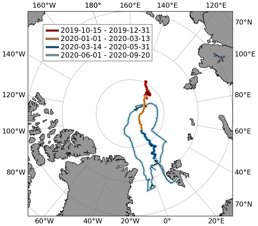
Figure 1 The cruise track of the research vessel Polarstern during the MOSAiC expedition is shown on an Arctic polar stereographic map. The solid red and orange lines show the track during the polar night, and the solid blue and light-blue lines denote the track during the polar day. Each colour represents the period shown in the upper box (date format: year-month-day), discussed in Sect. 4.2.

The second half of October 2019 featured average near-surface meteorological conditions, with 2 m air temperatures dropping from about 263 to 255 K (Rinke et al., 2021). This period saw a high frequency of single-layer clouds (see Fig. 2a) and low-level jets (López-García et al., 2022), possibly contributing to turbulence in the atmosphere and a weakly stable regime (Jozef et al., 2023). Storms began to occur at the MOSAiC location in November, specifically from 16 to 20 November, bringing high winds and moist air from the North Atlantic and leading to the formation of leads and periodic power outages that disrupted measurements (Nicolaus et al., 2022; Cox et al., 2023e). This lead formation coincided with a decrease in sea ice thickness (Krumpen et al., 2021), and integrated water vapour increased significantly from 2 to 8 kg m⁻² (Heinemann et al., 2023), reaching record-breaking levels relative to climatology (Rinke et al., 2021).

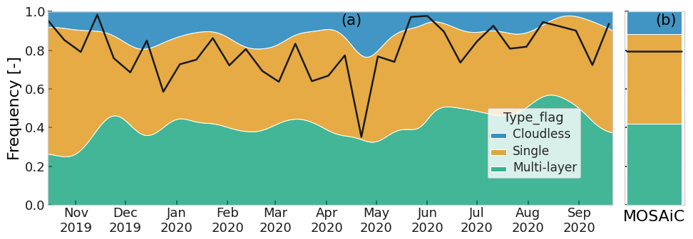
Figure 2 Time series showing the occurrence and composition of clouds during MOSAiC. Panel (a) shows the occurrence frequency of cloudless conditions (blue), single-layer clouds (orange), and multi-layer clouds (green), while the black line shows the cloud fraction from CERES SYN. The black line in panel (a) shows the 10 d averaged normalised cloud area fraction from CERES SYN, and mean values are shown in the solid black line in panel (b).

The coldest atmospheric conditions were observed from December to mid-March (Herrmannsdörfer et al., 2023). The 2 m air temperature decreased to as low as 231 K (Fig. B2). However, there were two exceptions to this pattern. In early December (3–5 December) and in February (18–22 February), warm air-mass intrusions (WAIs) originating from Siberia reached MOSAiC, causing a temporary increase in temperature (Herrmannsdörfer et al., 2023; Rinke et al., 2021). A marine cold-air outbreak (MCAO) was identified in March, with the centre over the Fram Strait region and linked to northerly winds (Rinke et al., 2021; Murray-Watson et al., 2023). From January to March 2020, a record-breaking positive phase of the Arctic Oscillation index was observed, indicating that the low-pressure anomaly in the Arctic was surrounded by a ring of high pressure at mid-latitudes that potentially facilitated the transport of mid-latitude air masses (Lawrence et al., 2020; Rinke et al., 2021; Boyer et al., 2023).

April 2020 was characterised by two WAIs that led to an anomalous increase in near-surface air temperature from 242.4 to 270.0 K from 14 to 21 April (Shupe et al., 2022). The analysis of Kirbus et al. (2023) suggested that this WAI was associated with a Siberian and Atlantic air mass that led to a strong positive effect on the surface energy budget dominated by turbulent heat fluxes over the ocean and strong radiative influence over sea ice. The increase in temperature during this event was associated with the increase in the concentration of water vapour with values that exceeded 10 kg m⁻² (Kirbus et al., 2023). This unprecedented increase in temperature led to several changes in conditions in the atmosphere (Dada et al., 2022; Svensson et al., 2023) and at the surface (Krumpen et al., 2021; Rückert et al., 2023). This period was also used as a first example of the improvement in how nudging a large-scale circulation model to observations improved and accelerated the model evaluation (Pithan et al., 2023).

May was characterised by anomalously warm temperatures that were more prominent during the second half of the month (Rinke et al., 2021). From mid-May to June, Polarstern left the MOSAiC SO for an exchange of personnel at the fjord of Svalbard (Shupe and Rex, 2022). The months of July and August were considered the warmest recorded for the 1979–2020 period. The atmospheric conditions during this period were moister than the climatological values, with the total column water vapour reaching up to 30 kg m⁻² (Rinke et al., 2021). In July 2020, a significant decrease in surface albedo was observed, led by an increase in the melt-pond fraction by 20 % (Webster et al., 2022), especially between 11 and 13 July, when melt-pond drainage was observed (Webster et al., 2022; Light et al., 2022).

Finally, in September 2020, the near-surface temperatures started to decrease to temperatures below 273.15 K, allowing ice-floe ponds to freeze up (Webster et al., 2022; Light et al., 2022). Two WAIs were observed in the middle of September that were associated with an increase in humidity, temperature, and heat transport from lower latitudes (Rinke et al., 2021).

Complementing the previous description, Fig. 3 illustrates the microphysical cloud properties based on CERES SYN and ShupeTurner. The monthly variations in the LWP and IWP are depicted in box plots, and the annual variations in r_E, L and r_E, I are shown at four different heights corresponding to those described in the CERES SYN products (see Sect. 2.2). For CERES SYN and ShupeTurner, the values of LWP increase during the polar day, which is expected as atmospheric temperature increases. The IWC decreases during summer based on the ShupeTurner dataset, but CERES SYN does not follow the same tendency. It is important to note that the CERES SYN statistics are influenced by periods with optically thick clouds, and there are times when the presence of clouds is either missed or underestimated (see Fig. 2). r_E, L shows variation with height according to the CERES SYN data, while the ShupeTurner dataset maintains a constant value of 9 µm. Conversely, r_E, I is greater in the ShupeTurner data compared to the CERES SYN data, showing an overall decrease with height.

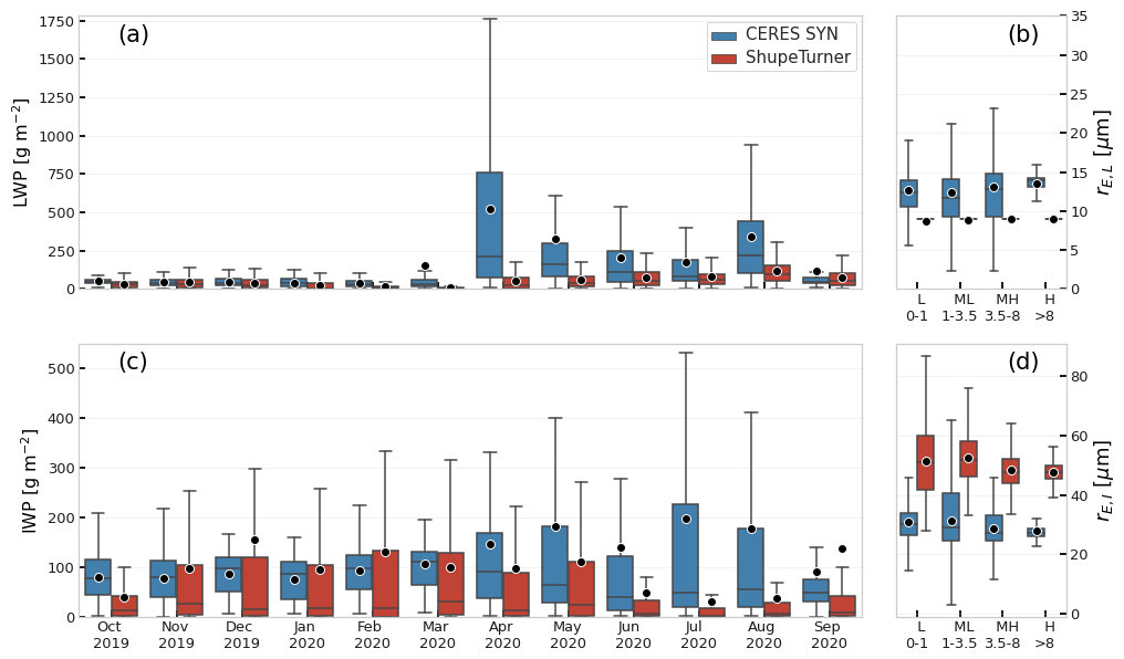
Figure 3 Time series of cloud water paths based on the ShupeTurner and CERES SYN retrievals. Panels (a) and (c) show box plots of monthly statistics of the liquid water path (LWP) and ice water path (IWP), respectively for the CERES SYN (blue) and ShupeTurner (red) datasets. Panels (b) and (d) show statistics of the vertical profiles of the liquid droplet (r_E, L) and ice crystals (r_E, I) effective radius for low-level (L; 0–1 km), mid- to low-level (ML; 1–3.5 km), mid- to high-level (MH; 3.5–8 km), and high-level clouds (H; > 8 km) for the entire MOSAiC expedition. Boxes in panels (a)–(d) extend from the 25th to 75th percentile, the median is represented by a line, and the black dots depict the mean.

4.2 Consistency between cloudless fluxes

In this section, we will focus on the TCARSe1 cloudless simulations (see Sect. 3.2, Fig. A2). The TCARSe1 simulations and CERES SYN product rely on different data sources for atmospheric and surface conditions, such as skin temperature and atmospheric profiles of humidity and temperature. They also use different radiative transfer models. Therefore, prior to conducting the all-sky radiative closure assessment for the MOSAiC period, it is necessary to understand the differences between both fluxes under cloudless conditions. This understanding will be important for the subsequent calculations of the cloud radiative effect.

This analysis focuses on all available TCARSe1 simulations from 15 October 2019 to 20 September 2020 and CERES SYN products collocated to the location of Polarstern. The analysis includes a comparison of downwelling and upwelling terrestrial and solar fluxes at the surface and an upwelling comparison at the TOA. The dataset was divided into two periods during the polar night and two during the polar day as illustrated in Fig. 1.

The comparison of cloudless downwelling terrestrial flux (Terr-D) at the surface reveals high correlations (over 0.9) between TCARSe1 and CERES SYN, with biases not exceeding 9.6 W m⁻² (not shown). Discrepancies occurred from 16–19 October and 11–22 November, when TCARSe1 fluxes exceeded CERES SYN by average differences of 25.2 and 32.3 W m⁻², respectively. The November discrepancies coincided with high cloud occurrence during the WAI period. However, a cloudless period on 13 November showed good agreement between TCARSe1 simulations and ASFS-40 station observations, with mean (maximum) flux differences of 1.8 W m⁻² (5.3 W m⁻²).

The comparison of cloudless Terr-U at the surface showed consistent agreement between both datasets, with biases under 5.9 W m⁻² and correlations over 0.87. However, the skin temperature comparison in Fig. B2 reveals a discrepancy in September 2020, when CERES SYN values were lower than MOSAiC SO observations. The largest difference was observed from 14–20 September 2020, with a mean flux difference of 21.6 W m⁻² and a maximum 27.5 W m⁻², coinciding with two storms that caused rain on snow, as noted in prior studies (Rinke et al., 2021; Shupe et al., 2022).

The cloudless comparison of downwelling solar flux (Sol-D) is shown in Fig. C1a, b, e, and f. The correlation coefficient is nearly 1.0, and the distributions reveal an unimodal pattern centred near zero for both cloudless and pristine conditions (green). The mean flux differences from 14 March to 31 May 2020 are 2.9 W m⁻² for cloudless and −3.1 W m⁻² for pristine conditions.

From 1 June to 20 September 2020, TCARSe1 simulations and CERES SYN pristine products show good agreement. The comparison between CERES SYN cloudless and pristine products suggests that the presence of aerosols reduces Sol-D by 6.0 W m⁻² during the first polar-day period and 15.3 W m⁻² during the second polar-day period.

All versions of TCARS simulations do not account for the presence of aerosols in the atmosphere, given that the main focus was on the influence of clouds on the radiation budget; nonetheless, these differences due to the presence of aerosols are considered in the analysis presented in the following sections.

The mean upwelling solar flux (Sol-U) difference between TCARSe1 simulated fluxes and the CERES SYN product at the surface is 2.4 W m⁻² for the first polar-day period (Fig. C1c) and 7.2 W m⁻² for the second polar-day period (Fig. C1d). The comparison between TCARSe1 and CERES SYN pristine products shows biases of −2.6 and −2.0 W m⁻² for the respective polar-day periods. Differences arise since the presence of aerosols reduces the amount of solar radiation reaching the surface, thereby decreasing its availability to be reflected. Consequently, the similarity in kernel density estimate (KDE) distributions of Sol-D and Sol-U reflects the dependence of both components on the radiative transfer calculations.

At the TOA, the cloudless Terr-U and Sol-U exhibit good agreement between TCARSe1 simulations and the CERES SYN product. All correlation coefficients are higher than 0.89, and the distributions are centred around zero. The mean flux differences are below ±4.5 W m⁻² within the instrumental uncertainty and consistent between both datasets (not shown).

In general, the cloudless comparison between TCARSe1 simulations and the CERES SYN product suggests a reliable comparison. Nevertheless, it is important to consider the periods during which the disagreement is more significant due to an underestimation of temperature and humidity from CERES SYN leading to an underestimation of Terr-D and the omitted direct influence of aerosols under cloudless conditions reducing Sol-D for TCARS simulations.

4.3 Radiative closure assessment

The three TCARS sets of simulations (i.e. TCARSe1, TCARSe2, and TCARSe3) and CERES SYN product are evaluated within the context of a radiative closure study that is defined as acceptable if the biases are within the assessed uncertainty in the measurements. To be consistent with previous studies (i.e. Dong et al., 2016; Ebell et al., 2020; Barrientos-Velasco et al., 2022), we consider acceptable biases no larger than ±10.0 W m⁻² for Terr-D and ±20.0 W m⁻² for Sol-D as these values are considered to be the maximum uncertainty in polar regions (Lanconelli et al., 2011). The global annual mean net surface flux uncertainties for the CERES SYN product are within ±12.0 W m⁻²; however, larger uncertainties are expected in the polar regions, especially in the upward solar flux (Kato et al., 2012).

Barrientos-Velasco et al. (2022) examined how uncertainties in various input parameters, such as atmospheric temperature, water vapour, skin temperature, ozone, and surface albedo, propagate through radiative transfer simulations under clear-sky conditions. The findings indicated that the propagated uncertainty in the radiative fluxes was ±2.6 W m⁻² for Terr-D and ±3.7 W m⁻² for Sol-D. Potential uncertainties in the cloud product arise from input measurements, the categorical classification of cloud types, and the retrievals applied, and these interact in complex ways with the variable environmental uncertainties associated with spatial variability and scale mismatches for different observations and parameters. While it is nearly impossible to disentangle or quantify the individual impacts of these uncertainties, the radiative closure employed here is one means for assessing the overall uncertainty in all components collectively.

The following radiative closure assessment focuses on comparing the simulated terrestrial and solar fluxes with the observed fluxes at the surface and TOA. At the surface, the radiative closure is considered only for downwelling fluxes, while at the TOA, it is considered for upwelling fluxes. The counterparts are not evaluated as they are less dependent on clouds and the simulations use them as inputs, such as skin temperature (e.g. TCARSe1, TCARSe2, TCARSe3) and surface albedo (e.g. TCARSe2, TCARSe3). Moreover, we aim to be consistent with the methodology presented in ST2015.

Additionally, we categorise the comparison by atmospheric conditions into four main categories: all-sky, cloudy, cloudless, and broken-cloud conditions, as classified by ShupeTurner. Broken-cloud conditions were derived from the cloudless screening and were identified in instances where the standard deviation among downwelling flux observations from stations exceeded 10.0 W m⁻² during periods when more than one downwelling pyranometer or pyrgeometer was available. Including the category of broken-cloud conditions in the analysis aims to remove any cloud contamination in the cloudless analysis. Achieving a good representation of cloudless conditions is the first step in validating the radiative transfer simulations and separating cases that are outside the scientific objectives of the current study. Our analysis does not further investigate the similarities or discrepancies of the cloud phase between ShupeTurner retrievals and the CERES SYN product.

The comparison includes all available high-quality ice-floe observations from ASFS stations and at Met City while excluding periods with rain. Rainy conditions introduce interference, by either disrupting the microwave radiometer measurements (Cadeddu et al., 2017) or obstructing the view of upward-looking pyranometers and pyrgeometers.

This section is divided into two parts. The first subsection presents a comparison between simulated and observed downwelling terrestrial and solar fluxes at the surface, and the second section compares the upwelling terrestrial and solar fluxes at the TOA.

For clarity, the analysis with TCARS simulations will refer to experiment TCARSe2 for the solar and terrestrial fluxes. Note that the analysis of the terrestrial flux is extended to the data availability of TCARSe1 (Fig. A2), as the parameter that was altered in the input (i.e. surface albedo) does not influence the calculations of terrestrial fluxes.

4.3.1 Analysis at the surface

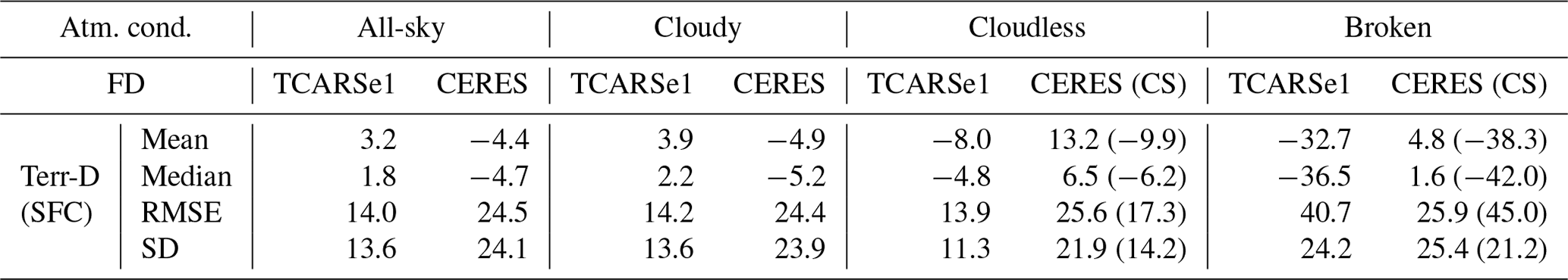
The comparison between simulated Terr-D fluxes and observations at ASFS-30 shows very good agreement for TCARSe2 results, with median hourly differences below ±5 W m⁻², for all-sky, cloudy, and cloudless atmospheric conditions (Fig. 4a, b, c; Table 2). The comparison with CERES SYN also indicates very good agreement for these conditions. However, larger differences are found for the defined cloudless atmosphere, with a median difference of 6.5 W m⁻² (Table 2). Using CERES SYN cloudless products instead of all-sky products suggests that while cloudless conditions are identified at Polarstern, other clouds were present within the spatial resolution of CERES SYN, reducing the biases from 13.2 to −9.9 W m⁻² (see values in parentheses in Table 2). For both datasets, TCARSe2 and CERES SYN, the simulated Terr-D for cloudless conditions shows negative biases that are compensated for by the presence of clouds. Due to the limitations of the 1D experimental radiative transfer setup from TCARS and CERES SYN, larger biases can be expected under broken-cloud conditions, which occurred about 0.6 % of the time (Fig. 4d, l).

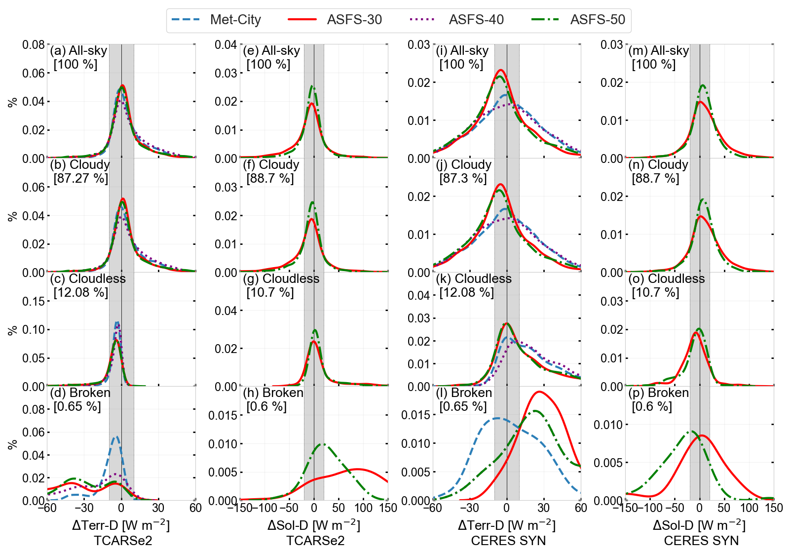
Figure 4 Kernel density estimate (KDE) of the distribution of differences between simulated and observed radiative fluxes at the surface. The first two columns show the KDE for the TCARS simulations, while the last two columns show the KDE for CERES SYN collocated to the positions of Met City, ASFS-30, ASFS-40, and ASFS-50.

Table 2 The hourly downwelling terrestrial flux difference (FD) at the surface (SFC) for the entire MOSAiC period under different atmospheric conditions in W m⁻². Results are based on TCARS simulations, the CERES SYN product (CERES), and observations at ASFS-30. An additional comparison for CERES SYN cloudless (CS) products is given for cloudless and broken-cloud conditions.

The overall hourly TCARSe2 Terr-D comparison among all stations indicated good agreement, suggesting that, in general, Terr-D is similar despite the distances separating each station (Fig. D1a). This finding aligns with Rabe et al. (2024), who reported that in transient conditions, the temporal variability in Terr-D was larger than the spatial variability. The spatial comparison of the collocated CERES SYN product with each station suggests that the mean flux difference is relatively dependent on the location of the observations. According to CERES SYN, the atmospheric conditions might have varied to some extent relative to the location of Polarstern (Fig. D2a).

The KDE distribution of the Sol-D difference between simulations and observations is illustrated in the second and fourth column in Fig. 4 for TCARSe2 and CERES SYN, respectively, and a summary of the biases including all the simulations is shown in Table 3. The lowest biases found are for TCARSe2 with mean and median flux differences below ±4.1 W m⁻² for all-sky and cloudy conditions. The largest biases are found for cloudless conditions for all the simulations, but they are within the uncertainty threshold of ±20 W m⁻². In general, the radiative closure can be confirmed for TCARS simulations and CERES SYN.

Table 3 Hourly downwelling solar flux (Sol-D) difference (FD) at the surface (SFC) for the entire MOSAiC period under different atmospheric conditions in W m⁻². Results are shown for CERES SYN (CERES) products, TCARS simulations using different surface albedo levels based on CERES SYN surface albedo (TCARSe1), and the daily mean from observations at ASFS-30 (TCARSe2) and at ASFS-50 (TCARSe3). An additional comparison for CERES SYN cloudless (CS) products is given for cloudless and broken-cloud conditions.

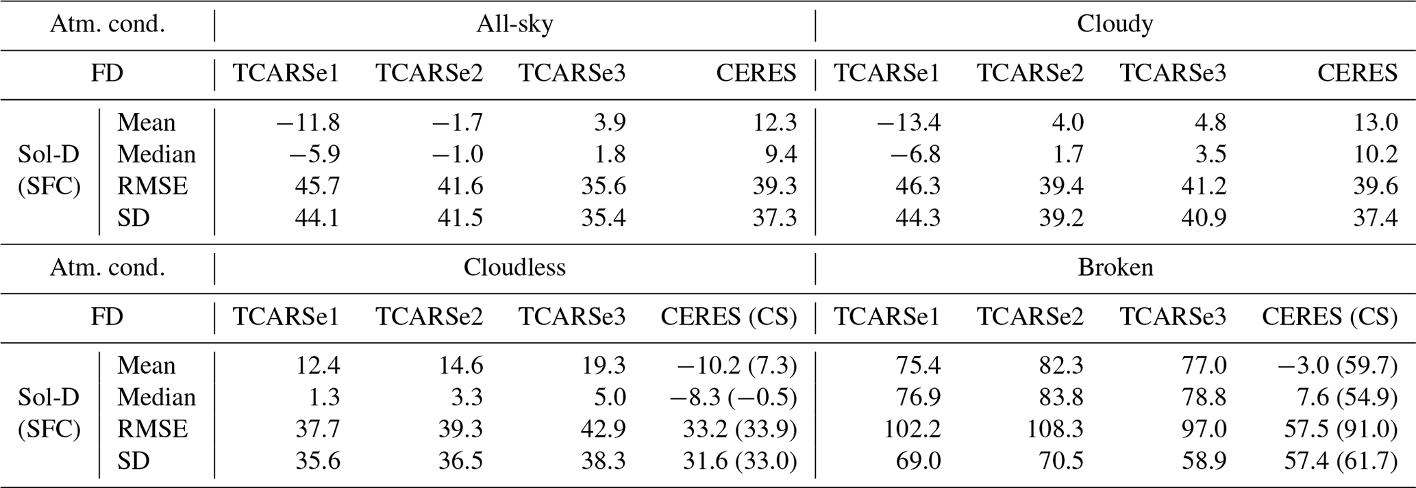
The Sol-D comparison between TCARSe1 and TCARSe2 directly shows the effect that surface albedo has on radiative transfer calculations. Both TCARSe1 and TCARSe2 use the same cloud properties, but the change in surface albedo causes a mean flux difference of about 10 W m⁻² in Sol-D (Table 3). Note that the viewing differences between ground-based and satellite sensors are another factor leading to the flux differences as the ground-based observations cover an area of a few metres. In contrast, the satellite perspective has a viewing area with multiple ice floes and an open ocean. Since the ground measurements are used for the comparisons here, it is not surprising that the TCARSe2 and TCARSe3 datasets would show closer agreement.

In the study of Huang et al. (2022), several perturbation experiments were conducted varying the surface albedo and the cloud fraction. This study found that by increasing the surface albedo and the cloud fraction, the biases in the solar and terrestrial fluxes were reduced, suggesting that the surface albedo and atmospheric opacity within the CERES SYN product are underestimated. Our results corroborate their findings, but what we find counter-intuitive is that in general the values of LWP and IWP are larger for CERES SYN than for ShupeTurner (Fig. 3). The latter might also be related to the size of cloud liquid droplets. The size of r_E, L is comparatively large for CERES SYN compared to ShupeTurner, resulting in a smaller optical depth as less sunlight is reflected. It should also be considered that the cloud parameterisations or setup used when calculating the radiative fluxes varies significantly between the radiative transfer solver RRTMG and the four-stream Langley Fu–Liou radiative transfer model. While it is outside the scope of this study to investigate model differences, it is reported that the differences between both models are within the uncertainties set by this study of ±10.0 W m⁻² for Terr-D and ±20.0 W m⁻² for Sol-D (Gu, 2019).

The analysis of Sol-D utilises observations from ASFS-30 and ASFS-50 (Figs. D1b, D2b). No observations were available from ASFS-40 during the polar day, and measurements from Met City are excluded due to a systematic error that caused lower Sol-D values for optically thin atmospheres (e.g. cloudless skies or thin ice clouds). The mean Sol-D difference between Met City and ASFS-50 observations varied by approximately 18 W m⁻² under these conditions. The underestimation of Sol-D observed at Met City may be attributable to the instrumental limitations of the pyranometer at Met City (i.e. Eppley PSP), which is sensitive to incident viewing angles. More details and implications of this sensitivity for surface-based radiometric reference datasets over the global oceans are discussed in Riihimaki et al. (2024).

The ShupeTurner cloud retrievals were evaluated previously in ST2015 considering 2-year atmospheric observations at the NSA site. The radiative closure assessment in ST2015 focused on the downwelling fluxes at the surface and upwelling fluxes at the TOA. The results discussed here are similar to the results reported in ST2015. The largest median flux difference is for cloudless Sol-D with median flux values of −15.6 W m⁻², whereas in this study the median flux difference is 3.3 W m⁻² (Table 3). The Sol-D difference in ST2015 might be due to broken-cloud conditions that had an unquantified impact on their analysis. Note that the results presented in ST2015 were 10 min averages, whereas here the results are hourly averages.

The analysis of ST2015 further investigated the radiative closure assessment by sub-classifying the cloud phase of single-layer clouds into liquid, ice, and mixed phase. Conducting a similar analysis, TCARSe2 results indicate very good agreement for Terr-D at the surface for the three thermodynamic conditions (i.e. liquid, ice, and mixed-phase clouds) with hourly median flux differences below ±4.1 W m⁻² (Table A1).

The results for the Sol-D comparison considering the three versions of TCARS simulations are shown in Table A2. At the SFC, the best agreements are found for TCARSe2 and TCARSe3, with median flux differences below ±6.6 W m⁻². When looking at the mean biases, liquid clouds show the best agreement. For ice clouds, there is a positive bias for TCARS of about 20 W m⁻², suggesting an underestimation in cloud opacity, and in mixed-phase clouds, there is a negative bias of 8.4 W m⁻². The effect of different surface albedo levels between TCARSe1 and TCARSe2 in single-layer liquid and mixed-phase clouds leads to a mean flux difference of about 12.4 W m⁻², suggesting that with a lower surface albedo, less solar radiation is available for multiple reflections between clouds and the surface. The same effect is observed for ice clouds, but to a lesser extent (4.1 W m⁻²), as they scatter Sol-D more effectively.

It is important to note that these results are subject to sample availability and hourly averaging. Increasing the time resolution of the analysis could highlight the influence of advection on observations, thereby enhancing the spatiotemporal variability in the radiative fluxes (Barrientos Velasco et al., 2020; Rabe et al., 2024). Additional analysis on how surface albedo affects the derivation of atmospheric fluxes is recommended for future studies. Improving or refining this parameter is beyond the scope of the current analysis.

4.3.2 Analysis at the top of the atmosphere

The comparison of the upwelling radiative fluxes at the TOA are illustrated in Figs. 5 and D3 and are reported in Tables 4 and 5. The comparison shows the difference between TCARS simulations and the collocated CERES SYN product at the locations of all the stations at the MOSAiC SO. Besides evaluating the TCARS simulations at the TOA, we aim to analyse how the spatial coverage influenced the flux differences.

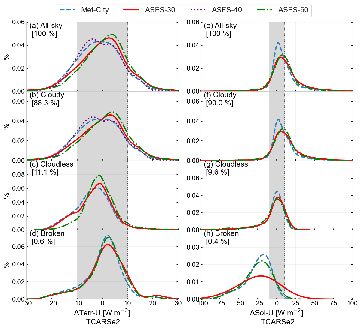
Figure 5 The same as Fig. 4 but comparing the KDE of the difference between TCARS and CERES SYN fluxes at the TOA.

Table 4 Hourly radiative flux difference (FD) at the top of the atmosphere (TOA) for the entire MOSAiC period under different atmospheric conditions. Results are based on TCARS simulations and are in W m⁻².

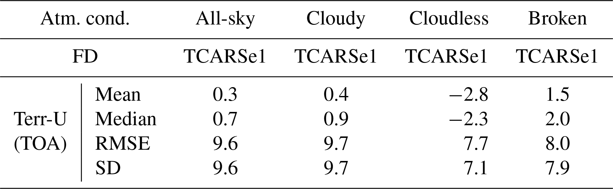
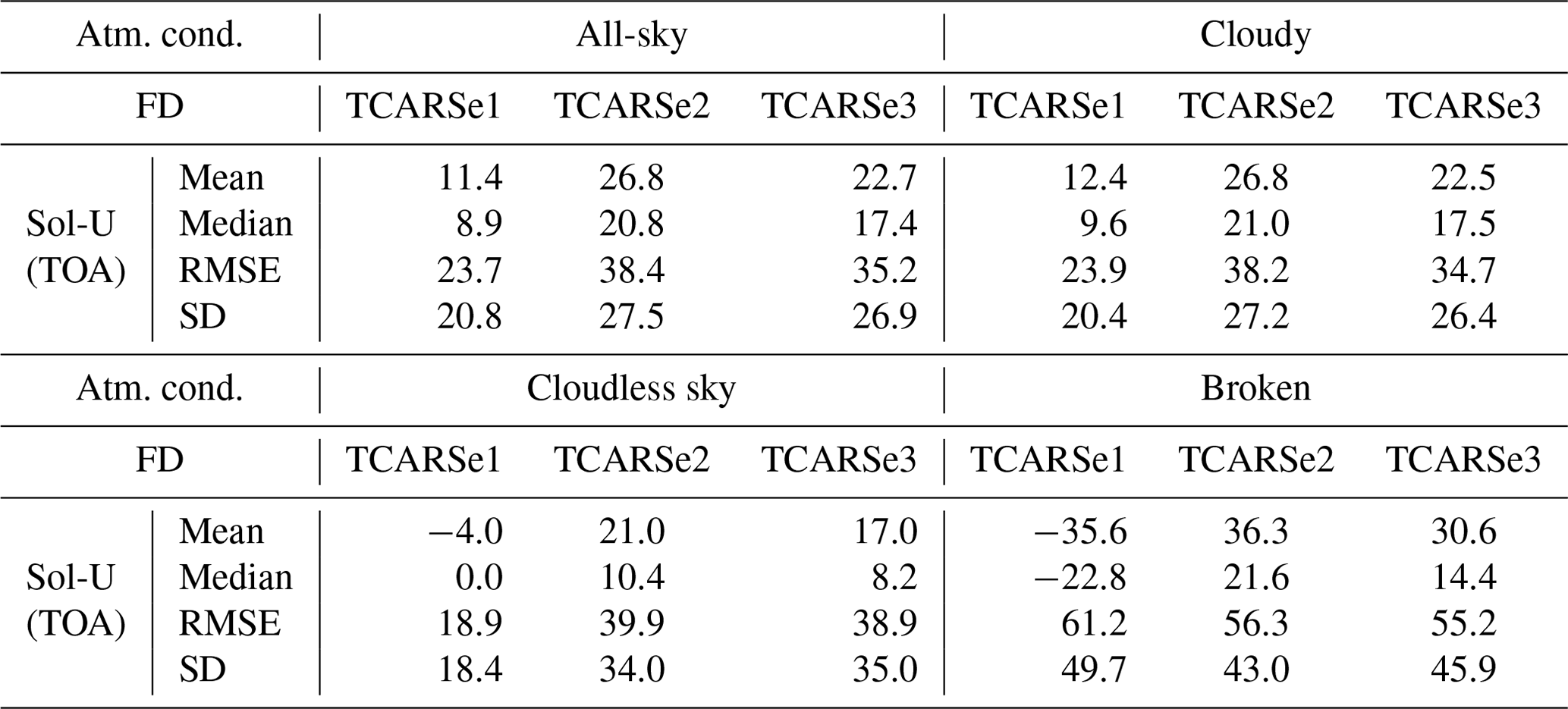
Table 5 Hourly upwelling solar flux (Sol-U) difference (FD) at the top of the atmosphere (TOA) for the entire MOSAiC period under different atmospheric conditions in W m⁻². Results are shown for TCARS simulations using different surface albedo levels based on CERES SYN surface albedo (TCARSe1) and the daily mean from observations at ASFS-30 (TCARSe2) and at ASFS-50 (TCARSe3). An additional comparison for CERES SYN cloudless (CS) products is given for cloudless and broken-cloud conditions.

While the mean Terr-U differences are similar across all stations, ranging from −4.4 to −0.4 W m⁻², the KDE distribution indicates the best agreement above the Met City location. At the AFSF-30 and ASFS-50 sites, a higher occurrence of positive values is observed, whereas the ASFS-40 site shows a greater frequency of negative values (see the first column in Fig. 5). Despite these differences in distribution, the values suggest consistency among TCARSe2 simulations, indicating a limited influence of spatial variability (Fig. D3a). Analysis of single-layer liquid, ice, and mixed-phase clouds shows biases lower than 7.5 W m⁻², confirming the consistency of Terr-U in the TCARS results at the TOA (Table A1).

The comparison of Sol-U comprises all the versions of TCARS simulations. Given that the surface albedo observed at the MOSAiC SO is higher than that of CERES SYN (see Fig. B3; Huang et al., 2022), larger Sol-U fluxes are calculated at the TOA for TCARSe2 and TCARSe3 (Table 5). The median Sol-U difference is lower in magnitude than the results reported in ST2015, with values ranging between 17.4 and 21 W m⁻² for all-sky and cloudy conditions and monomodal distributions around 0.0 W m⁻² (see Fig. 5, second column).

The change in surface albedo affects the calculated Sol-U fluxes by 15.4 W m⁻² during all-sky conditions and up to 25.0 W m⁻² during cloudless conditions. The latter highlights the masking effect that clouds have on TOA reflectance, as discussed in Sledd and L'Ecuyer (2019). The results in ST2015 are relatively similar to the ones calculated here for Terr-U, but the comparison of Sol-U in ST2015 shows larger median flux differences ranging from −41.3 to −14.4 W m⁻². It is worth noting that the median flux difference for cloudless conditions in ST2015 is −43.1 W m⁻², a considerably larger value that could have been caused by differences in spatial inhomogeneities of surface properties within the satellite spatial resolution in contrast to the single-column radiative transfer calculation in ST2015.

The comparison of TCARS terrestrial and solar upwelling fluxes shows consistent agreement with the CERES SYN observations at the TOA, supporting the reliability of TCARS results as estimates of the radiation budget and cloud radiative effects at MOSAiC. Moreover, the differences observed in radiative closure emphasise the significant role of surface albedo and its spatial scaling when comparing different products.

4.4 Radiation budget

The radiation budget is calculated for the MOSAiC period at the surface and at the TOA, utilising TCARS, CERES SYN datasets, and MOSAiC observations. This section provides both monthly and full-year statistics.

Similarly to the previews section (Sect. 4.3), the analysis of the terrestrial flux considers the TCARSe2, and it is extended to the data availability of TCARSe1. The analysis of solar flux also uses the TCARSe2 simulations, as this dataset is based on observed daily mean surface albedo from ASFS-30 that has better temporal coverage than TCARSe3 (see Sect. 3.2, Fig. A2). The calculation of total fluxes (i.e. net terrestrial flux (Terr-N) plus net solar flux (Sol-N)) is based on the aforementioned datasets. The statistical analysis of observed terrestrial fluxes is primarily based on observations from ASFS-30, except for October 2019, when data from Met City were used due to data availability.

Note that the analysis of Terr-N is based on TCARSe1 due to the good temporal coverage. Note that the analysis using TCARSe2 and TCARSe3 simulations was not made, as the analysis would lead to similar results since the only difference among the three sets of experiments is the surface albedo, and this parameter does not influence the Terr flux.

4.4.1 Analysis at the surface

Terr-N showed large variability with values ranging from around −100 W m⁻² to positive values around 25 W m⁻² and lower variability during July and August when Terr-D and Terr-U at the surface are relatively similar because of generally great cloud fraction values (Figs. 2, 6a, and 7k and i).

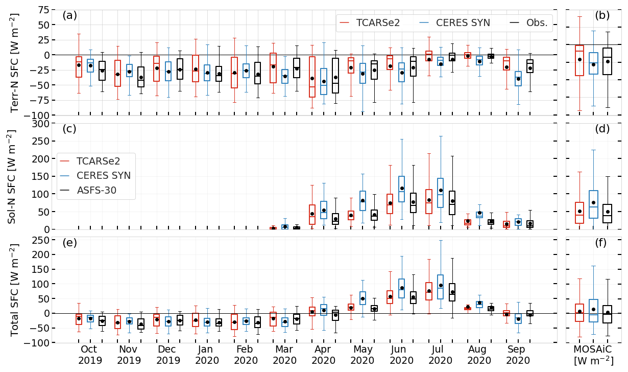
Figure 6 Time series of terrestrial (a, b) and solar (c, d) flux at the surface for TCARS simulations, the CERES SYN product, and observations at the ASFS-30 station and Met City for the last 15 d of October 2019. Panels (e) and (f) show the net radiation budget at the surface (SFC). Panels (b), (d), and (f) show the mean values for the entire MOSAiC period. The box plot shows the distribution of the net fluxes. Panel (d) shows the statistical values for the period when solar radiation is available during MOSAiC. The mean values for the entire MOSAiC expedition are indicated in Table 6.

Table 6 Mean hourly values of the radiation budget and CRE during the entire MOSAiC period in W m⁻². Values in parentheses indicate the standard deviation (SD). The percentage is given for the temporal coverage of the available simulations for MOSAiC. The calculations of the observations (Obs.) are based mostly on ASFS-30 observations, except for October 2019, when the observations at Met City are considered due to temporal coverage. Two calculations are considered for CERES SYN, the first one for 100 % temporal coverage as in TCARSe1 and then for 97.2 % of the same temporal coverage as the TCARSe2 simulations.

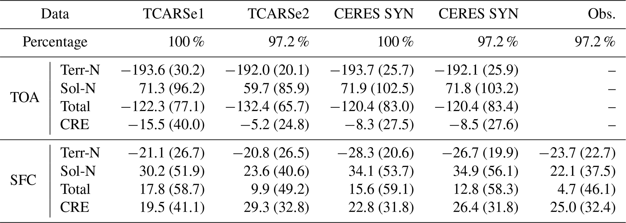
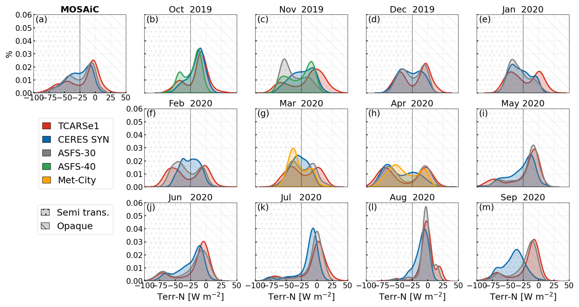
Figure 7 Monthly distributions of net terrestrial flux (Terr-N) at the surface for TCARSe1 simulations, the CERES SYN product, and observations at the ASFS-30 station. For October and November 2019, an additional comparison is shown with observations at ASFS-40, and for March and April 2020, the Terr-N distributions at Met City are included. Note that the distributions in November 2019 and September 2020 represent 15 and 20 d, respectively.

The solar flux at the surface is shown in Fig. 6c and d. The box plots for TCARSe2 and ASFS-30 exhibit relatively similar patterns across all months. In contrast, the CERES SYN data show a clear overestimation of Sol-N, primarily due to lower surface albedo values considered in CERES SYN. With an underestimation of surface albedo by −21.01 % (Huang et al., 2022), the even higher solar flux suggests an underestimation of atmospheric opacity, as more radiation is absorbed by the surface based on the CERES SYN product. The Sol-N values for TCARSe2, CERES SYN, and ASFS-30 are 23.6, 34.1, and 22.1 W m⁻², respectively, indicating that TCARSe2 provides a better representation of the observed Sol-N than the CERES SYN products for the MOSAiC period (Table 6).

The total flux at the surface shows consistent dominance of the Terr flux for most of the year through March 2020 (Fig. 6e). April is the transition month where the values start to become positive. From May to August 2020, the net fluxes at the surface are dominated by the Sol fluxes. The first 20 d of September 2020 is also part of a transition mode, where the net fluxes are near 0 W m⁻². The total flux at the surface for the MOSAiC period based on TCARS, CERES SYN, and observations is 9.9, 15.6, and 4.7 W m⁻², respectively. The overestimation of the total flux from CERES SYN is led by Sol-N by 27.4 W m⁻², whereas the underestimation in Terr-N accounts for 3.0 W m⁻². Using the derived surface albedo from CERES SYN and ShupeTurner retrievals (i.e. TCARSe1) suggests an overall overestimation of the total net flux by 13.9 W m⁻² (Table 6).

Complementarily to the box plots shown in Fig. 6a and b, we include the KDE distribution for the entire MOSAiC period and for each month (Fig. 7). This plot is included to deepen the understanding of the radiation budget and further investigate the variations in Terr-N during MOSAiC.

Figure 7 shows the Terr-N monthly distribution for TCARSe1. The overall comparison for the entire MOSAiC period is shown in Fig. 7a. The remaining panels provide the distribution for each month. Each distribution is subdivided into two zones. Values greater than −25 W m⁻² represent an optically thick atmosphere, and values less than −25 W m⁻² are defined as a semi-transparent atmosphere.

Additionally, for October and November 2019, the distribution from ASFS-40 (green) is included, and for March and April 2020, the observations at Met City are added (orange). The observations at these stations were added as the observations had more hourly data samples compared to observations at ASFS-30. The comparison of TCARSe1 and the CERES SYN product was limited to the data availability of the observations, meaning that if there were any data gaps, the exact hourly sample was removed from TCARSe1 and CERES SYN datasets for a fair comparison. For October and November 2019, the data were limited to the data coverage of ASFS-40 observations, and for March and April, the datasets were limited to the data availability at Met City. The rest of the months were limited to the observations at ASFS-30.

Based on the Terr-N comparison for the entire MOSAiC period, the atmosphere was characterised by a bimodal distribution in all seasons, indicating distinct occurrences of optically opaque and optically thin atmospheres. However, for the months of May through September, there is a particularly frequent occurrence of optically thick atmospheres, consistent with the frequent occurrence of clouds with high LWP in these months (Fig. 3a). In October 2019, the last 15 d of the month was analysed, and in September 2020, the first 20 d was evaluated, showing relatively similar distributions of Terr-N and indicating a higher occurrence of opaque atmospheres.

The TCARSe1 Terr-N distribution generally captures the bimodal distribution observed for most months, although discrepancies arise during polar-night months, when it tends to overestimate the occurrence of the highest-opacity cases and underestimate the occurrence of low-opacity cases compared to observations.

The CERES SYN Terr-N distributions exhibit considerable discrepancies with both the observed data and TCARSe1 simulations, particularly in the shapes of the KDE distributions, which generally indicate optically thinner atmospheres, as discussed in Sect. 4.3.1 and previously noted in Huang et al. (2022). Another explanation might be related to the spatial resolution that could smooth out the clear differences between an opaque and semi-transparent atmosphere. The more negative Terr-N values are especially pronounced during the polar night. In contrast, during the polar day, the distributions align more closely with observations. This finding is consistent with Fig. 2, which shows that the months with the greatest discrepancies occur when the frequency of CERES SYN cloud fraction is lower than that of the ShupeTurner retrievals.

In February 2020, the CERES SYN Terr-N KDE distribution indicated a more frequent occurrence of semi-transparent atmospheres. This resulted in an overestimation of cloudless conditions and an underestimation of atmospheric opacity. A detailed analysis of several cases in this month and during September indicated a more frequent underestimation when the cloud base was misidentified during snow precipitation events identified by ShupeTurner (not shown).

September 2020 poses a particularly challenging comparison, as the Terr-N discrepancy stems not only from an underestimation of cloud opacity but also from a significant underestimation of skin temperature, leading to an underestimation of Terr-U values in the CERES SYN product (see Fig. B2). A comparison using observed Terr-U fluxes at ASFS-30 instead of Terr-U fluxes from CERES SYN indicates a higher distribution toward a more semi-transparent atmosphere (not shown), making September 2020 the period with the most pronounced underestimation of cloud opacity by CERES SYN. It is worth clarifying that from 4 to 19 September, ASFS-30 was positioned over a re-freezing melt pond (Cox et al., 2023e), which may also explain these differences.

4.4.2 Analysis at the TOA

Figure 8a illustrates the monthly Terr-N at the TOA, showing a consistent annual variation between TCARSe1 and CERES SYN and indicating less negative values of the outgoing terrestrial radiation during the polar night in contrast to the polar day, as more radiation is emitted from the surface through the atmosphere to the TOA due to warmer and more humid conditions. The mean Terr-N for TCARSe1 and CERES SYN is −193.6 and −193.7 W m⁻², respectively (Table 6, Fig. 8b).

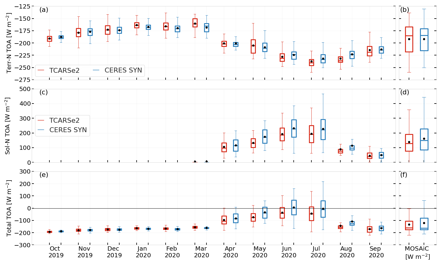
Figure 8 Time series shown as monthly box plots for the (a, b) net terrestrial flux (Terr-N), (c, d) net solar flux (Sol-N), and (e, f) total flux at the top of the atmosphere (net). The box plots for TCARS are displayed in red, while the ones for CERES SYN are shown in blue. Box plots for the entire MOSAiC period are displayed in panels (b), (d), and (f). Panel (d) shows the statistical values for the period when solar radiation is available during MOSAiC. The mean values for the entire MOSAiC expedition are indicated in Table 6.

The comparison of Sol-N is depicted in Fig. 8c and d. TCARSe2 calculations exhibit a consistent variation compared to CERES SYN calculations, reaching the highest values in July 2020 and then decreasing in magnitude and variability as a result of decreased surface albedo until September 2020. This behaviour is due to the interactions of clouds with a lower surface albedo and lower sun elevations for this period of the year. The mean Sol-N at the TOA for TCARSe2 is 59.7 W m⁻², while for CERES SYN, the mean value is 71.8 W m⁻². This indicates that the surface–atmosphere system in TCARSe2 simulations absorbs more solar radiation due to greater atmospheric opacity. This increased opacity inhibits a significant amount of solar flux from reaching the surface, resulting in a lower solar flux (Sol-U) reaching the TOA (see Table 6, Fig. 8d).

At the TOA, the radiation budget is predominantly influenced by the Terr flux for the majority of the MOSAiC period, as depicted in Fig. 8e, with the exceptions being June and July. The net radiation at the TOA, calculated using TCARS and CERES SYN observations, is −92.7 and −105.7 W m⁻², respectively. The discrepancy between these values is primarily attributed to differences in the Sol flux, whereas the Terr fluxes exhibit better agreement.

4.5 Cloud radiative effect

Similarly to Sect. 4.4, the cloud radiative effect is presented in both monthly and full-year statistics. The calculation of the CRE at the SFC and at the TOA considers Eq. (1) and is displayed in Figs. 9 and 10, respectively. Additionally, the analysis at the SFC considers the hybrid calculation of the CRE by considering the TCARSe2 cloudless simulations and the observations of upwelling and downwelling Sol and Terr fluxes at ASFS-30 (shown in black in Fig. 9).

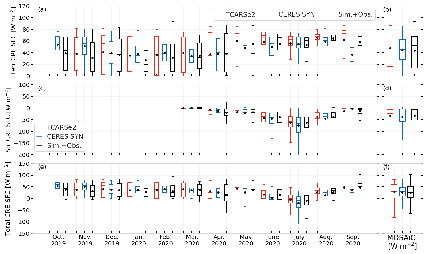
Figure 9 Time series of monthly box plots for the terrestrial (a), solar (c), and total (e) cloud radiative effect (CRE) at the surface. Box plots for the entire MOSAiC period are shown in panels (b), (d), and (f). Panel (d) shows the statistical values for the period when solar radiation is available during MOSAiC. The mean values for the entire MOSAiC expedition are indicated in Table 6.

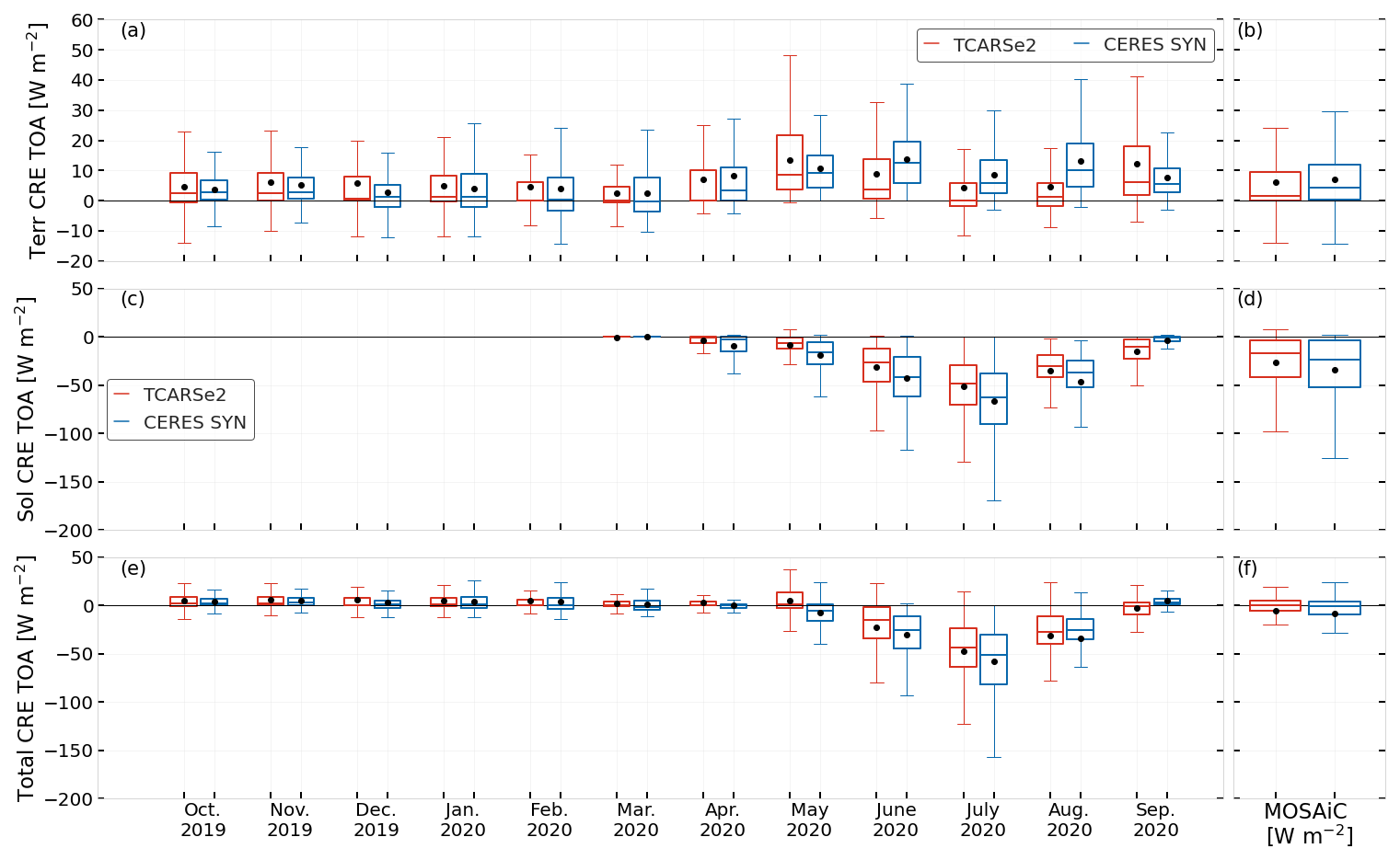
Figure 10 Time series of monthly box plots of the terrestrial (a), solar (c), and net (e) cloud radiative effect (CRE) at the TOA. Box plots for the entire MOSAiC period are shown in panels (b), (d), and (f). Panel (d) shows the statistical values for the period when solar radiation is available during MOSAiC. The mean values for the entire MOSAiC expedition are indicated in Table 6.

The distribution of the Terr CRE shows lower values during the polar night and larger values for October 2019 and from May to September 2020. The annual variation in the Terr CRE is consistent with the findings reported at other sites like the SHEBA (Surface Heat Budget of the Arctic Ocean) expedition carried out from 1997 to 1998 north of Alaska (Intrieri et al., 2002; Shupe and Intrieri, 2004), in Ny-Ålesund (Ebell et al., 2020), at the ARM NSA site and NOAA Barrow Observatory in Utqiaġvik (Dong et al., 2010), and in Greenland at Summit Station (Miller et al., 2015).

Additional attention should be given to September 2020, as the largest CERES SYN discrepancies are found during this month. Terr-D is notably underestimated (see Fig. 6a) and does not align with the atmospheric opacity indicated by the other datasets (refer to Fig. 7m).

The biggest difference among the mentioned sites is that the monthly Terr CRE means at the two Utqiaġvik sites (Dong et al., 2010) are the lowest in March, with values around 10 W m⁻², contrasting the lowest mean values around 30 W m⁻² calculated in this study and at the other sites. These differences stem from the particular characteristics at each site (Shupe et al., 2011). It is important to note that this comparison aims to provide a general context for the observations at other sites rather than a direct comparison, as the data sampling periods and the number of data considered differ. Additionally, some discrepancies are due to differences in how the equivalent clear-sky reference was calculated (Dong et al., 2010).

The calculation of Sol CRE shows a consistent increase in magnitude as there is more solar radiation during June and July 2020 at MOSAiC (Fig. 9c). It is noteworthy that positive values are observed for the hybrid calculations, as broken-cloud conditions are not excluded from this analysis. These conditions cannot be simulated within the 1D radiative transfer setup of TCARS and CERES SYN; hence the values from these models cannot be positive.

Stapf et al. (2020) argued that the calculation of the solar cloud radiative effect should be reassessed by distinguishing between the roles of cloudless and all-sky surface albedo. They discuss the applicability of a broadband parameterisation that considers the presence of liquid clouds. Based on aircraft observations, Jäkel et al. (2024) additionally considered the impact of surface type including snow coverage and the melt-pond fraction, and they compared these observations to the surface albedo scheme of an atmospheric model. Understanding how factors such as surface type, the solar zenith angle, and cloud properties including the thermodynamic phase of clouds influences broadband surface albedo is important but beyond the scope of the current work.

At the TOA, the variation in the terrestrial CRE is determined by the cloud top temperature relative to the inversion top temperature. A warming effect is associated with high-level clouds, while a cooling effect occurs when the cloud top temperature is similar to the top atmospheric inversion temperature, a condition more common with mid- and low-level clouds. May and June had the highest cloud occurrence during MOSAiC (Fig. 2), resulting in one of the highest mean Terr CRE values at the TOA, around 10.0 W m⁻² (Fig. 10a). The mean Terr CRE for the entire MOSAiC period is 6.5 and 7.0 W m⁻² for TCARSe2 and CERES SYN, respectively.

The Sol CRE at the TOA shows lower values for TCARSe2 in comparison to CERES SYN. The coolest CRE occurs in July, with mean values of −51.2 and −67 W m⁻² for TCARSe2 and CERES SYN, respectively (Fig. 10b). The mean Sol CRE for the MOSAiC period is −26.9 W m⁻² for TCARSe2 and −34.2 W m⁻² for CERES SYN.

The total CREs at the SFC and TOA are shown in Figs. 9e and f and 10e and f, respectively. The time series shows a dominance of warming CRE at the SFC for most of the months except for July 2020 at the SFC and for June, July, and August 2020 at the TOA. For the entire MOSAiC period, the total CRE at the SFC based on TCARS, CERES SYN, and hybrid calculations is 29.3, 26.4, and 25.0 W m⁻², respectively (Table 6). At the TOA the total CRE is dominated by the cooling effect of −5.2 W m⁻² based on TCARSe2 calculations and of −8.5 W m⁻² based on CERES SYN (Table 6, Fig. 10e and f). The latter indicates that during MOSAiC, the atmosphere–surface system loses 5.2 W m⁻² to space while the surface gains 25.0 W m⁻² due to the presence of clouds leading to a cooling of the atmosphere by 30.2 W m⁻².

5 Summary, conclusions, and outlook

This study analysed the radiation budget and cloud radiative effect during the MOSAiC expedition. The accuracy of ShupeTurner cloud products, based on passive and active remote sensing observations, was indirectly evaluated through radiative closure studies. These retrievals served as input parameters for a single-column radiative transfer to obtain a dataset of simulated radiative flux profiles.

The simulated fluxes were compared to observations of broadband upwelling and downwelling solar and terrestrial radiative fluxes measured at different stations located over the ice floe and collocated satellite products from CERES SYN Ed. 4. Our results indicate that, in general, there is overall agreement among the simulations, CERES SYN data, and ice-floe observations, supporting our analysis of the radiation budget and cloud radiative effects during the MOSAiC expedition.

In addition, we evaluated three experiments of the TCARS simulations using different sources of surface albedo as input parameters to constrain the surface–cloud–radiation interaction and its effect on Sol-D.

Guided by the research questions proposed in the Introduction, we summarise our findings and conclude the following:

1. The cloudless TCARS- and CERES SYN-simulated results exhibit good agreement for Terr and Sol fluxes at both the surface and the TOA. The results suggest a consistent correlation across seasons, with correlation coefficients greater than 0.87. However, more notable differences in mean downwelling fluxes are observed for Sol-D during summer months, displaying a mean flux difference of up to 7.2 W m⁻². This discrepancy is attributed to the presence of aerosols, as a comparison using pristine CERES SYN product reduces the bias to −2.0 W m⁻².

2. Overall comparisons between TCARS and MOSAiC flux observations indicate relatively good agreement for all-sky, cloudy, and cloudless conditions, with median flux differences that do not exceed ±4.8 W m⁻² for Terr-D and ±6.8 W m⁻² for Sol-D.

   The comparison of CERES SYN fluxes to MOSAiC observations also suggests good agreement for Terr-D and Sol-D, with hourly median flux differences not exceeding 10.2 W m⁻². However, in contrast to the TCARS results, the CERES SYN comparison displays negative and positive biases for Terr-D and Sol-D, respectively. This suggests a plausible underestimation of cloud optical thickness, as previously suggested by Huang et al. (2022).

3. Having several ground-based observations of radiative fluxes over the ice floe covering areas of up to approximately 20 km (Cox et al., 2023e) aids the analysis of spatial-scale differences between a shipborne measurement and a satellite footprint or grid product. This analysis revealed that Terr-D did not exhibit large variations among Met City, ASFS-30, ASFS-40, and ASFS-50 observations, corroborating the findings in Rabe et al. (2024). On the other hand, other flux components were susceptible to larger differences, especially under cloudless conditions, when the Sol-U fluxes varied by up to 15 W m⁻². This indicates that the spread among sites was large enough to capture small-scale spatiotemporal variability in the surface conditions. Moreover, all of these surface observations were made over sea ice and thus do not capture the variability in albedo on larger scales that include some contributions from leads.

4. Evaluating Terr-N at the surface provides an approximation of atmospheric opacity. In winter, atmospheric conditions show a bimodal distribution, while summer is characterised by optically thick clouds. Comparing Terr-N helped identify periods when cloud opacity estimates caused biases in TCARS and CERES SYN products.

   CERES SYN often underestimates cloud opacity during snowfall events, particularly in the polar-night season, likely due to misidentifying the cloud base with temperatures lower than observed. In contrast, TCARS tends to overestimate cloud opacity with geometrically thick ice clouds, possibly due to using retrieval coefficients developed for other Arctic areas (Shupe et al., 2005), which may not be suitable for MOSAiC. Nonetheless, the closure statistics presented here are quite similar to those achieved for a different time period at the NSA site (Shupe et al., 2015), suggesting a general consistency of the ShupeTurner product and the radiative closure framework.

5. The surface radiation budget during MOSAiC indicated a clear dominance of the terrestrial flux for most months with the exception of May, June, July, and August. A relatively similar distribution of Terr-N is observed for the TCARS, CERES SYN, and MOSAiC observations, with values ranging from −20.8 to −28.3 W m⁻². The mean Sol-N for the MOSAiC period ranged from 22.1 to 34.9 W m⁻². Results of the yearly cycle of the net and downwelling fluxes are comparable to previous results shown in Intrieri et al. (2002), Dong et al. (2010), Miller et al. (2015), and Ebell et al. (2020) for the sites of SHEBA, Summit in Greenland, Alaska, and Ny-Ålesund, respectively.

6. The analysis of total CRE at the surface using TCARS, CERES SYN, and a hybrid approach showed good agreement, indicating a warming effect of clouds between 19.5 and 30.6 W m⁻². Throughout the year, TCARS and hybrid calculations aligned well, though TCARS showed higher CRE values during the polar night, possibly due to overestimating ice cloud opacity from ShupeTurner retrievals. CERES SYN products have a similar mean and median Terr CRE to the hybrid calculation, but this is likely compensated for by a less humid and colder cloudless atmosphere utilised in CERES SYN to simulate the radiative fluxes at the surface. Overall, results were consistent with earlier studies (Intrieri et al., 2002; Shupe and Intrieri, 2004; Dong et al., 2010; Miller et al., 2015; Ebell et al., 2020) but differed based on unique atmospheric and surface conditions.

Future work should focus on the representation of and variability in surface albedo across different scales, as radiative fluxes and cloud radiative effects are sensitive to these influences. It is essential to quantify the spatiotemporal variability from shipborne measurements to satellite footprints, building on findings from this paper as well as Huang et al. (2022) and Jäkel et al. (2024). We also recommend analysing differences in CERES SYN using a reanalysis product that incorporates radiosondes from MOSAiC, as GEOS-5.4.1 may reflect a less humid, colder Arctic atmosphere during the polar night. Lastly, we aim to deepen the analysis of atmospheric processes related to heating rates and expand the climatological relevance of these findings by including other Arctic locations like Ny-Ålesund.

Appendix A: Radiative transfer simulations

Additional illustrations showing the methodology of the radiative transfer simulations using the TCARS framework (Fig. A1) and the temporal coverage of the different radiative transfer experiments created with TCARS (Fig. A2).

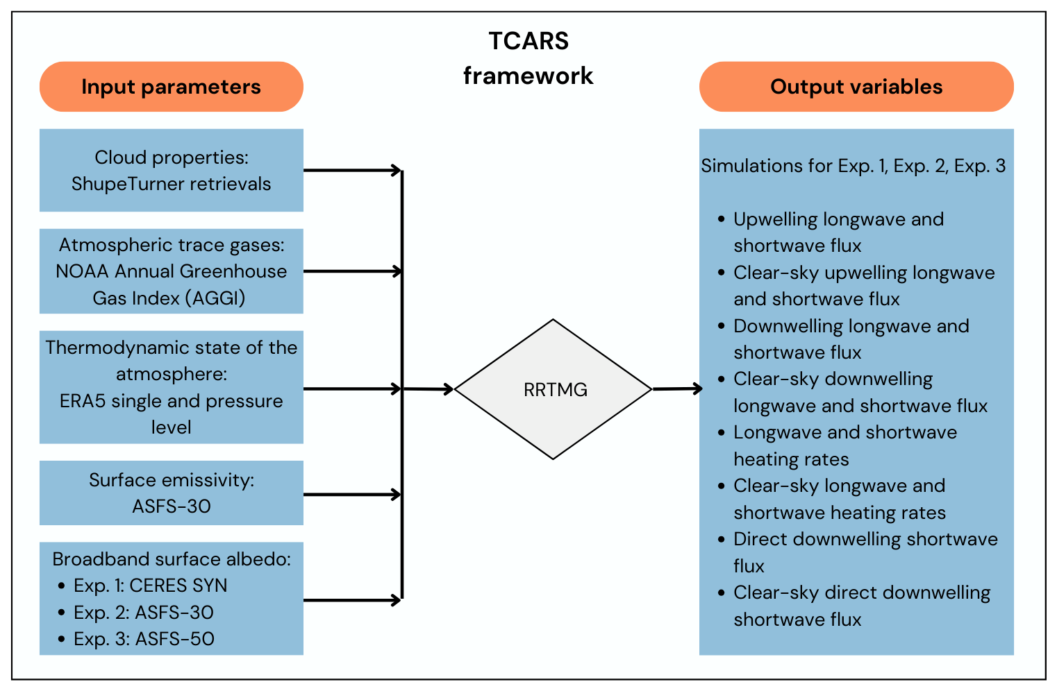
Figure A1 Flow chart showing the steps followed to obtain the radiative transfer simulations using the TCARS framework. The naming of output variables is given according to the dataset variable naming in Barrientos-Velasco (2024), referring to the solar fluxes as shortwave and to the thermal fluxes as longwave.

Table A1 The hourly radiative flux difference (FD) between simulated (TCARSe1) and observed downwelling fluxes at the surface (SFC) and upwelling fluxes at the top of the atmosphere (TOA) for single-layer clouds subdivided by cloud phase for the entire MOSAiC period in W m⁻². The flux comparison at the surface considers observations at the ASFS-30 station and the TOA products from CERES SYN. In parentheses is given the frequency of occurrence of the different single-layer cloud types. Precipitating events accounted for 20 % of the time.

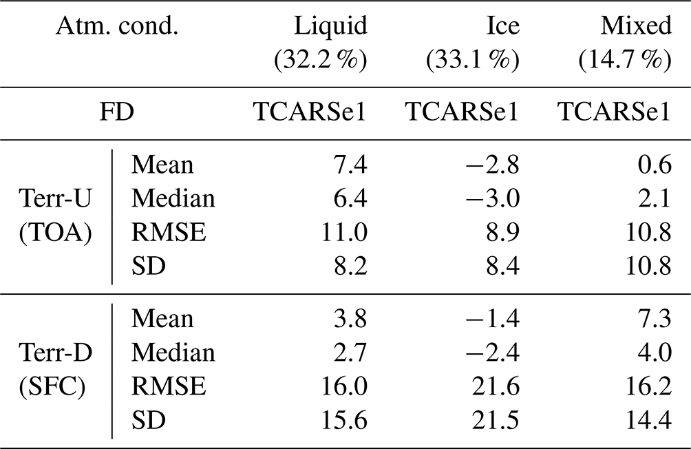
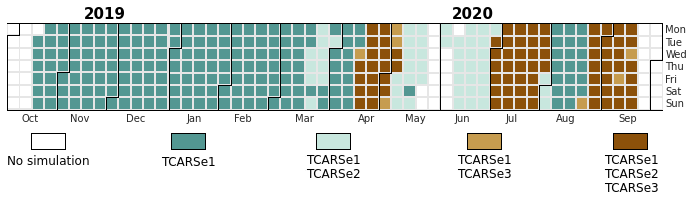
Figure A2 Heat map plot showing the temporal coverage of each experimental set of TCARS simulations for the MOSAiC period from 15 October 2019 to 20 September 2020.

Table A2 The hourly radiative flux difference (FD) between TCARS and observations measured in W m⁻². At the surface (SFC), downwelling fluxes are compared, while at the top of the atmosphere (TOA), solar upwelling fluxes are analysed. These comparisons are conducted for single-layer clouds, which are further subdivided by cloud phase, over the entire MOSAiC period. Surface observations are obtained from the ASFS-30 station, and TOA observations are sourced from CERES SYN data. TCARS simulations using different surface albedo data sets based on CERES SYN surface albedo (e1) and the daily mean from observations at ASFS-30 (e2) and at ASFS-50 (e3). In parentheses is given the frequency of occurrence of the different single-layer cloud types. Precipitating events accounted for 22.7 % of the time.

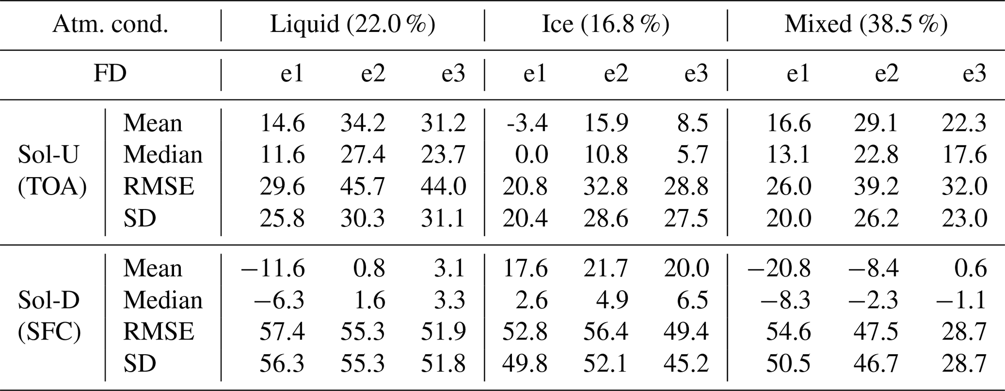
List of abbreviations

Abbreviation	Meaning
AGGI	Annual Greenhouse Gas Index
Atm.	Atmospheric
ASFS	Atmospheric surface flux station
CERES	Clouds and the Earth's Radiant Energy System
CERES SYN	Clouds and the Earth's Radiant Energy System SYN Ed. 4.1 product
Cond.	Conditions
CS	Cloudless
CRE	Cloud radiative effect
Eff.	Effective
FD	Flux difference
KDE	Kernel density estimate
LWC	Liquid water content
LWP	Liquid water path
MOSAiC	Multidisciplinary drifting Observatory for the Study of Arctic Climate
Net CRE	Net cloud radiative effect (terrestrial plus solar CRE)
IWC	Ice water content
IWP	Ice water path

Obs.	Observations
PS	Polarstern
rE, L	Liquid droplet effective radius
rE, I	Ice crystal effective radius
RMSE	Root mean squared error
RRTMG	Rapid Radiative Transfer Model (RRTM) for GCM applications
SFC	Surface
SO	Surface Observatory
Sol-D	Broadband downwelling solar (shortwave) flux
Sol-N	Broadband net solar (shortwave) flux
Sol-U	Broadband upwelling solar (shortwave) flux
SD	Standard deviation
TCARS	TROPOS Cloud and Aerosol Radiative effect Simulator
Terr-D	Broadband downwelling terrestrial (longwave) flux
Terr-N	Broadband net terrestrial (longwave) flux
Terr-U	Broadband upwelling terrestrial (longwave) flux
TOA	Top of the atmosphere
Total flux	Terr-N plus Sol-N

Appendix B: Atmospheric and surface conditions

The atmospheric temperature during MOSAiC is illustrated in Fig. B1 based on ERA5 atmospheric profiles and the blended product from Dahlke et al. (2023) to illustrate the variation in this parameter in kelvins (K).

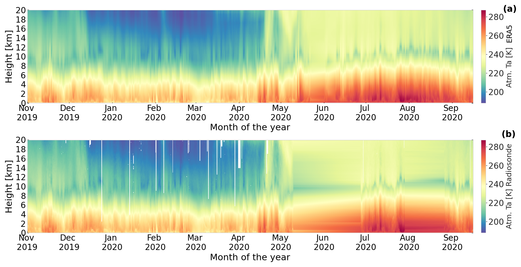
Figure B1 Time series of linearly interpolated atmospheric temperature for MOSAiC based on ERA5 (a) and merged radiosondes (b).

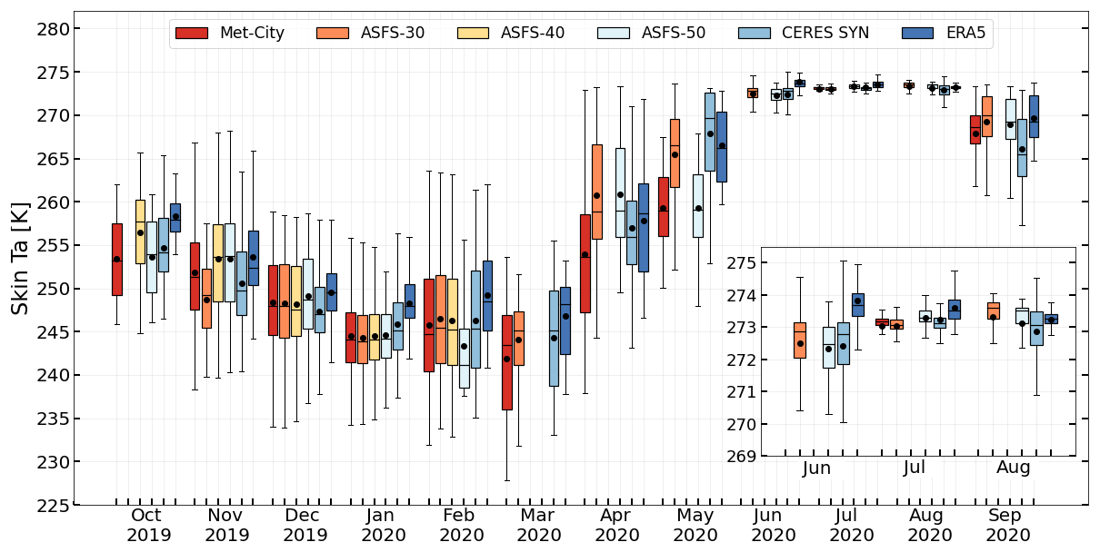
Figure B2 Monthly time series of box plots showing the distribution of skin temperature for MOSAiC based on ERA5, CERES SYN, and ice-floe stations.

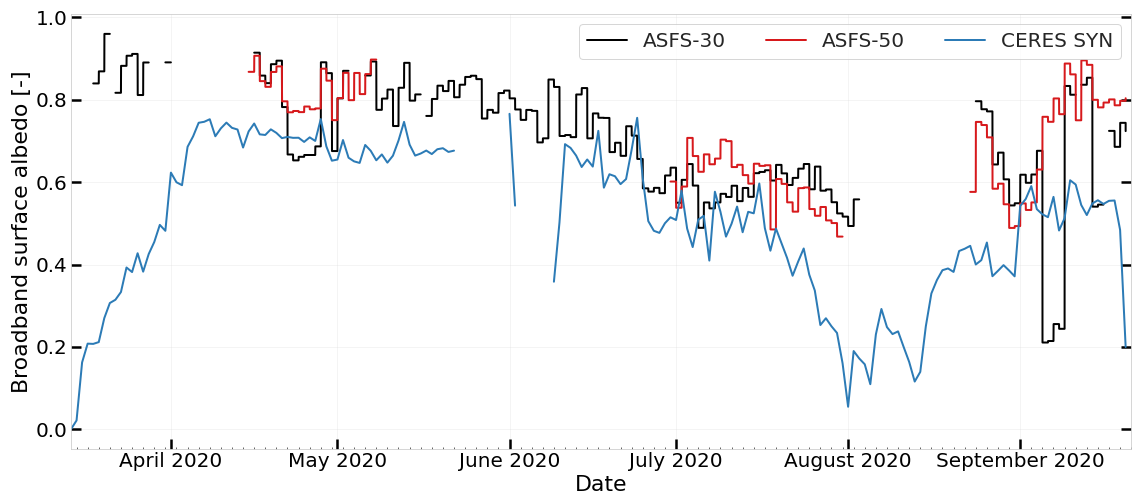
Figure B3 Time series of the daily mean broadband surface albedo from 14 March to 20 September 2020. Data gaps in the CERES SYN time series are subject to the overall data availability for the radiative transfer simulations.

Appendix C: Comparison of cloudless simulations

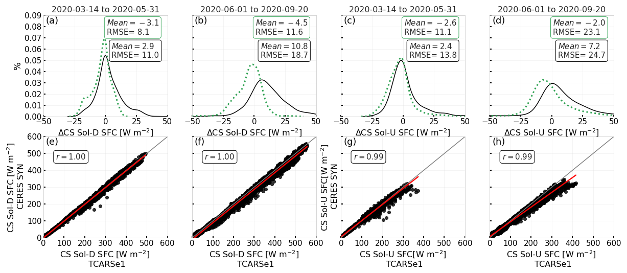
Figure C1 Comparison of (a, b, e, f) downwelling solar radiative flux (Sol-D) and (c, d, g, h) upwelling solar radiative flux (Sol-U) at the surface for cloudless simulations between TCARS and CERES SYN: the first row shows the kernel density estimate (KDE) distribution of TCARS minus CERES SYN fluxes, and the second row shows scatter plots comparing CERES SYN (y axis) and TCARS simulations (x axis). Linear regressions are shown by the red line. The mean, RMSE, and correlation coefficient are indicated in the panels. Each column depicts the results for each period indicated in the top panel. The dotted green KDE distribution shown in panels (a)–(d) shows the same comparison for CERES SYN fluxes for pristine conditions.

Appendix D: Radiative flux difference for all available ice-floe stations during MOSAiC

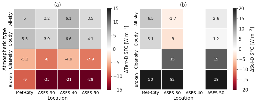
Figure D1 Mean flux difference between TCARSe1 simulations and observed broadband radiative fluxes for MOSAiC at the surface (SFC). Panels (a) and (b) show downwelling terrestrial flux (Terr-D) and solar flux (Sol-D), respectively, for all stations.

Figure D2 The same as Fig. D1 but comparing CERES SYN minus observations.

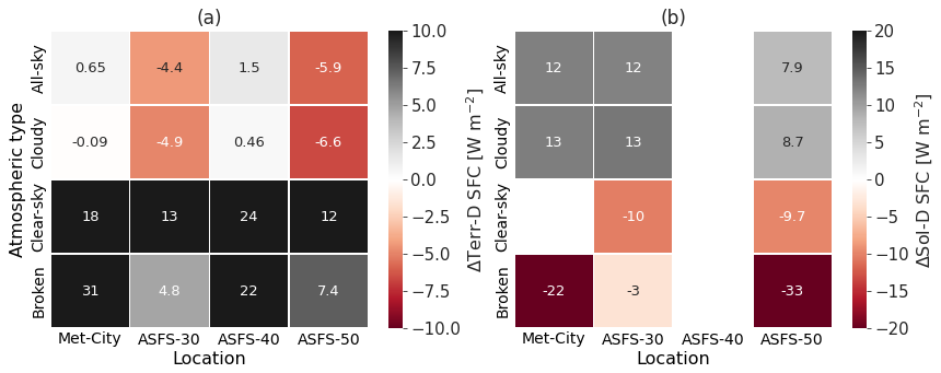
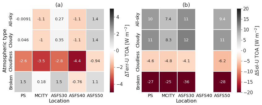
Figure D3 Mean flux difference between TCARS and CERES SYN fluxes at the TOA. Panel (a) shows biases for the upwelling terrestrial flux (Terr-U) considering TCARSe1, and panel (b) shows the comparison for the upwelling solar flux (Sol-U) using TCARSe2.