Hygroscopic aerosols amplify longwave downward radiation in the Arctic

This study investigates the impact of hygroscopic aerosols, such as sea salt and sulfate, on longwave downward radiation in the Arctic. These aerosols absorb atmospheric water vapor, leading to wet growth, increased size, and enhanced longwave downward radiation emission, defined as the aerosol infrared radiation effect. Observations of aerosols, especially their composition, are challenging during the Arctic winter. We use an emission Fourier transform spectrometer to measure aerosol composition. Observations show that the aerosol infrared radiation effect of dry aerosols is limited to about 1.45±2.00 W m⁻². Wet growth significantly increases this effect. During winter, at relative humidity levels between 60 % and 80 %, wet aerosols exhibit effects approximately 7 times greater than dry aerosols. When relative humidity exceeds 80 %, the effect can be up to 20 times higher. Sea salt aerosols in Ny-Ålesund demonstrate high effect values, while non-hygroscopic aerosols like black carbon and dust show consistently low values. Reanalysis data indicate increased water vapor and sea salt aerosol optical depth in Ny-Ålesund after 2000, correlating with significant positive temperature anomalies in this area. Moreover, wet aerosols can remain activated even in dry environments, continuously contributing high effects, thereby expanding the area affected by aerosol-induced warming. This warming effect may exacerbate Arctic warming, acting as a positive feedback mechanism.

1 Introduction

Arctic amplification, characterized by the accelerated warming of the Arctic region compared to global averages, is a phenomenon of importance in climate change (Serreze and Barry, 2011; Wendisch et al., 2017; Peace et al., 2020). This amplified warming is particularly pronounced during the polar night, highlighting the need for a comprehensive understanding of its causes and consequences (Chung et al., 2021). To elucidate the underlying mechanisms driving Arctic amplification, extensive research has focused on key processes such as temperature feedback, surface albedo feedback, and cloud and water vapor feedback (Bony et al., 2006; Soden and Held, 2006; Graversen et al., 2014; Taylor et al., 2013; Philipp et al., 2020). Among these, aerosols are an important factor in Arctic climate dynamics, influencing various feedback mechanisms. For instance, dust and black carbon (BC) depositions on snow or ice surfaces reduce albedo, accelerating ice melt (Ming et al., 2009; Bond et al., 2013). Moreover, sea salt aerosols modify cloud properties, enhancing longwave downward radiation (LWD) and contributing to surface warming (Gong et al., 2023).

In the context of the Arctic energy budget, LWD constitutes a critical component, primarily governed by greenhouse gases (GHGs) in the global mean (Trenberth et al., 2009; Wild et al., 2015; Tian et al., 2023). However, during the polar night when solar shortwave radiation is absent, the cooling effect of clouds and aerosols, arising from the scattering of solar radiation, becomes negligible (Cox et al., 2015). Therefore, LWD from clouds and aerosols assumes greater significance, particularly in maintaining the Arctic energy balance (Serreze and Barry, 2011; Cox et al., 2015; Lenaerts et al., 2017; Ebell et al., 2020). Compared with LWD from clouds (50–100 W m⁻², Serreze and Barry, 2011; Cox et al., 2015; Lenaerts et al., 2017; Ebell et al., 2020), previous studies have shown that the LWD caused by aerosols in dry conditions is usually lower than 10 W m⁻² (Spänkuch et al., 2000; Markowicz et al., 2003; Vogelmann et al., 2003; Lohmann et al., 2010). Dry aerosol particles contribute very limited LWD to the Arctic climate. However, LWD in the transition state (wet aerosols) between dry aerosols and cloud droplets is rarely mentioned.

Aerosols in the atmosphere, including sea salt and sulfates, possess hygroscopic properties, allowing them to absorb water vapor and undergo wet growth (Winkler, 1973). This process, known as aerosol wet growth, is accompanied by an increase in LWD (Mauritsen et al., 2011). The magnitude of this increase is influenced by factors such as aerosol composition and ambient relative humidity (RH) (Peng et al., 2022). Notably, the deliquescence point, at which hygroscopic aerosols abruptly increase in size, is a critical threshold determined by ambient RH (Tang and Munkelwitz, 1993; Winkler, 1973). For example, the sea salt and sulfate aerosols in this study have deliquescence points of about 75 % and 85 %, respectively (Peng et al., 2022). This means that when the ambient humidity increases to 75 %, the dry sea salt aerosol particles can absorb water vapor in the atmosphere and become larger. If the ambient humidity continues to increase, the sea salt wet particles will continue to absorb water and become sea salt solution droplets (still belonging to aerosols). This is the wet growth process of sea salt aerosols. Recent studies have shown an increase in Arctic water vapor content, attributed to enhanced poleward transport facilitated by atmospheric river pathways (Sato et al., 2022; Thandlam et al., 2022; Bresson et al., 2022; Lauer et al., 2023). Moreover, sea salt aerosols have been identified as dominant contributors to Arctic aerosol composition during the winter season (Huang and Jaeglé, 2017; Kirpes et al., 2018). Therefore, the rise in coarse-mode aerosols, primarily originating from sea spray, and the increase in RH in the Arctic underscore the need to investigate the potential impact of aerosols on LWD and Arctic warming during their wet growth process (Heslin-Rees et al., 2020; Pernov et al., 2022).

Given the complex interplay between aerosols (especially aerosol composition), RH, and LWD, understanding the radiative effects of aerosol wet growth is crucial for understanding the role of aerosols in Arctic amplification, particularly during the polar night. Considering the various factors contributing to atmospheric LWD, such as greenhouse gases, clouds, and aerosols, this study aims to explore the extra LWD introduced during aerosol wet growth. Thus, we focus on hygroscopic aerosols, particularly sea salt and sulfate aerosols. Our study focuses on humidity levels below 100 %, meaning we only discuss aerosols in their dry and wet states. We take aerosol in RH <60 % as dry states. When the environment becomes more humid (RH >60 %), a hygroscopic particle can absorb water, and its size grows, which can act as cloud condensation nuclei (CCN). This hygroscopic particle is defined as wet aerosol in our study. To achieve this, both model simulations and observational data (site location: Ny-Ålesund; time period: December–January–February, 2017–2022) are utilized, defining the resulting additional LWD from aerosols as the aerosol infrared radiation effect (ARE). This paper is structured as follows: Sect. 3 provides an overview of the datasets utilized, including Fourier transform infrared spectroscopy and Baseline Surface Radiation Network (BSRN) measurements. Section 4 outlines the methodologies employed to derive ARE from LWD measurements (eliminating contributions from clouds and GHGs) in detail. The results are presented in Sect. 5. Finally, the implications of these findings are discussed in the conclusion (Sect. 7).

2 Site description

Ny-Ålesund (78.925° N, 11.925° E), Svalbard, is located in the North Atlantic atmospheric transport gateway to the Arctic. It serves as a central hub for international Arctic research, attracting scientists from around the world to study various environmental and climate-related phenomena, in particular to monitor Arctic amplification. The region stretching from Svalbard to the Barents and Kara seas is currently experiencing particularly intense winter warming, with temperatures rising by more than +3 K per decade (Dahlke and Maturilli, 2017). This region is also an important pathway for air mass transport between the Arctic and mid-latitudes (Graßl et al., 2022). Today, Ny-Ålesund is primarily a research town, hosting several year-round research stations operated by different nations. Key activities focus on long-term atmospheric monitoring, studying the effects of climate change in the Arctic, and tracking the transport of pollutants and aerosols from lower latitudes to the Arctic. Due to its location and concentration of research infrastructure, Ny-Ålesund is a well-known site for Arctic research, providing invaluable data and insights into one of the most rapidly changing regions on Earth.

3 Data

All observations and model simulations in this study are conducted in Ny-Ålesund. The surface radiation measurements; radiosonde launches; and all measurements by cloud radars, microwave radiometers, ceilometers, and Fourier transform spectrometers (FTIRs) are operated at the Atmosphere Observatory of the AWIPEV research base that is run jointly by the German Alfred Wegener Institute and the French Polar Institute. Data from both observations are filtered by using Cloudnet data to ensure cloud-free conditions, focusing solely on aerosols.

The FTIR plays a crucial role in elucidating the relationship between aerosol composition and ARE, offering detailed insights into aerosol composition while quantifying ARE. However, the ARE from the FTIR is restricted to the atmospheric window (AW) region (690–1390 cm⁻¹; 7–14 µm). On the other hand, the BSRN provides LWD data across the entire mid-infrared region (4.5–42 µm) but cannot characterize aerosol composition. Each dataset presents different advantages and limitations. Furthermore, it is essential to account for the influences of other radiative sources, such as clouds and greenhouse gases, to accurately assess ARE.

3.1 Cloud and aerosol signals from Cloudnet

In order to identify cloud cases, the Cloudnet Classification product is used (Illingworth et al., 2007). Cloudnet is operationally applied to the AWIPEV measurement (Nomokonova et al., 2019; Ebell et al., 2023a). Within the Cloudnet processing, information from a cloud radar, ceilometer, and microwave radiometer and output from a numerical weather prediction model are combined, and the backscattered signals by the radar and ceilometer are classified in terms of the occurrence of “aerosol and insects”, “insects”, “aerosols”, “melting and droplets”, “ice and droplets”, “ice”, “drizzle and droplets”, “drizzle or rain”, and “droplets”. The classification profiles have a vertical resolution of 20 m and extend from 120 m to about 11 km height above the surface. The Cloudnet data used in this study are measured from 2017 to 2022, with temporal resolution of 30 s. The application of these data to the FTIR and BSRN is slightly different, and the specific methods are given in the respective sections (Sect. 4.1 for the FTIR and Sect. 4.4 for the BSRN).

3.2 LWD in atmospheric window measured from FTIR

A Fourier transform spectrometer, called NYAEM-FTS, for measuring downwelling emission in the thermal infrared was installed in Ny-Ålesund in the summer of 2019. NYAEM-FTS consists of a Bruker Vertex 80 Fourier transform spectrometer, an SR800 blackbody, an automatically operated gold mirror to select the radiation source, and an automatically operated hutch that shields the instrument from the environment. It is situated in a temperature-stabilized laboratory, at about 21–25 °C. The beam splitter is a KBr beam splitter, and the detector is an extended mercury cadmium telluride (MCT) detector.

Therefore, the infrared spectra are measured by the FTIR. Since the infrared emission of aerosols is primarily concentrated in the atmospheric window (Ji et al., 2023), integrating the spectrum within this region provides the longwave radiation (LWD) data from the FTIR. The FTIR spectra used in this study are measured from 2019 to 2022. More details on the emission FTIR can be found in Ji et al. (2023). The methods used to obtain the ARE from measured spectra are presented in Sect. 4.1.

3.3 Aerosol composition data from FTIR

Since aerosol composition should also be considered during the aerosol wet growth process, it is worthwhile to study the ARE with different aerosol compositions. Ji et al. (2023) have shown previously that the aerosol composition (sulfate, sea salt, dust, and BC) can be retrieved from an emission FTIR using a retrieval algorithm called Total Cloud Water retrieval version 2 (TCWret v2; TCWret v1 was developed by Richter et al., 2022, for cloud retrieval). In this retrieval algorithm, the meteorological data are used and taken from ERA5 hourly data on pressure levels (Hersbach et al., 2023). In this study, the look-up tables of aerosol optical properties required for the retrieval algorithm have been updated, including the wet growth process of aerosols. Following the method described in Ji et al. (2023), sulfate (dry or wet state), sea salt (dry or wet state), dust, and BC are retrieved under different RH conditions. The retrieved aerosol composition data are from 2019 to 2022. Further details on how to retrieve aerosol composition considering aerosol wet growth are given in Sect. 4.3.

3.4 LWD in mid-infrared range from BSRN

The radiation measurements (the LWD) are from Maturilli (2020) at station Ny-Ålesund. The Baseline Surface Radiation Network (BSRN) is a global network of high-quality ground-based stations established to observe, amongst others, upward and downward longwave radiation. All data are quality controlled. LWD (4.5–42 µm) measurements from the BSRN are expected to have an uncertainty within ±5 W m⁻² (Maturilli et al., 2015). The LWD data used in this study are measured every winter (December–January–February, DJF) from 2017 to 2022, with a temporal resolution of 1 min.

3.5 Water vapor profiles from radiosonde

As mentioned before, LWD measured by the BSRN includes the emitted radiation of GHGs, clouds, and aerosols. Cloud cases can be identified by Cloudnet, while the contribution from GHGs should also be considered. The vertical profiles of temperature, pressure, and RH (water vapor) are used from the radiosonde measurements (Maturilli and Dünschede, 2023). The Alfred Wegener Institute (AWI) has been performing radiosonde measurements at Ny-Ålesund since 1991, with regular daily 12:00 UTC launches since 1992. In order to extend this existing homogenized data record, the 2017 to 2022 Ny-Ålesund radiosonde data processed by the Global Climate Observing System (GCOS) Reference Upper-Air Network (GRUAN) have been interpolated on the according height resolution. The combined uncertainty given by the manufacturer is 4 % for RH. The duration for the radiosonde ascent profile from the surface to 30 km is about 90 min. The radiosonde data in this study are measured every winter (DJF) from 2017 to 2022, with temporal resolution of 1 d.

3.6 Reanalysis datasets

This study uses two reanalysis datasets, one from the European Centre for Medium-Range Weather Forecasts (ECMWF) Reanalysis v5 (ERA5) and the other from Modern-Era Retrospective analysis for Research and Applications version 2 (MERRA-2). The RH and temperature data are from ERA5 monthly averaged data on pressure levels (900 hPa) from 1980 to 2022 (Hersbach et al., 2023).

The sea salt aerosol optical depth (AOD) data are derived from monthly MERRA-2 datasets (single level) (Gelaro et al., 2017). MERRA-2 is the latest version of global atmospheric reanalysis for the satellite era produced by the NASA Global Modeling and Assimilation Office (GMAO) using the Goddard Earth Observing System (GEOS) model version 5.12.4. The dataset covers the period of 1980–present. Aerosols in MERRA-2 are simulated with a radiatively coupled version of the Goddard Chemistry Aerosol Radiation and Transport (GOCART) model. GOCART treats the sources, sinks, and chemistry of 15 externally mixed aerosol mass mixing ratio tracers, including sea salt (Randles et al., 2017).

4 Methods

4.1 ARE_AW from FTIR

The downwelling radiance emitted by the atmosphere, including aerosols or clouds, can be measured using an FTIR. For the emission FTIR, the waveband that is sensitive to aerosols is the atmospheric window region. To distinguish the LWD and ARE measured by the FTIR (7–14 µm) from the later mentioned LWD and ARE from the BSRN (4.5–42 µm), here we use the subscript “AW” to denote the quantity measured by the FTIR. Note that AW is only part of the mid-infrared band of the BSRN, so the radiation measured by the FTIR is not comparable to the radiation measured by the BSRN. Additionally, in the atmospheric window, the contribution from greenhouse gases (GHGs) is much smaller than that from clouds or aerosols, making the cloud signal the only factor that needs to be considered. Considering the small field of view (FOV) of the FTIR instrument (3.3 mrad), we excluded any data with cloud signals detected within 30 min before or after the observation time. This method ensures that the FTIR's FOV remains cloud-free during the analysis. Specifically, when Cloudnet (Ebell et al., 2023b) indicates an aerosol-only signal in the total atmospheric column, the spectra from the FTIR observations for that period will be used, while spectra from other periods will be discarded. As Cloudnet provides aerosol height information, the RH at the aerosol layer is obtained from ERA5 hourly data on pressure levels (Hersbach et al., 2023), with the error in RH being about 2 % (Gamage et al., 2020).

In order to calculate ARE_AW, the radiance measured by the emission FTIR must first be considered in relation to the broadband LWD_AW. The ARE in the atmosphere window is given by

$$\begin{array}{}\text{(1)}& {\displaystyle }{\displaystyle }{\text{ARE}}_{\text{AW}}={\text{LWD}}_{\text{AW}}-{\text{LWD}}_{\text{AW\_clean}},\end{array}$$

where LWD_AW is the calculated LWD in the AW range with the measurements of emission spectra by the FTIR, and LWD_{AW_clean} is the emission flux from a clean atmosphere (no clouds and no aerosols), which can be calculated using the Line-By-Line Radiative Transfer Model coupled with the DIScrete Ordinates Radiative Transfer (LBLDIS) model (details of this model are given in Sect. 4.2) or observed by the FTIR under the ideal conditions of an environment without aerosols and clouds. Here, LBLDIS simulations under a clean sky are used. The temperature, water vapor, and pressure profiles from ERA5 are used in LBLDIS as input files; other GHGs are fixed in the model. The equation for LWD_AW, from the spectral radiance I (in $\mathrm{W}{\mathrm{m}}^{-\mathrm{2}}{\mathrm{cm}}^{-\mathrm{1}}{\mathrm{sr}}^{-\mathrm{1}}$), is given as follows:

$$\begin{array}{}\text{(2)}& {\displaystyle }{\displaystyle }{\text{LWD}}_{\text{AW}}=\iiint I(\mathit{\upsilon },\mathit{\mu },\mathit{\varphi })\mathit{\mu }\mathrm{d}\mathit{\mu }\mathrm{d}\mathit{\varphi }\mathrm{d}\mathit{\upsilon },\end{array}$$

where I is the radiance, μ is the cosine of the zenith angle, ϕ is the azimuthal angle, and υ is the wave number. Integrating the radiance over both the hemisphere and the wave number yields LWD_AW. The wave number for AW ranges from 690 to 1390 cm⁻¹ (7–14 µm) (Cox et al., 2015). Similar to the method used in Cox et al. (2012), the relationship between radiance and LWD_AW is calculated using an exponential function assumption of radiance dependence on μ as follows:

$$\begin{array}{}\text{(3)}& {\displaystyle }\begin{array}{rl}\underset{\mathrm{690}{\mathrm{cm}}^{-\mathrm{1}}}{\overset{\mathrm{1390}{\mathrm{cm}}^{-\mathrm{1}}}{\int }}& I(\mathit{\upsilon },\mathit{\mu })\mathrm{d}\mathit{\upsilon }=\\ & \underset{\mathrm{690}{\mathrm{cm}}^{-\mathrm{1}}}{\overset{\mathrm{1390}{\mathrm{cm}}^{-\mathrm{1}}}{\int }}I(\mathit{\upsilon },\mathit{\mu }=\mathrm{1})\times (a\cdot {\mathrm{e}}^{-b\cdot \mathit{\mu }}+c)\mathrm{d}\mathit{\upsilon },\end{array}\end{array}$$

where a, b, and c are the fitted coefficients, given by LBLDIS. For a more concise expression, we here abbreviate the wave number integral of radiance ${\int }_{\mathrm{690}{\mathrm{cm}}^{-\mathrm{1}}}^{\mathrm{1390}{\mathrm{cm}}^{-\mathrm{1}}}I(\mathit{\upsilon },\mathit{\mu }=\mathrm{1})\mathrm{d}\mathit{\upsilon }$ as II_AW. Therefore, the final flux calculation function could be written as follows:

$$\begin{array}{ll}{\displaystyle }& {\displaystyle }{\text{LWD}}_{\text{AW}}=C\cdot \mathit{\pi }\cdot {\mathrm{II}}_{\text{AW}},\\ \text{(4)}& {\displaystyle }& {\displaystyle }C=\mathrm{2}\cdot \underset{\mathrm{0}}{\overset{\mathrm{1}}{\int }}(a\cdot {\mathrm{e}}^{-b\cdot \mathit{\mu }}+c)\mathit{\mu }\mathrm{d}\mathit{\mu }.\end{array}$$

C is the correction coefficient for non-isotropic emissions, which is variable for different emissions, such as aerosols, the atmosphere in clear-day conditions, and thin clouds. This correction coefficient C has been determined by LBLDIS simulations and a value of 1.35±0.05 for aerosols in the atmospheric window. The method of how to obtain this correction coefficient is given in Appendix A.

The error in spectra measured by the FTIR is usually less than 1 $\mathrm{mW}{\mathrm{m}}^{-\mathrm{2}}{\mathrm{cm}}^{-\mathrm{1}}{\mathrm{sr}}^{-\mathrm{1}}$ in the AW region (Ji et al., 2023), and the uncertainty in the correction coefficient for non-isotropic emissions from aerosol is about ±0.05 here; therefore, the theoretical error in LWD_AW from the FTIR is $\sqrt{{\left(\frac{\partial {\text{LWD}}_{\text{AW}}}{\partial {\mathrm{II}}_{\text{AW}}}\cdot \mathrm{\Delta }{\mathrm{II}}_{\text{AW}}\right)}^{\mathrm{2}}+{\left(\frac{\partial {\text{LWD}}_{\text{AW}}}{\partial C}\cdot \mathrm{\Delta }C\right)}^{\mathrm{2}}}$, about 0.550 W m⁻².

4.2 ARE_AW from the LBLDIS simulation

To analyze the key parameters affecting aerosol infrared radiation, we also perform model simulations in the atmospheric window. Considering the model simulation of downwelling emission from the atmosphere, two radiative transfer models are coupled and used in this case: one is the Line-by-Line Radiative Transfer Model (LBLRTM) (Clough et al., 2005) for the gaseous contribution, and the other is the DIScrete Ordinate Radiative Transfer (DISORT) model (Stamnes et al., 1988) for the calculation of water droplets and aerosol particles. The coupled model is called LBLDIS (Turner, 2005). This radiative transfer model is also used as a forward model in the aerosol composition retrieval algorithm described in Ji et al. (2023). The software of the retrieval algorithm is also publicly available (see “Data availability” section).

The ARE_AW calculation method from simulated spectra using the LBLDIS model is similar to the method mentioned in Sect. 4.1. The only difference in this section is that additional aerosol information is added to LBLDIS to get the model-simulated ARE_AW. The AREs of two aerosols, sea salt and sulfate (ammonium sulfate), are simulated by the radiative transfer model (LBLDIS). Since the model setups for sea salt and sulfate are similar, only the parameters in the model for sea salt are described in detail here. Usually, aerosol sizes in the Arctic region are often below 1 µm, according to the measurements of aerosol size distribution in the Arctic (Asmi et al., 2016; Park et al., 2020; Boyer et al., 2022). Weinbruch et al. (2012) found that sea salt particles were most abundant in particles larger than 0.5 µm. Therefore, in dry conditions, it is assumed that the size of sea salt is fixed at 1 µm and has the shape of a sphere. The aerosol size distribution is assumed to be a uniform distribution. All aerosols are fixed at a height of 1000 m above the ground. Several model simulations are run under various RH conditions (65 % as dry condition, 75 %–95 % as wet conditions), with various aerosol number densities (50–5000 cm⁻³). As for sulfate, the size is assumed to be smaller, 0.4 µm in model simulations in dry conditions, and other settings are the same as those for the sea salt case. The input data for LBLDIS includes profiles of temperature, pressure, and humidity, which are sourced from ERA5 (Hersbach et al., 2023).

4.3 Aerosol composition retrieval from emission FTIR

Ji et al. (2023) describe a modified retrieval algorithm for retrieving aerosol composition. The primary difference in different versions of the retrieval algorithm is the scattering property look-up tables for various emission sources, such as clouds (Richter et al., 2022) or dry (Ji et al., 2023) or activated aerosols (in this study). For activated aerosols, look-up tables are updated for sea salt and sulfate following the steps described in Ji et al. (2023). An additional step in creating a new look-up table of activated aerosols is to consider the complex refractive index of wet aerosols and the particle size of hygroscopic particles as a function of relative humidity. Therefore, the following parameterization method (Zieger et al., 2013; Petters and Kreidenweis, 2007) is applied:

$$\begin{array}{}\text{(5)}& {\displaystyle }{\displaystyle \frac{r_{\text{wet}}\left(\text{RH}\right)}{r_{\text{dry}}}}={\left(\mathrm{1}+\mathit{\kappa }{\displaystyle \frac{\text{RH}}{\mathrm{1}-\text{RH}}}\right)}^{\mathrm{1}/\mathrm{3}},\end{array}$$

where r_wet is the radius of wet aerosols, r_dry is the radius of dry aerosols, and κ is the hygroscopic growth parameter of the aerosols.

To calculate the complex refractive index ($R_{\text{wet}}+i\cdot I_{\text{wet}}$) of wet aerosol, the volume fraction of dry aerosol (Chin et al., 2002), f_d, is used:

$$\begin{array}{}\text{(6)}& {\displaystyle }{\displaystyle }\left\{\begin{array}{rl}{\displaystyle }& {\displaystyle }{R}_{\text{wet}}=f_{\mathrm{d}}{R}_{\mathrm{d}}+(\mathrm{1}-f_{\mathrm{d}})R_{\text{water}}\\ {\displaystyle },& {\displaystyle }{I}_{\text{wet}}=f_{\mathrm{d}}{I}_{\mathrm{d}}+(\mathrm{1}-f_{\mathrm{d}})I_{\text{water}}\end{array}\right.\end{array}$$

where R_d and R_water mean the real part of the refractive index of dry particles and water, respectively, and I_d and I_water mean the imaginary part, respectively.

4.4 ARE in the mid-infrared range from BSRN

The measurement of LWD (4.5–42 µm) from the atmosphere is obtained from the BSRN. Since we are only focusing on the ARE in cloud-free cases in this study, cloud-free conditions should be filtered, and radiation from greenhouse gases (GHGs) should be eliminated by the combination of BSRN measurements and radiative transfer simulation based on clean-sky radiosonde data as follows:

1. Firstly, with the help of the Cloudnet dataset, the LWD measured by the BSRN during cloud-free periods is selected, called LWD_aero-only. Within the altitude range (0–12 km) of the Classification product of Cloudnet (see Sect. 3.1), an aerosol-only situation is selected when only aerosols are present in all of the above targets. Then, observations of the BSRN are selected that correspond to these times, resulting in aerosol-only BSRN observations. Note that the LWD from the BSRN is the downward radiation of the entire hemispheric atmosphere. This means that simply being cloud-free vertically is not enough to ensure that the entire sky is cloud-free. Therefore, the cloud-free period is ensured to 3 h around 12:00 UTC (10:30–13:30 UTC). Moreover, during this time period, the radiosonde profile measurement starts at around 11:00 UTC and lasts for about 90 min.

2. Water vapor, the most important greenhouse gas (GHG), contributes more significantly to LWD relative to other GHGs (Easterbrook, 2016). Therefore, the next step is to subtract the contribution of water vapor to LWD.

   $$\begin{array}{}\text{(7)}& {\displaystyle }{\displaystyle }\text{ARE}={\text{LWD}}_{\text{aerosol-only}}-{\text{LWD}}_{\text{clean}}\end{array}$$

   Here, LWD_clean means the infrared radiation flux of clean sky (no clouds and no aerosols), which is given by the radiative transfer model simulation. Since LBLDIS is mainly used in the AW region, the radiative transfer model used to calculate LWD_clean in the mid-infrared range is the Santa Barbara DISORT Atmospheric Radiative Transfer (SBDART) model (Ricchiazzi et al., 1998). Water vapor profiles, pressure, and temperature profiles are from sounding data; other GHGs are fixed to SBDART defaults.

3. Based on the water vapor profiles, we classify the ARE into four scenarios based on the difference in the line shape of the RH profiles: ARE_dry, ARE_surface, ARE_intrusion, and ARE_multilayer. ARE_dry means that the entire atmosphere is in a dry state (RH <60 %), ARE_surface means that there is a layer of high humidity (RH >60 %) near the ground (<1 km), and ARE_intrusion represents the situation with a layer of high-humidity intrusion (RH >60 %) at a high altitude (>1 km). ARE_multilayer refers to the case in which the atmosphere has multiple layers of high humidity (RH >60 %) and is not used in this study.

Note that the time resolution of the LWD_aero-only data is 1 min, while the time resolution of the sounding profiles is once per day (launched at 11:00 UTC), with each profile reaching from the ground to high altitudes (about 30 km, the maximum height the balloon can reach), and the observation period lasts about 90 min (the sonde needs about 30 min to cross the troposphere). Therefore, the LWD_aero-only measurements are averaged over the time period (10:30–13:30 UTC) to represent the ARE at 12:00 UTC. Moreover, we also consider the possibility that cloud contamination might persist despite the absence of detectable clouds within the 180 min window before and after 12:00 UTC. To address this consideration, an additional criterion is implemented: data are flagged as cloud contaminated if cloud signals were detected outside this 180 min window. The aerosol radiative effect calculations from this cloud-contaminated data are excluded from ARE. This enhanced screening method ensures that the remaining dataset represents cloud-free sky conditions.

In addition, RH is a key parameter in the aerosol wet growth process, and no additional data indicate at which altitude hygroscopic aerosols are located. On one hand, air masses from the mid-latitudes transport both moisture and aerosols to the Arctic. On the other hand, aerosols are dispersed throughout the atmosphere and become activated at particular altitudes where the relative humidity reaches their deliquescence point. Therefore, we assume here that the peaks in each RH profile are the RHs of the activated aerosols. All in all, a total of 100 cases were available after these filter methods were carried out. These cases were divided into four types: 15 cases in ARE_dry, 41 cases in ARE_surface, 5 cases in ARE_intrusion, and 39 cases in ARE_multilayer. It is important to note that when there are several peaks of high RH in the atmospheric water vapor profile (there is two peaks in this study), it is challenging to precisely determine the exact layer in which the aerosol resides. To avoid introducing excessive uncertainty, the results for these cases, ARE_multilayer, are not included in the results.

Since radiosonde profile measurements are conducted once daily, using the observed atmospheric data to represent conditions between 10:30 and 13:30 UTC may introduce some errors. To assess the uncertainty in the LWD due to daily variations in water vapor, we conducted model simulations. These simulations varied only the water vapor column content while keeping other atmospheric parameters constant, as depicted in Fig. A2. We assume the profile accurately represents the atmospheric state half of the time in Ny-Ålesund, while the other half is characterized by subpolar conditions. This assumption results in an LWD effect of approximately 2.8 W m⁻². Therefore, it is reasonable to approximate atmospheric conditions during this 3 h window using the once-daily radiosonde profile observations.

5 Results

5.1 Warming effect of aerosols during wet growth

When examining the relationship between ARE_AW and RH in the model simulation (Sect. 4.2), as shown in Fig. 1a, a sharp increase in ARE_AW is predicted as RH rises. This abrupt enhancement in ARE_AW corresponds to the aerosol's deliquescence point. Specifically, the transition point of ARE_AW is mainly determined by aerosol composition. For example, the ARE_AW associated with sea salt aerosols, characterized by a number density of 500 cm⁻³ (depicted as the solid black line in Fig. 1a), suddenly increases to 7 W m⁻² at an RH level of 75 %, which is about 7 times higher than that in dry conditions (about 1 W m⁻²). The magnitude of this number concentration (500 cm⁻³) is within the measurable range at NY-Ålesund (Jung et al., 2018; Pasquier et al., 2022). In contrast, sulfate aerosols exhibit the transition point of ARE_AW at 85 % as the deliquescence RH of sulfate values at 85 % (Peng et al., 2022) (indicated by the dashed black line in Fig. 1a).

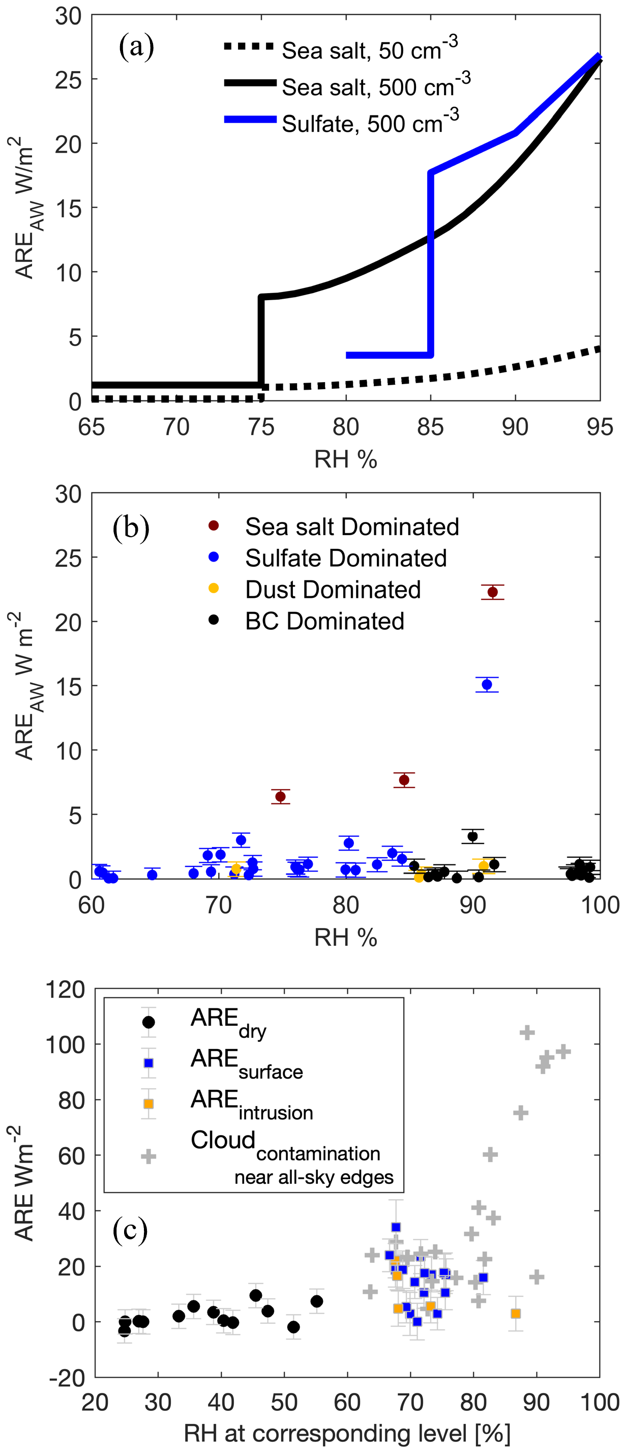
Figure 1 (a) Aerosol radiation effect (ARE_AW) of sea salt (red, black, and blue lines) and sulfate (dotted black line) as a function of RH, simulated by LBLDIS with different number density cases. (b) ARE_AW of sea-salt- (brown), sulfate- (blue), dust- (yellow), and BC-dominant (black) cases measured by the emission FTIR (NYAEM-FTS). The aerosol composition retrieval method is given in Sect. 4.3, and the methods are given by Ji et al. (2023). (c) ARE under different RH profile scenarios: ARE_dry (black) means that the entire atmosphere is in a dry state (RH <60 %), ARE_surface (blue) means that there is a layer of high humidity (RH >60 %) near the ground (<1 km), and ARE_intrusion (yellow) represents a situation with a layer of high-humidity intrusion (RH >60 %) at a high altitude (>1 km). The gray crosses indicate cloud contamination. The error bars represent 1 standard deviation of the ARE calculated over a 3 h period (10:30–13:30 UTC). Note: ARE_AW in panel (a) refers to simulations, ARE_AW in panel (b) refers to measurements by NYAEM-FTS in the AW region, and ARE in panel (c) refers to the results of measurements (BSRN) in the mid-infrared range.

Figure 1b depicts the ARE_AW measurements under varying ambient RH conditions for different dominant aerosol compositions in Ny-Ålesund based on FTIR measurements. (Cloudnet is used to determine the altitude at which the aerosol was located, and then the RH value for that altitude is obtained from ERA5.) When the dominant aerosols are sea salt and sulfate, ARE_AW from the FTIR observation also increases as RH rises. The corresponding RH of sudden enhancement of ARE_AW in sea-salt-dominated cases is about 80 %–85 %, while that in sulfate-dominated cases is around 90 %. Based on FTIR observations, the aerosol composition is primarily dominated by sea salt, with sulfate playing a secondary role. Moreover, the FTIR observations align closely with model simulations (sea salt case with a number concentration of 500 cm⁻³). Both observations and simulations show that during the early stages of aerosol wet growth (75 %< RH <80 %), the aerosol infrared radiative effect increases from approximately 1–2 to 10 W m⁻². Subsequently, as RH approaches 90 %, the ARE reaches about 20 W m⁻². Conversely, for non-hygroscopic aerosols, such as dust and black carbon, ARE_AW is about 1.45±2.00 W m⁻² and does not change with RH, which is close to previous studies (Spänkuch et al., 2000; Markowicz et al., 2003; Vogelmann et al., 2003; Lohmann et al., 2010).

BSRN measurements give the ARE in the mid-infrared range, as shown in Fig. 1c. The analysis in Fig. 1c considers the ARE in three distinct scenarios: ARE_dry, ARE_surface, and ARE_intrusion, each representing single-layer high-RH scenarios based on water vapor profiles from radiosonde (for methods, see Sect. 4.4). Overall, we observe the trend that ARE increases with rising RH. Specifically, under dry conditions (RH <60 %), the ARE remains a low value of about 2.1±3.7 W m⁻² and does not vary with RH, which is consistent with previous findings (see Fig. 1a and b). As RH increases to between 60 % and 80 %, the ARE shows a significant increase. Specifically, in the cases of ARE_surface, the mean ARE averaged between 60 % and 80 % RH is approximately 14.9±8.5 W m⁻². Moreover, in all five ARE_intrusion scenario cases, there are three cases of high water vapor intrusion, but the values of ARE do not increase with RH, and only two other cases show an enhancement of ARE at 70 % RH. It is important to note that even under very high ambient humidity conditions (RH >90 %), we still observe low ARE values, which is due to the presence of non-hygroscopic aerosols (dust or BC) from FTIR measurements. Furthermore, within high-RH conditions (RH >90 %), there are no intermediate ARE values, with transitions primarily occurring within the RH range of 70 %–80 %. This indicates that prevalent hygroscopic aerosols in Ny-Ålesund undergo a transformation from a dry to a wet state within this RH range.

Notably, we differentiate the potential radiative effect from cloud contamination. In Fig. 1c, when RH is 60 %–80 %, the infrared radiative effect from aerosol only (orange and blue dots) can be about 20 W m⁻², which is comparable with the infrared radiative effect aerosol combined with potential cloud contamination (gray dots). However, when the environment becomes more humid (RH>80 %), differentiating the radiative effect between clouds and aerosol is challenging due to the observation method. This implies that the estimation of ARE with RH less than 80 % is more reliable than that of RH>80 %.

5.2 RH temperature and sea salt AOD changes in the Arctic

To depict the humidity conditions in the Arctic, Fig. 2a presents the difference in RH between 2000–2022 and 1980–2000 in the Arctic at 900 hPa in winter (DJF). In the region around Ny-Ålesund, RH has increased significantly, showing a rise of approximately 2 %–6 % compared to pre-2000 levels. Typically, during Arctic warming, rising temperatures often lead to a decrease in RH. However, the notable increase in RH at Ny-Ålesund suggests that specific humidity is increasing more rapidly in this region compared to other parts of the Arctic. This anomaly points to unique local atmospheric conditions or processes that are enhancing moisture content more effectively than elsewhere in the Arctic.

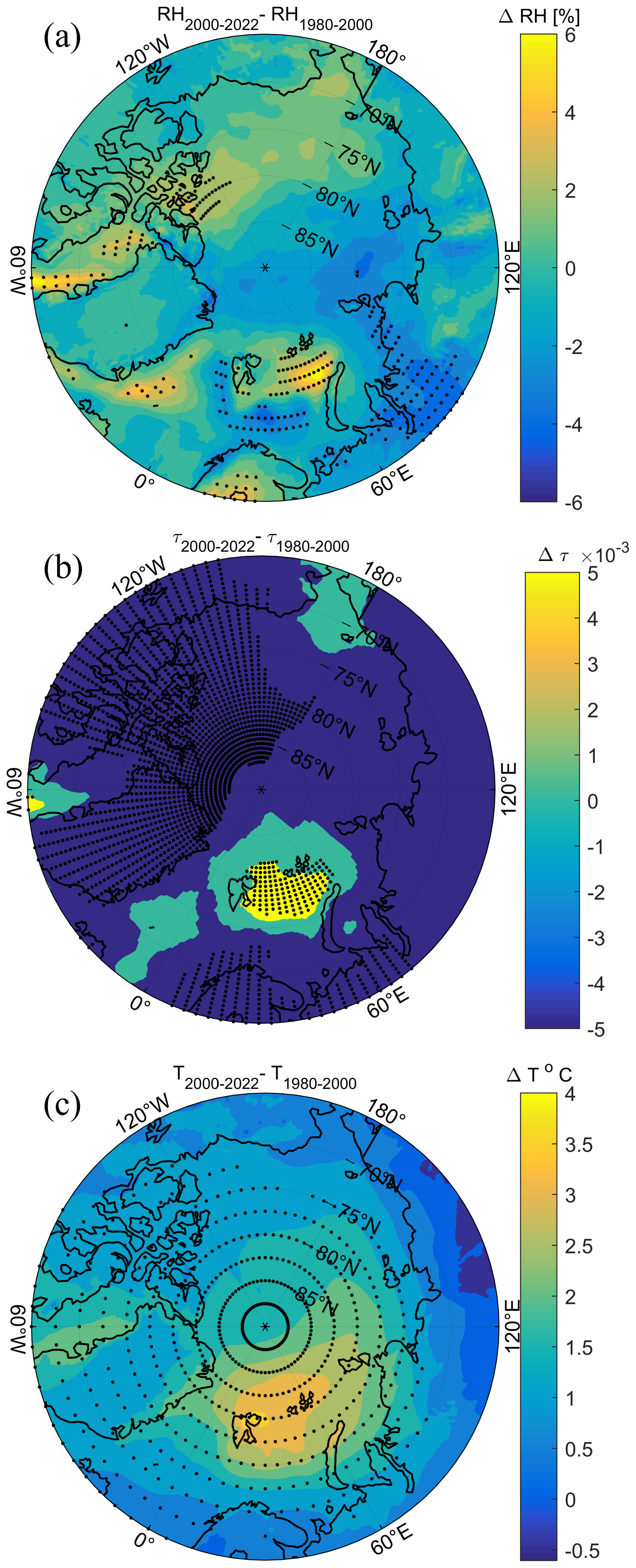
Figure 2 (a) The difference in RH between 2000–2022 and 1980–2000 in the Arctic at 900 hPa in winter (DJF), with data from ERA5 (Hersbach et al., 2023). (b) The difference in sea salt aerosol optical depth between 2000–2022 and 1980–2000, with data from MERRA-2 reanalysis data (Gelaro et al., 2017). (c) The difference in temperature between 2000–2022 and 1980–2000 in the Arctic at 900 hPa in winter (DJF), with data from ERA5 (Hersbach et al., 2023). The black dots in (a–c) mean the difference in this grid passes the significance test (95 %).

MERRA-2 reanalysis data, illustrated in Fig. 2b, indicate a general decrease in sea salt AOD across the Arctic compared to the pre-2000 period. However, there is a notable increase in sea salt AOD in Ny-Ålesund and the nearby area. The difference in sea salt AOD between 2000–2022 and 1980–2000 reveals a statistically significant positive anomaly near Ny-Ålesund of approximately $+\mathrm{0.005}.$

When combining the changes in the RH and sea salt AOD anomalies, we observe that regions with high humidity and positive sea salt AOD anomalies coincide with areas experiencing large positive temperature anomalies, as shown in Fig. 2c. Specifically, these regions exhibit temperature anomalies of around +3 °C. These findings highlight the significant role of aerosol wet growth in the Arctic. The suitable RH conditions in Ny-Ålesund have likely facilitated the wet growth of sea salt aerosols, contributing to the observed positive temperature anomalies.

6 Discussion

FTIR and BSRN observations operate on different spectral bands, with the FTIR focusing on the atmospheric window spectrum region and the BSRN covering a broader infrared spectrum. It is worth noting that the estimations of the absolute radiation value from two observation methods are not comparable because of the different spectrum range. However, if cross-validation of these methods is needed, we can roughly compare them in terms of how many times they have grown in radiation from dry to wet aerosol. Both FTIR and BSRN observations consistently indicate that within the relative humidity range of 60 %–80 %, aerosol wet growth results in an approximate 7 times increase in ARE compared to dry conditions. At high humidity (>80 %), the FTIR instrument can capture the infrared radiative enhancement by aerosol wet growth because of the small field of view (FOV =3.3 mrad). In contrast, BSRN all-sky observations, which require a completely cloud-free sky across the entire observation domain, are more susceptible to cloud contamination under high-humidity conditions. As a result, the BSRN is limited in providing precise ARE values at higher-humidity levels. This distinction highlights the strengths and limitations of each observational method under different atmospheric conditions.

Our study shows that wet aerosols have an additional warming effect. However, when the relative humidity exceeds 80 %, Cloudnet always observes some cloud signals during the period beyond the 180 min window in BSRN measurements. We cannot conclusively determine whether high values of LWD (>40 W m⁻²) are solely caused by aerosols or the result of cloud contamination (see Fig. 1). Under very humid conditions (RH >80 %), wet aerosols become activated and transform to cloud droplets. This phenomenon from the BSRN observation aligns with our hypothesis, indicating that the observed ambient RH corresponds to the deliquescence point, such as 80 % for sea salt (Peng et al., 2022). Given that the maximum ARE value for RH levels between 60 % and 80 % is approximately 36 W m⁻², values exceeding this threshold may be attributed to cloud droplets. The results of this study indicate that when an instrument is unable to differentiate between the particle sizes of aerosols and cloud droplets with sufficient accuracy, utilizing the ARE or LWD to distinguish between aerosols and clouds can be a potential method.

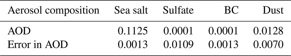
Based on the FTIR measurements and LBLDIS model simulations, RH and aerosol composition are the most important factors influencing ARE_AW. The measurement of aerosol composition, especially by remote sensing methods, is still challenging. In this study, we applied an FTIR retrieval algorithm to retrieve an aerosol composition measurement for all RH conditions, which complements the previous method in Ji et al. (2023). According to Ji et al. (2023), the larger the AOD, the stronger the aerosol composition signal and the more reliable the retrieved results. For example, in this study, in the case of a sea-salt-dominant event (cf. Fig. 1b), as shown in Table 1, the AOD of the sea salt is 0.1125±0.0013, while that of dust aerosol in this case is 0.0128±0.007. BC (0.0001±0.0013) and sulfate aerosol (0.0001±0.0109) are present during this event; however, their contribution is not the dominant factor. In other words, the error in the dominant aerosol composition in the AOD retrieval is about 1.16 %. Furthermore, as analyzed in Sect. 4.1, the error in ARE_AW measured by the FTIR is about 0.550 W m⁻², which is more accurate than that from the BSRN (about 5 W m⁻²). Therefore, the emission FTIR is a helpful instrument to do the aerosol composition and ARE measurements.

Table 1 Retrieval results (AOD and error) from an aerosol event dominated by sea salt.

Several studies have shown that Arctic water vapor content is increasing, primarily due to enhanced poleward transport from mid-latitudes via atmospheric river pathways (Sato et al., 2022; Thandlam et al., 2022; Bresson et al., 2022; Lauer et al., 2023). ERA5 reanalysis data, as presented in Fig. 2a, indicates that Ny-Ålesund has high water vapor levels during winter, providing suitable ambient RH conditions for aerosol wet growth. MERRA-2 reanalysis data further reveal a positive anomaly in sea salt AOD in the area around Ny-Ålesund after 2000 (Fig. 2b). Moreover, numerous studies have indicated that during the winter season, sea salt aerosols can dominate the Arctic aerosol composition (Huang and Jaeglé, 2017; Kirpes et al., 2018). Our results (Fig. 1b) corroborate this, demonstrating that in scenarios dominated by sea salt aerosols, the infrared radiative effect is most pronounced in Ny-Ålesund. Kirpes et al. (2018) also affirm that sea salt constitutes the principal contributor to accumulation- and coarse-mode aerosols during the Arctic winter. Heslin-Rees et al. (2020) have demonstrated that coarse-mode aerosols, primarily originating from sea spray, have exhibited an increase over the last 2 decades (1999–2016) at the Zeppelin Observatory in Svalbard. This observed trend can be attributed predominantly to alterations in air mass circulation patterns, with a higher frequency of air masses originating from the northern Atlantic region (Pernov et al., 2022).

Our measurements, yielding high ARE of hygroscopic aerosols and very low ARE of non-hygroscopic aerosols, indicate sea salt aerosols are very important for the Arctic warming in winter. MERRA-2 reanalysis data, as shown in Fig. 3, confirm our results that in Ny-Ålesund, sea salt and sulfate aerosols are significantly more dominant than other aerosol components in winter. As spring arrives, sea salt AOD begins to decline, while dust AOD gradually increases. Arctic dust aerosol primarily originates from natural sources such as desert regions, with approximately 65 % from Africa (Sahara), 22 % from Asian deserts, and 13 % from other deserts (Kok et al., 2021; Breider et al., 2014). Arctic dust aerosol concentrations peak in spring when long-range transport from Africa and Asia is most efficient (Groot Zwaaftink et al., 2016). This trend continues into summer, when sea salt levels reach their lowest point. Given that sea salt is a major component of winter aerosols, its contribution to Arctic winter warming requires further investigation in the future.

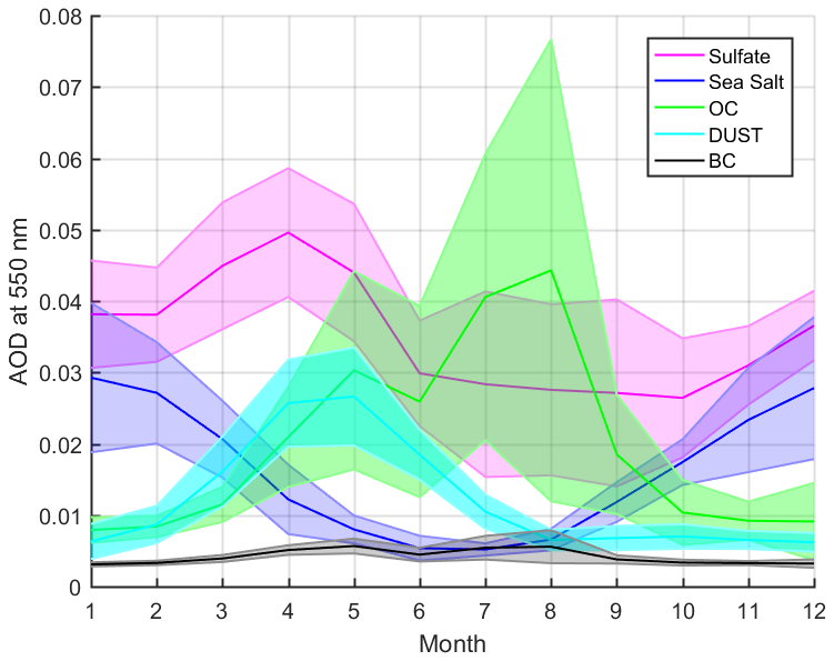
Figure 3 Seasonal variation in sulfate, sea salt, OC, dust, and BC from MERRA-2 reanalysis data averaged from 2002 to 2021 with 1 standard deviation (shaded area) in Ny-Ålesund.

Combining the changes in RH and the sea salt AOD anomaly, the region of high humidity with positive sea salt AOD anomalies overlaps the regions with large positive temperature anomalies (see Fig. 2c). Based on these findings, it is crucial to consider the warming effect of aerosols under high-humidity conditions when studying Arctic amplification. The greenhouse effect of water vapor intensifies surface warming, leading to higher humidity levels in the Arctic (Beer and Eisenman, 2022), which facilitates aerosol wet growth. Increased aerosols in a wet state further warm the Arctic atmosphere, potentially leading to more water vapor and creating a positive feedback loop in Arctic amplification. Therefore, studying the longwave radiation (LWD) contributions from both water vapor and aerosols together is essential.

Although the area of positive sea salt AOD anomalies is very limited in the Arctic, the differences in the deliquescence and efflorescence points during the aerosol wet growth process can have the potential to expand the warming effect of aerosols throughout the whole polar region. Wet aerosols can maintain their hydrated state until they either develop into cloud droplets in supersaturated conditions or revert to dry particles in drier environments, typically below the efflorescence point (Lillard et al., 2009). For instance, as shown in Fig. 4, sodium chloride (NaCl) has a deliquescence point of approximately 75 % RH and an efflorescence point of around 46 % RH (Peng et al., 2022). Consequently, NaCl remains in a wet state after activation (the dashed black line in Fig. 4) until ambient RH drops below the efflorescence point (e.g., 45 % RH). Therefore, the Ny-Ålesund region can act as a “refueling station” for the wet growth of the hygroscopic aerosols, specifically the sea salt aerosols, resulting in a warming effect. Here, these aerosols are activated, and after leaving the region, they can remain activated and travel throughout the Arctic, carrying high values of ARE as long as the ambient humidity is higher than the efflorescence point.

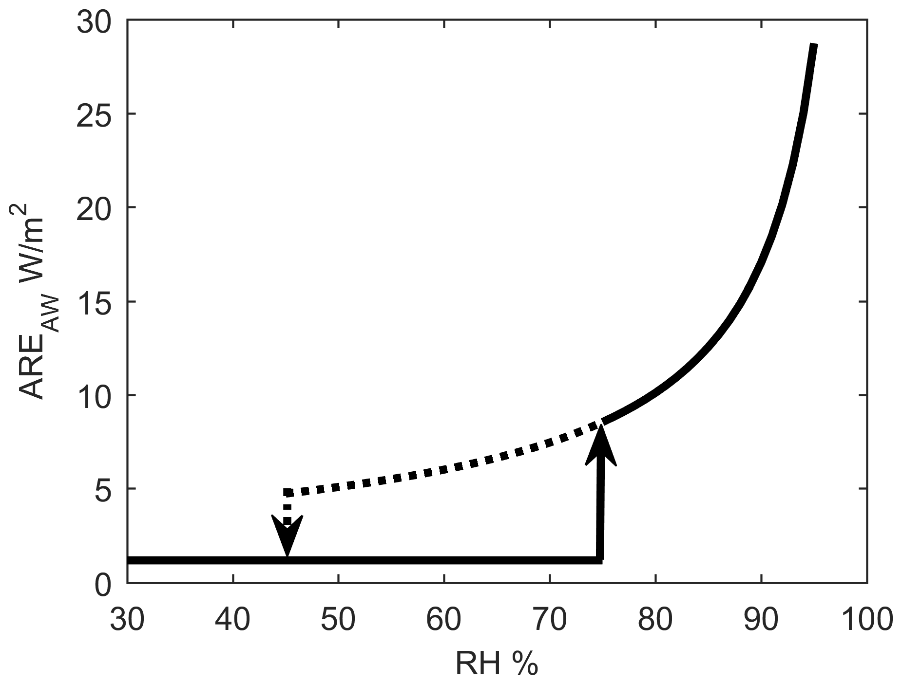
Figure 4 Graph depicting aerosol radiative effects (AREs) as a function of relative humidity (RH), accounting for the deliquescence and efflorescence points. The aerosol component illustrated is sodium chloride, with an aerosol number concentration of 500 particles per cubic centimeter. The deliquescence point is set at 75 %, and the efflorescence point is at 46 %.

7 Conclusions

In this study, based on the measurements from the FTIR, the BSRN, Cloudnet, and radiosonde, the infrared radiative effect of aerosols during the wet growth process has been investigated. Under dry conditions (RH <60 %), the ARE in the whole mid-infrared range remains about 2.1±3.7 W m⁻². As RH increases, a significant increase in ARE is observed. Between RH levels of 60 % and 80 %, the average ARE is about 14.9±8.5 W m⁻², about 7 times higher than that of dry aerosols. Moreover, in cases where the aerosol layer becomes more humid (RH >80 %), according to the FTIR measurement, the ARE can be up to 20 times higher than that in the dry state. Moreover, the prevalent hygroscopic aerosol in Ny-Ålesund from FTIR measurements is sea salt, undergoing a transformation from a dry to a wet state within the RH range of 70 %–80 %. The analysis of ERA5 data indicates that Ny-Ålesund has maintained RH levels above 80 %, which are conducive to the wet growth of aerosols. MERRA-2 reanalysis data show a positive anomaly in sea salt AOD in this area of approximately +0.005 compared to the pre-2000 period. Combining the RH and sea salt AOD, the study finds that areas with high humidity and increased sea salt AOD overlap with regions experiencing significant positive temperature anomalies. Furthermore, if aerosols are highly activated in Ny-Ålesund, they will remain activated after leaving the region as long as the ambient humidity is above the efflorescence point and will propagate throughout the Arctic with high values of ARE.

The results highlight the importance of aerosol wet growth in influencing Arctic climate. The high humidity in Ny-Ålesund and the nearby area around Svalbard likely promotes the growth of sea salt aerosols, which in turn may contribute to warming through increased longwave downward radiation. These interactions are crucial for understanding Arctic amplification. Continuous monitoring and detailed analysis of these factors are essential for predicting future changes in the Arctic environment.

Appendix A: Non-isotropic emissions correction coefficient

The relationship between the integral calculation of radiance in the AW region, II_AW, and the cosine of the zenith angle, μ, is assumed to be exponential. Figure A1 presents the relationship between II_AW and μ. The integral of the fitted function with μ could be calculated as the correction coefficient in Eq. (4) after getting the fitted function (dotted black lines), and the flux in units of W m⁻² could then be obtained. In this figure, the aerosol type is dry sea salt with a 1 µm (diameter). The method of aerosol hygroscopic growth mentioned in Sect. 4.3 is used to calculate the wet particles. The varied colors indicate the various number densities of sea salt, while the black line stands for a clear-sky scenario. Four cases from the LBLDIS simulation in four RH conditions (65 %, 75 %, 85 %, and 95 %) are provided as well. When the aerosol number density is low, between 50 and 500 cm⁻³, the ratio of II_AW(μ) to II_AW(μ=1) at various u remains relatively constant. With a sharper relationship in dry conditions and a progressive flattening with an increase in RH, this phenomenon occurs in all RH cases. Furthermore, the differences in the equations at higher relative humidity levels (75 %, 85 %, and 95 %) are not apparent, suggesting that the correction coefficient for non-isotropic aerosol scenarios may be similar under wet conditions. Additionally, such a relationship dramatically flattens as RH rises in the presence of heavy aerosol pollution, such as that present in the case of 5000 cm⁻³, and tends to be isotropic in high-RH conditions, as in the case of RH =95 %. We anticipate that under high-RH conditions, a significant number of aerosols will progressively activate and develop into a thick cloud in the atmosphere that emits isotropic radiation.

Following the simulation of sea salt, sulfate aerosol is also calculated by LBLDIS. Table A1 displays all results, including the atmosphere on a clear day. The correction coefficient for a clear atmosphere is approximately 1.08. For a clear sky, the light from atmospheric emission could be very nearly isotropic, while for aerosols, sea salt has a correction coefficient of 1.40 in a dry state and roughly 1.35 in a wet state, which is considerably different from a clear day. Although the activated RH for sulfate aerosol and sea salt is different (75 % for sea salt and 85 % for sulfate), both exhibit similar correction coefficient values when they are activated.

In conclusion, non-isotropic radiance emission from aerosols should be taken into account while doing flux calculation for a moderate-aerosol event, which frequently occurs in the Arctic. In dry conditions, aerosols have a different correction coefficient than they do in wet conditions. It is not very varied for various aerosol types.

Table A1 The correction coefficient for the atmosphere, sea salt, and sulfate at different RHs.

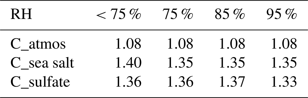
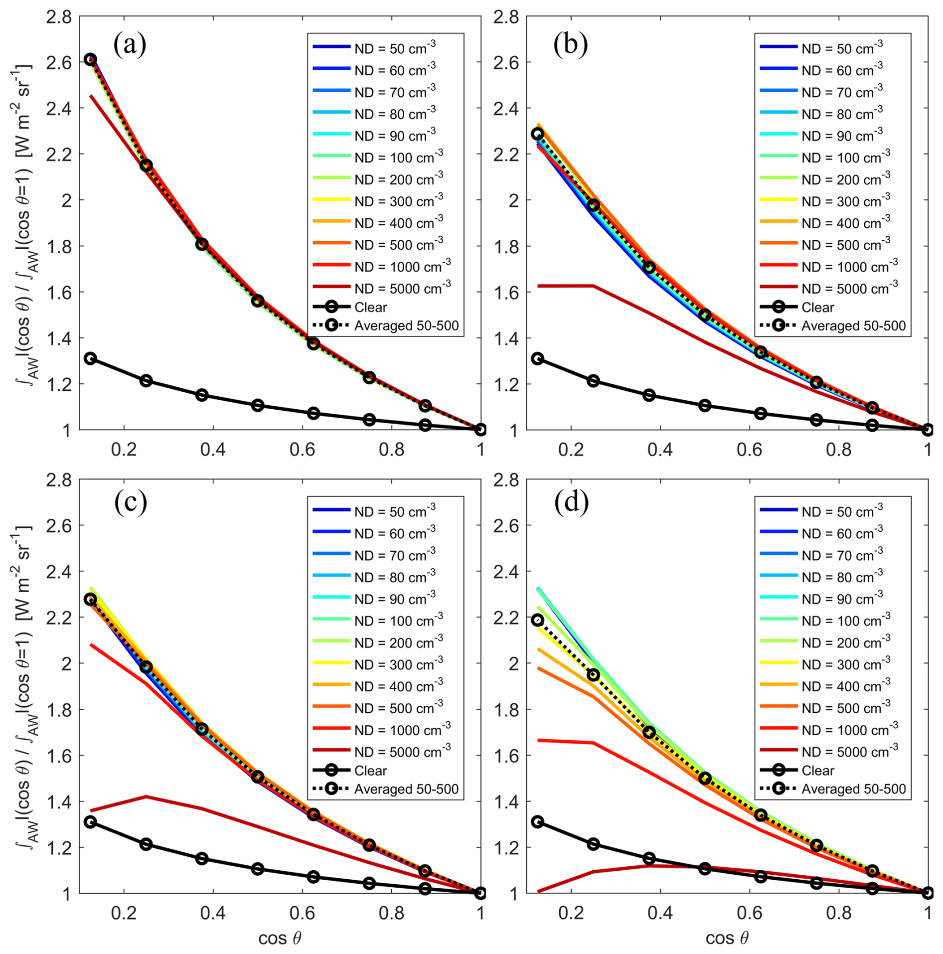
Figure A1 (a) The relationship between II_AW and μ. The varied colors indicate the various number densities of sea salt, while the black line stands for a clear-sky scenario. The dotted black lines are the averaged values from 50 to 500 cm⁻³. Four cases from the LBLDIS simulation in four RH conditions (65 % in a, 75 % in b, 85 % in c, and 95 % in d) are provided as well.

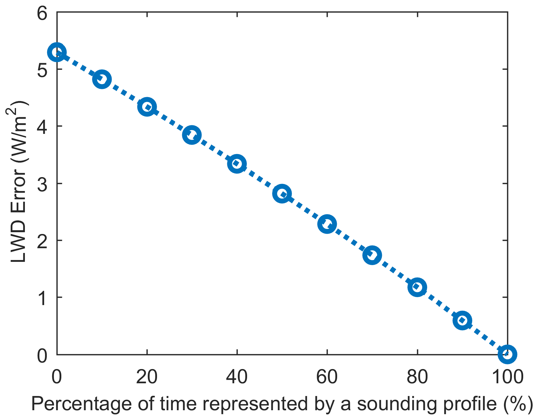
Figure A2 Errors in LWD due to uncertainty in the proportion of time that can be represented by the 90 min profile over a 3 h period, simulated using SBDART. The model simulation for longwave downward radiation (LWD) involves changing only the water vapor column content, keeping other atmospheric conditions constant. For example, assuming the profile observations (90 min) are representative of only half of the 3 h period, we consider the following scenario: the profile accurately represents the atmospheric state (0.3 g cm⁻², Pałm et al., 2010) for half of the time in Ny-Ålesund, while the other half is characterized by subpolar conditions (0.42 g cm⁻², model default). This scenario results in an LWD effect of approximately 2.8 W m⁻².