Co-variability drives the inverted-V sensitivity between liquid water path and droplet concentrations

Climatological data of the liquid water path (LWP) and droplet concentration (N_d) often reveal an inverted-V relationship, where LWP increases and then decreases as N_d increases. Our findings show that while this LWP response to an increase in N_d aligns with proposed causal mechanisms, such as entrainment evaporation feedback and precipitation suppression, the inverted-V pattern is primarily driven by the co-variability between LWP and N_d. This co-variability arises from (1) large-scale meteorology, which controls both LWP and N_d, causing them to vary in opposite directions simultaneously, and (2) microphysical processes, where an increase in LWP is typically accompanied by a decrease in N_d. Consequently, we suggest that the inverted-V sensitivity should not be used as evidence for positive radiative forcing through LWP adjustments to aerosols as it is largely explained by co-variability. We further demonstrate that the inverted-V relationship essentially reflects the climatological evolution of Stratocumulus clouds (Sc). Therefore, background anthropogenic changes in N_d should, in principle, be reflected in the redistribution of occurrences across the inverted V while maintaining its shape.

1 Introduction

Aerosol–cloud interactions are the greatest source of uncertainty in estimates of anthropogenic perturbations to the Earth's energy budget (Forster et al., 2021; Boucher et al., 2013). Increases in atmospheric aerosols change cloud droplet number concentrations (N_d), which in turn can change the cloud properties such as liquid water path (LWP) and cloud cover. These changes, known as “cloud adjustments” to aerosol perturbations (Albrecht, 1989), can lead to a significant cloud radiative forcing. However, the magnitude and even the sign of this forcing are uncertain (Bellouin et al., 2020; Forster et al., 2021). Of great interest are the LWP cloud adjustments to N_d, which have been shown to be positive, negative, or exhibit a weak variable response (Fons et al., 2023; Glassmeier et al., 2021; Gryspeerdt et al., 2019; Manshausen et al., 2023; Toll et al., 2019).

Several studies have shown consistent evidence of an inverted-V sensitivity of LWP to increases in N_d (Arola et al., 2022; Glassmeier et al., 2021; Gryspeerdt et al., 2019; Mülmenstädt et al., 2024). The inverted V emerges from joint histograms of N_d and LWP in the log–log space in which each column is normalized so that it sums to 1 (see Fig. 1a, which shows a 2D bin-averaged plot based on the joint histogram presented in Fig. S1 in the Supplement). It indicates two opposite sensitivity regimes in the relationship between LWP and N_d: positive for precipitating clouds and negative for non-precipitating clouds. The negative sensitivity, which dominates in most observed clouds, was an important line of evidence in Chap. 7 of the Intergovernmental Panel on Climate Change’s Sixth Assessment Report, supporting the conclusion of positive radiative forcing associated with decreased LWP (Forster et al., 2021).

The two sensitivity regimes align with the microphysical understanding of clouds' responses to aerosol perturbations. In precipitating clouds, an increase in aerosols leads to smaller droplets, which limit the efficiency of collision–coalescence and thus suppress precipitation (Albrecht, 1989; Koren et al., 2014; Rosenfeld, 2000). As a result, more cloud water is retained in the cloud, and LWP increases. In non-precipitating clouds, smaller droplets associated with higher aerosol levels lead to a sedimentation–entrainment feedback, suppressing droplet sedimentation and enhancing radiative cooling at the cloud tops (Ackerman et al., 2004; Bretherton et al., 2007b). Additionally, they contribute to an evaporation–entrainment feedback, where smaller droplets experience faster evaporation timescales (Wang et al., 2003; Xue and Feingold, 2006). Both processes lead to a decrease in LWP by enhancing the entrainment of dry air from the free troposphere into the cloud layer.

These physical processes explaining the observed inverted-V sensitivity offer a convincing understanding of the causal mechanisms involved. However, alternative interpretations remain possible. An increasing number of recent studies suggest that the inverted V is influenced by co-variations between LWP and N_d or satellite retrieval biases (Arola et al., 2022; Fons et al., 2023; Glassmeier et al., 2021; Kokkola et al., 2024; Mülmenstädt et al., 2024). For instance, Fons et al. (2023) developed a methodology to remove confounding influences from large-scale meteorology and showed the importance of accounting for the co-variability between cloud depth and droplet size. This is in line with George and Wood (2010), who did a comprehensive study of the Stratocumulus clouds (Sc) in the Southeast Pacific (SEP) Ocean. They showed that the influence of continental aerosols on the Sc is associated with synoptic conditions that favour a shallower marine boundary layer (MBL), which caps the cloud top heights and thus limits the LWP, resulting in a negative correlation between LWP and N_d. Their study demonstrates how meteorology could complicate the interpretation of such correlations as being due to cloud response to aerosols. Similar insights come from Mülmenstädt et al. (2024), who used global climate models (GCMs) and found that the MBL depth and N_d in the Southeast Pacific (SEP) Ocean are anticorrelated, which might explain the negative sensitivity regime of the inverted V. Nevertheless, the response of LWP to increases in N_d is consistent with physical process understanding from theory and model simulations (Ackerman et al., 2004; Albrecht, 1989; Bretherton et al., 2007b; Koren et al., 2014; Rosenfeld, 2000). Here, we address this ambiguity.

2 Methods

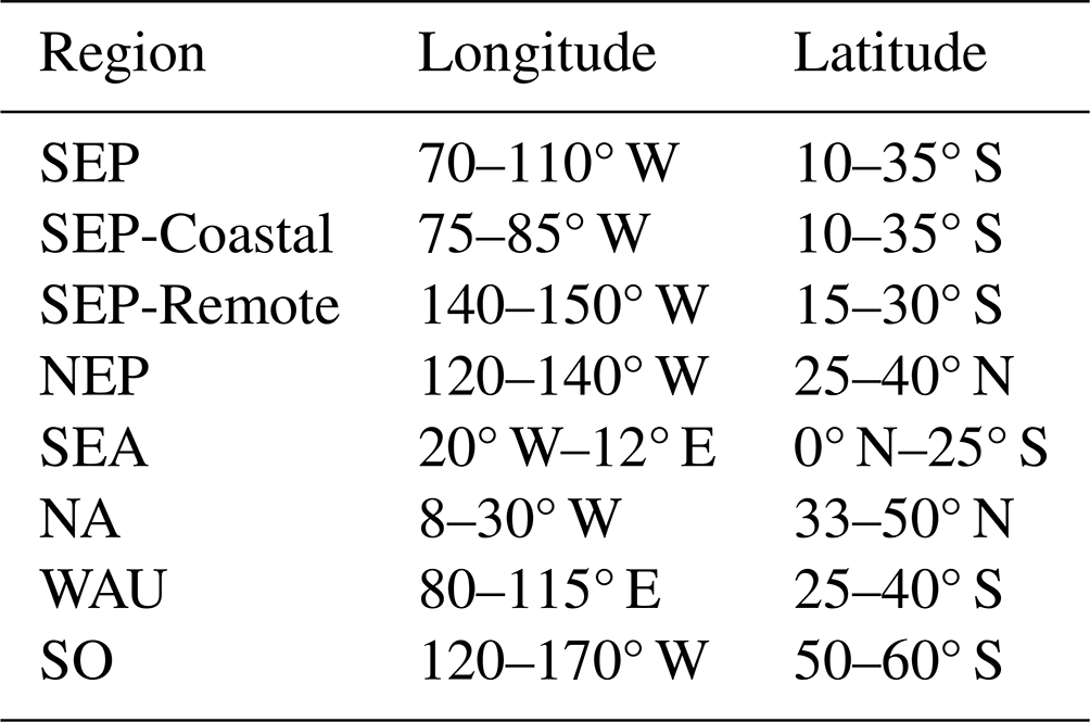
We selected the major Sc regions of the Southeast Pacific, Northeast Pacific, Northeast Atlantic, Southeast Atlantic, and western Australia (see Table 1 for region limits). We focus on marine low-level clouds in these Sc regions because they contribute significantly to the uncertainties in cloud–radiation interactions and to the differences between models and observations (Christensen et al., 2022; Gryspeerdt et al., 2022; Neubauer et al., 2014).

Table 1 Latitude and longitude boundaries of the analysed oceanic regions. SEP: Southeast Pacific, NEP: Northeast Pacific, SEA: Southeast Atlantic, NA: North Atlantic, WAU: West Australia, SO: Southern Ocean. A map showing the geographical bounds of these regions is provided in Fig. S7.

We used instantaneous satellite observations of microphysical cloud properties from the Moderate Resolution Imaging Spectroradiometer (MODIS) instrument (Platnick et al., 2017), with a nadir resolution of 1 km by 1 km. The parameters used in this study include the corrected reflectance at 0.64 µm (R), cloud cover, cloud optical thickness (τ_c), liquid water path (LWP), and cloud effective radius (r_e). N_d was calculated from r_e and τ_c following Grosvenor et al. (2018). We filter the MODIS scenes to include only single-layered liquid-phase clouds based on the MODIS cloud multi-layer flag and the MODIS cloud-phase metric. We exclude pixels with sensor angles >55° and solar zenith angles > 65° as those were shown to have retrieval-related uncertainties (Grosvenor et al., 2018). The filtered in-cloud properties were gridded into a uniform latitude and longitude grid of 1° by 1°.

We define optically thin clouds as pixels that have a τ_c≤3, as shown by O et al. (2018a) and McCoy et al. (2023). However, relying on valid τ_c retrievals alone might underestimate the optically thin cloud fraction because of failed τ_c retrievals (Cho et al., 2015). To overcome this, we follow the approach of Choudhury and Goren (2024), in which the observed relationship between R and successfully retrieved τ_c is used to classify cloudy pixels with a failed τ_c retrieval as optically thin (for more details please refer to Choudhury and Goren, 2024).

ERA5 hourly data at a uniform latitude–longitude resolution of 0.25° by 0.25° (Hersbach et al., 2020) was used for the sea surface temperature (SST) and the temperature at 800 hPa. We use these properties to calculate the marine cold-air outbreak parameter (M) (Fletcher et al., 2016; Kolstad et al., 2009), a measure of lower tropospheric stability defined as

$$\begin{array}{}\text{(1)}& \mathrm{M}={\mathit{\theta }}_{\mathrm{SST}}-{\mathit{\theta }}_{\mathrm{800}},\end{array}$$

where θ_SST and θ₈₀₀ represent the potential temperatures at the surface and 800 hPa, respectively. Note that the surface refers to the sea surface and not the near-surface layer in the atmosphere. M was found to be strongly correlated with the MBL depth (McCoy et al., 2023; Naud et al., 2018, 2020), which is the motivation for using it in our study.

The Sc regime identifications are developed by applying the supervised neural network algorithm designed in Wood and Hartmann (2006) to MODIS LWP data. The algorithm uses the power density function and power spectrum of LWP to determine whether swath sub-scenes of 256 km × 256 km fall into one of three categories: open cells, closed cells, and remaining low clouds as cellular but disorganized. Sub-scene classifications are then re-gridded onto a 1° by 1° grid (Eastman et al., 2024). The climatological occurrence of each type of regime is accumulated in each grid point, from which the red–green–blue (RGB) composites are derived. A gamma correction of 1.2 was applied to the red (closed cells) and green (open cells) composites to adjust the brightness of the image and improve its visual representation.

3 Results

Figure 1a shows the inverted-V pattern for the SEP Sc region, derived using a year of MODIS observations of LWP and N_d. The mean longitude is shown in colour and reveals a robust geographical dependence: low LWP and high N_d near the coastal regions (longitude 75–85° W, cool colours) and low N_d and high LWP in the remote oceanic areas (longitude 85–100° W, warm colours). This geographical co-variability can also be seen in the annual climatology of LWP and N_d of the SEP (Fig. 1b and c, respectively). Similar geographical co-variability is manifested in the inverted V across all other Sc regions (see Fig. S2). Throughout the paper, we selected the SEP as a representative region since this region hosts one of the most persistent Sc decks, on which many studies have focused in the past (Wood, 2012).

3.1 The negative sensitivity regime of the inverted V

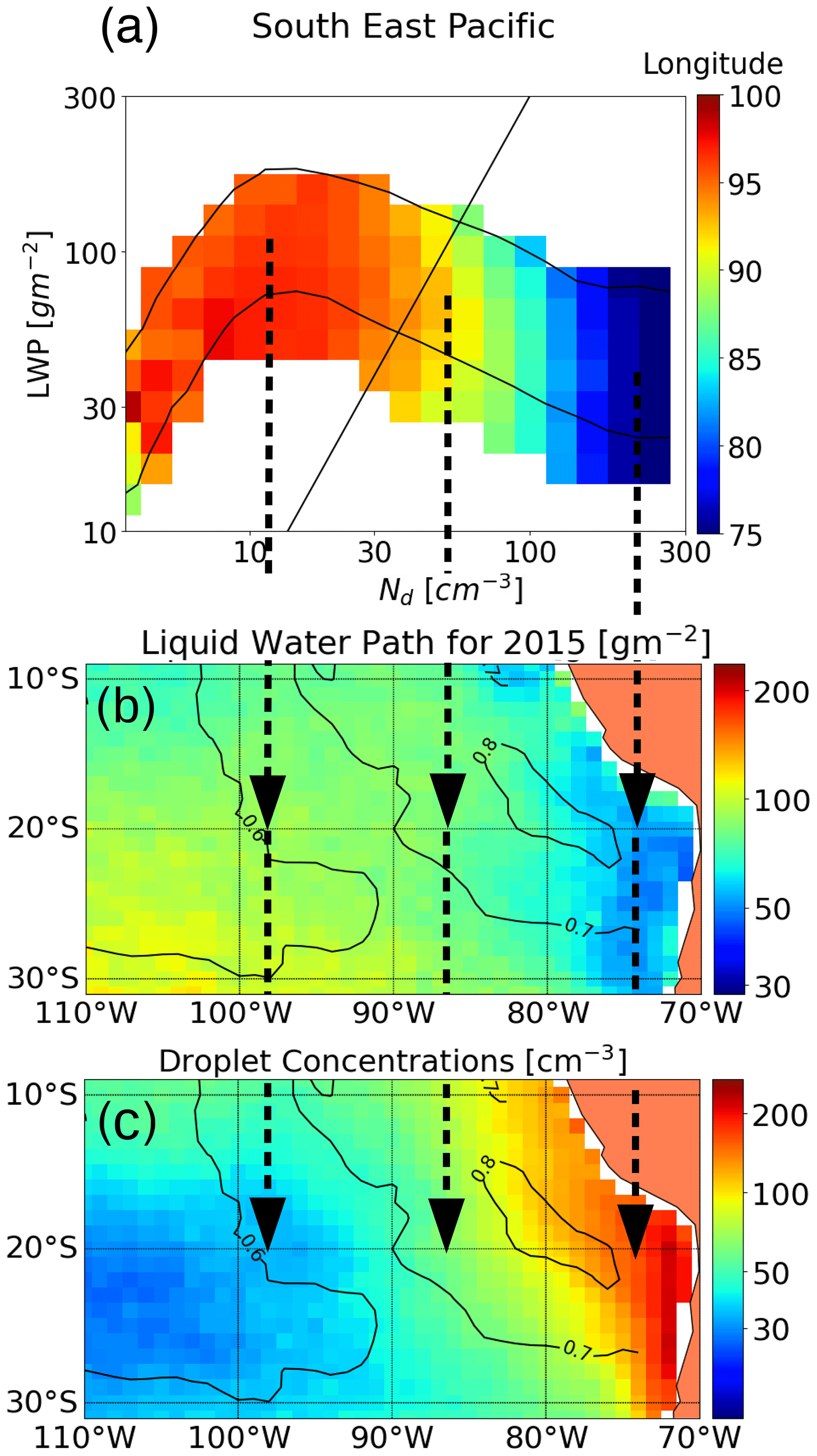
Figure 1 Inverted-V and spatial variability in LWP and N_d in the Southeast Pacific Ocean. (a) Bin-averaged longitude in N_d–LWP space. The inverted V emerges from column-normalized joint histograms of N_d and LWP (Fig. S1). The black curves bound the bins with at least 10 % of the column-normalized observations. The diagonal line represents an effective radius of 15 µm (assuming adiabatic clouds), serving as an approximate indicator of precipitation, with precipitating clouds located to the left of the line. Panels (b) and (c) show the annual mean LWP and N_d over the SEP Ocean, respectively, with contours of annual mean cloud cover. The vertical dashed arrows indicate the meridians.

The negative sensitivity regime of LWP with N_d is seen for N_d values greater than 30 cm⁻³. Observations of the Sc regions indicate that the MBL tends to be shallower near coastal regions and to deepen westward as sea surface temperature (SST) increases (Eastman et al., 2017; Sandu et al., 2010; Wood, 2012; Wyant et al., 1997). Retrieving MBL depth from observations or reanalysis is challenging and subject to uncertainties (Eastman et al., 2017). We therefore follow previous studies and use a proxy for MBL depth, M, defined as the difference between the potential temperatures at the 800 hPa level and at the sea surface (McCoy et al., 2023; Naud et al., 2018, 2020) (See Sect. 2). Figure 2a shows the mean M for each bin in the 2D joint histogram of LWP–N_d, revealing a clear gradient from right to left: low M (shallow MBL) is located on the right-hand side, while high M (deep MBL) is on the left-hand side. The MBL depth caps the cloud top height and thereby controls the vertical development of the clouds and their LWP, which is the vertically integrated cloud water. In accordance, lower (higher) LWP is associated with shallower (deeper) MBLs, as shown in Fig. 2a. Recalling Fig. 1a, shallow MBLs are prominent in the eastern SEP near the coastal regions, whereas deep MBLs are predominant in the western SEP in the remote oceanic regions. The right-to-left gradient in M therefore corresponds to an east to west gradient of MBL depth, which governs the climatological LWP. Similar results were recently shown by Mülmenstädt et al. (2024) in GCM simulations of the same region.

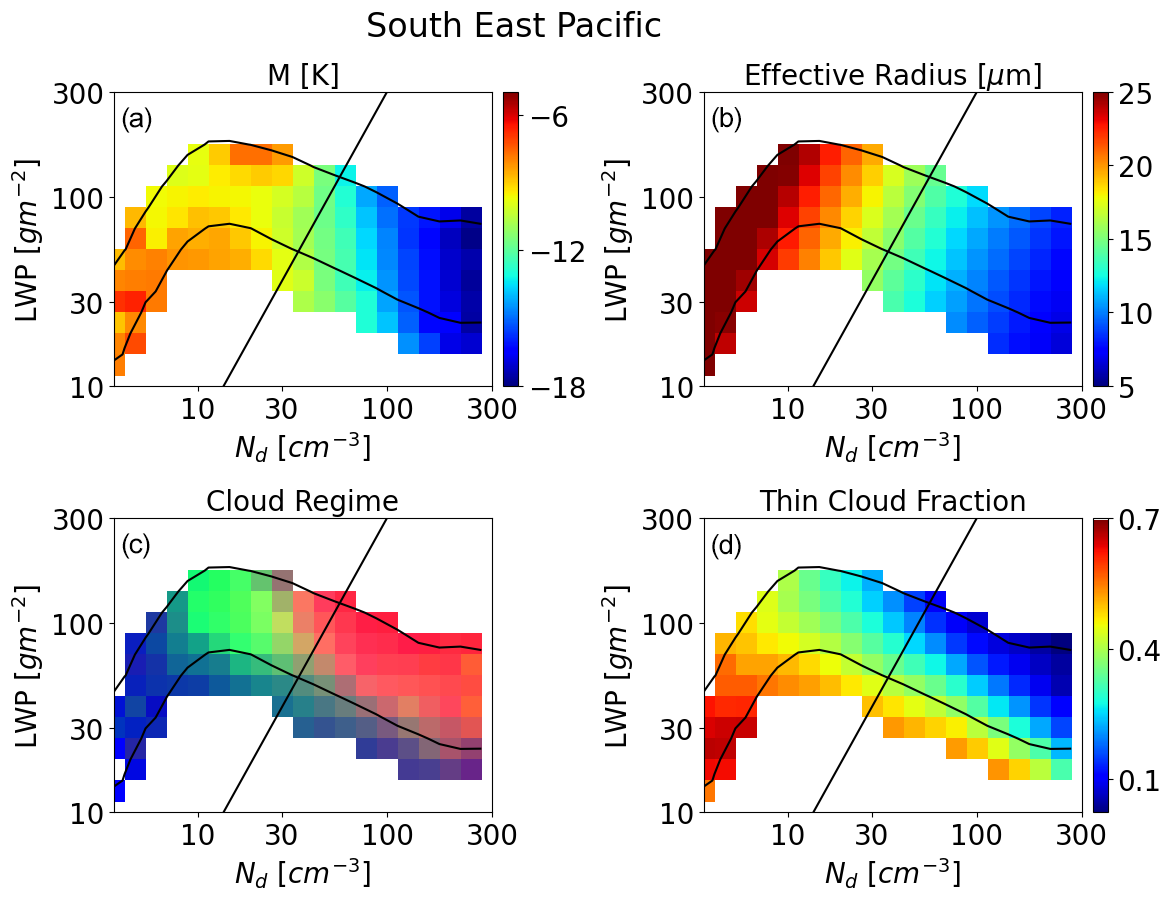
Figure 2 Bin-averaged meteorological and cloud properties in N_d–LWP space. (a) M, a proxy for MBL depth where a more negative M indicates a shallower MBL, while a less negative M indicates a deeper MBL. (b) r_e. (c) RGB composite of Sc cloud regime, where closed cells modulate the red, open cells modulate the green, and blue is modulated by other types of disorganized marine clouds. (d) Fraction of optically thin clouds (defined as cloud optical thickness smaller than 3). The black curves bound the bins with at least 10 % of the column-normalized observations. The diagonal line represents an effective radius of 15 µm (assuming adiabatic clouds), serving as an approximate indicator of precipitation, with precipitating clouds located to the left of the line.

Comparing Figs. 1a and 2a also reveals a pronounced east–west gradient in N_d. The higher N_d levels in the eastern SEP are attributed to the proximity of clouds to continental aerosol sources, i.e. South America. In the SEP, persistent southeasterly winds transport the high-N_d clouds from the coastal regions towards the remote oceanic areas downwind, where the MBL is deeper, leading to an increase in LWP (George and Wood, 2010; Sandu et al., 2010; Wood, 2012). During advection, the clouds undergo a cleansing process through collision coalescence and droplet scavenging, leading to a decrease in N_d (Christensen et al., 2020; George and Wood, 2010; Goren and Rosenfeld, 2015; Goren et al., 2019, 2022; Rosenfeld et al., 2006; Yamaguchi et al., 2015). The concurrent opposing changes in LWP and N_d can therefore also be explained by microphysical processes, which would naturally lead to a negative relationship between LWP and N_d (Gryspeerdt et al., 2022). Following this, the negative relationship between LWP and N_d should emerge in any approach that samples clouds throughout their temporal development, where clouds deepen over time and enhance the reduction in N_d via collision–coalescence process. Aerosols entraining from the free troposphere or originating from the ocean can influence the rate of decrease in N_d (Wang et al., 2010; McCoy et al., 2024), and their climatology is assumed to be included in the climatological means presented here.

3.1.1 Temporal versus spatial cloud evolution

A measure for cloud droplet size is the cloud effective radius (r_e). As clouds grow vertically, their cloud top r_e increases accordingly (Freud and Rosenfeld, 2012; Gerber, 1996; Goren et al., 2019). Figure 2b shows the mean cloud top r_e within each bin of the joint histogram, where the r_e can be seen to increase along the negative slope of the inverted V. Also note that the r_e is approximately perpendicular to the r_e=15 µm line. If LWP is increasing due to an increase in MBL depth (Fig. 2a), the increase in r_e can be attributed to the deepening of the clouds along their advection westward into the deeper MBL (Fig. S4b shows r_e versus M, where the consistent increase in r_e with a less negative M can be better seen). It is worth noting that the relationship between r_e and LWP is also expected from the functional dependence of τ_c and r_e on LWP and N_d for a homogeneous warm cloud layer (Wood, 2006).

Sandu et al. (2010) showed that the persistent winds in the Sc regions allow for a time and space equivalence assumption. This assumption was applied in Goren et al. (2022) to study the effect of aerosols on cloud cover and can be similarly employed here. Following these ideas, the climatological increase in LWP from east to west is in accordance with the simultaneous increase in cloud top r_e as if a single cloud is developing vertically over time. This time–space equivalence of cloud development was applied by Gryspeerdt et al. (2021) to study the temporal evolution of ship tracks from instantaneous satellite observations and by Rosenfeld and Lensky (1998) to examine the vertical profile of r_e in convective cloud fields from instantaneous satellite observations, which was found to be reliable based on large-eddy simulations (LESs) of Zhang et al. (2011). The above suggests that the negative sensitivity regime of the inverted V also reflects the clouds' temporal development across the Sc region, which is comparable to the clouds' longitudinal (i.e. spatial) evolution.

3.1.2 Sc regimes across the inverted V

The Sc evolution is also evident in the dominant Sc cloud regimes across the inverted V. Figure 2c shows that closed cells are most frequent where LWP is low and N_d is high (red colours), transitioning into open cells where LWP becomes larger and N_d becomes lower (green colours). This aligns with the high occurrence of closed cells near coastal regions and the increasing occurrence of open cells and other broken cloud regimes westward towards the remote oceans (Eastman et al., 2021, 2022; McCoy et al., 2023; Muhlbauer et al., 2014). Furthermore, closed cells were shown in numerous studies to exist in high-N_d conditions and to break up when N_d decreases sufficiently to initiate precipitation (Goren et al., 2019; Goren and Rosenfeld, 2014; Rosenfeld et al., 2006; Wang and Feingold, 2009), typically occurring at r_e=15 µm (Freud and Rosenfeld, 2012; Gerber, 1996; Goren et al., 2019; Rosenfeld et al., 2012). This is consistent with the r_e shown in Fig. 2b and the lines marking the r_e=15 µm in Fig. 2. It implies once again that the negative sensitivity regime of the inverted V depicts the Sc evolution across the region.

3.1.3 Local co-variability between air masses

The inverted V is also found in spatially limited areas near the coastal regions, where the full climatology of the Sc evolution across the entire region cannot be captured (Fig. 3a and b). In these areas, the inverted V emerges due to local temporal variability in air masses. Although less frequent, clean air masses with deeper MBLs (low M, Fig. 3a) can extend to the coastal regions, resulting in anomalously deeper MBLs (and thus higher LWP), while shallow MBLs (and thus lower LWP) dominate on most days. Since M also characterizes air masses originating in the polar areas (Naud et al., 2018), the polar maritime air might be relatively cleaner due to its origin and/or due to precipitation scavenging and thus have a lower N_d despite being near the coastal region.

In contrast, the inverted-V pattern, particularly its negative regime, is much less pronounced or even nonexistent in spatially limited areas of the remote oceans (see Southern Ocean example; Fig. 3c and d). This is primarily due to the lack of co-occurrence between high N_d and low LWP (Fig. S1c and d). In distant Sc regions downwind of the continents, the occurrence of scenes with low LWP and high N_d is significantly lower (Fig. S5) and the negative sensitivity of LWP with respect to N_d diminishes accordingly. This suggests that the negative sensitivity observed in the Sc regions is not necessarily a causal response of LWP to N_d but rather reflects differences in meteorological conditions. Accordingly, these findings explain the weak and positive LWP–N_d sensitivities that dominate observations in remote oceanic regions (Gryspeerdt et al., 2019).

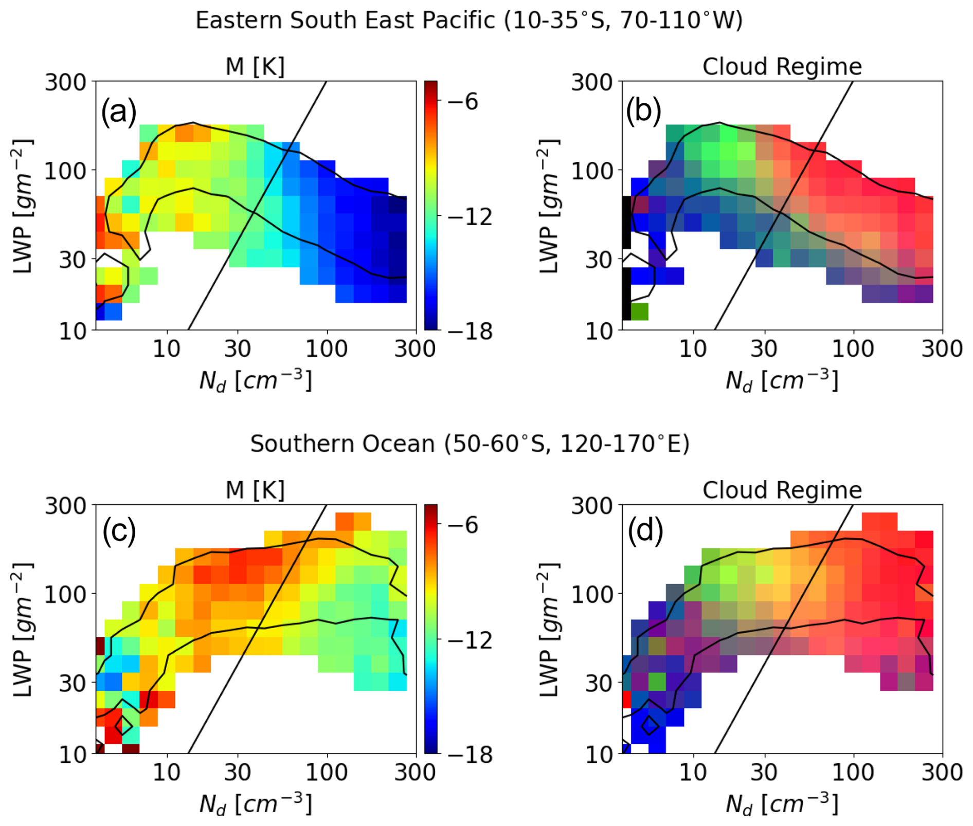
Figure 3 Mean M and cloud regimes in N_d–LWP space for a small domain near the SEP coastal region (a and b) and for the remote Southern Ocean (c and d). Refer to Table 1 for the boundaries of the regions. Panels (a) and (c) show the bin mean M, a proxy for MBL depth where a more negative M indicates a shallower MBL, while a less negative M indicates a deeper MBL. Panels (b) and (d) show RGB composites of Sc cloud regime, where closed cells modulate the red, open cells modulate the green, and blue is modulated by other types of disorganized marine clouds.

3.2 The positive sensitivity regime of the inverted V

The positive sensitivity of LWP to increases in N_d is shown in Fig. 2 to the left of the r_e=15 µm line (where r_e>15 µm). Because r_e=15 µm was shown to be associated with the onset of precipitation (Freud and Rosenfeld, 2012; Gerber, 1996; Goren et al., 2019; Rosenfeld et al., 2012), the clouds in the positive sensitivity regime are considered to be precipitating. A common explanation of the positive response of LWP with increasing N_d is precipitation suppression. Precipitation suppression is the process where an increase in aerosols leads to an increase in N_d accompanied by a decrease in droplet size, which in turn slows down collision–coalescence processes and inhibits precipitation formation (Albrecht, 1989; Koren et al., 2014), resulting in an increase in LWP.

Figure 2a shows that the clouds in the positive sensitivity regime correspond to low M (i.e. a deep MBL). Deep MBLs in the SEP are most common in the western part of the region in accordance with our analysis shown in Fig. 1 and previous studies (Eastman et al., 2017). However, despite existing in a deep MBL, it can be seen in Fig. 2d that the optically thin cloud fraction, defined as clouds having a cloud optical thickness smaller than 3 (see Sect. 2), becomes larger for a less negative M (deeper MBL) and lower N_d. This contradicts intuition so far, since one would expect deeper clouds in deeper MBLs. This contradiction is resolved when we consider the Sc regime evolution, as will be shown next.

Optically thin and ultra-clean clouds have been found to exist at the top of deep MBLs (O et al., 2018a; Wood et al., 2018) as a result of lateral diverging outflows from active updrafts in precipitating convective elements. Due to coalescence scavenging in the precipitating updrafts, the cloud top outflows have low N_d on the order of a few tens per cm³ (Choudhury and Goren, 2024; O et al., 2018a; Wood et al., 2018). The latter studies have also shown that optically thin layers are most frequent in the eastern part of the SEP in agreement with our observations (Figs. 1a and 2d). Therefore, the higher occurrence of the optically thin layers in these regions is due to the deeper MBL which allows for deeper clouds and thus precipitation, characterized by a higher occurrence of open cells and other types of disorganized convection (Goren et al., 2023; O et al., 2018b; McCoy et al., 2023; Muhlbauer et al., 2014; Possner et al., 2020).

Figure 2c shows, accordingly, the dominance of open cells at the top of the inverted V, where active updrafts exist and form well-defined open-cell structures. Open cells, as well as other disorganized shallow convection regimes, dissipate eventually, leaving behind remnants of optically thin clouds with low N_d (Choudhury and Goren, 2024; O et al., 2018a; Wood et al., 2018). This helps to explain the increase in optically thin clouds towards lower N_d and lower LWP, suggesting that the positive LWP–N_d sensitivity regime is in fact a continuation of the Sc regime evolution, decaying after the precipitating cores become inactive. Such clouds are in their dissipation stage, not in their developing stage, and therefore the precipitation suppression mechanism cannot be applied to them. It should be noted that the inverted V also emerges when restricting the scenes to cloud cover greater than 80 % (see Fig. S6), thereby reassuring that the sensitivities are not due to cloud microphysical retrieval biases in the broken cloud regimes (Cho et al., 2015; Painemal and Zuidema, 2011).

3.3 Synoptic co-variability between LWP and N_d

Sc typically form near the coasts and undergo a cleansing process as they are advected westward into the remote oceans. We therefore divide the data into days with high and low N_d at the coastal regions (defined as N_d≥100 cm⁻³ and N_d<100 cm⁻³, respectively, in longitudes <85° W), assuming that near the coasts the initial N_d of the clouds is determined, as shown by, for example, Goren and Rosenfeld (2015). Given that synoptics vary slowly in the Sc regions (George et al., 2013; Goren and Rosenfeld, 2012, 2015; Sandu et al., 2010), we can assume that the clouds observed downwind of the coastal regions are a result of the conditions that were observed upwind, i.e. near the coastal regions (Christensen et al., 2020; Goren et al., 2019; Gryspeerdt et al., 2022).

Figure 4a shows the difference in occurrence between the joint histograms of high- and low-N_d days. It can be seen that high-N_d days favour low LWP across the entire inverted-V range (blue) and vice versa (red). This demonstrates the role of the synoptic scale on the co-variability between LWP and N_d, as was also shown by George and Wood (2010) and Mülmenstädt et al. (2024). George and Wood (2010) showed that for high-N_d days, this co-variability in the SEP is a result of continental air masses that are synoptically associated with shallower MBL, which limit the clouds' vertical development and thus their LWP. This emphasizes that caution must be taken when interpreting correlations as if they are causally driven by aerosol–cloud interactions.

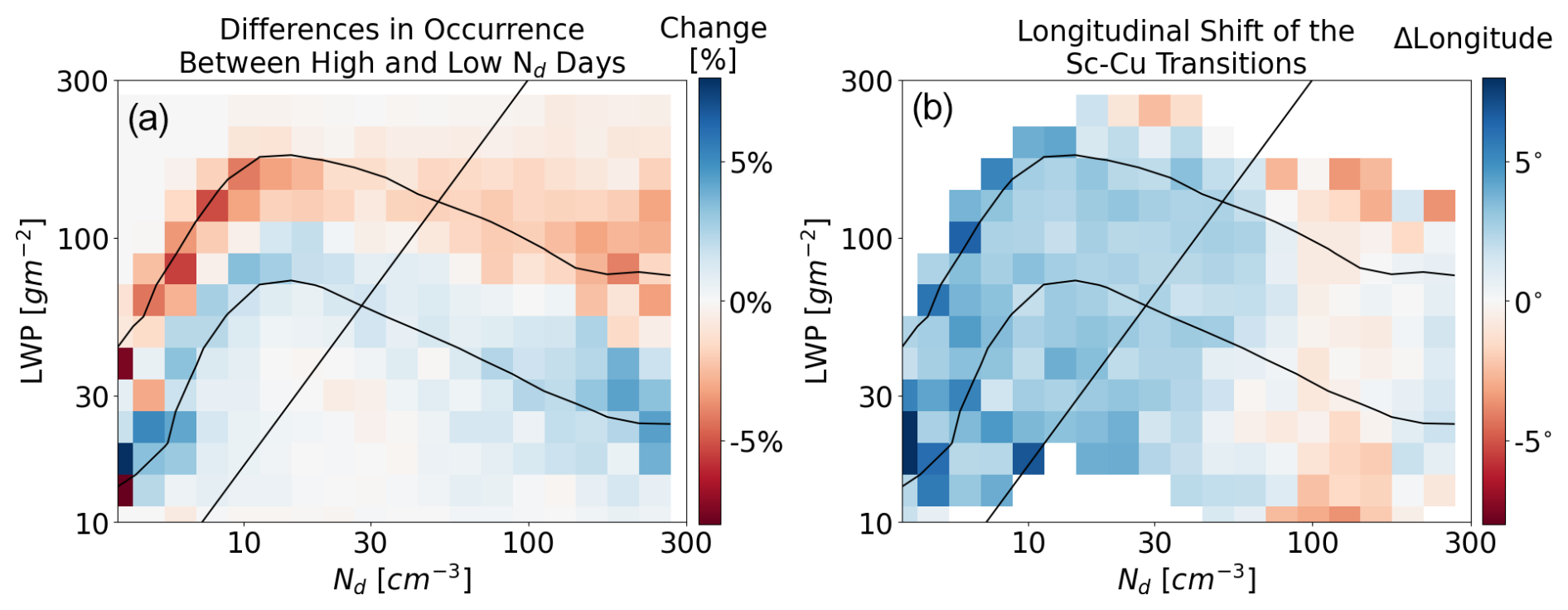
Figure 4 The effect of N_d levels at the origin of the Sc region on the inverted-V climatology in the SEP. (a) The difference in the occurrence between days with N_d≥100 cm⁻³ and days with N_d<100 cm⁻³ near the coastal region (longitude <85° W). The percentages represent the change in the normalized occurrence with respect to each column in the joint histogram, showing that the entire inverted-V shifts lower on days with high N_d near the coastal region. (b) The mean change in longitude (in colour) in each bin of the joint histogram between days with N_d≥100 cm⁻³ and days with N_d<100 cm⁻³ near the coastal region (longitude <85° W). The difference in both figures is calculated as high-N_d minus low-N_d days.

Glassmeier et al. (2021) used an ensemble of LES simulations to show that the negative sensitivity regime of the inverted V characterizes a steady state. The steady state is defined as a balance between evaporation at the cloud top, which acts to lower LWP, and the buildup of cloud water due to radiative cooling, which acts to increase LWP, with both being controlled by N_d. The downward (upward) shift of the inverted V when N_d is higher (lower) as shown in Fig. 4a might therefore be related to the steady-state hypothesis. In that sense, the steady state affects the inverted V as a whole and does not necessarily shape it. Since Glassmeier et al. (2021) sampled clouds at different stages of development (i.e. across the cloud climatology), the co-variability between LWP and N_d is an inherent characteristic that arises from the temporal development of clouds and is therefore expected.

3.4 Climatological LWP adjustments

Figure 4b shows the difference in bin-averaged longitude between high- and low-N_d days, sampled in the coastal regions. It shows that the longitude at which r_e=15 µm (where transitions from closed to open cells typically occur) shifts westward by up to 4°. This means that on days of high N_d near the coastal regions, the Sc evolution is extended further west. This is expected since such days have lower LWP (Fig. 4a), requiring the clouds to propagate further downwind into deeper MBL to gain LWP and to increase their r_e (Goren et al., 2019). This supports Gryspeerdt et al. (2022), who showed that the LWP response to N_d should be evaluated with respect to prior conditions.

Goren et al. (2019) used realistic Lagrangian LES to show that an increase in initial N_d in a given meteorological scenario delays precipitation formation and thus delays the closed-cell breakup downwind, in agreement with our results. The delayed breakup was shown to allow for the closed cells to deepen the MBL, which did not happen in the case of earlier precipitation and breakup. The role of N_d in deepening the MBL was shown in other studies (Bretherton et al., 2007a; Eastman et al., 2017) and was attributed to enhanced turbulence at cloud top due to stronger radiative cooling leading to greater entrainment (Bretherton et al., 2007a; Feingold et al., 1999). Following this, for the given climatological co-variability between LWP and N_d, an increase in background N_d (e.g. due to anthropogenic activity) would lead to an increase in LWP because clouds deepens and gain higher LWP (Goren et al., 2019). Disentangling the change in the climatological LWP due to anthropogenic N_d is challenging from observations alone, as one needs to assume a counterfactual scenario with the exact co-variability between meteorology and aerosols (Goren et al., 2022). Because N_d influences LWP through Sc regime evolution, as shown here, separating adjustments in LWP and cloud fraction is challenging due to their close interconnection.

4 Conclusions

The inverted-V sensitivity of LWP to N_d, observed in numerous studies and often interpreted causally, is shown here to reflect the Sc regime evolution from overcast closed cells to open cells and subsequently to cumulus clouds and their ultimate dissipation. Studies that sample Sc at different stages of development, i.e. across their climatology, are therefore expected to populate the LWP–N_d joint histograms in an inverted-V-shaped pattern (Arola et al., 2022; Dipu et al., 2022; Glassmeier et al., 2021; Gryspeerdt et al., 2019; Mülmenstädt et al., 2024; Possner et al., 2020).

The inverted V is separated into two regimes of negative and positive LWP–N_d sensitivities. The negative sensitivity regime arises from the co-variability between N_d and LWP. This co-variability is from two main components: (1) concurrent microphysical changes, where an increase in LWP is accompanied by a decrease in N_d, and (2) large-scale meteorology controlling the MBL depth and N_d, which vary in opposite directions simultaneously. The positive sensitivity regime reflects the dissipating stage of actively precipitating clouds, characterized by optically thin, ultra-clean cloud layers dominating the scenes (e.g. Wood et al., 2018).

Our results indicate that neither the negative nor the positive LWP–N_d sensitivities that emerge in the inverted V can be solely explained by causal effects of N_d on LWP. Those causal effects are typically referred to as entrainment evaporation feedback for the negative sensitivities (Ackerman et al., 2004; Bretherton et al., 2007b) and precipitation suppression for the positive sensitivities (Albrecht, 1989; Koren et al., 2014). Our results do not argue against the role of these physical mechanisms in the LWP response to N_d. Rather, our results demonstrate that even when a physical mechanism aligns well with observational correlations, care must be taken when interpreting these correlations as a means of inferring causality for aerosol–cloud interactions. Therefore, we suggest that the inverted-V LWP–N_d sensitivity should not be used as a line of evidence for positive radiative forcing through LWP responses to aerosols, as it is largely explained by co-variability.

The inverted V implies that the climatology of the LWP–N_d co-variability has a plausible range in each geographical location. A significant increase in N_d, such as from ship emissions (Goren and Rosenfeld, 2012; Manshausen et al., 2022, 2023; Toll et al., 2019) in areas where the background climatology of N_d is lower, creates an instantaneous increase in N_d that is detached from the plausible LWP–N_d co-variability. Such N_d perturbations reflect the causal LWP response. We therefore suggest distinguishing between the causal LWP response to N_d and the climatological response to N_d. The former is relevant for studying LWP adjustments associated with marine cloud brightening, where aerosols are injected to increase the clouds' reflectivity (Feingold et al., 2024), while the latter addresses changes in background anthropogenic N_d levels on the Sc evolution (assuming similar meteorological conditions), i.e. the effective radiative forcing from aerosol–cloud interactions (Bellouin et al., 2020).