Too cold, too saturated? Evaluating climate models at the gateway to the Arctic

The Arctic wintertime energy and moisture budgets are largely controlled by the advection of warm, moist air masses from lower latitudes; the cooling and drying of these air masses inside the Arctic; and the export of cold, dry air masses. Climate models have substantial difficulties in representing key processes in these air-mass transformations, including turbulence under stable stratification and mixed-phase cloud processes. Here, we use radiosonde profiles of temperature and moisture and surface radiation observations from Ny-Ålesund, Svalbard (1993–2014), to assess the properties of air masses being imported into and exported from the central Arctic in CMIP6 climate models. In the free troposphere, models tend to be cold-biased, especially for the coldest temperatures, and relative humidity in most models is closer to saturation with respect to ice than what is observed. In the analysed models, supersaturation with respect to ice tends to be better represented with two-moment microphysics. The overall distribution of column-integrated precipitable water in models matches well with observations. Cold and dry biases are stronger in air masses being exported from the Arctic than those entering the Arctic. This suggests that the previously reported cold bias in the Arctic in CMIP6 models is probably due to errors in local thermodynamic processes.

1 Introduction

The Arctic radiates more energy to space than it receives from the sun, and the resulting energy deficit is compensated for by heat convergence in the atmosphere and ocean, especially in winter (Mayer et al., 2019). The atmospheric energy and moisture convergence largely occurs through the exchange of air masses between the Arctic and lower latitudes (Pithan et al., 2018). Warm, moist air masses are advected polewards, where they cool and dry (Wexler, 1936; Curry, 1983; Ali and Pithan, 2020), whereas cold, dry air masses leave the Arctic and pick up heat and moisture over the open ocean in marine cold-air outbreaks (Papritz and Sodemann, 2018).

Arctic air-mass transformations are driven by and connected to the Arctic surface energy budget by thermodynamic processes in clouds and boundary layers. It is challenging to represent these processes in climate models, and earlier generations of climate models have substantial biases in their representation of Arctic climate, including the vertical temperature structure (Svensson and Karlsson, 2011; Medeiros et al., 2011; Pithan et al., 2014). Some of these biases, such as a pronounced cold bias over the central Arctic Ocean in winter, persist in CMIP6 models (Davy and Outten, 2020). The convergence of heat and moisture in the Arctic atmosphere depends on the amount of air exchanged between the Arctic and lower latitudes, which is controlled by the large-scale circulation (Woods et al., 2013; Graversen and Burtu, 2016), and on the properties, especially the heat and moisture content, of the transported air.

The particular vertical temperature structure of the Arctic atmosphere, with frequent stable stratification, is mainly due to atmospheric heat advection from the south and diabatic cooling of the surface, and it is an important condition for Arctic amplification of climate change (Manabe and Wetherald, 1975; Pithan and Mauritsen, 2014; Boeke et al., 2021).

Clouds play an important role in Arctic air-mass transformations and in the Arctic surface energy budget (Curry, 1983; Karlsson and Svensson, 2011; Cronin and Tziperman, 2015). Throughout most of the year, the warming longwave radiative effect of clouds dominates over the cooling shortwave radiative effect in the Arctic; i.e. clouds have a net warming effect on the surface (Intrieri et al., 2002). Clouds increase the emissivity of the atmosphere and can thereby increase atmospheric radiative cooling and precipitation formation (Pithan and Jung, 2021; Bonan et al., 2024).

In general, clouds form when an air parcel is (super)saturated with water vapour, i.e. when it contains more water vapour than it can sustain in a vapourized form, such that the excess water vapour condenses into cloud droplets or freezes. Because the moisture content of the atmosphere fluctuates at relatively small horizontal scales (Quaas, 2012), cloud formation can occur on much smaller scales than resolved by climate models with grid spacings of tens of kilometres and, hence, needs to be parameterized in such models.

Accurate representation of cloud phase is difficult in climate models but can have an important impact on cloud feedbacks and, thus, future climate change (Cesana et al., 2022; Tan et al., 2022). At the same temperature and pressure, the saturation vapour pressure over a liquid-water surface is higher than that over an ice surface. Air can thus be supersaturated with respect to ice but still subsaturated with respect to liquid water. In this regime, water droplets can quickly evaporate, while ice crystals grow through deposition of water molecules from the gas phase (Wegener, 1911; Bergeron, 1928; Findeisen, 1938; Storelvmo and Tan, 2015).

In real-world mixed-phase clouds, supercooled liquid water can be concentrated in thin (few tens of metres) layers near the cloud top (Verlinde et al., 2007), whereas models usually assume all condensate to be homogeneously distributed within the cloudy part of a grid box. At the same time, climate models differ in the degree of complexity used to represent mixed-phase cloud microphysics, and the respective roles of the resolution and realism of microphysical process representations for model biases are unclear.

Observational records of Arctic climate are scarce, and existing climate model evaluations largely focus on surface fields and large-scale climatological means (Davy and Outten, 2020) or remain qualitative in comparing model output to shorter field campaigns (Pithan et al., 2014; Linke et al., 2023). In this paper, we evaluate the properties of air masses exchanged between the Arctic and lower latitudes in CMIP6 models using radiosonde and surface radiation observations from Ny-Ålesund, Svalbard (Maturilli et al., 2015; Maturilli and Kayser, 2017a), which is located within the major pathway for moist intrusions entering the Arctic in winter (Woods and Caballero, 2016). We stratify observations and sub-daily model outputs by wind direction to assess poleward-moving and equatorward-moving air masses separately and to investigate the distribution of relative humidity.

We test the effect of horizontal resolution vs. parameterization complexity on the representation of supersaturation with respect to ice using output from a kilometre-scale global model and a sensitivity experiment of prescribed (one-moment microphysics) vs. prognostic (two-moment microphysics) ice number concentrations.

2 Data and methods

2.1 Observations

We use wintertime (December to March) meteorological upper-air observations by radiosondes from Ny-Ålesund, Svalbard, manually launched by the Alfred Wegener Institute since 1993. During the 3 decades since, different types of radiosondes have been used for the soundings, potentially introducing instrument-related inhomogeneities into the data record. We therefore rely on the homogenized radiosonde dataset for Ny-Ålesund (Maturilli and Kayser, 2016, 2017b; Maturilli and Dünschede, 2023), which corrects known biases of each radiosonde type (Maturilli and Kayser, 2017a). The sounding data are interpolated to the vertical resolution of the CMIP6 model output (the plev27 levels as defined in Juckes et al., 2020; see their Table 4). For comparison with CMIP6 models, we use the period of overlap with the historical runs, i.e. 1993–2014. To identify cloudy and clear-sky conditions, we furthermore use longwave radiation measurements from Ny-Ålesund (Maturilli et al., 2014; Maturilli, 2020) that are part of the Baseline Surface Radiation Network (BSRN) (Driemel et al., 2018).

2.2 Reanalysis

We use data from the ERA5 reanalysis (Hersbach et al., 2020; Graham et al., 2019) to place our findings into a large-scale context. The ERA5 reanalysis uses a fixed version of the ECMWF weather prediction model and data assimilation scheme to derive an observationally constrained estimate of the atmospheric state. In situ observations to constrain the model are scarce over the Arctic Ocean. Satellite observations are more abundant but are often rejected by the assimilation scheme (Lawrence et al., 2019). As the underlying observational data sources change over time, the reanalysis does not constitute a homogeneous record for estimating long-term trends. For example, the radiosonde measurements in Ny-Ålesund have been assimilated into the reanalysis, but no corresponding measurements exist before 1993. In this paper, we primarily use ERA5 to confirm that changes seen in the local observations on interannual to decadal timescales are representative of developments over the central Arctic Ocean.

2.3 CMIP6 models

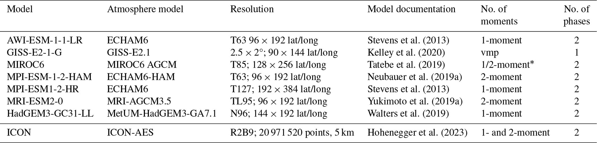
We use data for the years 1993–2014 from the first ensemble member of the historical run of the models shown in Table 1 for the CMIP6 DECK experiments (Eyring et al., 2016). Most models are in the middle range or lower range of the CMIP6 model resolution, but MPI-ESM-HR is a relatively high-resolution model. All analysed models allow for supersaturation with respect to ice in the sense that saturation with respect to ice is not a hard-coded humidity limit in the models' cloud schemes. In practice, the degree of possible supersaturation will strongly depend on the speed of the removal of water vapour through depositional growth of ice crystals. All models except GISS-E2-1-G have separate prognostic variables for liquid and frozen condensate. There is a mix of one-moment microphysics schemes with fixed or diagnostic number concentrations of cloud particles and two-moment schemes with prognostic particle number concentrations.

Stevens et al. (2013)Kelley et al. (2020)Tatebe et al. (2019)Neubauer et al. (2019a)Stevens et al. (2013)Yukimoto et al. (2019a)Walters et al. (2019)Hohenegger et al. (2023)

Table 1 Evaluated climate models and their representation of mixed-phase microphysics. “No. of phases” refers to the number of condensate phases represented by prognostic variables. ^*MIROC6 uses a two-moment scheme for warm microphysics but also a diagnostic ice number concentration. GISS uses a virtual mixed-phase scheme (vmp) to represent the effect of mixed-phase clouds within one prognostic variable for cloud condensate.

To stratify the data based on large-scale flow conditions, we use 6-hourly atmospheric profiles on pressure levels, which substantially limits our model selection. Unless described otherwise, we use data from the model grid point that is closest to Ny-Ålesund.

In climate models that use the same number of grid points in each latitude circle, the zonal grid spacing in the Arctic is much smaller than at lower latitudes. Nevertheless, the grid spacing in all models analysed here is too coarse to resolve the major topography of Svalbard (Fig. 1), which reaches up to 1500 m. MPI-ESM-HR and GISS-E2-1-G have topographies that are at least twice as high as those of other models. In all models, but especially those with less resolved topography, the mountains stretch too far in the zonal direction, which is probably a result of smoothing the topographies for spectral models. While sub-grid parameterizations attempt to represent the effect of unresolved topography on the large-scale flow, the handover between resolved and unresolved processes is far from perfect and, at best, reproduces the effects on the momentum budget (Sandu et al., 2019). Other orography-related effects such as precipitation or Foehn warming through downslope winds (Shestakova et al., 2022) can, at best, be crudely represented in the CMIP6 models given their coarse representation of orography. In this paper, we focus on the representation of the thermodynamic properties of air masses exchanged between the Arctic and lower latitudes at larger scales rather than the local topographic effects, but the possibility that observations are affected by orography that is not adequately represented in the models must be kept in mind.

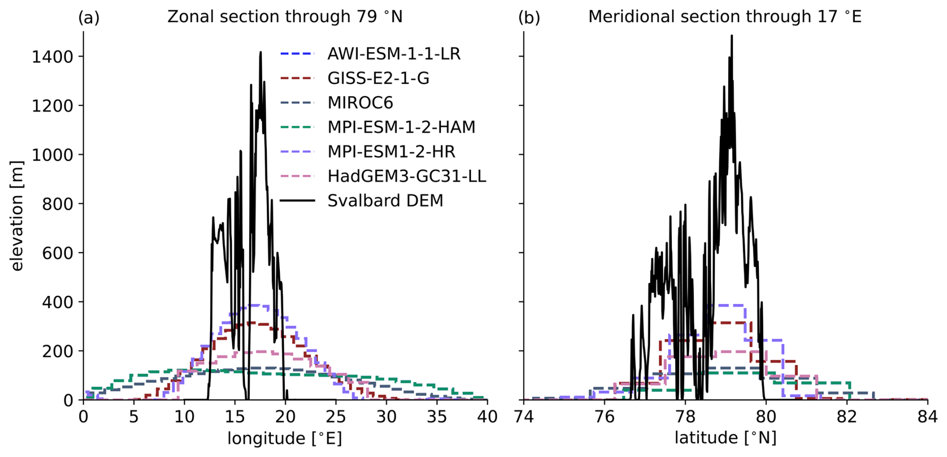
Figure 1 Zonal and meridional cross-sections through the topography of Svalbard. AWI-ESM-1-1-LR and MPI-ESM-HAM use identical grids and topographies; hence, the two lines exactly overlay each other on this plot. Svalbard DEM refers to the digital elevation model by Norwegian Polar Institute (2014).

2.4 Global storm-resolving (kilometre-scale) simulations with ICON

For some sensitivity analyses in Sect. 2b, we also consider two simulations with the storm-resolving model ICON-Sapphire (Hohenegger et al., 2023) that apply a global quasi-uniform horizontal grid spacing of 5 km. The two simulations differ only in the applied representation of microphysical processes: in one simulation, a one-moment scheme predicts the specific mass of five hydrometeor categories (cloud water, rain, cloud ice, snow, graupel; Baldauf et al., 2011), and, in the other simulation, a two-moment scheme predicts both the specific number and the specific mass of six hydrometeor categories (cloud water, rain, cloud ice, snow, graupel, hail; Seifert and Beheng, 2006). Both schemes allow for excess water vapour with respect to ice saturation, i.e. supersaturation with respect to ice. The single-moment scheme calculates a diagnostic number of ice particles which depends only on temperature. It does not allow for homogeneous nucleation of ice particles from water vapour without any nuclei but takes into account the tendencies of cloud ice specific mass due to homogeneous freezing of cloud droplets and a simple heterogeneous nucleation rate. The two-moment scheme employs a prognostic treatment of the number of ice particles and takes into account heterogeneous nucleation of ice particles (after Hande et al., 2015, including both immersion freezing and deposition nucleation), homogeneous freezing of cloud particles (after Jeffery and Austin, 1997), homogeneous nucleation of ice particles (after Kärcher et al., 2006), and Hallett–Mossop ice multiplication (after Beheng, 1982).

In addition to the parameterization of microphysics, radiation and turbulence are also parameterized but no shallow- or deep-convective parameterization is applied. The simulation setup closely follows the DYAMOND protocol (DYnamics of the Atmospheric general circulation Modeled On Non-hydrostatic Domains; Stevens et al., 2019). The model time step is 40 s, and the vertical grid consists of 110 hybrid sigma height levels with a grid spacing of 400 m in the free troposphere, which gradually decreases towards the surface and increases toward the model top. Due to their high computational cost, a simulation period of 10 d is covered by both simulations, starting on 1 February 2020.

The analysis shown in this study is restricted to the last 5 d to allow for 5 d of spinup. This is a short period for studying climatological effects, but it is long compared to the many case studies used to study the impact of microphysics on regional storm-resolving, or finer-scale, simulations. The simulations are described in detail by Naumann et al. (2024), who show that, for aggregated global statistics, differences between the two simulations are typically larger than the day-to-day variability, and, hence, the short simulation period is sufficient to identify the systematic effects of changing the representation of microphysical processes. For our analysis, the difference between the ICON one-moment and two-moment schemes that occurs in the 5 d run is robust, even for 1 d averages (Fig. S1 in the Supplement).

2.5 Separating southwesterly and northerly flows

Throughout this paper, we stratify observations and model output based on the large-scale flow. To this end, we average the observed wind speeds between 650 and 775 hPa, i.e. well above the orography that constrains the local flow near Ny-Ålesund (Maturilli and Kayser, 2017a; Schön et al., 2022). In CMIP6 models, we use wind speeds at the 700 hPa level. When this wind speed has both a westerly and southerly component, we classify the air mass as originating from the southwest, i.e. from the open ocean. When the wind speed has a northerly component, we classify the air as coming from the north, i.e. the largely sea-ice-covered Arctic Ocean, regardless of the zonal component of the flow. Differences between northeasterly and northwesterly advection (not shown) are small compared to those between northerly and southerly flows. Here, we do not show results for air masses coming from the southeast, i.e. the Barents Sea, which has a more variable sea ice cover.

3 Results

3.1 Temperature and moisture profiles

Air masses originating from the southwest are typically warmer than air masses from the north – the median temperature at 800 hPa is around −15 °C for southwesterly flows but around −22 °C for northerly flows (Fig. 2). The coldest and warmest (10th and 90th) percentiles indicate that cold air masses may arrive locally from the southwest and warm air masses may arrive locally from the north as cold or warm air may be quickly circulated back, for example, by smaller cyclones.

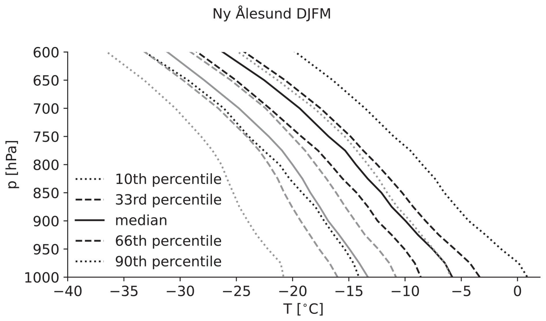
Figure 2 Temperature of air masses originating from the southwest (black lines) and north (grey lines) from radiosonde observations over Ny-Ålesund for DJFM 1993–2014. Profiles of the 10th, 33rd, 50th (median), 66th, and 90th percentiles of temperature at each level are shown.

In contrast to other Arctic wintertime observations (Serreze et al., 1992) and most model results, no climatological temperature inversion emerges in either the median or the percentiles of the observed temperature profiles. The fjord has often remained ice-free throughout the winter in the years covered by our dataset, and radiosonde observations from Danmarkshavn in Greenland (analysis not shown; data available through the Integrated Global Radiosonde Archive (IGRA); Durre et al., 2018) suggest that the presence of upwind topography can cause additional mixing and destroy a temperature inversion that may have existed in the arriving air mass. We therefore do not interpret the deviation of modelled and observed temperatures at lower levels (marked by grey shading in profile plots) as a model bias. These observations might simply not be representative of the scales the models attempt to describe.

As most CMIP6 models do not provide the high-frequency data required to compute these flow-based profiles, we initially evaluate the monthly mean data (Fig. 3). In the free troposphere, a few model results are warmer than observations by 2–3 °C, with one model having a warm bias around 5 °C. Most models have a cold bias of up to 5 °C, and some are cold-biased by nearly 10 °C. The models for which high-frequency data are available (coloured lines) mostly have modest cold biases of 2–3 °C, but MPI-ESM-HAM closely matches observations, and GISS-E2-1-G is among the models with the strongest cold biases around 10 °C. The tendency for a cold bias in the subset of models is thus representative for the CMIP6 ensemble, but models with a warm bias (which are few) and those with stronger but not extreme cold biases around 5 °C are not represented in this subset. For the mean specific-humidity profiles, most models are close to observations, but GISS-E2-1-G (dry) and MPI-ESM-HAM (moist) span a substantial part of the CMIP6 ensemble spread. In the following, we focus on analysing northward- and southward-moving air masses in the subset of models with high-frequency data, bearing in mind that they represent the overall cold bias but not every aspect of the full CMIP6 ensemble.

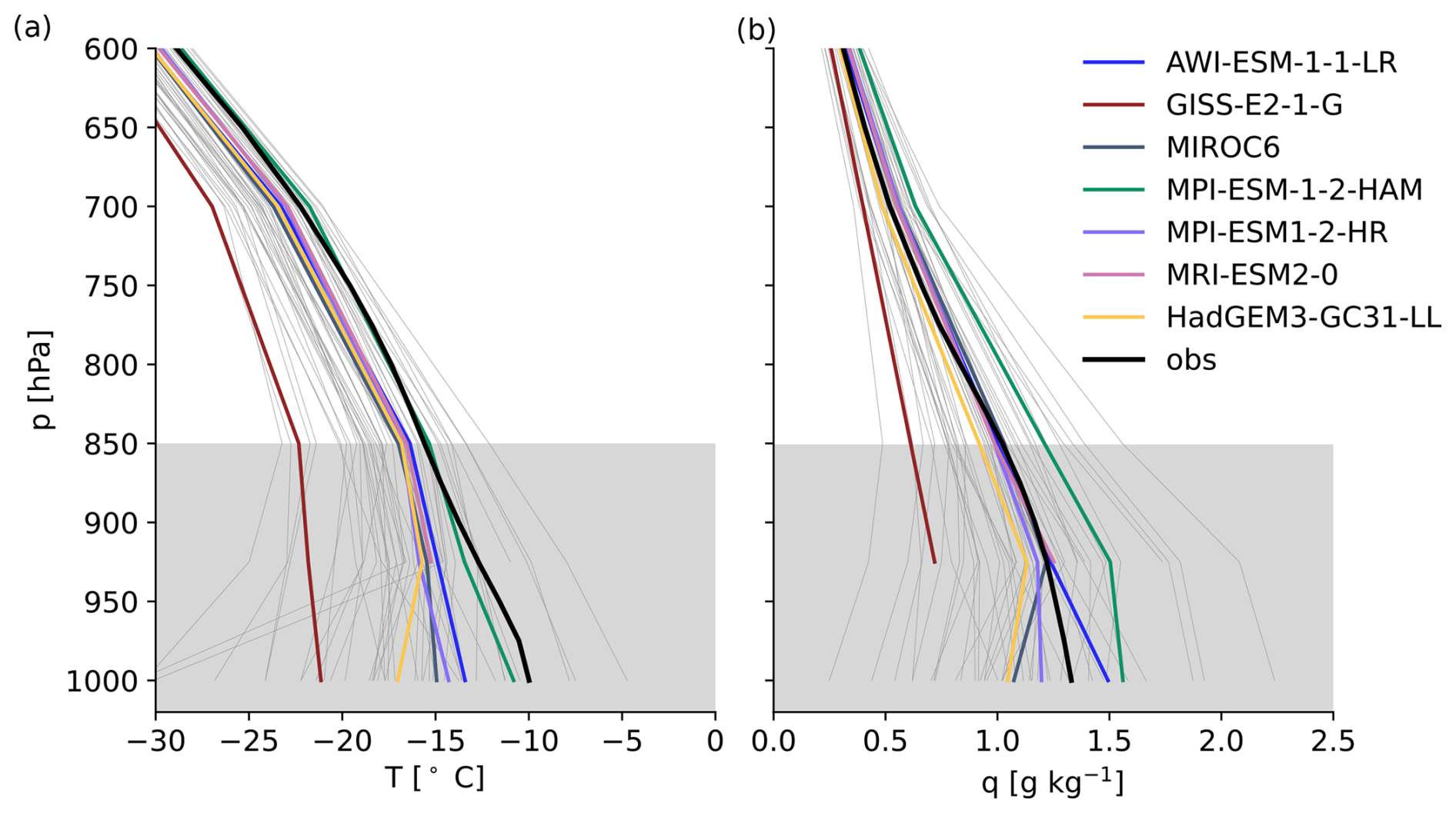
Figure 3 (a) Temperature and (b) specific-humidity profiles from radiosonde observations over Ny-Ålesund and monthly mean output from CMIP6 models for DJFM 1993–2014. Coloured models are those that will be analysed in the remainder of the paper using high-frequency data.

In the free troposphere, i.e. above 850 hPa, models tend to be colder than observed (Fig. 4). This cold bias is somewhat more pronounced in northerly than in southwesterly flows and is generally stronger for the coldest quantiles. The tendency towards a cold bias over Svalbard is consistent with the known near-surface cold bias of CMIP6 models over the central Arctic Ocean in winter (Davy and Outten, 2020).

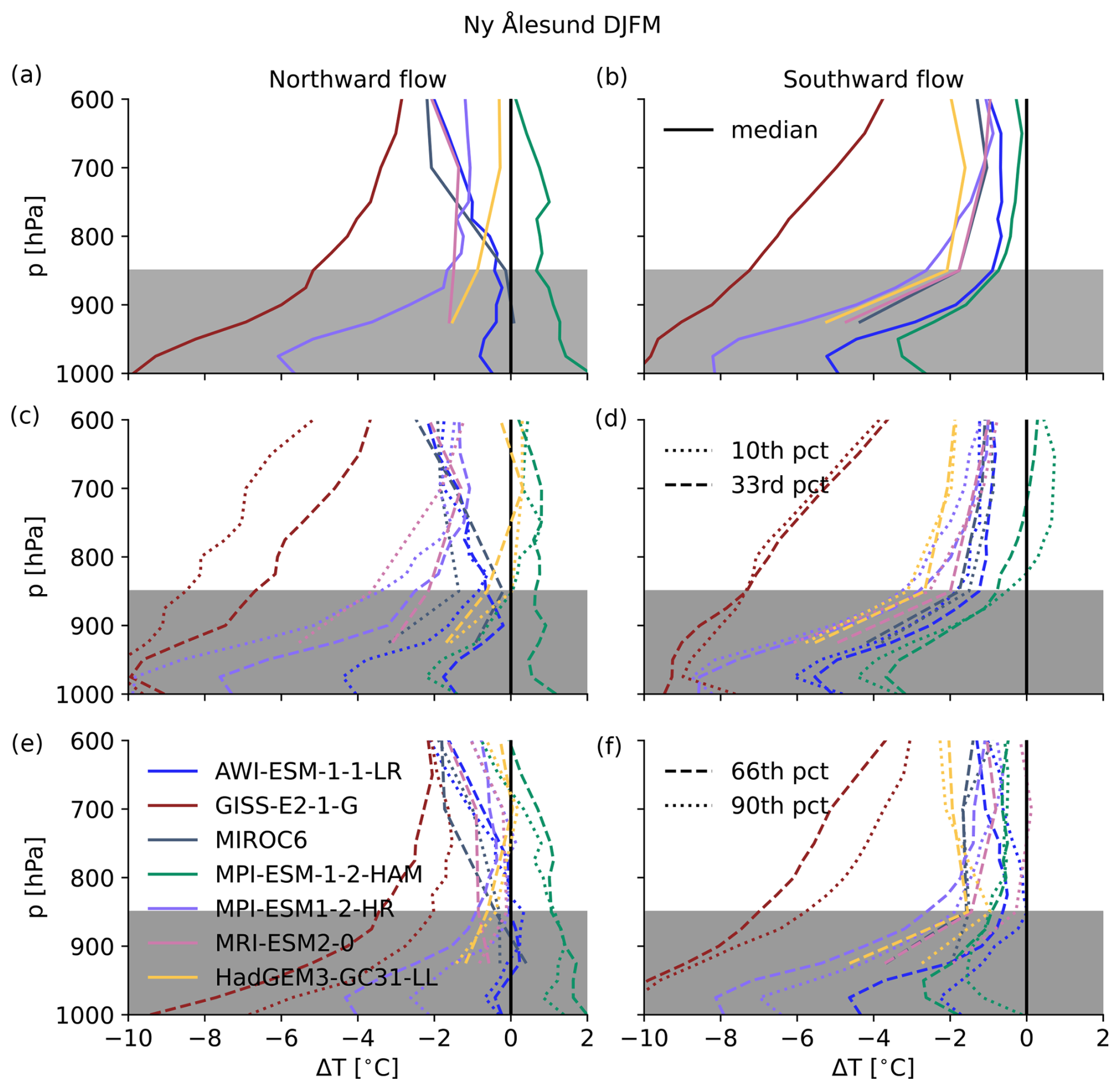
Figure 4 Temperature biases of models against radiosonde observations for air masses originating from the southwest (a, c, e) and from the north (b, d, f) over Ny-Ålesund for DJFM (1993–2014). Biases are shown for the 50th (median, a, b), 10th and 33rd (c, d), and 66th and 90th (e, f) percentiles of temperature at each level. Grey shading marks the altitudes at which we expect strong effects of local topography on the observations that are not represented in the models.

AWI-ESM-1-1-LR matches observed temperatures for the warmest (90th) quantile in air masses flowing poleward in the lower troposphere and only develops a cold bias on the order of 1 °C at 600 hPa. The warmest air masses coming from the south do not show any signs of surface decoupling or temperature inversions in either observations (Fig. 2) or the model (not shown), such that the specific local conditions of the fjord that can cause additional mixing do not lead to a mismatch between observed and AWI-ESM-1-1-LR profiles under these conditions. For colder air masses, especially those advected from the north, AWI-ESM-1-1-LR has a cold bias on the order of 1–2 °C.

GISS-E2-1-G has the most pronounced cold bias among the models analysed here, ranging from 1–2 °C for the warmest air masses in poleward flows to 5–8 °C for air masses coming from the north. The global mean temperature in GISS-E2-1G is largely unbiased, with a compensation between a warm bias at low and southern high latitudes and a pronounced Arctic cold bias (Kelley et al., 2020), suggesting that the cold bias seen in cold Arctic air masses is not just an amplification of a global bias but originates in the middle to high latitudes of the Northern Hemisphere.

MIROC6 has a cold bias on the order of 1–2 °C, which is mostly constant across poleward and equatorward flows and temperature quantiles. Globally, the model is biased warm even when comparing the preindustrial simulation to more recent observations (Tatebe et al., 2019).

MPI-ESM-HAM matches observed temperatures remarkably well in both southwesterly and northerly flows and for all temperature quantiles. In contrast to some of the other models, MPI-ESM-HAM only produces marked temperature inversions in air masses coming from the north.

MPI-ESM-1-2-HR is virtually unbiased for the warmest air masses advected from the south but has a cold bias of at least 2 °C above the temperature inversion for the coldest air masses.

MRI-ESM2-0 matches observed temperatures for the warmest air masses advected from the south and has a cold bias of 1–2 °C above the modelled temperature inversion for the coldest air masses.

HadGEM3-GC31-LL has a weak cold bias in air masses advected from the south and a cold bias of at least 2 °C for air masses advected from the north, with a stronger cold bias for colder quantiles.

Specific humidity in most percentiles increases rapidly towards the surface between 700 and 850 hPa, whereas the increase towards the surface is weaker below 900 hPa (Fig. 5). Near the surface, the moistest poleward-moving air masses contain more than 3 g kg⁻¹ of moisture, roughly twice as much as the moistest air masses drifting southward. The difference in median air masses exceeds a factor of 2.

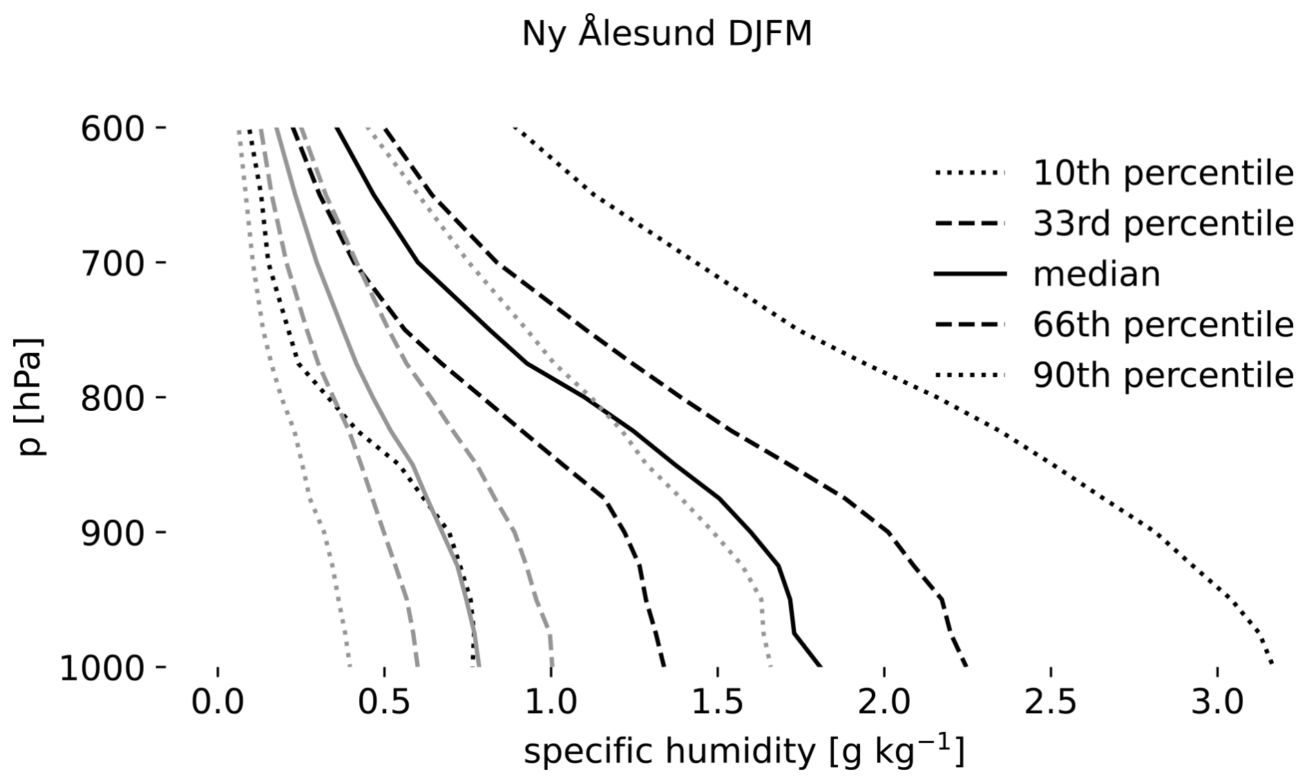
Figure 5 Specific humidity of air masses originating from the southwest (black lines) and north (grey lines) from radiosonde observations over Ny-Ålesund for DJFM 1993–2014. Profiles are shown for the 10th, 33rd, 50th (median), 66th, and 90th percentiles of specific humidity at each level.

Biases in specific humidity (Fig. 6) partly parallel those in temperature, but, as for the monthly mean profiles (Fig. 3), the models do not display a consistent dry bias as could have been expected based on the temperature biases discussed above. Again, the mismatch between observed and modelled profiles in the boundary layer might be due to local conditions in the fjord that do not reflect the large-scale average represented in a model grid box.

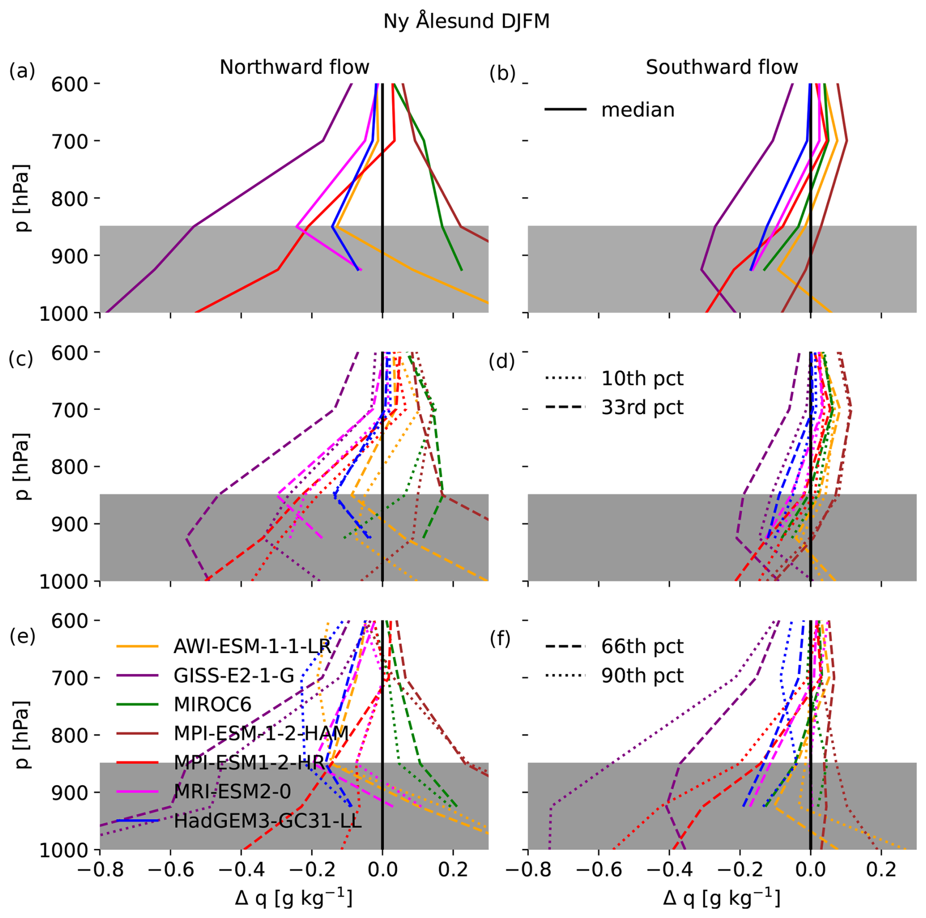
Figure 6 Specific-humidity biases of models against radiosonde measurements for air masses originating from the southwest (a, c, e) and the north (b, d, f) over Ny-Ålesund for DJFM. Biases are shown for the 50th (median, a, b), 10th and 33rd (c, d), and 66th and 90th (e, f) percentiles of specific humidity at each level. Grey shading marks the altitudes at which we expect strong effects of local topography on the observations that are not represented in the models.

AWI-ESM-1-1-LR has a slight dry bias in warm air masses but tends towards a moist bias in cold air masses. GISS-E2-1-G has less humidity than observed under all conditions, consistent with the model's pervasive cold bias discussed above. MIROC6 matches the moisture content of warmer air masses rather well but has a moist bias in cold air masses which is more pronounced than that in AWI-ESM-1-1-LR. Note that MIROC6 has a cold bias under these conditions, suggesting that these air masses must be substantially more saturated in the model than observed in Ny-Ålesund (see the high share of saturated air masses at cold temperatures in MIROC6 in Fig. 8). MPI-ESM-HAM has a tendency towards a moist bias under all conditions, which is more pronounced for the coldest quantiles of air masses being advected equatorwards. MPI-ESM1-2-HR matches observed humidities in the free troposphere rather well. As discussed above, an apparent dry bias in the boundary layer might be due to non-representative conditions in the fjord.

3.2 Relative humidity

To evaluate the relationship between temperature and specific humidity – effectively the relative humidity – in models, we plot specific humidity against temperature (Fig. 7). This avoids any ambiguity with regard to using relative humidity with respect to water or ice and has the added advantage of displaying temperature and humidity at the same time. Below 850 hPa, where most measurements will be influenced by the local boundary layer (Maturilli and Kayser, 2017a), specific humidity is constrained by saturation specific humidity with respect to ice, with substantial variability below that value. This variability is in contrast to measurements from the MOSAiC campaign, where the wintertime boundary layer is much closer to saturation with respect to ice (not shown). We therefore restrict our model evaluation to the lower free-tropospheric levels between 600 and 700 hPa, where observed humidity tends to be either close to or above saturation with respect to ice and bounded by saturation with respect to water or substantially below saturation.

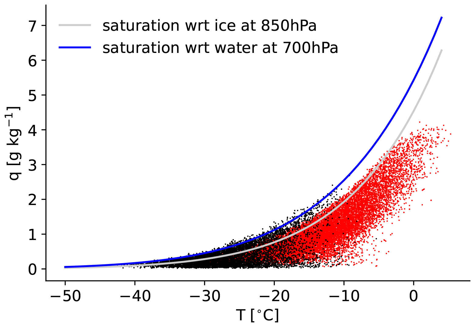
Figure 7 Specific humidity vs. temperature in radiosonde measurements over Ny-Ålesund for DJFM. Each dot represents a single measurement at one time, interpolated to a CMIP pressure level.

Most models are close to saturation with respect to ice for cold temperatures and somewhat below saturation with respect to ice at warmer temperatures (Fig. 8). In particular, at cold temperatures, models tend to lack supersaturated conditions frequently seen in observations. One exception that we will discuss further below is the MRI-ESM2-0 model, which more frequently reaches humidities close to saturation with respect to water – and, thus, supersaturation with respect to ice – at cold temperatures below −15 °C. Several models also lack the strong subsaturation with respect to ice that is seen in observations.

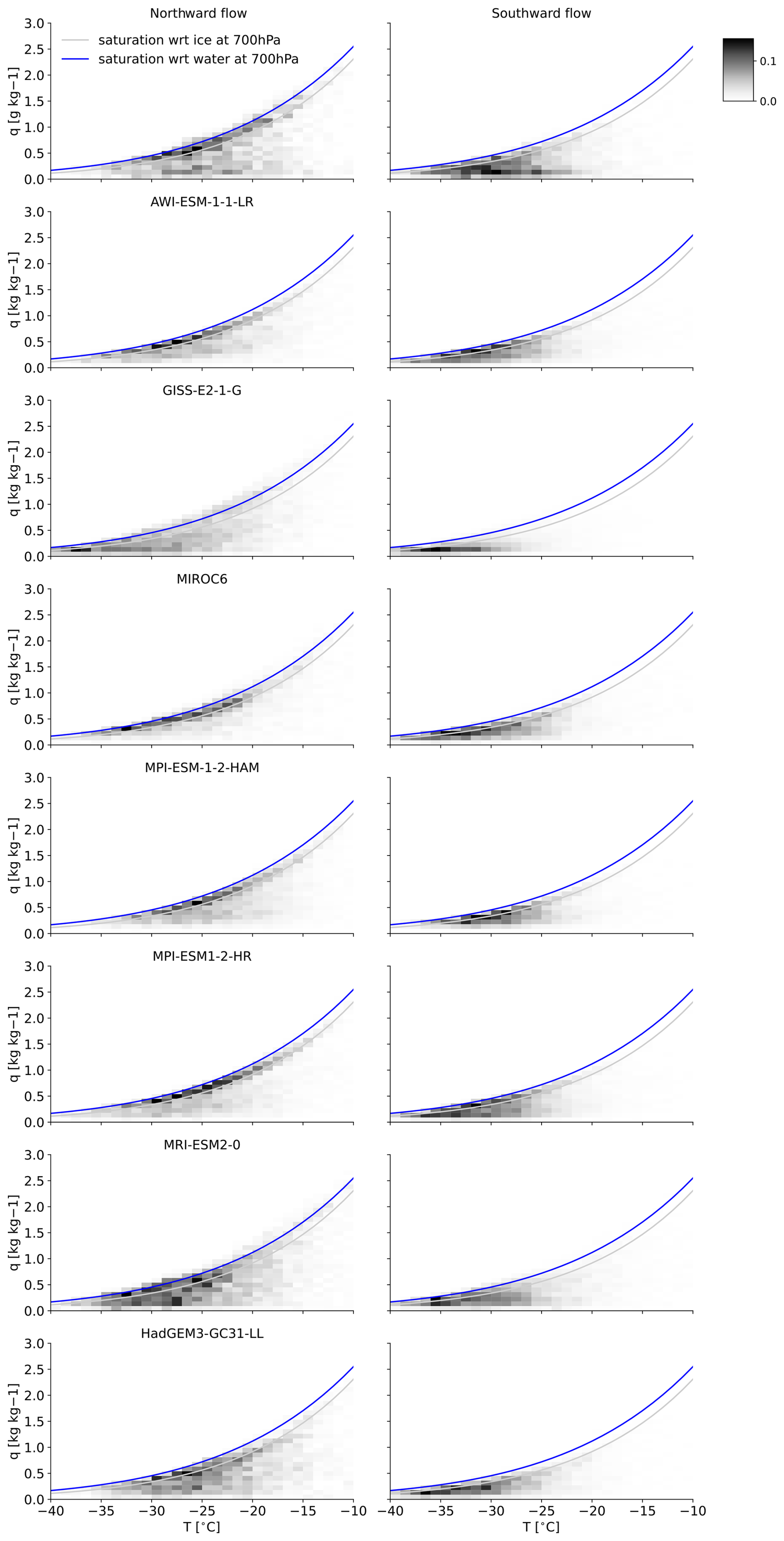
Figure 8 Bivariate pdf of specific humidity vs. temperature in air masses originating from the southwest (left) and the north (right) over Ny-Ålesund for DJFM in radiosonde observations (top row) and climate models.

A larger spread in observed specific humidities compared to modelled specific humidities for a given temperature is to be expected – the radiosonde measurements reflect local conditions right at the sensor of the sonde, whereas the model value is supposed to represent a grid box average. Sub-grid-scale fluctuations of humidity are substantially larger than those of temperature and are accounted for in cloud schemes of large-scale models that produce clouds even when the grid box average is well below saturation (Sundqvist, 1978). We use kilometre-scale model runs following the DYAMOND protocol (Stevens et al., 2019) to investigate to what extent models better capture the observed distribution of relative humidity with respect to ice at higher resolutions, and we vary the microphysics scheme to examine the role of parameterized physics in the distribution (Fig. 9).

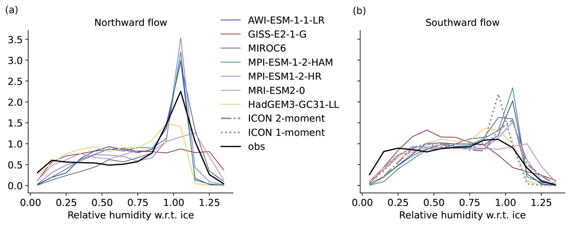
Figure 9 The pdf of saturation with respect to ice for CMIP models and observations over Ny-Ålesund in air masses originating from the southwest (a) and the north (b) during DJFM. ICON data (b) are from a much shorter run compared to CMIP models and cover the central Arctic Ocean (70 to 90° N) to obtain useful statistics. They are plotted alongside observations and CMIP model outputs for air masses originating from the north as they represent air-mass properties in that source region.

In both southwesterly and northerly flows, observed relative humidity with respect to ice is most frequently below 30 % or close to 100 %. Near-saturated conditions are more frequent in southwesterly flows than in northerly flows. Most CMIP models underestimate the occurrence of strong undersaturation and of supersaturation with respect to ice, consistent with the above results for specific humidity compared to temperature.

The lack of supersaturation with respect to ice in the kilometre-scale run is qualitatively similar to the CMIP models when using one-moment microphysics but improves when switching to the two-moment scheme. The CMIP model that most frequently simulates supersaturated conditions under both southwesterly and northerly flows, MRI-ESM2-0, is also one of the few that employs a two-moment microphysics scheme. MPI-ESM-HAM does not substantially outperform MPI-ESM-HR or AWI-ESM-LR in this respect despite having largely the same physics, with the exception of a two-moment microphysics scheme. The GISS model overestimates supersaturation in southwesterly flows and subsaturation in northerly flows.

These results suggest that two-moment microphysics schemes may have an advantage in correctly representing the observed distribution of humidity at and above ice saturation in the Arctic free troposphere. We hypothesize that two-moment schemes can produce low ice number concentrations despite being supersaturated with respect to ice, slowing down the removal of water vapour by depositional growth of ice crystals. In contrast, one-moment schemes would generally tend to diagnose high ice number concentrations under ice supersaturation, which will lead to the quick removal of water vapour.

Ice supersaturation is, indeed, associated with substantially lower ice crystal and snow number concentrations in the ICON two-moment scheme than in the one-moment scheme (Fig. 10; note the logarithmic y axis). We compare the sum of snow and ice number concentrations as both hydrometeor species contribute to the depletion of supersaturation, and the partitioning between both is not consistent between the different microphysics schemes.

Two-moment microphysics schemes thus have a structural advantage over one-moment schemes in representing supersaturation with respect to ice. Other factors in models can also influence the existence or lack of ice supersaturation. For example, the assumption that, in a cold, cloudy grid box, water vapour cannot exceed its saturation value is hard-coded in some models (Tompkins et al., 2007). Such models might still show supersaturated values in the above the probability density function (pdf) due to vertical averaging.

The kilometre-scale ICON runs produce a dry mode with relative humidity with respect to ice below 50 %, which is more similar to observations than the much coarser CMIP models. Comparing the somewhat higher-resolution model MPI-ESM-HR to the physically similar but coarser models MPI-ESM-HAM and AWI-ESM-LR also suggests that a higher horizontal resolution might be helpful in representing low relative humidities, as observed. However, the ICON runs shown here only cover a few days, and, in contrast to the improvement of ice supersaturation with the two-moment scheme, a better representation of the dry mode is not backed up by mechanistic understanding and is regionally less robust (not shown). Whether and why high-resolution models better capture the low relative humidity values should be investigated in future research.

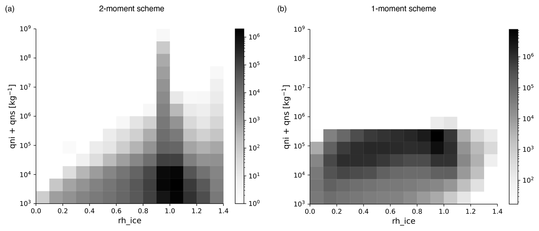
Figure 10 Bivariate pdf of cloud ice and snow number concentration against saturation with respect to ice in the Arctic north of 70° N (a) in the ICON two-moment setup. (b) Diagnostic number concentrations in the one-moment setup. Note the logarithmic y scale and colour scale.

3.3 Longwave radiation

The observed wintertime net longwave radiation in Ny-Ålesund (Fig. 11, defined as positive downwards) shows the bimodal distribution typical of Arctic winter, with a cloudy mode characterized by the presence of cloud liquid water and net surface radiation between 0 and −10 W m⁻² and a clear mode with longwave radiative cooling around −40 W m⁻² (Stramler et al., 2011). The cloudy mode is dominant in air masses arriving from the southwest, confirming that it is caused by the advection and transformation of warm, moist air masses, whereas the clear mode plays a more important role in air masses arriving from the central Arctic Ocean. Consistent with analyses over the central Arctic Ocean (Duffey et al., 2024), not all models appear to reflect this bimodality. But model–observation differences in net radiation may be difficult to interpret as the observational sensor is located over land, whereas some models have a substantial ocean part in the nearest grid box.

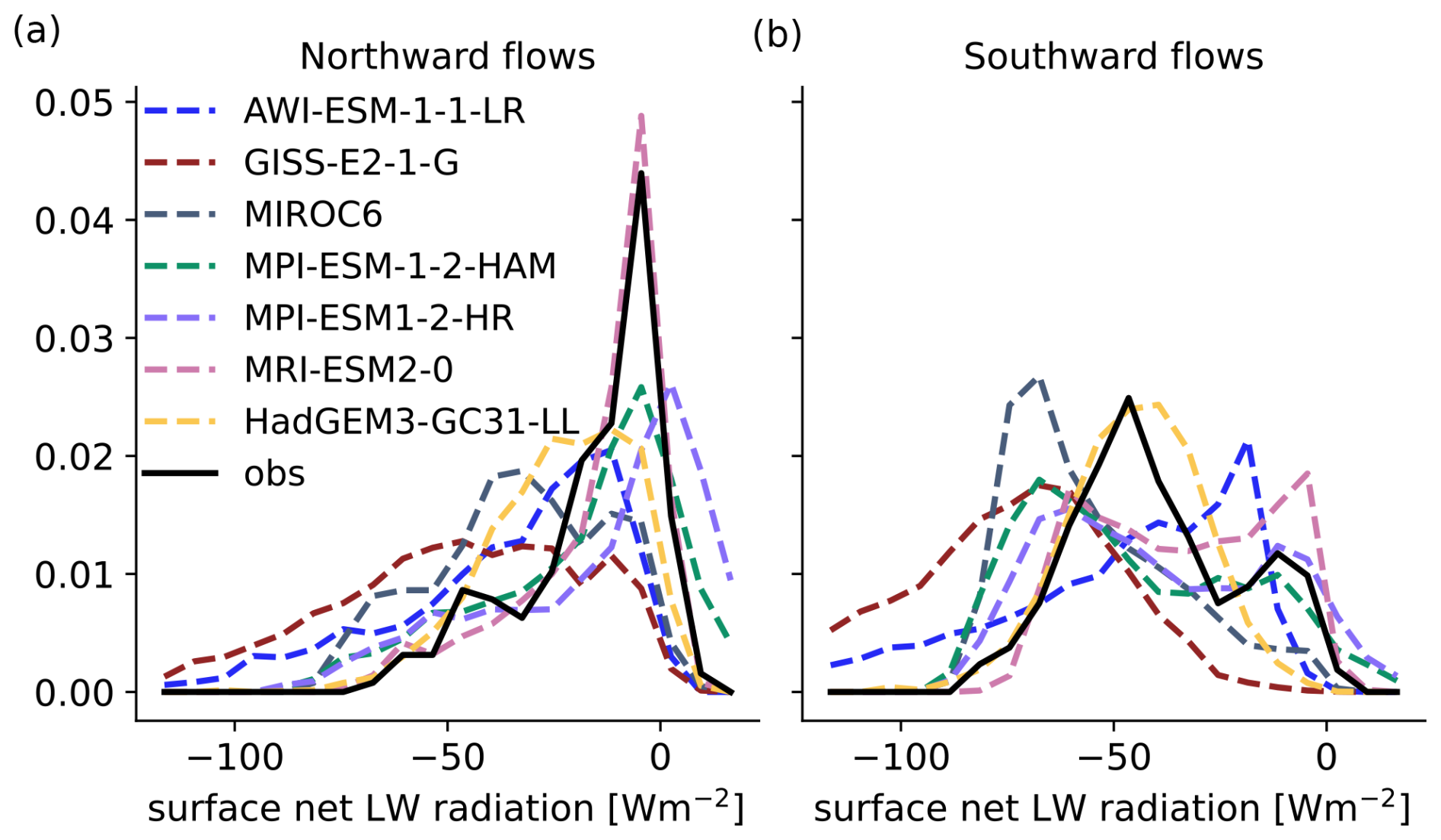
Figure 11 The pdf of net longwave radiation (positive downwards, i.e. towards the surface) in air masses originating from the southwest (a) and the north (b) over Ny-Ålesund for DJFM.

We therefore focus on the downward longwave radiation for further evaluating the models (Fig. 12). In air masses originating from the southwest, models with strong cold biases in the lower troposphere also tend to underestimate downward longwave radiation. However, in air masses coming from the north, some models strongly overestimate downward longwave radiation despite being biased cold in lower-tropospheric temperatures, particularly the GISS model and AWI-ESM-1. As this bias does not seem to be related to the typical temperature profiles of air masses in these models, it has to be associated with the radiative properties of the atmosphere, most likely related to clouds.

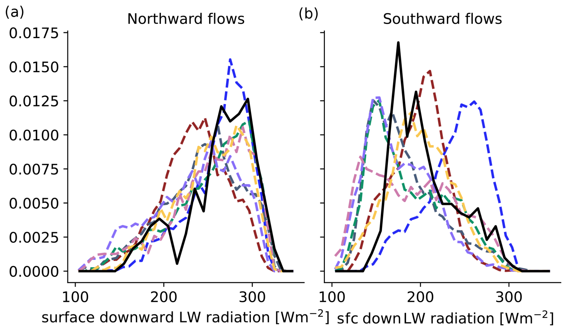
Figure 12 The pdf of downward longwave radiation at the surface in air masses originating from the southwest (a) and the north (b) over Ny-Ålesund for DJFM. Line colours as in Fig. 11.

Plotting temperature at the lowest atmospheric level (925 hPa) against the downward longwave radiation at the surface (Fig. 13) shows two linear relationships corresponding to the bimodal distribution of surface net longwave radiation, with clear-sky emissions at the lower end and fully opaque clouds at the upper end of the distribution. The likelihood of measurements being close to the lower bound, i.e. representing radiatively clear boundary layers, increases at colder temperatures, with the clear state becoming dominant around 265 K. AWI-ESM1-1 appears to show values of downward longwave radiation that exceed the near-linear relationship formed by clouds radiating as blackbodies at a given temperature. We attribute this to the model having its closest grid box over open ocean, whereas all other models for which the land–sea mask was available have a fully or mostly land-covered grid box close to Ny-Ålesund. When choosing the next grid box to the east in AWI-ESM1-1, which is land-covered, the points above the upper bound no longer appear (Fig. 14).

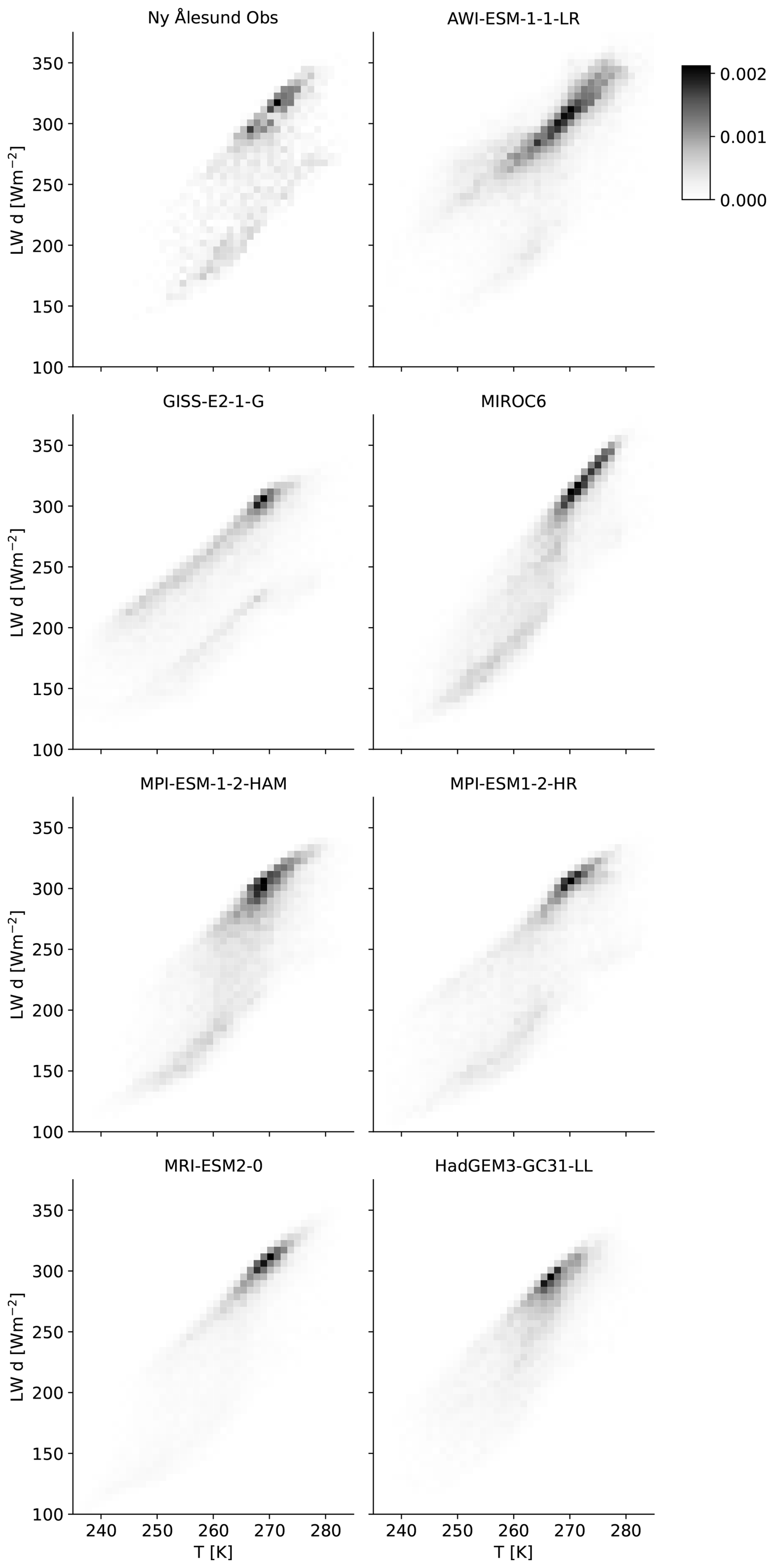
Figure 13 Bivariate pdf of temperature at 925 hPa vs. downward longwave radiation at the surface over Ny-Ålesund for DJFM.

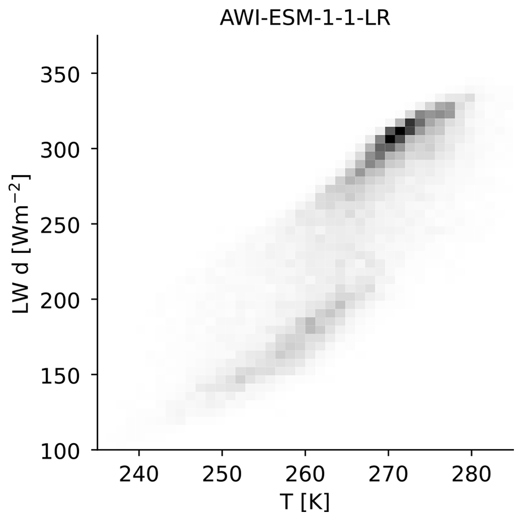
Figure 14 Bivariate pdf of temperature at 925 hPa vs. downward longwave radiation at the surface over Ny-Ålesund for DJFM using a land grid point next to Ny-Ålesund for AWI-ESM-1-1-LR.

In GISS-E2-1-G and, to a lesser extent, in MPI-ESM-HR, the cloudy state of the boundary layer, i.e. values close to the upper bound of downward longwave radiation, is more frequent than observed at temperatures below 265 K. High-emissivity, usually liquid-containing clouds are thus more frequent in these models than in observations at cold temperatures. This is consistent with the finding of Kelley et al. (2020) that the virtual mixed-phase cloud scheme in GISS leads to an overestimation of supercooled liquid compared to satellite observations. For a given tropospheric temperature, more emissive clouds lead to warmer surface temperatures in the Arctic, but they also lead to more efficient radiative cooling of tropospheric air, which could contribute to the strong tropospheric cold bias in GISS-E2-1-G.

While past climate model evaluations often found a lack of supercooled liquid water and high-emissivity clouds at high latitudes (Cesana et al., 2012; Komurcu et al., 2014), here, we see that some CMIP6 models maintain higher cloud emissivity under cold conditions than observed in Ny-Ålesund. This is in agreement with Cesana et al. (2022), who showed that CMIP6 models with a simple, temperature-dependent phase partitioning overestimate liquid in mixed-phase clouds over the Southern Ocean.

3.4 Precipitable water and representativity

Integrating precipitable water from the profiles measured and modelled in southwesterly and northerly flows (Fig. 15) shows that GISS-E2-1G, which is generally cold-biased, has a mode at substantially lower values of precipitable water than observed in southwesterly flows. AWI-ESM-1-1, MPI-ESM-HAM, and MPI-ESM-LR model a realistic distribution of precipitable water in southwesterly flows (Fig. 15a).

In northerly flows (Fig. 15b), GISS-E2-1G produces a mode that is lower than observed, and MPI-ESM-HR has a realistic mode but a lower frequency of occurrence for moister air masses. MPI-ESM-HAM and AWI-ESM1-1 have realistic distributions of precipitable water.

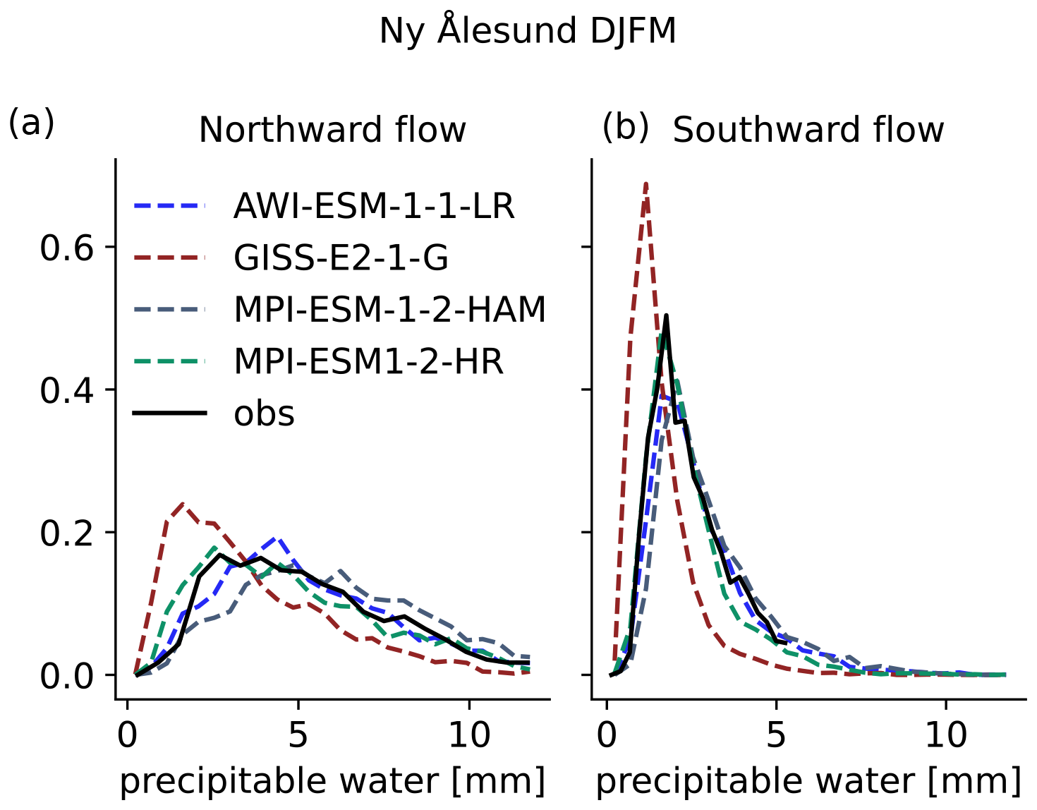
Figure 15 Histogram of modelled and observed values of precipitable water in southwesterly (a) and northerly (b) flows over Ny-Ålesund for DJFM. Models that do not provide data at 1000 hPa are omitted.

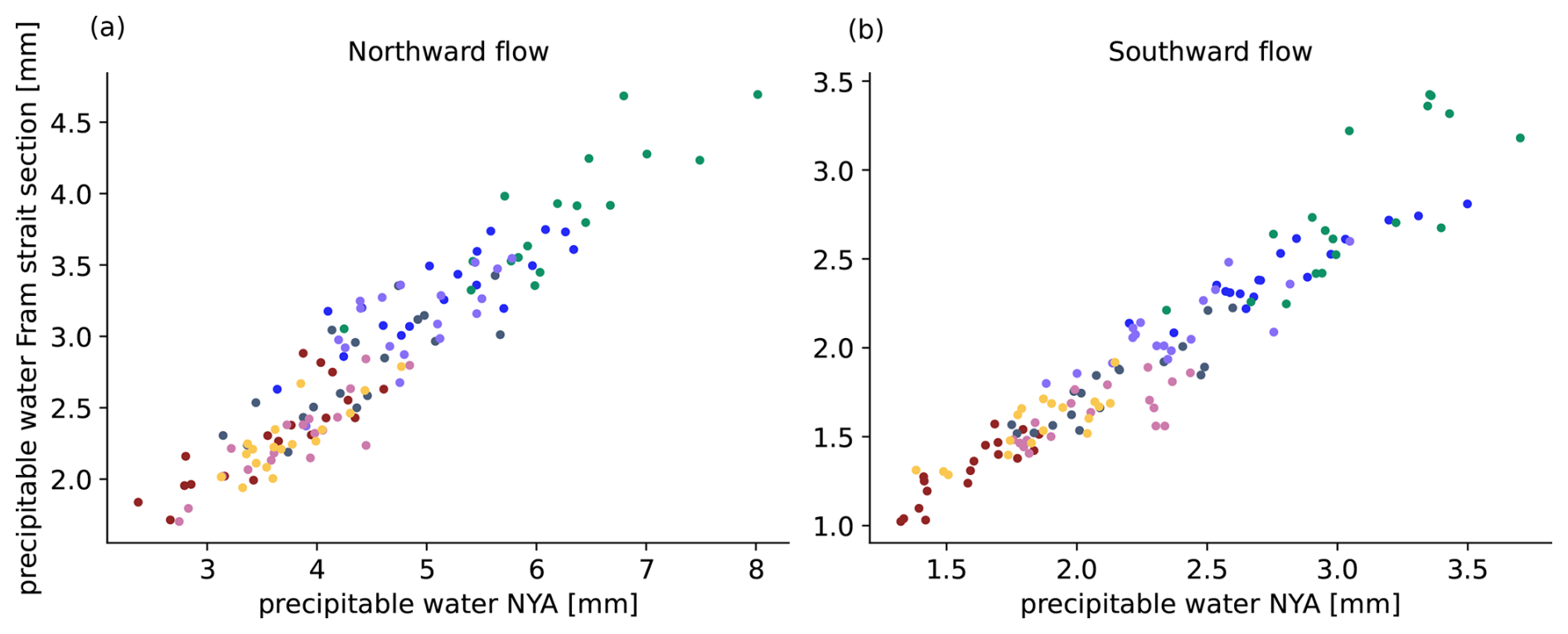
Annual mean values of precipitable water in southwesterly and northerly flows correlate very well between the grid point next to Ny-Ålesund and a section across the Fram Strait in models, both across models and for the interannual variability (Fig. 16). The long-term observations of atmospheric profiles at the AWIPEV research base are thus suitable to evaluate air-mass properties at this crucial gateway to the Arctic in climate models and to record important trends and year-to-year variations in moisture content.

Figure 16 DJFM annual mean of precipitable water modelled for the grid point closest to Ny-Ålesund vs. mean over a section across the Fram Strait for southwesterly (a) and northerly flows (b). Different colours denote different models following the colour coding in Fig. 15.

3.5 Observed trends

The annual mean precipitable water in air masses advected over Ny-Ålesund during DJFM from the southwest has a strong year-to-year variability and an increasing trend of 0.036 mm yr⁻¹, with a p value of 0.056. The 30-year trend (1993–2022) is thus statistically not significant in relation to the standard threshold of 0.05 (Fig. 17a). In air masses advected from the north, a sudden shift towards moister conditions after 2004 stands out from the year-to-year variability. The linear trend is 0.027 mm yr⁻¹, with a p value of less than 0.002, but a linear regression is obviously a poor description of the observed step change. This rapid Arctic wintertime warming and moistening in the early 2000s (Dahlke and Maturilli, 2017) can also be seen in ERA5 precipitable water averaged over the polar cap north of 70° N (Fig. 17b).

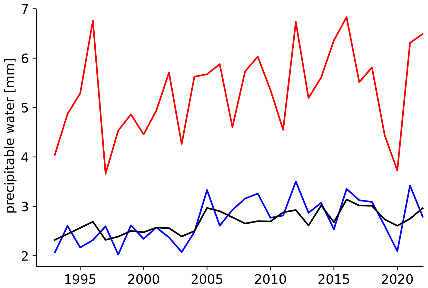
Figure 17 DJFM yearly mean of precipitable water observed over Ny-Ålesund for southwesterly (red) and northerly flows (blue) and DJFM yearly mean of precipitable water in ERA5 averaged over the polar cap north of 70 ° N (black line).

The year 2020 stands out as particularly dry for both southwesterly and northerly flows – it is among the 2 years with the lowest precipitable water values in southwesterly flows and is in line with the low values in northerly flows of the 1990s and earlier 2000s. This is in line with the overall meteorological conditions encountered during the MOSAiC expedition between autumn 2019 and summer 2020, which were dominated by strong zonal flows and little meridional advection which could bring moist air masses to the central Arctic (Lawrence et al., 2020). Measurements in Ny-Ålesund thus reflect the changing conditions over the central Arctic Ocean, including the particular conditions during 2020.

The shift towards moister winter conditions over the central Arctic has been attributed to a more frequent occurrence of southerly winds over the Fram Strait (Dahlke and Maturilli, 2017; Nygård et al., 2020).

4 Summary and conclusions

We compare temperature and moisture in the lower Arctic troposphere as seen in CMIP6 climate models and in observations at Ny-Ålesund, Svalbard, which is located in a major gateway for air-mass exchanges between the Arctic and lower latitudes. We focus on the lower free troposphere as boundary-layer conditions at the measurement site are influenced by the local topography that is not resolved by large-scale models. Climate models tend to be cold-biased (Davy and Outten, 2020), especially for the coldest temperatures, which could be caused by thermodynamic biases or biases in the atmospheric circulation that cause too little exchange of air masses and, thus, too-long residence times of air within the Arctic. Air masses entering the Arctic tend to be less biased or even unbiased in their temperature structure compared to those leaving the Arctic, and Winkelbauer et al. (2024) show that CMIP6 models overestimate atmospheric energy convergence into the Arctic in winter, which suggests that thermodynamic biases are the more likely cause.

Relative humidity in models is more frequently close to saturation over ice in models than in observations. Most models lack supersaturation with respect to ice, and several models also lack subsaturation at relative humidities with respect to ice around or below 30 %. Models with two-moment microphysics that compute rather than assume ice number concentration better represent supersaturation and associate it with lower ice number concentrations. We see some indication that high-resolution models better represent strong subsaturation, but whether and why this is a robust effect remains to be investigated.

As reported from other Arctic wintertime observations (Stramler et al., 2011), the distribution of surface net longwave radiation in Ny-Ålesund is bimodal, representing the clear and cloudy states of the Arctic winter boundary layer. The cloudy state is dominant during southwesterly advection, i.e. for air masses originating over open ocean, and the clear state is dominant for air masses arriving from the sea-ice-covered Arctic Ocean to the north of Svalbard. This bimodal distribution is not represented in all models. Two models substantially overestimate the downward longwave radiation out of cold air masses (in one case, this is despite substantial atmospheric cold biases in these air masses). We attribute this to the cloudy state, with high-emissivity, usually liquid-containing clouds being too frequent at temperatures substantially lower than −10 °C, where the clear state prevails in observations.

Within and across models, the typical moisture content of the atmosphere is strongly correlated between the grid point closest to Ny-Ålesund and a section across the Fram Strait for both southerly and northerly flows. This suggests that the long-term radiosonde observations at Ny-Ålesund capture much of the interannual variability in the properties of air masses passing through this crucial gateway between the Arctic and lower latitudes and that evaluating climate models against the observations provides a meaningful picture of the representation of air-mass properties in models.

The moisture content of air masses arriving in Ny-Ålesund from the north shows a shift towards moister conditions in the early 2000s, which is also evident in reanalysis data averaged over the polar cap. This shift has been attributed to changes in the atmospheric circulation (Dahlke and Maturilli, 2017). The year 2020, i.e. the winter during the MOSAiC expedition, stands out as particularly dry compared to other years after this shift to moister conditions.

We conclude that the near-surface cold bias that occurs in many climate models over the Arctic Ocean in winter is only partly reflected in free-tropospheric temperatures in models with a modest overall cold bias. In all analysed models, the cold bias is much more pronounced for the coldest temperatures than for median temperatures. We recommend further investigating the mechanism behind the frequent occurrence of strong subsaturation and its absence in coarse-resolution models. Finally, our results show that sub-sampling observations from stations around the Arctic Ocean based on wind direction can help to detect trends over the central Arctic Ocean, which is lacking in long-term in situ records.