What can we learn about tropospheric OH from satellite observations of methane?

The hydroxyl radical (OH) is the main oxidant in the troposphere and controls the lifetime of many atmospheric pollutants, including methane. Global annual-mean tropospheric OH concentrations ($\left[\stackrel{\mathrm{‾}}{\mathrm{OH}}\right]$) have been inferred since the late 1970s using the methyl chloroform (MCF) proxy. However, concentrations of MCF are now approaching the detection limit, and a replacement proxy is urgently needed. Previous inversions of GOSAT (Greenhouse Gases Observing Satellite) satellite measurements of methane in the shortwave infrared (SWIR) have shown success in quantifying $\left[\stackrel{\mathrm{‾}}{\mathrm{OH}}\right]$ independently of methane emissions, and observing system simulations have suggested that satellite measurements in the thermal infrared (TIR) may provide additional constraints on OH. Here we combine SWIR and TIR satellite observations from the GOSAT and AIRS instruments, respectively, in a 3-year (2013–2015) analytical Bayesian inversion optimizing both methane emissions and OH concentrations. We examine how much information can be obtained about the interannual, seasonal, and latitudinal features of the OH distribution. We use information from MCF data and the ACCMIP ensemble of global atmospheric chemistry models to construct a full prior error covariance matrix for OH concentrations for use in the inversion. This is essential to avoid an overfitting of the observations. Our results show that GOSAT alone is sufficient to quantify $\left[\stackrel{\mathrm{‾}}{\mathrm{OH}}\right]$ and its interannual variability independently of methane emissions and that AIRS adds little information. The ability to constrain the latitudinal variability of OH is limited by strong error correlations. There is no information on OH at midlatitudes, but there is some information on the $\mathrm{NH}/\mathrm{SH}$ interhemispheric ratio, showing this ratio to be lower than currently simulated in models. There is also some information on the seasonal variation in OH concentrations, although it mainly confirms the variation simulated by the models.

1 Introduction

The hydroxyl radical (OH) is the main oxidant in the troposphere. It determines the lifetimes of most atmospheric species removed by oxidation such as methane (a major greenhouse gas), non-methane volatile organic compounds (NMVOCs, important for air quality), and hydrogenated halocarbons (contributing to stratospheric ozone loss). The global OH concentration and its trend have been monitored indirectly since the 1980s by measuring the concentration of methyl chloroform (MCF), an industrial solvent removed from the atmosphere by reaction with OH (Lovelock, 1977; Prinn et al., 1987; Krol et al., 1998; Bousquet et al., 2005; Patra et al., 2021). MCF was banned in the 1990s because of its contribution to stratospheric ozone depletion, and its concentration is now approaching the detection limit where it loses its value as a proxy for OH (Liang et al., 2017). An observation system simulation experiment (OSSE) previously suggested that a combination of thermal infrared (TIR) and shortwave infrared (SWIR) satellite observations of atmospheric methane could provide a continued proxy for global OH going forward (Zhang et al., 2018). Here we evaluate this idea with a joint inversion of AIRS and GOSAT satellite measurements for 2013–2015, examining the capability of the observations to quantify global OH concentrations and interannual, seasonal, and latitudinal variations.

The OH concentration is controlled by complex photochemistry (Levy, 1971; Logan et al., 1981; Lelieveld et al., 2016). The primary source is UV-B photolysis of ozone in the presence of water vapor. The main sinks are reactions with carbon monoxide (CO), methane, and NMVOCs, resulting in a lifetime of ∼ 1 s and producing peroxy radicals that can be recycled to OH by reaction with nitric oxide (NO). The global-mean tropospheric OH concentration is commonly expressed as the lifetime of methane against oxidation by tropospheric OH, ${\mathit{\tau }}_{{\mathrm{CH}}_{\mathrm{4}}}^{\mathrm{OH}}$. From the methyl chloroform proxy, one infers a tropospheric lifetime of methane of ${\mathit{\tau }}_{{\mathrm{CH}}_{\mathrm{4}}}^{\mathrm{OH}}=$ 11.2 ± 1.3 years for 2000 (Prather et al., 2012). Atmospheric chemistry models find a methane lifetime of ${\mathit{\tau }}_{{\mathrm{CH}}_{\mathrm{4}}}^{\mathrm{OH}}=$ 9.7 ± 1.5 years, implying that OH in the models is too high (Naik et al., 2013).

Although models are generally consistent in their simulations of global-mean OH concentrations, there are large disagreements in the regional distributions of OH concentrations driven by NO_x and NMVOC distributions (Naik et al., 2013; Zhao et al., 2020), chemical mechanisms (Murray et al., 2021), clouds (Liu et al., 2006; Voulgarakis et al., 2009), UV radiation fluxes (Nicely et al., 2020), and other meteorological variables (He et al., 2021). Models consistently simulate higher OH in the Northern Hemisphere (NH) than the Southern Hemisphere (SH) (Naik et al., 2013; Stevenson et al., 2020). MCF observations, by contrast, suggest no interhemispheric gradient (Patra et al., 2014) or slightly higher OH in the SH (Montzka et al., 2000). Models may have excessive OH in the Northern Hemisphere because of underestimated CO (Naik et al., 2013).

Understanding year-to-year variability and decadal-scale trends in OH concentrations is important for attributing the cause of methane fluctuations (Turner et al., 2017), including the recent acceleration of the methane trend (Laughner et al., 2021; Qu et al., 2022; Stevenson et al., 2022). Methane is emitted from a range of poorly quantified sources, including wetlands, livestock, waste, fuel exploitation, rice paddies, and open fires (Saunois et al., 2020). These sources could be responsible for methane interannual variability and trends, but OH concentrations could also be responsible (Turner et al., 2017). The El Niño–Southern Oscillation (ENSO) drives interannual variability in model OH due to its influence on lightning (Murray et al., 2013; Turner et al., 2018; Anderson et al., 2021), water vapor (Turner et al., 2018; Anderson et al., 2021), and CO emitted from biomass burning (Zhao et al., 2020). Models and measurements show a 5 % range of interannual variability of OH over the last 30 years, albeit with no temporal correlation between the two (Szopa et al., 2021). Models find increasing OH from 1980 to present driven by increases in anthropogenic NO_x emissions (Naik et al., 2013; Gaubert et al., 2017; Zhao et al., 2019; Stevenson et al., 2020). By contrast, MCF observations indicate OH increasing from 1980 to 2005 but then flat or decreasing after 2005 (Rigby et al., 2017; Turner et al., 2017; Nicely et al., 2018; Stevenson et al., 2020).

Many studies have used satellite observations of methane to infer methane emissions using specified OH concentrations to optimize methane sources (Turner et al., 2015), while others have attempted to optimize both methane sources and OH concentrations by exploiting differences in spatial and seasonal impacts on methane concentrations (Maasakkers et al., 2019; Zhang et al., 2021) (Maasakkers et al., 2016; Zhang et al., 2021) or by including complementary information in the inversion from observations of MCF (Cressot et al., 2014, 2016) or formaldehyde and CO (Yin et al., 2021). Inversions of GOSAT (SWIR) satellite observations of methane alone can constrain global-mean OH about as well as MCF and infer a flat interhemispheric gradient, although posterior errors may be too optimistic (Maasakkers et al., 2019; Lu et al., 2021; Zhang et al., 2021). Zhang et al. (2018) proposed that TIR satellite observations of methane, which have sensitivity to the free troposphere and broader coverage over oceans and at night, may reduce error correlation between OH and methane emissions.

Satellite-based observations of methane in the TIR have been made continuously since 2002 by several instruments: AIRS (2002–present), TES (2004–2011), IASI (2007–present), CrIS (2011–present), and GOSAT-2 (2018–present) (Jacob et al., 2016). TIR observations have received little attention in inverse studies because they are not sensitive to methane near the surface (Wecht et al., 2012). Direct applications of TIR satellite observations have mostly focused on processes affecting the free troposphere, such as detecting stratospheric intrusions (Xiong et al., 2013), methane emissions from large wildfires (Xiong et al., 2010; Ribeiro et al., 2018), interannual variations in mid-troposphere methane in response to ENSO (Corbett et al., 2017), seasonal fluctuations in methane in response to fossil fuel and rice paddy emissions in China (Zhang et al., 2011), and differences in seasonality compared to surface observations (Zhou et al., 2023). The combination of SWIR and TIR observations has been used to develop lower troposphere methane products including those using GOSAT + AIRS (Worden et al., 2015), GOSAT + IASI (Schneider et al., 2022), and GOSAT-2 (Kuze et al., 2022; Suto, 2022).

Here we combine TIR observations from AIRS with SWIR observations from GOSAT in a 3-year 2013–2015 inversion optimizing both methane emissions and OH concentrations. We use an analytical solution that provides formal characterization of posterior error statistics (including error correlations) and information content as part of the inversion. We place particular focus on the ability of the inversion to quantify global-mean OH concentrations, interannual variability, and latitudinal and seasonal variations. This involves careful characterization of prior error covariances using OH concentrations from the ACCMIP model ensemble (Naik et al., 2013).

2 Data and methods

We use 3 years (2013–2015) of satellite observations from GOSAT and AIRS (Sect. 2.1) to optimize a state vector of OH distributions and annual methane emissions. The observations are assembled in an observation vector y with total dimension m. The state vector x comprises n elements describing annual gridded non-wetland methane emissions, monthly subcontinental wetland methane emissions, and mean OH concentrations for individual years in different latitudinal bands and seasons (Sect. 2.2). Optimization is done by Bayesian inference using a prior estimate x_A for the state vector and error covariances for that prior estimate (S_A) and for the observations (S_O) (Sect. 2.3), together with the GEOS-Chem chemical transport model y = F(x), expressing the sensitivity of the observations to the state vector (Sect. 2.4). We use an analytical solution for minimization of the Bayesian cost function J(x) to yield the optimal value (posterior estimate) $\widehat{\mathit{x}}$ of the state vector, the posterior error covariance matrix $\widehat{\mathbf{S}}$, and metrics of information content (Sect. 2.5). The subsections below describe these different elements of the inversion, with the exception of the prior error covariance matrix of OH concentrations, which will be presented in a dedicated Sect. 3. Throughout this paper, we refer to “OH concentrations” ([OH]) for a given domain as the mass-weighted average tropospheric OH number density for that domain and the global annual-mean tropospheric OH concentrations as $\left[\stackrel{\mathrm{‾}}{\mathrm{OH}}\right]$.

2.1 Satellite data

GOSAT (Greenhouse Gases Observing Satellite), launched in 2009, detects methane by solar backscatter in the SWIR using the TANSO-FTS (Thermal and Near Infrared Sensor for Carbon Observation – Fourier Transform Spectrometer) instrument. In its default operating mode, GOSAT provides 10.5 km diameter nadir observations of radiance separated by about 250 km along-track and cross-track on a sun-synchronous orbit with an equatorial overpass at about 13:00 local solar time (LST). We use the University of Leicester CO₂ proxy methane retrieval v9.0 (Parker and Boesch, 2020), which uses the GOSAT observations in the 1.65 µm band to retrieve methane as a column-averaged dry-air mixing ratio $X_{{\mathrm{CH}}_{\mathrm{4}}}$ with a vertical sensitivity profile (column averaging kernel) of near unity in the troposphere.

AIRS (Atmospheric Infrared Sounder), launched in 2002, detects methane by observing TIR radiation emitted by the Earth. AIRS provides 15 km diameter nadir observations across a 1250 km swath with equatorial overpasses at about 01:30 and 13:30 LST, resulting in global coverage twice per day. We use the optimal estimation MUSES-AIRS retrieval of methane in the 8 and 12 µm bands, which provides 26-level profiles of the dry-air methane mixing ratio (Kulawik et al., 2021). The AIRS instrument has less than 2 degrees of freedom for the signal per measurement and little sensitivity to the lower troposphere. We therefore convert the vertical profiles to a column-averaged dry-air mixing ratio $X_{{\mathrm{CH}}_{\mathrm{4}}}$ above 600 hPa, with column averaging kernels featuring maximum sensitivity to the upper troposphere. See Worden et al. (2015) for typical GOSAT and AIRS column averaging kernels.

For both AIRS and GOSAT, we remove measurements flagged for low-quality, negative values and surface pressures differing by more than 50 hPa from the local GEOS-Chem surface pressure that would indicate unresolved topography. We do not use GOSAT sunglint measurements because of their sparsity and seasonal sampling bias (Maasakkers et al., 2019). We also exclude measurements poleward of 60° due to model stratospheric bias in interpreting methane column observations in the polar vortex (Turner et al., 2015; Stanevich et al., 2020; Zhang et al., 2021). We include both daytime and nighttime measurements for AIRS, as we find no significant biases between them. This results in 600 000 successful retrievals for GOSAT and 2.5 million for AIRS.

In order to compare satellite retrievals to the GEOS-Chem simulations, we produce a model column sampled in the same manner as the satellite data. For each AIRS and GOSAT observation, we select the coincident GEOS-Chem grid cell and interpolate the GEOS-Chem methane mixing ratio profile, which is on 47 vertical levels, to the AIRS profile (26 vertical levels) and the GOSAT profile (20 vertical levels) using a mass-conserving interpolation algorithm described in Keppens et al. (2019) and by the General Observation Operator for Python (GOOPy) v0.1.0 (https://doi.org/10.5281/zenodo.14834528, Penn and Nesser, 2025). We call these interpolated profiles c_m. We then translate these profiles to column-averaged dry-air mixing ratios using the column averaging kernel a. The column averaging kernel is based on mixing ratio and does not include different pressure weights for each level (Boesch et al., 2011), so we apply the pressure weighting function (h) provided in the GOSAT and AIRS data products. For an individual satellite $X_{{\mathrm{CH}}_{\mathrm{4}}}$ observation y, we derive the corresponding model value y_m using

$$\begin{array}{}\text{(1)}& y_{\mathrm{m}}={\mathit{h}}^T\left((\mathbf{I}-\mathbf{A}){\mathit{c}}_a+\mathbf{A}{\mathit{c}}_{\mathrm{m}}\right),\end{array}$$

where I is the identity matrix, A is the diagonal averaging kernel matrix with the elements of a as diagonal elements, and c_a is the prior profile provided by the GOSAT and AIRS products, which come from the MACC-II methane inversion and TOMCAT stratospheric chemistry model for GOSAT and from the MOZART atmospheric chemistry model for AIRS.

Figure 1 shows satellite observations from 2013 for GOSAT and AIRS compared to a 2013 GEOS-Chem simulation driven by GOSAT-optimized emissions from Lu et al. (2021). As expected, GOSAT is globally unbiased relative to this GEOS-Chem simulation (−2 ± 12 ppb), but AIRS is biased low (−19 ppb ± 24 ppb), and thus we apply a correction of +19 ppb to the AIRS data to ensure consistency with GOSAT. Although errors in the GEOS-Chem vertical profiles of methane mixing ratios would affect this intercomparison platform, we see in Fig. 1 that the AIRS bias extends over background regions where the vertical profile would be uniform. Figure 1 shows additional latitudinal differences between AIRS and GOSAT, but these may provide information for the inversion, and we have no rationale to remove them.

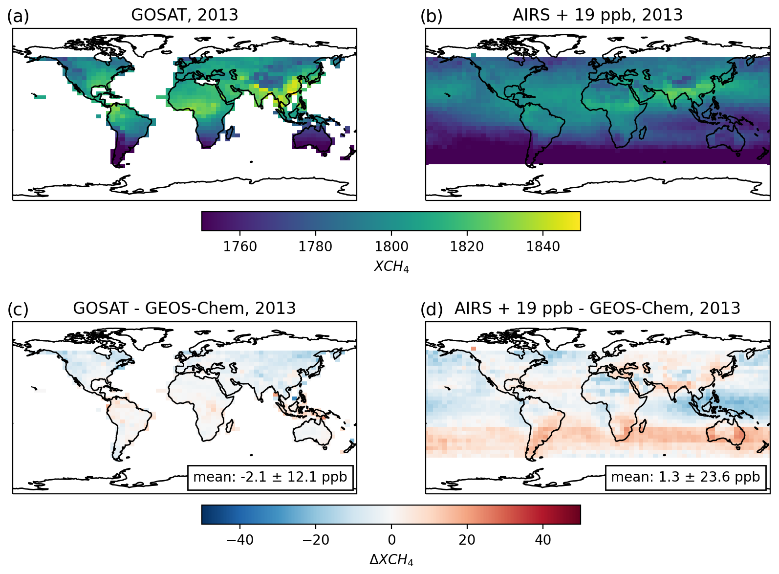
Figure 1 GOSAT and AIRS observations of annual-mean methane dry-column mixing ratio ($X_{{\mathrm{CH}}_{\mathrm{4}}}$) in 2013, binned by 4° × 5° grid cells. GOSAT sunglint and observations poleward of 60° are not included. The bottom panels compare these observations with a GEOS-Chem simulation driven by 2013 posterior emissions from an inversion of GOSAT observations (Lu et al., 2021). A +19 ppb global bias correction is applied to AIRS on the basis of this comparison. Means and standard deviations of the differences between the satellite observations and GEOS-Chem are given inset.

2.2 State vector and prior estimates

We optimize a state vector including annual gridded non-wetland emissions, monthly subcontinental wetland emissions, and OH distributions. Separate characterization of wetland and non-wetland emissions is done on the basis of assumed subcontinental spatial coherence and seasonality of the prior wetland emission estimates (Maasakkers et al., 2019; Zhang et al., 2021). Non-wetland emissions consist of 1009 total 4° × 5° grid cells over land for each year (1009 × 3 = 3027 elements). Wetland emissions are optimized for each month and in 14 subcontinental regions following Bloom et al. (2017) (12 × 14 × 3 = 504 elements). OH concentrations are optimized for each season and year in four latitude bands of 30° each from 60° S to 60° N (4 × 4 × 3 = 48 elements). This results in n= 3579 total state vector elements.

We define $\mathbf{K}=\partial y/\partial x$ as the m×n Jacobian matrix describing the dependence of satellite observations on the state vector as simulated by GEOS-Chem. We calculate the Jacobian by perturbing each element of the state vector by 50 % (for emissions) and 20 % (for [OH]), resulting in $n+\mathrm{1}=\mathrm{3580}$ forward model runs. This calculation is insensitive to the magnitudes of the perturbations because the forward model is strictly linear in the relationship of concentrations to emissions, and the assumption of linearity is also acceptable for the relationship to OH concentrations in a 3-year simulation. Thus, K fully defines GEOS-Chem for the purpose of the inversion.

The state vector elements are optimized in the inversion as scaling factors relative to prior estimates. We use the same prior estimates as Lu et al. (2021). Default prior anthropogenic emissions are from the EDGAR inventory v4.3.2 (Crippa et al., 2018) and are superseded for the US by the gridded EPA inventory of Maasakkers et al. (2016) and globally for oil, gas, and coal by the GFEI inventory of Scarpelli et al. (2020). Prior anthropogenic emissions are assumed to be constant, with the exception of manure and rice for which we apply seasonal scaling factors (Maasakkers et al., 2016; Zhang et al., 2016). Prior wetland emissions are from WetCHARTS v1.0 with 0.5° × 0.5° spatial resolution and monthly temporal resolution, spatially aggregated into 14 subcontinental regions for use in inversions (Bloom et al., 2017). Additional prior emissions include the GFED inventory for fires at daily resolution (Randerson et al., 2017) and geologic sources from Etiope et al. (2019) scaled to the global total from Hmiel et al. (2020). Prior tropospheric OH concentrations (Fig. 2) are archived monthly mean values from an older (version 5) GEOS-Chem simulation on the 4° × 5° grid (Wecht et al., 2014). The mass-weighted annual-mean tropospheric OH concentration is $\left[\stackrel{\mathrm{‾}}{\mathrm{OH}}\right]=\mathrm{11.2}\times {\mathrm{10}}^{\mathrm{5}}$ molec. cm⁻³, consistent with the MCF-derived estimate from 2000 of $\left[\stackrel{\mathrm{‾}}{\mathrm{OH}}\right]={\mathrm{10.8}}_{-\mathrm{0.85}}^{+\mathrm{0.77}}\times {\mathrm{10}}^{\mathrm{5}}$ molec. cm⁻³ (Prinn et al., 2005). More recent versions of GEOS-Chem overestimate $\left[\stackrel{\mathrm{‾}}{\mathrm{OH}}\right]$ (Shah et al., 2023), as also seen in other current models (Stevenson et al., 2020).

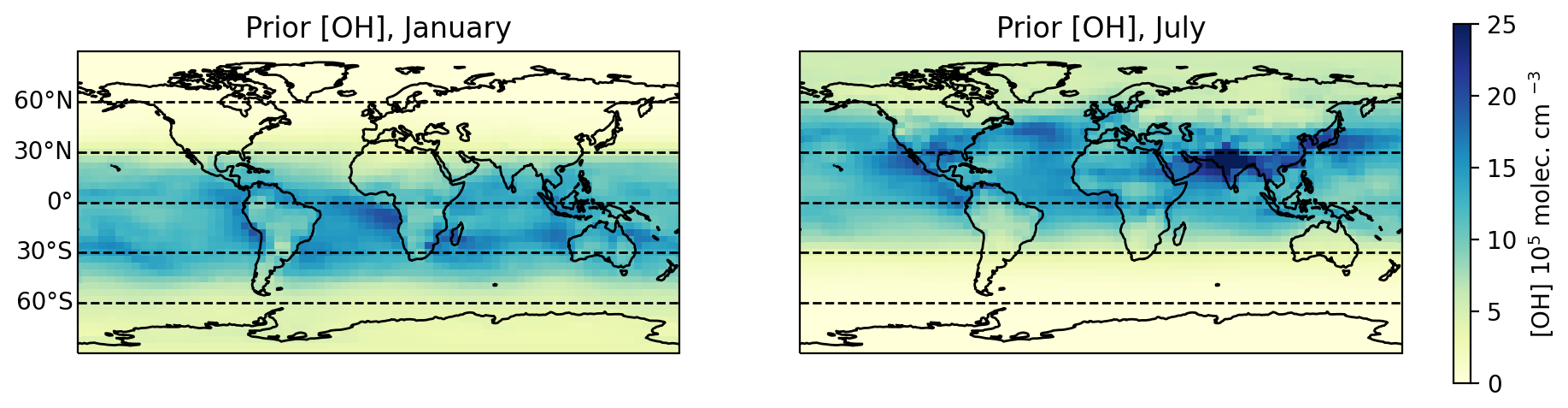
Figure 2 Mass-weighted tropospheric OH concentrations in GEOS-Chem (tropospheric columns) used as prior estimates for the inversions. Monthly mean values for January and July are shown.

2.3 Error estimates

The inversion requires specification of both observing system and prior error covariance matrices. The observing system error includes contributions from the measurement and from the forward model. We use the residual error method described in Heald et al. (2004) to derive it. We first split the observations into monthly 4° × 5° grid cell subsets and compare observations within each subset to the GEOS-Chem simulation F(x) using prior values. We then assume that the model bias ($b=\stackrel{\mathrm{‾}}{\mathbf{F}\left({\mathit{x}}_{\mathrm{A}}\right)-y}$) within each subset is due to error in the prior estimates and that the residual represents the observing system error. In this manner we find mean observing system error standard deviations of 12 ppb for GOSAT and 22 ppb for AIRS, mostly attributed to the retrieval error, with reported error standard deviations averaging 10 ppb for GOSAT and 16 ppb for AIRS. Our observing system error standard deviation for GOSAT is consistent with previous estimates (e.g., Lu et al., 2021; Qu et al., 2021; Zhang et al., 2021). We construct the observing system error covariance matrix assuming no error correlation between individual observations (diagonal matrix).

Prior error standard deviations for non-wetland emissions are assumed to be 50 % of emissions for each 4° × 5° grid cell with no error covariance between grid cells, as in previous studies (Maasakkers et al., 2019; Zhang et al., 2021). The effect of this prior error is reflected in the averaging kernel sensitivities. For wetland emissions, we calculate the full prior error covariance matrix between all 14 regions and 36 months from the WetCHARTs model ensemble following Bloom et al. (2017) and then shrink the off-diagonal terms following Schäfer and Strimmer (2005) to ensure that the matrix is positive-definite. Prior error estimates for the OH elements of the state vector are derived in Sect. 3.

2.4 Forward model

We use the GEOS-Chem version 12.7.1 CH₄ simulation (https://doi.org/10.5281/zenodo.3676008, Developers of GEOS-Chem, 2020) on a 4° × 5° grid with 47 vertical layers as forward model for the inversion. Atmospheric transport is driven by the Modern-Era Retrospective Analysis for Research and Applications, version 2 (MERRA-2), assimilated meteorological fields for 2013–2015 from the NASA Global Modeling and Assimilation Office. In addition to the tropospheric OH fields optimized in the inversion (Sect. 2.2), minor methane sinks in GEOS-Chem include stratospheric loss prescribed with 2-D oxidant fields (Murray et al., 2013), oxidation by tropospheric Cl following Wang et al. (2019), and soil uptake from the MeMo inventory (Murguia-Flores et al., 2018). Initial conditions for 1 January 2013 come from the GOSAT-optimized posterior simulation of Lu et al. (2021) and are globally unbiased with respect to GOSAT and adjusted AIRS observations as described in Sect. 2.1.

2.5 Inversion

We perform three inversions: “GOSAT-only”, which is optimized with GOSAT observations; “AIRS-only”, which is optimized with AIRS observations; and “GOSAT + AIRS”, which is optimized with both. The equations below are for the inversion using both GOSAT and AIRS observations. Because we assume no error correlations between the instruments, an inversion with only one instrument can be derived by removing all terms pertaining to the other instrument.

We minimize a Bayesian cost function that accounts for the distance from the prior estimate (x_A) and the satellite observations (y) that is weighted by the inverse of the prior (S_A) and observing system (S_O) error covariance matrices and includes an additional regularization factor (γ). Observing system components from GOSAT and AIRS are denoted by subscripts. Assuming normal errors and no correlation between GOSAT and AIRS errors, the cost function is given by

$$\begin{array}{}\text{(2)}& \begin{array}{rl}J\left(\mathit{x}\right)& ={\left(\mathit{x}-{\mathit{x}}_{\mathrm{A}}\right)}^T{\mathbf{S}}_{\mathrm{A}}^{-\mathrm{1}}\left(\mathit{x}-{\mathit{x}}_{\mathrm{A}}\right)\\ & +{\mathit{\gamma }}_{\mathrm{GOSAT}}{\left({\mathit{y}}_{\mathrm{GOSAT}}-{\mathbf{K}}_{\mathrm{GOSAT}}\mathit{x}\right)}^T{\mathbf{S}}_{\mathrm{O},\mathrm{GOSAT}}^{-\mathrm{1}}\\ & \left({\mathit{y}}_{\mathrm{GOSAT}}-{\mathbf{K}}_{\mathrm{GOSAT}}\mathit{x}\right)+{\mathit{\gamma }}_{\mathrm{AIRS}}{\left({\mathit{y}}_{\mathrm{AIRS}}-{\mathbf{K}}_{\mathrm{AIRS}}\mathit{x}\right)}^T\\ & {\mathbf{S}}_{\mathrm{O},\mathrm{AIRS}}^{-\mathrm{1}}({\mathit{y}}_{\mathrm{AIRS}}-{\mathbf{K}}_{\mathrm{AIRS}}\mathit{x})\end{array}.\end{array}$$

We can then solve min(J(x)) analytically by setting $\partial J/\partial x=\mathrm{0}$ and obtain the posterior solution $\widehat{\mathit{x}}$ (Rodgers, 2000):

$$\begin{array}{}\text{(3)}& \begin{array}{rl}\widehat{\mathit{x}}& ={\mathit{x}}_{\mathrm{A}}+{\mathbf{G}}_{\mathrm{GOSAT}}\left({\mathit{y}}_{\mathrm{GOSAT}}-{\mathbf{K}}_{\mathrm{GOSAT}}{\mathit{x}}_{\mathrm{A}}\right)\\ & +{\mathbf{G}}_{\mathrm{AIRS}}\left({\mathit{y}}_{\mathrm{AIRS}}-{\mathbf{K}}_{\mathrm{AIRS}}{\mathit{x}}_{\mathrm{A}}\right)\end{array},\end{array}$$

where $\widehat{\mathit{x}}$ is the posterior estimate for the state vector and G_AIRS and G_GOSAT are the gain matrices:

$$\begin{array}{}\text{(4)}& \begin{array}{rl}{\mathbf{G}}_{\mathrm{AIRS}}& ={\mathbf{S}}_{\mathrm{A}}{\mathbf{K}}_{\mathrm{AIRS}}^T{\left({\mathbf{K}}_{\mathrm{AIRS}}{\mathbf{S}}_{\mathrm{A}}{\mathbf{K}}_{\mathrm{AIRS}}^T+{\displaystyle \frac{\mathrm{1}}{{\mathit{\gamma }}_{\mathrm{AIRS}}}}{\mathbf{S}}_{\mathrm{O},\mathrm{AIRS}}\right)}^{-\mathrm{1}}\\ & {\mathbf{G}}_{\mathrm{GOSAT}}={\mathbf{S}}_{\mathrm{A}}{\mathbf{K}}_{\mathrm{GOSAT}}^T\\ & {\left({\mathbf{K}}_{\mathrm{GOSAT}}{\mathbf{S}}_{\mathrm{A}}{\mathbf{K}}_{\mathrm{GOSAT}}^T+{\displaystyle \frac{\mathrm{1}}{{\mathit{\gamma }}_{\mathrm{GOSAT}}}}{\mathbf{S}}_{\mathrm{O},\mathrm{GOSAT}}\right)}^{-\mathrm{1}}\end{array}.\end{array}$$

The analytical solution also yields a closed-form expression for the posterior error covariance matrix $\widehat{\mathbf{S}}$ characterizing the normal error in $\widehat{\mathit{x}}$:

$$\begin{array}{}\text{(5)}& \begin{array}{rl}\widehat{\mathbf{S}}& =\left({\mathit{\gamma }}_{\mathrm{GOSAT}}{\mathbf{K}}_{\mathrm{GOSAT}}^T{\mathbf{S}}_{\mathrm{O},\mathrm{GOSAT}}^{-\mathrm{1}}{\mathbf{K}}_{\mathrm{GOSAT}}\right.\\ & {\left.+{\mathit{\gamma }}_{\mathrm{AIRS}}{\mathbf{K}}_{\mathrm{AIRS}}^T{\mathbf{S}}_{\mathrm{O},\mathrm{AIRS}}^{-\mathrm{1}}{\mathbf{K}}_{\mathrm{AIRS}}+{\mathbf{S}}_{\mathrm{A}}^{-\mathrm{1}}\right)}^{-\mathrm{1}}\end{array}.\end{array}$$

We can also derive the averaging kernel matrix $\partial \widehat{\mathit{x}}/\partial \mathit{x}$ that describes the sensitivity of the posterior estimate to the true state:

$$\begin{array}{}\text{(6)}& \mathbf{A}={\mathbf{I}}_n-\widehat{\mathbf{S}}{\mathbf{S}}_{\mathrm{A}}^{-\mathrm{1}}.\end{array}$$

The trace of the averaging kernel gives us the degrees of freedom for signal (DOFS), which describes the number of pieces of independent information derived from the inversion.

For some of our applications, we will aggregate state vector elements into a reduced state vector x_red using a summation matrix W:

$$\begin{array}{}\text{(7)}& {\widehat{\mathit{x}}}_{\mathrm{red}}=\mathbf{W}\widehat{\mathit{x}},\end{array}$$

and we derive the corresponding averaging kernel (A_red) and posterior error covariance (${\widehat{\mathbf{S}}}_{\mathrm{red}}$) for the aggregated solution:

$$\begin{array}{}\text{(8)}& {\displaystyle }{\mathbf{A}}_{\mathrm{red}}={\mathbf{WAW}}^{\ast },\text{(9)}& {\displaystyle }{\widehat{\mathbf{S}}}_{\mathrm{red}}=\mathbf{W}\widehat{\mathbf{S}}{\mathbf{W}}^T,\end{array}$$

where W^∗ is the Moore–Penrose pseudoinverse of W.

The regularization factor γ is intended to avoid overfitting to observations caused by not accounting for error covariance in the observing system (matrix S_O). We determine the appropriate value for γ using the technique described in Lu et al. (2021). The sum of prior terms in the posterior value of the cost function, $J_{\mathrm{A}}\left(\widehat{\mathit{x}}\right)={\left(\widehat{\mathit{x}}-{\mathit{x}}_{\mathrm{A}}\right)}^T{\mathbf{S}}_{\mathrm{A}}^{-\mathrm{1}}\left(\widehat{\mathit{x}}-{\mathit{x}}_{\mathrm{A}}\right),\mathrm{should}$ follow a chi-squared distribution with the expected value $J_{\mathrm{A}}\left(\widehat{\mathit{x}}\right)=n$, and we adjust γ to achieve this. We determine γ_GOSAT and γ_AIRS separately using GOSAT-only and AIRS-only inversions. In this manner we find γ_GOSAT=0.2 and γ_AIRS=0.1. To provide equal weight to [OH] and methane emissions in the cost function, we follow Maasakkers et al. (2019) and scale the OH prior error covariance matrix S_A,OH by the ratio of the number of emission state vector elements to OH state vector elements, or 3531 $/$ 48, before inserting them into the full prior error matrix S_A.

3 Construction of prior error covariance matrix for OH concentrations

GOSAT observations of methane have been used in inversions to infer the global-mean tropospheric OH concentration, its interannual variability, and its interhemispheric difference (Maasakkers et al., 2019; Qu et al., 2021, 2024; Zhang et al., 2021). Here we explore how much information satellite observations can actually provide on OH concentrations by including in the state vector the OH concentrations in individual years (2013–2015), four latitudinal bands, and four seasons, for a total of 48 state vector elements (Sect. 2.2) for which we can diagnose posterior error correlations and information content. This requires accounting for prior error correlations between these different elements, as represented in a 48 × 48 matrix S_A,OH.

We construct the prior error covariance matrix for OH in the following manner. First, we specify the error statistics for global annual-mean mass-weighted tropospheric OH concentrations, $\left[\stackrel{\mathrm{‾}}{\mathrm{OH}}\right]$. This includes a systematic error of 10 % within the MCF constraint (Prinn et al., 2005) and an interannual variability error that we estimate to be 5 % on the basis of interannual variability of model and MCF-derived $\left[\stackrel{\mathrm{‾}}{\mathrm{OH}}\right]$ reported by Holmes et al. (2013). Thus, the prior error covariance matrix for $\left[\stackrel{\mathrm{‾}}{\mathrm{OH}}\right]$ in our 3 simulation years (2013–2015), in units of fractional error variances and covariances, is given by a 3 × 3 matrix ${\stackrel{\mathrm{‾}}{\mathbf{S}}}_{\mathrm{A},\mathrm{OH}}=({\mathit{\sigma }}_{ij}^{\mathrm{2}}$):

$$\begin{array}{}\text{(10)}& \begin{array}{rl}& {\stackrel{\mathrm{‾}}{\mathbf{S}}}_{\mathrm{A},\mathrm{OH}}\\ & =\left[\begin{array}{ccc}{\mathrm{0.05}}^{\mathrm{2}}+{\mathrm{0.1}}^{\mathrm{2}}& {\mathrm{0.1}}^{\mathrm{2}}& {\mathrm{0.1}}^{\mathrm{2}}\\ {\mathrm{0.1}}^{\mathrm{2}}& {\mathrm{0.05}}^{\mathrm{2}}+{\mathrm{0.1}}^{\mathrm{2}}& {\mathrm{0.1}}^{\mathrm{2}}\\ {\mathrm{0.1}}^{\mathrm{2}}& {\mathrm{0.1}}^{\mathrm{2}}& {\mathrm{0.05}}^{\mathrm{2}}+{\mathrm{0.1}}^{\mathrm{2}}\end{array}\right]\end{array},\end{array}$$

where the off-diagonal terms enforce the assumption of a 10 % systematic error (perfectly correlated across all years). The OH interannual variability is assumed not to be correlated across years.

Prior error correlations between OH concentrations in different latitudinal bands and seasons should account for our current knowledge of the OH distribution. For this purpose we use monthly mean output for 1 year from the ensemble of 11 independent ACCMIP global atmospheric chemistry models reported in Naik et al. (2013). All ACCMIP models include the same anthropogenic emissions of NO_x, CO, and NMVOCs. They have different natural emissions, chemical mechanisms, and meteorology. Global distributions of OH concentrations in each ACCMIP model were presented previously in Zhang et al. (2018). For each ACCMIP model, we calculate the mass-weighted integral of OH concentrations vertically up to 200 hPa for each 30° latitude band for each season. We then compute the variances and covariances between each latitude band and season across the ensemble of ACCMIP models. The resulting 16 × 16 covariance matrix for the ACCMIP models S_A,AM is taken as the error covariance matrix in the spatial and seasonal distribution of OH for the inversion, with error standard deviations represented by a diagonal matrix D.

Figure 3 shows the spatial and seasonal error correlation matrix R_A,AM and the error standard deviations D calculated directly from the ACCMIP ensemble, such that ${\mathbf{S}}_{\mathrm{A},\mathrm{AM}}={\mathbf{DR}}_{\mathrm{A},\mathrm{AM}}\mathbf{D}$. We find strong error correlations in the tropics for all seasons, indicating a commonality of effects driving [OH] differences between models. Error correlations are also strong between midlatitude summer and the tropics, likely for the same reasons. Midlatitude OH concentrations in other seasons show much weaker error correlations, implying that they are driven by different photochemistry and emissions, as might be expected. Northern and southern midlatitudes are highly correlated in their respective winters.

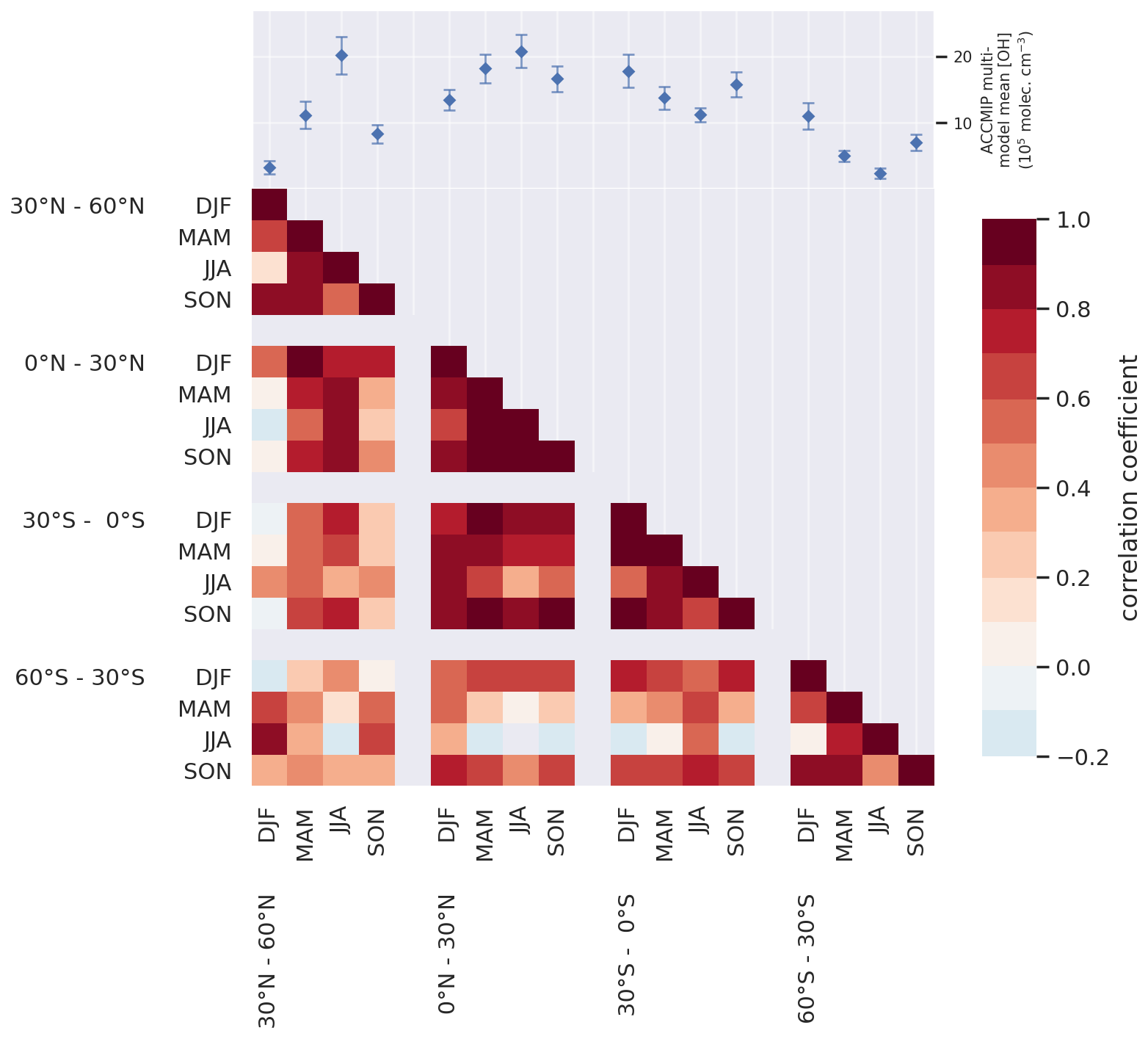
Figure 3 Error correlations for model OH concentrations in different latitude bands and seasons (denoted as R_A,AM in the text). Pearson's error correlation coefficients are calculated for the ensemble of 11 different ACCMIP models. The mean and standard deviation of the ACCMIP ensemble for each latitude and season is inset above.

We replicate the 16 × 16 spatial and seasonal OH error covariance matrix S_A,AM constructed from the ACCMIP data to create a 48 × 48 error covariance matrix for the 3 years of our analysis, resulting in the following block matrix:

$$\begin{array}{}\text{(11)}& \left[\begin{array}{ccc}{\mathbf{S}}_{\mathrm{A},\mathrm{AM}}& {\mathbf{S}}_{\mathrm{A},\mathrm{AM}}& {\mathbf{S}}_{\mathrm{A},\mathrm{AM}}\\ {\mathbf{S}}_{\mathrm{A},\mathrm{AM}}& {\mathbf{S}}_{\mathrm{A},\mathrm{AM}}& {\mathbf{S}}_{\mathrm{A},\mathrm{AM}}\\ {\mathbf{S}}_{\mathrm{A},\mathrm{AM}}& {\mathbf{S}}_{\mathrm{A},\mathrm{AM}}& {\mathbf{S}}_{\mathrm{A},\mathrm{AM}}\end{array}\right].\end{array}$$

This matrix is low-rank because it was constructed with information from only 11 models to estimate 48 state vector elements. We use the method of Schäfer and Strimmer (2005) to shrink the off-diagonal errors and produce a matrix that is positive-definite and invertible. Schäfer and Strimmer (2005) show that their method produces a more accurate estimate of the true error covariance matrix (where accuracy is defined by comparison of the true and estimated eigenvalues). After off-diagonal shrinkage, matrices along the diagonal of the block matrix differ from those from off the diagonal. We refer to the resulting 16 × 16 covariance matrices of spatial and seasonal errors within years as ${{\mathbf{S}}_{\mathrm{A},\mathrm{AM}}}^{\prime \prime }$ and between years as ${{\mathbf{S}}_{\mathrm{A},\mathrm{AM}}}^{\prime }$. Additionally, we refer to the error variances of the global-mean $\left[\stackrel{\mathrm{‾}}{\mathrm{OH}}\right]$ for 1 year inferred from these matrices as ${{\mathit{\sigma }}_{\mathrm{AM}}^{\mathrm{2}}}^{\prime \prime }$ and ${{\mathit{\sigma }}_{\mathrm{AM}}^{\mathrm{2}}}^{\prime }$, respectively.

We can then construct S_A,OH from the regularized ACCMIP covariance matrices ${\mathbf{S}}_{\mathrm{A},{\mathrm{AM}}^{\prime \prime }}$ and ${\mathbf{S}}_{\mathrm{A},{\mathrm{AM}}^{\prime }}$ scaled by the annual-mean error variances inferred from the MCF observations ${\mathit{\sigma }}_{ij}^{\mathrm{2}}$ (Eq. 10) and the spatial and seasonal error variances inferred from the ACCMIP model ${{\mathit{\sigma }}_{\mathrm{AM}}^{\mathrm{2}}}^{\prime \prime }$ and ${{\mathit{\sigma }}_{\mathrm{AM}}^{\mathrm{2}}}^{\prime }$. We can formulate S_A, OH as a block matrix, where each block is an appropriately scaled ACCMIP covariance matrix for 1 year, as follows:

$$\begin{array}{}\text{(12)}& \begin{array}{rl}& {\mathbf{S}}_{\mathrm{A},\mathrm{OH}}\\ & =\left[\begin{array}{ccc}\frac{{\mathit{\sigma }}_{\mathrm{11}}^{\mathrm{2}}}{{{\mathit{\sigma }}_{\mathrm{AM}}^{\mathrm{2}}}^{\prime \prime }}{{\mathbf{S}}_{\mathrm{A},\mathrm{AM}}}^{\prime \prime }& \frac{{\mathit{\sigma }}_{\mathrm{12}}^{\mathrm{2}}}{{{\mathit{\sigma }}_{\mathrm{AM}}^{\mathrm{2}}}^{\prime }}{{\mathbf{S}}_{\mathrm{A},\mathrm{AM}}}^{\prime }& \frac{{\mathit{\sigma }}_{\mathrm{13}}^{\mathrm{2}}}{{{\mathit{\sigma }}_{\mathrm{AM}}^{\mathrm{2}}}^{\prime }}{{\mathbf{S}}_{\mathrm{A},\mathrm{AM}}}^{\prime }\\ \frac{{\mathit{\sigma }}_{\mathrm{21}}^{\mathrm{2}}}{{{\mathit{\sigma }}_{\mathrm{AM}}^{\mathrm{2}}}^{\prime }}{{\mathbf{S}}_{\mathrm{A},\mathrm{AM}}}^{\prime }& \frac{{\mathit{\sigma }}_{\mathrm{22}}^{\mathrm{2}}}{{{\mathit{\sigma }}_{\mathrm{AM}}^{\mathrm{2}}}^{\prime \prime }}{{\mathbf{S}}_{\mathrm{A},\mathrm{AM}}}^{\prime \prime }& \frac{{\mathit{\sigma }}_{\mathrm{23}}^{\mathrm{2}}}{{{\mathit{\sigma }}_{\mathrm{AM}}^{\mathrm{2}}}^{\prime }}{{\mathbf{S}}_{\mathrm{A},\mathrm{AM}}}^{\prime }\\ \frac{{\mathit{\sigma }}_{\mathrm{31}}^{\mathrm{2}}}{{{\mathit{\sigma }}_{\mathrm{AM}}^{\mathrm{2}}}^{\prime }}{{\mathbf{S}}_{\mathrm{A},\mathrm{AM}}}^{\prime }& \frac{{\mathit{\sigma }}_{\mathrm{32}}^{\mathrm{2}}}{{{\mathit{\sigma }}_{\mathrm{AM}}^{\mathrm{2}}}^{\prime }}{{\mathbf{S}}_{\mathrm{A},\mathrm{AM}}}^{\prime }& \frac{{\mathit{\sigma }}_{\mathrm{33}}^{\mathrm{2}}}{{{\mathit{\sigma }}_{\mathrm{AM}}^{\mathrm{2}}}^{\prime \prime }}{{\mathbf{S}}_{\mathrm{A},\mathrm{AM}}}^{\prime \prime }\end{array}\right]\end{array}.\end{array}$$

This enforces error variances and covariances for annual global-mean OH concentrations identical to the values ${\mathit{\sigma }}_{ij}^{\mathrm{2}}$ from Eq. (10).

We refer to Eq. (12) as the full-correlation error covariance matrix. We will also test the effect of simpler OH correlation assumptions on inversion results while keeping the state vector the same. First is a no-correlation diagonal error covariance matrix that assumes no error correlation between years, seasons, or latitude bands. Second is a correlated-years error covariance matrix that includes error correlations between years but with no spatial or seasonal structure. We scale the correlated-years error covariance matrix such that the error (co)variances for $\left[\stackrel{\mathrm{‾}}{\mathrm{OH}}\right]$ are identical to ${\stackrel{\mathrm{‾}}{\mathbf{S}}}_{\mathrm{A},\mathrm{OH}}$ in Eq. (10). We cannot do the same for the no-correlation error covariance matrix because it is diagonal; however, we scale it such that the error variance of the 3-year average is identical to that represented by ${\stackrel{\mathrm{‾}}{\mathbf{S}}}_{\mathrm{A},\mathrm{OH}}$. The variance of the 3-year average is therefore identical for all three error covariance matrices.

4 Results and discussion

4.1 Quantifying emissions

Figure 4 compares the global-mean dry-column mixing ratio ($X_{{\mathrm{CH}}_{\mathrm{4}}}$) simulated by GEOS-Chem and observed by GOSAT and AIRS. The prior simulation shows an increasing negative bias with time because of an incorrect balance between methane sources and sinks. All inversions (posterior solutions) are successful in correcting this bias, including its seasonality.

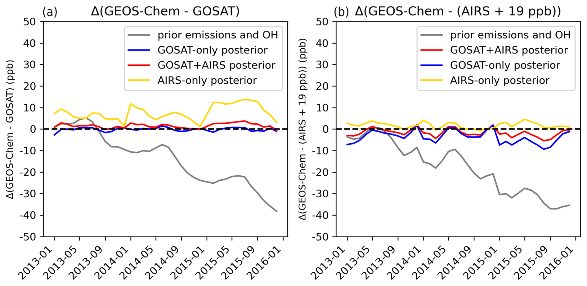
Figure 4 Difference between the global-mean dry-column mixing ratio ($X_{{\mathrm{CH}}_{\mathrm{4}}}$) simulated by GEOS-Chem and observed by GOSAT (a) and AIRS (b). Monthly mean results are shown for the 2013–2015 inversion period. The GEOS-Chem simulation is driven by either prior or posterior values for emissions and OH concentrations. Posterior values are from inversions using either GOSAT or AIRS observations or both. The 19 ppb correction applied to AIRS observations is to remove the bias with GOSAT (Sect. 2.1).

The inversions optimize both methane emissions and OH concentrations. Figure 5 shows the prior non-wetland emissions and 2013–2015 posterior-to-prior correction factors for all three inversions, as well as the averaging kernel sensitivities. The GOSAT-only inversion (Fig. 5b) shows upward corrections to the southern United States, Brazil, and eastern Africa and downward corrections to East Asia and parts of Russia, consistent with Zhang et al. (2021), who used similar prior estimates. The AIRS-only inversion shows generally similar results but weaker averaging kernel sensitivities. Results from the AIRS-only inversion are consistent with those of the GOSAT-only inversion, with the exception of strong upward corrections over Brazil, Argentina, and India, which together cause much higher global methane emissions in the AIRS-only solution than the two solutions constrained by GOSAT observations. The greater power of the GOSAT data to constrain emissions on the 4° × 5° grid is measured by the DOFS (144 for GOSAT, 33 for AIRS). Adding AIRS observations to GOSAT increases the DOFS by only 4 %, indicating that the information on emissions from these two sensors has extensive overlap. The GOSAT +A IRS inversion results largely follow those of the GOSAT-only inversion, but the global posterior emission estimate is lower than in either the GOSAT-only or AIRS-only inversions because of selected regions where AIRS has influence, such as to decrease emissions in China.

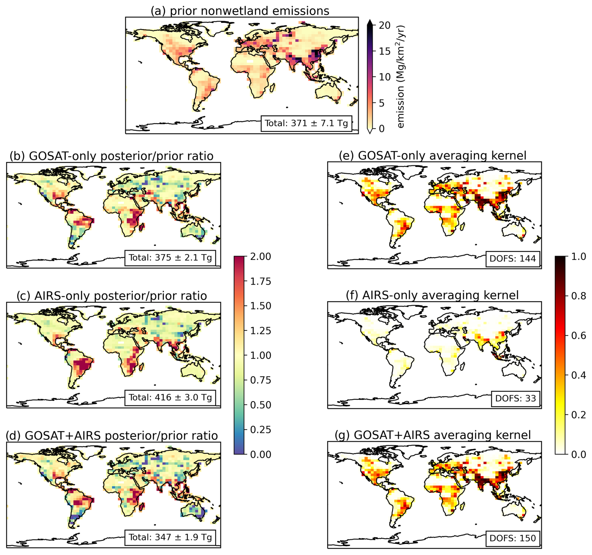
Figure 5 Optimized global distributions of 2013–2015 non-wetland methane emissions using GOSAT, AIRS, and GOSAT + AIRS observations. Prior emissions are shown in (a). The average posterior-to-prior ratios from 2013–2015 for inversions with each set of observations are shown in (b)–(d). Total emissions are inset in (a)–(d) with their error standard deviations. Averaging kernel sensitivities (diagonal elements of the averaging kernel matrix) averaged over 2013–2015 are shown in (e)–(g). The averaging kernel sensitivities represent the ability of the inversion to constrain the posterior solution independently of the prior estimate (1 = fully, 0 = not at all). The degrees of freedom for signal (DOFS) for the 1009 total 4° × 5° grid cells averaged over 3 years are inset.

Our finding that AIRS does not add much information for optimizing methane emissions beyond GOSAT alone is not inconsistent with a previous finding by Worden et al. (2015) that TIR information from the TES satellite instrument improves the retrieval of lower tropospheric methane compared to a GOSAT-only retrieval. In our inversion, the GEOS-Chem forward model effectively provides the information to separate lower tropospheric methane from higher altitudes. An implication is that TIR observations are not necessary for enforcing that separation beyond the information from GEOS-Chem.

We find small (< 10 Tg a⁻¹) changes from year to year for methane emissions in all solutions, and most of these changes are attributed to non-wetland emissions. This is consistent with the solutions in Yin et al. (2021), who find global methane emission changes over 2013–2015 on the order of 1 %–2 %.

Figure 6 shows inversion results for the seasonality of wetland emissions in the 14 subcontinental regions of the WetCHARTs inventory used as a prior estimate. The seasonality and magnitude of the GOSAT and GOSAT + AIRS posterior estimates are consistent with Zhang et al. (2021), who used a similar wetland state vector but with more years of GOSAT data. Our posterior produces negative emissions in eastern Canada in the spring, and this feature is also present in the solution of Zhang et al. (2021). They attribute these negative emissions to potential soil sinks in the region. Remarkably, the AIRS-only inversion shows the same feature. Even though the prior simulation is biased low (Fig. 4), the posterior global sum of non-wetland and wetland emissions in the GOSAT and GOSAT + AIRS inversions is lower than the prior estimate. This is because of a compensating decrease in $\left[\stackrel{\mathrm{‾}}{\mathrm{OH}}\right]$, as analyzed below.

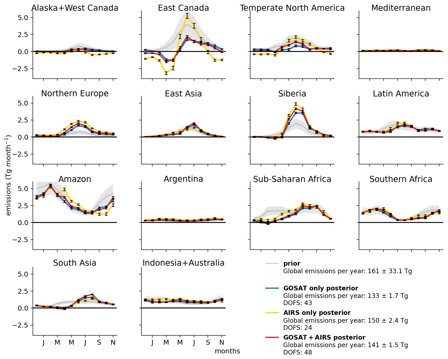
Figure 6 Monthly mean 2013–2015 wetland emissions for the 14 WetCHARTs subcontinental regions as defined by Bloom et al. (2017). Prior emission estimates from the mean of the WetCHARTs inventory ensemble are compared to posterior emissions from the GOSAT, AIRS, and GOSAT + AIRS inversions. The degrees of freedom (DOFS) for signal aggregated to 14 regions × 12 months = 168 state vector elements are also given.

4.2 Quantifying global-mean OH concentrations independently of emissions

We now turn our attention to the ability of the satellite observations to constrain the global annual-mean OH concentration, $\left[\stackrel{\mathrm{‾}}{\mathrm{OH}}\right]$, independently of emissions and for individual years. Let E denote the global annual-mean methane emission rate. The annual rate of change in atmospheric methane mass, $\mathrm{\Delta }m/\mathrm{\Delta }t$, is given by

$$\begin{array}{}\text{(13)}& {\displaystyle \frac{\mathrm{\Delta }m}{\mathrm{\Delta }t}}=E-k\left[\stackrel{\mathrm{‾}}{\mathrm{OH}}\right]m-L,\end{array}$$

where k is the rate constant for oxidation of methane by tropospheric OH with a suitable temperature kernel (Prather and Spivakovsky, 1990) and L is the sum of other minor sinks with $L\ll k\left[\stackrel{\mathrm{‾}}{\mathrm{OH}}\right]m$. Considering that $\mathrm{\Delta }m/\mathrm{\Delta }t$ is set by the observations used in the inversion and that L is minor and not optimized, we see that corrections to E and $\left[\stackrel{\mathrm{‾}}{\mathrm{OH}}\right]$ are necessarily correlated. In order to constrain $\left[\stackrel{\mathrm{‾}}{\mathrm{OH}}\right]$, we need independent information on emissions. The lower-atmosphere gradients over land observed by GOSAT can provide that information, as pointed out by Zhang et al. (2021) and shown in Sect. 4.1, but the AIRS TIR measurements cannot, and this is reflected in the low DOFS of Figs. 5 and 6.

Figure 7 shows the corrections to E and $\left[\stackrel{\mathrm{‾}}{\mathrm{OH}}\right]$ for individual years from the inversions. The inversions apply a systematic correction to $\left[\stackrel{\mathrm{‾}}{\mathrm{OH}}\right]$ in all 3 years, reflecting bias in the prior [OH] and a smaller interannual variability. The AIRS-only inversion has excessive $\left[\stackrel{\mathrm{‾}}{\mathrm{OH}}\right]$, despite its high DOFS for OH, to offset its poorly constrained and excessive global emission (Fig. 5). Figure 7b shows the rows of the reduced averaging kernel matrix summing emissions globally (Eq. 8) and diagnoses the ability of the inversion to separately correct $\left[\stackrel{\mathrm{‾}}{\mathrm{OH}}\right]$ and E in individual years. We find that the averaging kernels for $\left[\stackrel{\mathrm{‾}}{\mathrm{OH}}\right]$ in individual years are strongly peaked, with no significant aliasing from emissions and only minor aliasing with $\left[\stackrel{\mathrm{‾}}{\mathrm{OH}}\right]$ for other years. We conclude that $\left[\stackrel{\mathrm{‾}}{\mathrm{OH}}\right]$ can be optimized for individual years and independently of emissions. Some smoothing of the inverse solution to $\left[\stackrel{\mathrm{‾}}{\mathrm{OH}}\right]$ across years is to be expected in view of the long lifetime of methane, but we are still able to capture individual years and thus interannual variability of $\left[\stackrel{\mathrm{‾}}{\mathrm{OH}}\right]$. AIRS alone is able to separate $\left[\stackrel{\mathrm{‾}}{\mathrm{OH}}\right]$ from emissions, but as mentioned above the bias in its optimization of emissions propagates to a bias in its optimization of $\left[\stackrel{\mathrm{‾}}{\mathrm{OH}}\right]$. GOSAT + AIRS provides only slightly more information than GOSAT alone. A similar averaging kernel analysis by Maasakkers et al. (2019) for 2010–2015 GOSAT observations found that the observations could constrain the average $\left[\stackrel{\mathrm{‾}}{\mathrm{OH}}\right]$ over all years but not the interannual variability. In that study the emission trend was imposed to be linear, which would strongly detract from the ability to independently constrain interannual variability of $\left[\stackrel{\mathrm{‾}}{\mathrm{OH}}\right]$.

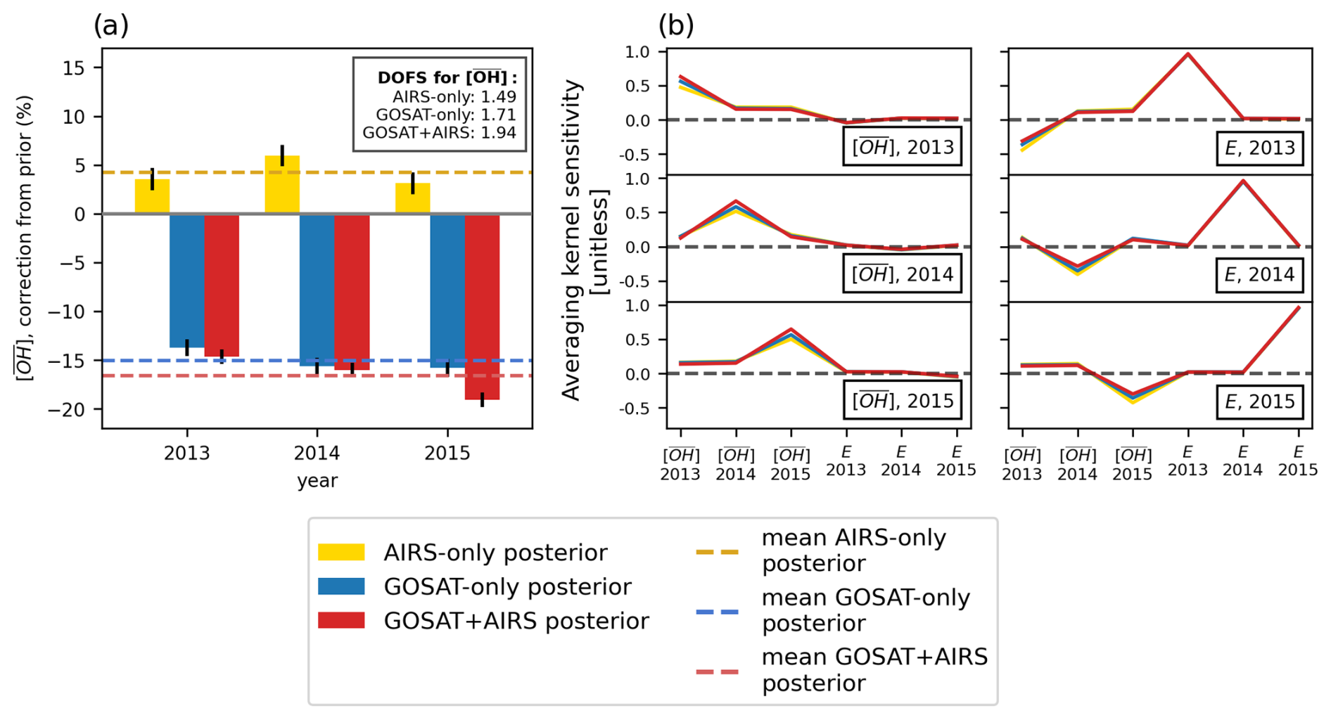
Figure 7 Ability of inversions of GOSAT, AIRS, and GOSAT + AIRS methane observations to quantify global annual-mean tropospheric $\left[\stackrel{\mathrm{‾}}{\mathrm{OH}}\right]$ for individual years and independently of emissions. (a) The 2013–2015 percentage corrections to the $\left[\stackrel{\mathrm{‾}}{\mathrm{OH}}\right]$ prior estimate. Posterior error standard deviations are shown as error bars. DOFS are shown in the inset (DOFS = 3 would imply perfect separate quantification of $\left[\stackrel{\mathrm{‾}}{\mathrm{OH}}\right]$ in individual years). (b) Rows of the reduced averaging kernel matrix describing the ability of the observing system to separately quantify emissions (E) and $\left[\stackrel{\mathrm{‾}}{\mathrm{OH}}\right]$ for the individual years. A perfect observing system would have an averaging kernel sensitivity of 1 for the reduced state vector element of interest (perfect characterization) and 0 for other elements (no sensitivity of the solution to other elements).

Our finding that AIRS provides little information on $\left[\stackrel{\mathrm{‾}}{\mathrm{OH}}\right]$ beyond that provided by GOSAT contrasts with the Zhang et al. (2018) OSSE that found TIR methane observations to add significant information on emissions and $\left[\stackrel{\mathrm{‾}}{\mathrm{OH}}\right]$ relative to SWIR alone. That OSSE may have found a greater benefit from TIR because they assumed the SWIR and TIR synthetic observations to be perfectly consistent, while there are likely inconsistencies between the GOSAT and AIRS observations beyond our global correction (Fig. 1) that translate into the differences between GOSAT-only and AIRS-only inversion results. Zhang et al. (2018) also gave the same weight to SWIR and TIR observations, whereas we find that the weight for AIRS observations should be half of that for GOSAT based on optimization of the γ coefficients (Sect. 2.5). Beyond this, comparison of our results with Zhang et al. (2018) is difficult because they emulated different satellite instruments (TROPOMI for SWIR and CrIS for TIR) and did not report their assumed observational error variances.

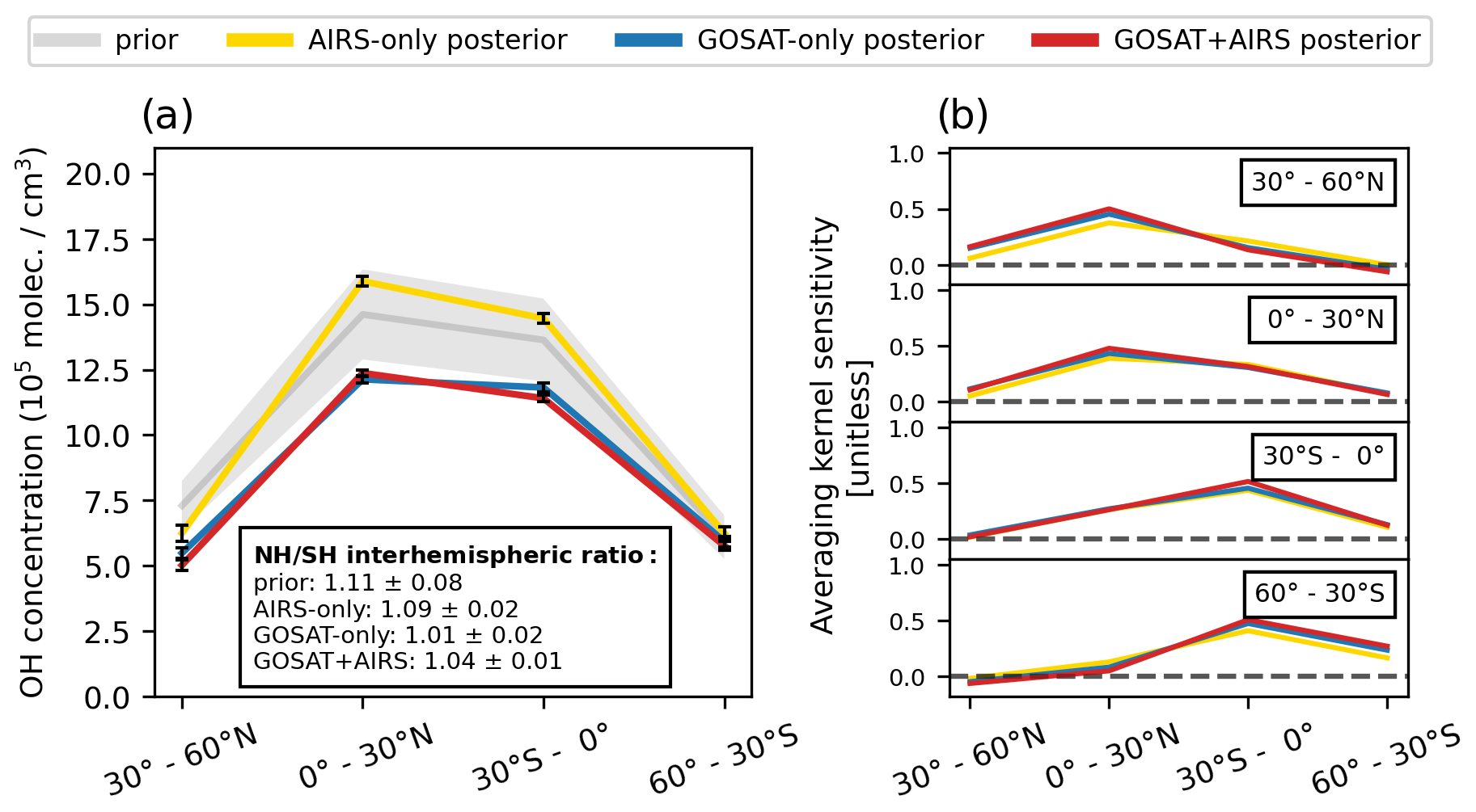
Figure 8 Ability of inversions of GOSAT, AIRS, and GOSAT + AIRS methane observations to resolve the latitudinal variability of OH concentrations. (a) Latitudinal distribution of mass-weighted tropospheric [OH] in the prior estimate (prior error standard deviation is shown with shading) and in the posterior estimates. The $\mathrm{NH}/\mathrm{SH}$ interhemispheric ratio and its error standard deviation are inset. (b) Rows of the reduced averaging kernel matrix describing the ability of the observing system to separately quantify [OH] in different latitudinal bands. A perfect observing system would have an averaging kernel sensitivity of 1 for the reduced state vector element of interest (perfect characterization) and 0 for other elements (no error correlation).

4.3 Resolving spatial and seasonal patterns in OH concentrations

We now investigate the ability of the methane observations to constrain the spatial and seasonal variations in OH concentrations. Figure 8 shows the corrections to OH concentrations from the inversion as a function of latitude and the corresponding rows of the averaging kernel matrix. We find that GOSAT and GOSAT + AIRS provide only weak constraints on the OH latitudinal distribution because prior errors from the ACCMIP ensemble are highly correlated (Fig. 3). We are unable to resolve the midlatitudes, where averaging kernel rows show higher sensitivity to the adjacent tropical latitude band and almost no sensitivity to the midlatitudes themselves. There is some information on the interhemispheric ratio of OH concentrations, with the inversion decreasing the $\mathrm{NH}/\mathrm{SH}$ ratio from 1.11 ± 0.08 in the prior estimate to 1.01 ± 0.02 (for GOSAT) and 1.04 ± 0.01 (for GOSAT + AIRS). This is consistent with previous inversions of methane observations showing downward corrections in the $\mathrm{NH}/\mathrm{SH}$ ratio (Zhang et al., 2021) and independent evidence from MCF observations that current model $\mathrm{NH}/\mathrm{SH}$ ratios are too high (Naik et al., 2013; Patra et al., 2014). Nevertheless, we see from the averaging kernels that there is significant aliasing of the information between the northern and southern tropics because errors are highly correlated across models (Fig. 3). It could be that the ensemble of ACCMIP models exaggerates the error correlation on account of using the same anthropogenic emissions, but OH in the tropics is more sensitive to lightning, fires, and clouds, which vary across the models.

The seasonal cycle for [OH] is shown in Fig. 9. We find from the averaging kernel matrix that the inversion provides significant information on the seasonality of [OH] in the two hemispheres, despite the smearing across latitudinal bands found in Fig. 8. There is some aliasing between adjacent seasons, but winter and summer are well separated; however, this is mainly the case for the tropics since there is little information from midlatitudes (Fig. 8). The GOSAT + AIRS inversion increases the amplitude of the seasonal cycle in both hemispheres. The posterior seasonal patterns from the GOSAT and GOSAT + AIRS inversions do not differ significantly from the prior estimates and thus support the prior estimates.

Figure 9 The same as Fig. 8 but for the seasonality of OH concentrations in each hemisphere.

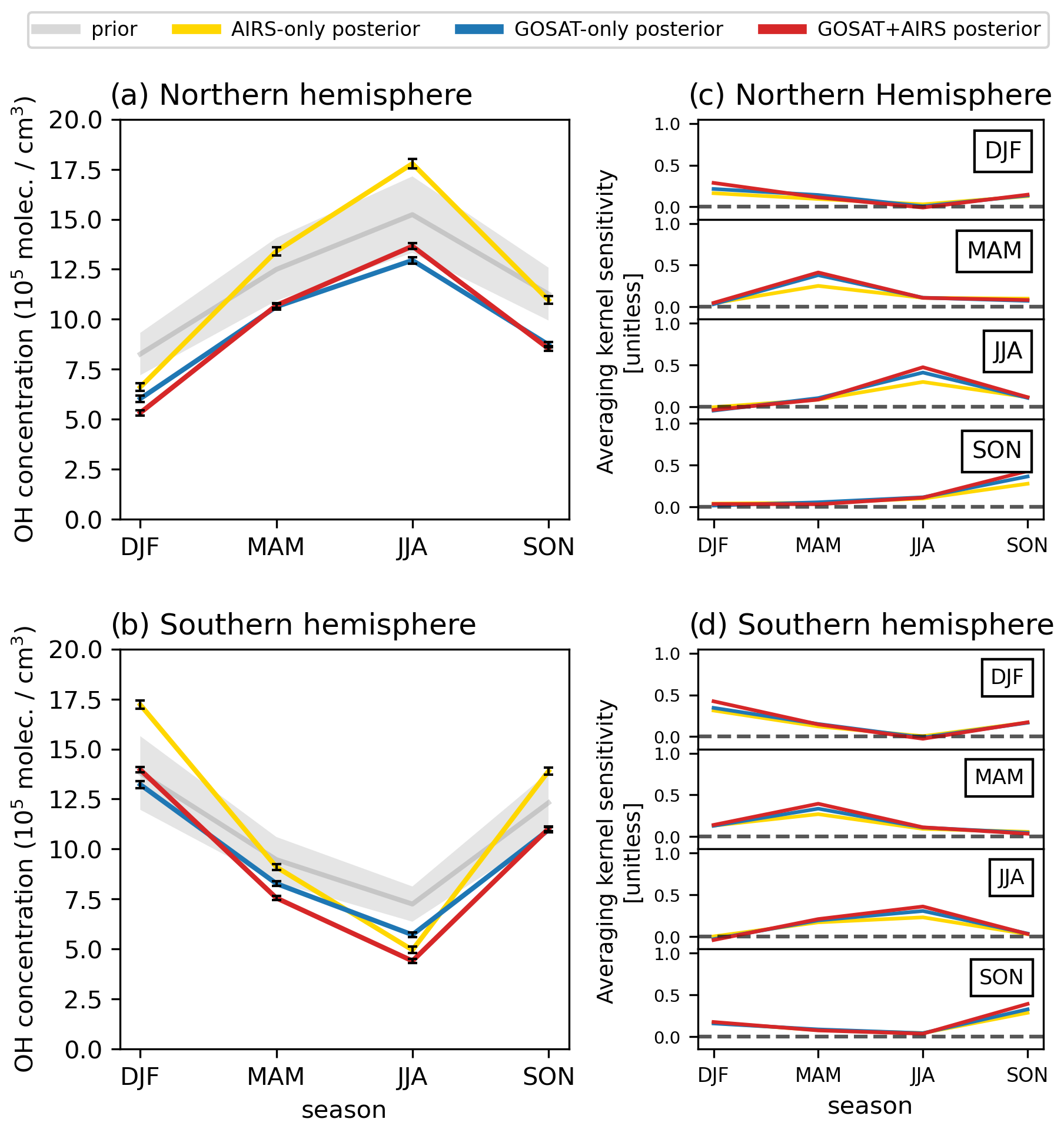
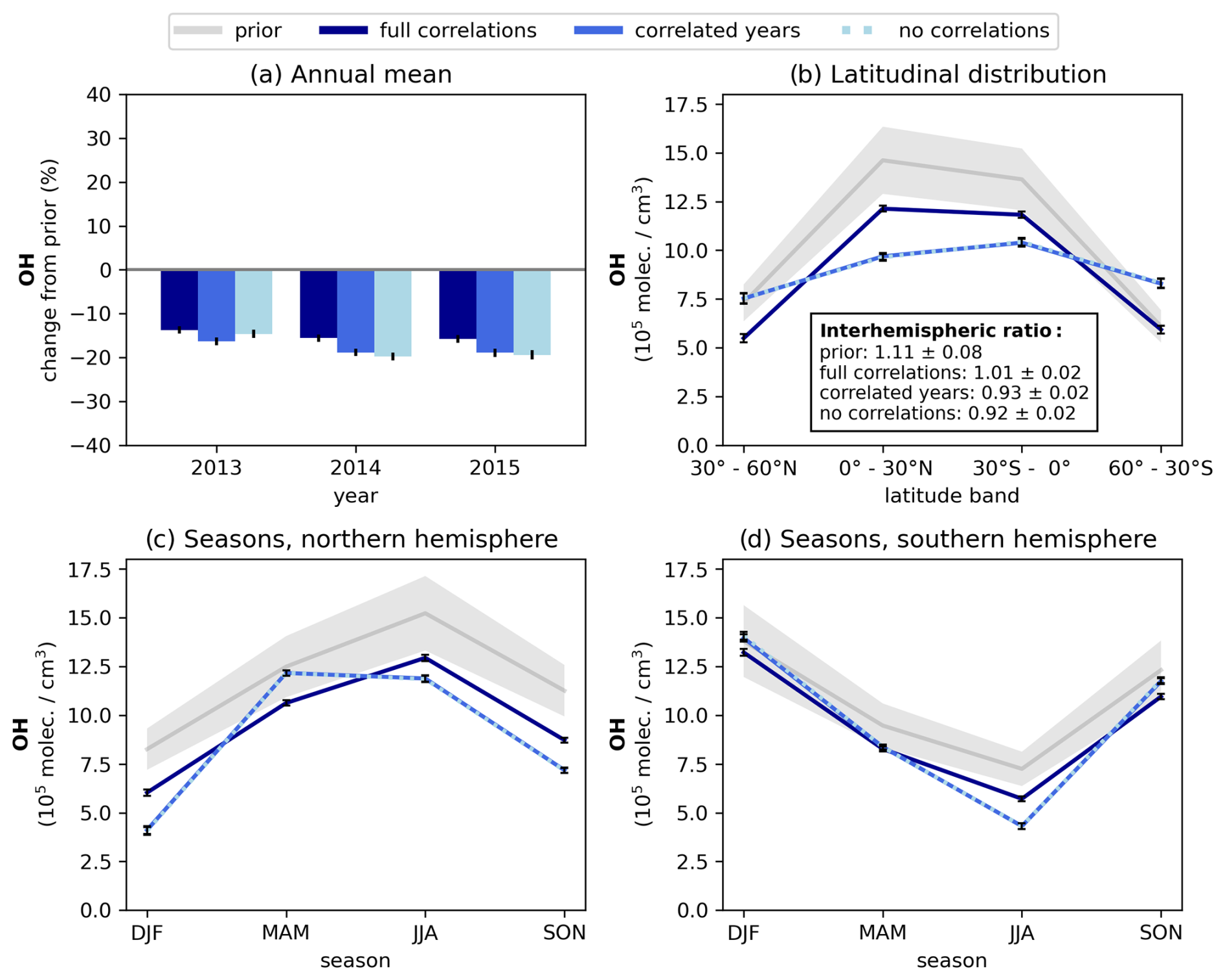
Figure 10 Sensitivity of [OH] inversion results to the prior error correlations imposed for interannual, seasonal, and latitudinal variability. Results are shown for the 2013–2015 GOSAT-only inversion, for our base inversion with full error correlations from the ACCMIP ensemble (same results as in Figs. 7–9), and for inversions with no [OH] error correlations or with [OH] error correlations for individual years only. Panels show (a) annual-mean $\left[\stackrel{\mathrm{‾}}{\mathrm{OH}}\right]$ for individual years, (b) 2013–2015 latitudinal distribution, and (c, d) 2013–2015 seasonal variations for the Northern Hemisphere and Southern Hemisphere. Prior error standard deviations are shown with shading. The correlated-years and no-correlation inversions show the same latitudinal and seasonal variations in [OH].

We have found that the ability of the inversion to optimize spatial and temporal features of the OH distribution is limited by prior error correlations from the independent knowledge expressed by the ACCMIP models. We now examine the effect of these prior error correlations in sensitivity simulations for GOSAT-only inversions in which we either assume no error correlations between OH state vector elements (no-correlation inversion) or error correlations only for the interannual variability of $\left[\stackrel{\mathrm{‾}}{\mathrm{OH}}\right]$ (correlated-years inversion), as described by Eq. (10). Aggregated errors in $\left[\stackrel{\mathrm{‾}}{\mathrm{OH}}\right]$ are scaled to be the same in all inversions, as described in Sect. 3. Figure 10 shows the results for the GOSAT-only inversion. Constraints on $\left[\stackrel{\mathrm{‾}}{\mathrm{OH}}\right]$ are similar across all inversions, as would be expected since our base full-correlation inversion can effectively constrain that quantity for individual years. The inversions without error correlations show larger perturbations in the latitudinal distribution of [OH], with higher values at midlatitudes, lower values in the tropics, and a greater shift to the Southern Hemisphere. The spatial error correlations imposed by the ACCMIP models (Fig. 3) suppress these changes in the base inversion. To the extent that the ACCMIP ensemble fairly represents error correlations in the OH distribution, ignoring that prior information would result in overfit to observations. The seasonality in each hemisphere is better constrained by the observing system because there is more contrast between summer and winter, with the northern and southern tropics being opposites in the seasonal phase. However, we find that ignoring seasonal error correlations in the no-correlation and correlated-years inversions results in opposite corrections to OH concentrations in spring and summer of the Northern Hemisphere that are in fact highly correlated in the ACCMIP models (Fig. 3).

5 Conclusions

We examined the ability of satellite observations of atmospheric methane to quantify different features of the tropospheric OH distribution including global multi-year mean, interannual variability in the global mean, interhemispheric ratio, intra-hemispheric latitudinal variation, and seasonality. The work was motivated by the need to find a replacement proxy for tropospheric OH as methyl chloroform (MCF) concentrations fall below detectable levels and to explore how much information can be extracted from the satellite observations.

For this purpose we used a 3-year (2013–2015) analytical inversion of GOSAT (SWIR) and AIRS (TIR) satellite observations. SWIR observations have near-unit sensitivity for the whole atmospheric column but are limited to daytime and (mainly) land. TIR observations are sensitive mainly to the middle and upper troposphere but include nighttime and oceans.

Several previous inversions investigated the ability of satellite observations of methane to quantify the OH distribution but did not properly account for prior error correlations in that distribution. Here we provide detailed accounting of this error correlation, including for global-mean OH and interannual variability using MCF and for spatial and seasonal variations using the ACCMIP ensemble of 11 global atmospheric chemistry models. We find strong prior error correlations between latitude bands and seasons.

Optimizing OH concentrations from satellite observations of methane requires independent information on emissions, and the SWIR observations are essential for that purpose. We find that a GOSAT-only inversion can effectively constrain global-mean OH and its interannual variability independently of emissions, thus providing information comparable to MCF. Adding AIRS observations to the inversion does not significantly improve the constraint. Retrievals combining SWIR and TIR information from the same instrument, such as GOSAT-2 (Kuze et al., 2022; Suto, 2022), could possibly improve the constraint by being internally consistent. This would need to be examined in future work. We conducted the inversion for only 3 years (2013–2015) to demonstrate the capability for constraining OH interannual variability. Qu et al. (2024) recently conducted an inversion of the full GOSAT record from 2011 to 2022 to quantify the OH interannual variability over that 13-year period.

The ability of the inversion to resolve the latitudinal variability of OH is very limited because of strong error correlation across latitudes in the ACCMIP ensemble. Not accounting for this error correlation would result in an overfit to observations. In particular, there is no information on OH at midlatitudes in particular. The inversion provides some information on the interhemispheric OH ratio, and this is important for interpreting the corresponding gradient in methane observations (East et al., 2024). There is also some information on seasonality of OH concentrations, and the inversion confirms the prior seasonality from the ACCMIP models.

Acquiring finer regional-scale information on OH is of great interest, but the long lifetime of methane likely limits the information that it can provide to the global scale, even with improved satellite instruments. Satellite observations of shorter-lived species driving OH chemistry including H₂O, O₃, CO, NO₂, and HCHO provide fine-scale information on OH through chemical data assimilation (Miyazaki et al., 2020), but the results may be biased by errors in the chemical mechanisms (Travis et al., 2020; Shah et al., 2023). The global-scale information on OH concentrations available from methane observations can be used for independent evaluation of such data assimilation products.