Anthropogenic emission controls reduce summertime ozone–temperature sensitivity in the United States

Ozone–temperature sensitivity is widely used to infer the impact of future climate warming on ozone. However, trends in ozone–temperature sensitivity and possible drivers have remained unclear. Here, we show that the observed summertime surface ozone–temperature sensitivity, defined as the slope of the best-fit line of daily anomalies in ozone versus maximum temperature ($m_{\mathrm{\Delta }{\mathrm{O}}_{\mathrm{3}}-\mathrm{\Delta }{T}_{\text{max}}}$), has decreased by 50 % during 1990–2021 in the continental United States (CONUS), with a mean decreasing rate of −0.57 ppbv K⁻¹ per decade (p < 0.01) across 608 monitoring sites. We conduct high-resolution GEOS-Chem simulations in 1995–2017 to interpret the $m_{\mathrm{\Delta }{\mathrm{O}}_{\mathrm{3}}-\mathrm{\Delta }{T}_{\text{max}}}$ trends and underlying mechanisms in the CONUS. The simulations identify the dominant role of anthropogenic nitrogen oxide (NO_x) emission reduction in the observed $m_{\mathrm{\Delta }{\mathrm{O}}_{\mathrm{3}}-\mathrm{\Delta }{T}_{\text{max}}}$ decrease. We find that approximately 76 % of the simulated decline in $m_{\mathrm{\Delta }{\mathrm{O}}_{\mathrm{3}}-\mathrm{\Delta }{T}_{\text{max}}}$ can be attributed to the temperature indirect effects arising from the shared collinearity of other meteorological effects (such as humidity, ventilation, and transport) on ozone. The remaining portion (24 %) is mostly due to the temperature direct effects, in particular four explicit temperature-dependent processes, including biogenic volatile organic compound (BVOC) emissions, soil NO_x emissions, dry deposition, and thermal decomposition of peroxyacetyl nitrate (PAN). With reduced anthropogenic NO_x emissions, the expected ozone enhancement from temperature-driven BVOC emissions, dry deposition, and PAN decomposition decreases, contributing to the decline in $m_{\mathrm{\Delta }{\mathrm{O}}_{\mathrm{3}}-\mathrm{\Delta }{T}_{\text{max}}}$. However, soil NO_x emissions increase $m_{\mathrm{\Delta }{\mathrm{O}}_{\mathrm{3}}-\mathrm{\Delta }{T}_{\text{max}}}$ with anthropogenic NO_x emission reduction, indicating an increasing role of soil NO_x emissions in shaping the ozone–temperature sensitivity. As indicated by the decreased $m_{\mathrm{\Delta }{\mathrm{O}}_{\mathrm{3}}-\mathrm{\Delta }{T}_{\text{max}}}$, model simulations estimate that reduced anthropogenic NO_x emissions from 1995 to 2017 have lowered ozone enhancement from low to high temperatures by 6.8 ppbv averaged over the CONUS, significantly reducing the risk of extreme-ozone-pollution events under high temperatures. Our study illustrates the dependency of ozone–temperature sensitivity on anthropogenic emission levels, which should be considered in future ozone mitigation in a warmer climate.

1 Introduction

Surface ozone harms human health and causes loss of crop yields (Feng et al., 2022; Mills et al., 2018; Monks et al., 2015; Turner et al., 2016; Wang et al., 2024). It is chemically generated from its precursors, including nitrogen oxides (NO_x), volatile organic compounds (VOCs), and carbon monoxide (CO) in the presence of sunlight. The natural sources, chemical kinetics, deposition, and transport of ozone and its precursors are significantly influenced by meteorology and climate (Fiore et al., 2012; Fu and Tian, 2019; Jacob and Winner, 2009; Lu et al., 2019b), shaping the strong sensitivity of surface ozone concentration to meteorological parameters such as temperature. Quantification of ozone–meteorology sensitivity provides a useful tool for predicting daily variation in ozone and for understanding climate–chemistry interactions, yet how anthropogenic emission levels may affect the sensitivity remains unclear. Here, we examine whether long-term anthropogenic control of ozone precursors has changed the response of summertime ozone to daily variations in temperature in the United States (US) and the underlying mechanisms.

High temperature is expected to increase ozone concentrations in polluted environments by boosting biogenic VOCs (BVOCs) and soil NO_x emissions, accelerating photochemical kinetics of ozone formation, and suppressing ozone dry deposition (Hudman et al., 2012; Lin et al., 2020; Porter and Heald, 2019; Pusede et al., 2015; Romer et al., 2018; Varotsos et al., 2019). In addition, temperature-dependent meteorological parameters, such as solar radiation and humidity, and temperature-related meteorological effects, such as air stagnation, ventilation, and regional transport, can also influence the surface ozone level (Kerr et al., 2019; Lu et al., 2019b; Porter and Heald, 2019; Zhang et al., 2022a). Such effects can be reflected in, but at the same time, complicate the ozone–temperature relationship. Still, temperature is often used as a proxy to synthesize the effects of meteorology and climate on ozone. Previous studies have documented a robust positive ozone–temperature sensitivity in NO_x-rich environments, typically defined as the slope of the best-fit line for ozone and temperature ($\mathrm{d}\left[{\mathrm{O}}_{\mathrm{3}}\right]/\mathrm{d}T$), of 2–8 ppbv K⁻¹ across the US, Europe, and China (Bloomer et al., 2009; Gu et al., 2020; Ning et al., 2022; Pusede et al., 2014; Sillman and Samson, 1995; Varotsos et al., 2019). The positive $\mathrm{d}\left[{\mathrm{O}}_{\mathrm{3}}\right]/\mathrm{d}T$ also indicates an ozone climate change penalty; i.e., future warming may deteriorate ozone air quality in the absence of changes in anthropogenic emission activities (Zhang et al., 2022b). The climate penalty requires additional anthropogenic emission reductions to offset the ozone increase in a warmer climate (Wu et al., 2008; Zanis et al., 2022).

While the overall positive ozone–temperature relationship is well recognized, how ozone–temperature sensitivity has changed remains much less explored. Some studies have reported a weakening of regional ozone–temperature sensitivity in California, the midwestern US, and the eastern US based on observations and have suggested reduction in local anthropogenic emissions as a possible driver (Bloomer et al., 2009; Hembeck et al., 2022; Jing et al., 2017; Rasmussen et al., 2013). In contrast, Fu et al. (2015) report large interannual variations in ozone–temperature sensitivity in the southeastern US that may be tied to climate variability. Model simulations project a decrease in ozone–temperature sensitivity in future scenarios with lower anthropogenic emissions in the US (Nolte et al., 2021). These studies indicate that the surface ozone–temperature sensitivity has been shifting, with significant regional variations in the US, yet an up-to-date view on the long-term and continental-scale trends is currently missing. In particular, a quantitative assessment of underlying mechanisms driving long-term changes in surface ozone–temperature sensitivity remains rather unclear, limiting the application of this important metric in predicting future ozone evolution.

In this study, we analyze the present-day (2017–2021) and long-term trends (1990–2021) in the summertime surface ozone–temperature relationship in the continental US (CONUS), combining observational monitoring network and state-of-the-art chemical modeling. We utilize the GEOS-Chem chemical transport model to quantify the role of anthropogenic emission reduction in the long-term trends in ozone–temperature sensitivity and investigate the underlying mechanisms. We also examine the benefit of reduced ozone–temperature sensitivity in ozone mitigation during high temperatures that frequently cause severe ozone pollution extremes.

2 Materials and methods

2.1 Surface ozone measurement in the US

We obtain hourly measurements of surface ozone concentrations from the US Environmental Protection Agency (EPA) Air Quality System (AQS) data program (https://www.epa.gov/aqs, last access: 10 June 2024; US EPA, 2024). Our study period covers 1990–2021, 32 years in total, with a focus on boreal summertime (June, July, August). We derive the daily maximum 8 h average (MDA8) ozone concentrations from the hourly data and select sites with valid summertime ozone measurements for at least 24 years (i.e., ≥ 75 %) in the 1990–2021 period and for at least 3 years in 2017–2021 (Sect. S1 in the Supplement). A total of 608 sites are selected, including 319 urban sites and 289 rural sites (based on EPA categorization). We follow previous studies to categorize the sites into seven geographic areas (Nolte et al., 2021; Rasmussen et al., 2012), including the northwestern US (NWUS), southwestern US (SWUS), northeastern US (NEUS), southeastern US (SEUS), midwestern US (Midwest), mountainous western US (Intermountain West), and central plains of the US (Plains) (Fig. 1).

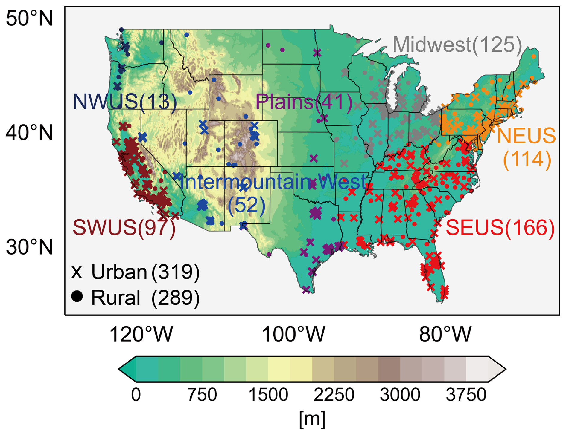
Figure 1 Locations of the 319 urban sites (crosses) and 289 rural sites (dots) across the continental US used in this study. Sites are categorized into seven regions, including the northwestern US (NWUS), southwestern US (SWUS), northeastern US (NEUS), southeastern US (SEUS), midwestern US (Midwest), mountainous western US (Intermountain West), and central plains of the US (Plains). The underlying figure shows terrain elevation.

2.2 Temperature data

The AQS dataset also provides surface temperature measurements that could ideally be used in quantifying the ozone–temperature relationship at individual sites. However, the temperature measurement is largely missing, with only 170 sites (< 30 % of the total 608 sites selected for analysis) providing long-term records (at least 24 years), which is insufficient to support our analysis. Here we use the gridded (0.5° × 0.625°) data of temperature at 2 m above the ground from the Modern-Era Retrospective analysis for Research and Applications version 2 (MERRA-2) dataset (Gelaro et al., 2017), which consistently serves as input for the GEOS-Chem chemical transport model (Sect. 2.4). We align the gridded temperature data with in situ ozone measurement based on the coordinates of individual sites. Evaluation of the MERRA-2 gridded data with in situ measurements of temperature at available sites shows excellent agreement between the two, with a mean bias (MB) of 0.3–1.0 K and a correlation coefficient (r) of 0.96–0.98 for years after 2000; however, the two datasets have slightly larger disparities in the earliest part of our study period (e.g., MB = 0.5 K, r = 0.87 for the year 1990) (Fig. S1 in the Supplement). We also compare temperature trends from MERRA-2 with observations over the period 1990–2021 (Table S1 in the Supplement). While the overall trends are consistent, there are notable overestimations (e.g., NEUS, Plains) and underestimations (e.g., SEUS and SWUS) in different regions, which may lead to biases in interpreting the observed ozone–temperature sensitivity (as observed ozone variation responds to “true” air temperature).

2.3 Definition of ozone–temperature sensitivity

Our goal is to examine the response of summertime MDA8 ozone concentration to the variation in daily maximum temperature (T_max) across the US and the trends in such a response from 1990 to 2021. We use T_max instead of daytime temperature or mean temperature, as strong correlation coefficients between MDA8 ozone and T_max have been revealed in previous studies (e.g., Steiner et al., 2010; Fu et al., 2015). Ozone levels in the US have experienced significant decreasing trends since the 1980s due to anthropogenic emission control measures (Gaudel et al., 2018; Kim et al., 2006; Lin et al., 2017; Simon et al., 2015). The higher ozone concentration in earlier years may obfuscate the long-term trends in ozone–temperature sensitivity if the ozone–temperature sensitivity were derived by the raw measurements. Therefore, we first subtract the monthly-mean MDA8 ozone concentration and T_max from each daily record to derive their daily anomaly (ΔO₃ and ΔT_max) at individual sites for each year. This process allows us to remove the seasonal (monthly) influences and also the 1990–2021 trends in ozone concentration and temperature. We then define the summertime ozone–temperature sensitivity ($m_{\mathrm{\Delta }{\mathrm{O}}_{\mathrm{3}}-\mathrm{\Delta }{T}_{\text{max}}}$) at individual sites as the slope of the best-fit line of daily ΔO₃ versus ΔT_max. Fu et al. (2015) also applied a similar process to quantify ozone–temperature sensitivity across the southeastern US. We calculate the mean values of $m_{\mathrm{\Delta }{\mathrm{O}}_{\mathrm{3}}-\mathrm{\Delta }{T}_{\text{max}}}$ over the sites across the CONUS or individual regions to represent the regional mean ozone–temperature sensitivity. Trends in $m_{\mathrm{\Delta }{\mathrm{O}}_{\mathrm{3}}-\mathrm{\Delta }{T}_{\text{max}}}$ over each site are estimated using the linear regression method, with a 5-year smoothing average applied to the yearly $m_{\mathrm{\Delta }{\mathrm{O}}_{\mathrm{3}}-\mathrm{\Delta }{T}_{\text{max}}}$ to filter the interannual variability. The trends in the mean $m_{\mathrm{\Delta }{\mathrm{O}}_{\mathrm{3}}-\mathrm{\Delta }{T}_{\text{max}}}$ values across the sites are used to represent regional mean trends in the ozone–temperature sensitivity.

2.4 GEOS-Chem model simulation

We use the GEOS-Chem version 11-02-rc chemical transport model (available at http://geos-chem.org, last access: 10 June 2024; Bey et al., 2001) to interpret summertime ozone–temperature sensitivity and its trend in the US. The GEOS-Chem model is driven by MERRA-2 assimilated meteorological data. We conduct simulations over the North America nested-grid domain (10–70° N, 140–40° W) at a horizontal resolution of 0.5° (latitude) × 0.625° (longitude). The global simulations at 2° × 2.5° resolution providing the boundary conditions were configured consistently with the nested simulations (simulation time, chemical schemes, emission inventory, etc.; see discussions below). The GEOS-Chem model describes a state-of-the-art ozone–NO_x–VOC–aerosol–halogen tropospheric chemistry scheme and also includes online calculation of emissions and dry and wet depositions of gases and aerosols. Anthropogenic emissions in this study are from the Community Emissions Data System (CEDS) v_2021_04_21, in which the interannual variability in the US emissions is scaled based on the US National Emissions Inventory (US NEI) (McDuffie et al., 2020). The CEDS inventory indicates a significant decrease in anthropogenic NO_x, non-methane VOC (NMVOC), and CO emissions over the CONUS of 61.7 %, 45.7 %, and 70.7 %, respectively, from 1995–2017.

GEOS-Chem is capable of simulating the temperature's influences on ozone through chemical kinetics, natural emissions, transport, and dry deposition. Chemical kinetics in GEOS-Chem are modularized based on the Jet Propulsion Laboratory (JPL) and the International Union of Pure and Applied Chemistry (IUPAC) scheme (IUPAC, 2013; Sander et al., 2011), with temperature input from the hourly MERRA-2 reanalysis data. GEOS-Chem also includes online calculation of temperature-dependent natural emissions. Biogenic emissions are parameterized following the Model of Emissions of Gases and Aerosols from Nature (MEGAN) version 2.1 algorithm (Guenther et al., 2012), in which biogenic emissions are calculated based on temperature, solar radiation, leaf area index (LAI), and other parameters. Biogenic emissions increase exponentially with temperature, but emissions of some BVOCs are inhibited at higher temperatures. Soil NO_x emissions are calculated based on nitrogen availability in soil, edaphic conditions such as soil temperature and moisture, and other gridded parameters such as vegetation type using the Berkeley–Dalhousie Soil NO_x Parameterization (BDSNP) as described in Hudman et al. (2012). Lightning NO_x emissions are parameterized based on cloud-top heights with the spatial distribution of flash rates constrained by satellite observations (Murray et al., 2012). Biomass burning emissions are from the biomass burning emissions for CMIP6 (BB4CMIP) inventory (van Marle et al., 2017), in which emissions after 1997 are consistent with the Global Fire Emissions Database version 4 (GFED4) inventory (van der Werf et al., 2017). However, temperature's impacts on anthropogenic NO_x and VOC emissions (Liu et al., 2024; Wu et al., 2024) are not considered in our simulation.

Dry deposition of both gas and aerosols is calculated online based on the resistance-in-series algorithm (Wesely, 1989). Surface temperature influences deposition velocity through a stomatal resistance term, which remains low within normal temperatures (e.g., 10–30 °C) but rises at two extremes (below 0 °C and above 40 °C) (Porter and Heald, 2019), contributing to local ozone increases at high temperatures. Wet deposition for water-soluble aerosols and gases in GEOS-Chem is described by Liu et al. (2001) and Amos et al. (2012). NO_x and ozone have low solubility, but wet deposition of NO_x oxidation products may further influence ozone. We do not separately consider temperature's indirect influences on ozone through wet deposition processes in this study.

Table 1 Configurations of model simulations.

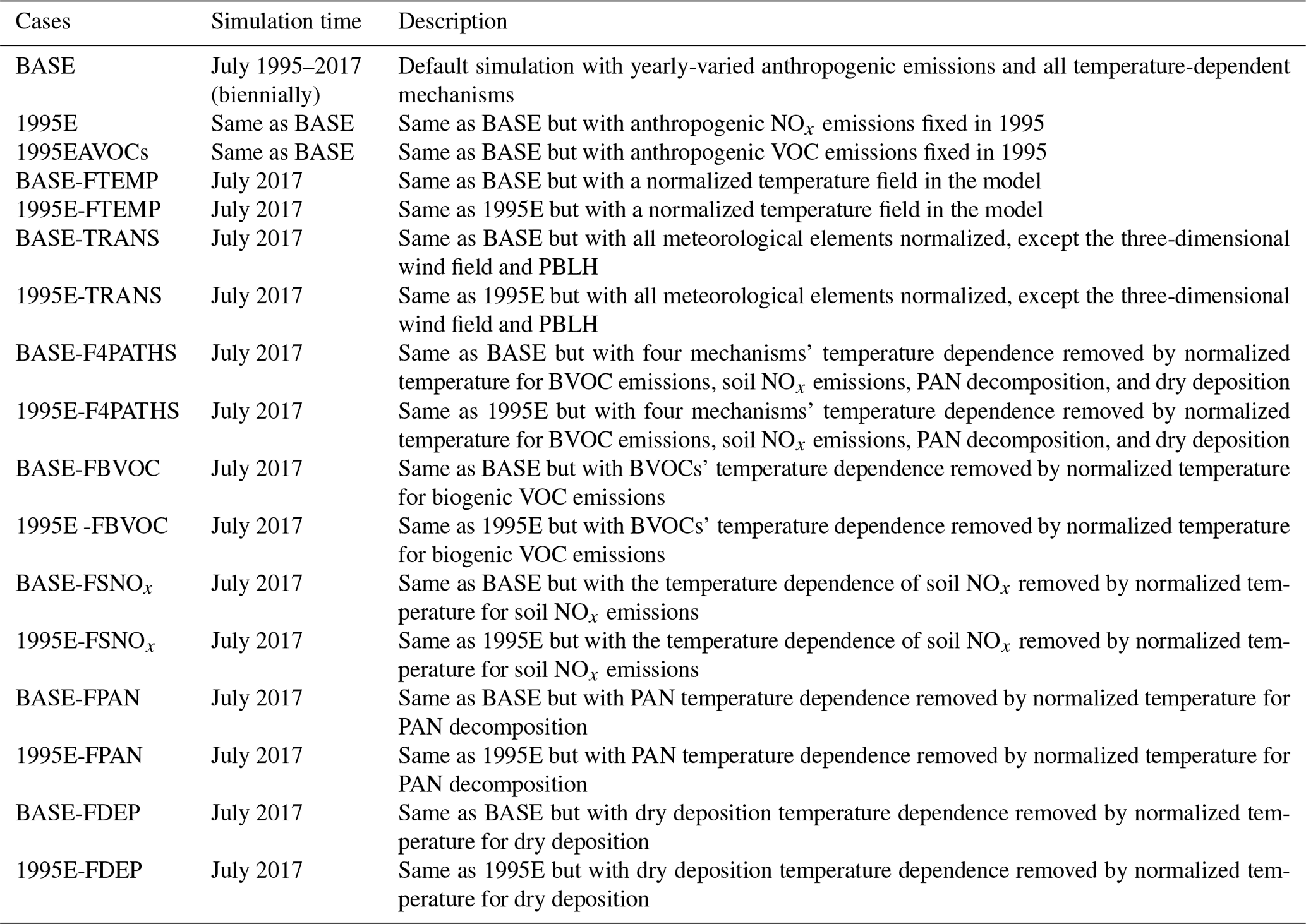
Model simulations are summarized in Table 1. We conduct a BASE simulation for July every 2 years from 1995 to 2017, with a 1-month simulation (June) as model spin-up for both the global and the regional simulations. We do not extend the simulation to earlier or later years due to a lack of a reliable anthropogenic emission inventory by the time this study was designed. The initial chemical fields are close to conditions for July 2005 (the same initial fields used for each set of sensitivity experiments). The 1-month spin-up time can be considered sufficient in this case as the ozone in the urban boundary layer typically has a lifetime ranging from hours to days. However, it may be short for ozone in the free troposphere where ozone has a lifetime of orders of weeks (Monks et al., 2015). To demonstrate this, we conducted an additional set of experiments, starting with a global simulation at 2° × 2.5° resolution from 1 January 2017 to 1 August 2017. The global simulation on 1 June 2017 was then interpolated into the high-resolution nested grid to drive the high-resolution simulation from 1 June 2017 to 1 August 2017. A comparison of surface MDA8 ozone concentrations and ozone–temperature sensitivity between the two sets of simulations is shown in Fig. S2 in the Supplement. We find that the differences between the simulations with 1- and 6-month spin-up times had only minor impacts on ozone concentrations and $m_{\mathrm{\Delta }{\mathrm{O}}_{\mathrm{3}}-\mathrm{\Delta }{T}_{\text{max}}}$. The average differences between the two simulations were only 0.3 % for ozone concentrations and 2.3 % for $m_{\mathrm{\Delta }{\mathrm{O}}_{\mathrm{3}}-\mathrm{\Delta }{T}_{\text{max}}}$, with high spatial consistency (r > 0.99). This confirms that using a 1-month spin-up time for the simulation should not affect the analysis and conclusions. However, for specific regions, more noticeable differences in ozone concentrations and $m_{\mathrm{\Delta }{\mathrm{O}}_{\mathrm{3}}-\mathrm{\Delta }{T}_{\text{max}}}$ exist between the two simulations. A longer spin-up time is favorable for generating global chemical fields when sufficient computational resources are available. The BASE simulation applies the yearly-varied anthropogenic emissions and includes all the abovementioned temperature-dependent mechanisms. We then conduct two simulations for the same 1995–2017 period but in which the domestic anthropogenic NO_x (1995E) or VOC (1995EAVOCs) emissions in the US are fixed to the 1995 level.

We conducted 14 additional sets of sensitivity experiments to explore the role of different mechanisms in the ozone–temperature sensitivity and its trend. First, we separate the effect of temperature on ozone through direct and indirect effects. Here, the temperature direct effect is defined as the effect directly parameterized with temperature in GEOS-Chem, including natural emissions of BVOCs and soil NO_x, chemical kinetics, dry deposition, and other mechanisms that may have minimal impacts on ozone. In comparison, the temperature indirect effect is defined as the effect not directly parameterized with temperature but is also influenced or reflected by temperature, for example humidity, radiation, and transport. The simulation strategy is to remove the daily variation in temperature (while keeping the diurnal cycle) and its influence on ozone daily variations. For this purpose, we generate the mean diurnal cycle of temperature averages over all 31 d in July 2017 at each grid cell. We then feed these normalized temperature data into the calculations of the GEOS-Chem (FTEMP). As such, the FTEMP simulation identifies the indirect effect of temperature on ozone. Comparison of the FTEMP simulation and BASE simulation yields a quantitative assessment of the direct effect.

For the temperature direct effect, we further follow Porter and Heald (2019) to explore the role of four temperature-dependent mechanisms in ozone–temperature sensitivity. These four mechanisms are BVOC emissions, soil NO_x emissions, thermal decomposition of peroxyacetyl nitrate (PAN; whose decomposition is strongly correlated to temperature), and dry deposition. We feed the normalized temperature data (with daily variation removed but diurnal cycle retained) into the calculations of all or each of the four temperature-dependent mechanisms in GEOS-Chem. For the temperature indirect effect, we additionally examine the role of transport in the ozone–temperature sensitivity. This is done by generating a meteorological field that retains only the daily variation in the three-dimensional wind field and planetary boundary layer height (PBLH) and removes the daily variation in all other meteorological elements, which is used in GEOS-Chem (TRANS). Interpretations of these sensitivity simulations are summarized in Table S2 in the Supplement.

We conduct the above simulations at both the 2017 and the 1995 emission levels, allowing us to explore the role of these mechanisms in the changes in ozone–temperature sensitivity with anthropogenic NO_x emissions reduction, which has not been addressed in previous modeling studies. Except for the BASE, 1995E, and 1995EAVOCs simulations, all other simulations were only conducted for the year 2017 (the latest year with an available anthropogenic emission inventory when the simulations were conducted) as sensitivity tests.

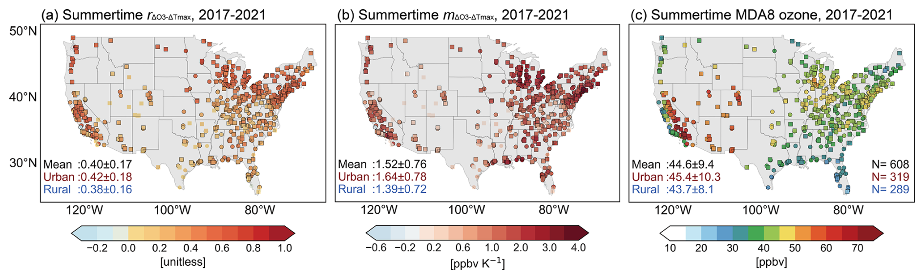
Figure 2 Present-day summertime ozone concentrations and ozone–temperature sensitivity in the continental US. (a, b) Distribution of summertime (June, July, August) $r_{\mathrm{\Delta }{\mathrm{O}}_{\mathrm{3}}-\mathrm{\Delta }{T}_{\text{max}}}$ and $m_{\mathrm{\Delta }{\mathrm{O}}_{\mathrm{3}}-\mathrm{\Delta }{T}_{\text{max}}}$ at individual sites averaged in 2017–2021. The black borders indicate sites with a p value < 0.01 for $r_{\mathrm{\Delta }{\mathrm{O}}_{\mathrm{3}}-\mathrm{\Delta }{T}_{\text{max}}}$ or $m_{\mathrm{\Delta }{\mathrm{O}}_{\mathrm{3}}-\mathrm{\Delta }{T}_{\text{max}}}$. (c) Summer mean MDA8 ozone concentrations at individual sites. Urban sites are represented by circles and rural sites by squares. Mean values and standard deviations over the sites are shown in the inset.

3 Results

3.1 Present-day level of and trends in summertime ozone–temperature sensitivity in the continental US

Figure 2a presents the widespread positive correlation coefficients between summertime daily MDA8 ozone and T_max ($r_{\mathrm{\Delta }{\mathrm{O}}_{\mathrm{3}}-\mathrm{\Delta }{T}_{\text{max}}}$) across the CONUS sites. A total of 604 out of the 608 sites show positive $r_{\mathrm{\Delta }{\mathrm{O}}_{\mathrm{3}}-\mathrm{\Delta }{T}_{\text{max}}}$ (568 sites with a p value < 0.01) in the present day (2017–2021), with a mean $r_{\mathrm{\Delta }{\mathrm{O}}_{\mathrm{3}}-\mathrm{\Delta }{T}_{\text{max}}}$ value of 0.40 ± 0.17 (mean ± standard deviation across the sites) averaged over all sites. Urban sites show slightly higher $r_{\mathrm{\Delta }{\mathrm{O}}_{\mathrm{3}}-\mathrm{\Delta }{T}_{\text{max}}}$ values than rural sites. Figure 2b shows that the present-day mean $m_{\mathrm{\Delta }{\mathrm{O}}_{\mathrm{3}}-\mathrm{\Delta }{T}_{\text{max}}}$ (see Sect. 2.3 for the definition) values averaged for the 608 sites are 1.52 ± 0.76 ppbv K⁻¹, with the $m_{\mathrm{\Delta }{\mathrm{O}}_{\mathrm{3}}-\mathrm{\Delta }{T}_{\text{max}}}$ values at urban sites being higher by 18 % than those averaged for the rural sites (1.64 ± 0.78 versus 1.39 ± 0.72 ppbv K⁻¹). These results reflect the expected ozone increases with temperature in NO_x-rich environments, which are more commonly found in urban areas than in rural areas.

We find distinct variability in the spatial distributions of both $r_{\mathrm{\Delta }{\mathrm{O}}_{\mathrm{3}}-\mathrm{\Delta }{T}_{\text{max}}}$ and $m_{\mathrm{\Delta }{\mathrm{O}}_{\mathrm{3}}-\mathrm{\Delta }{T}_{\text{max}}}$ (Fig. 2, Table S3 in the Supplement). The Midwest and NEUS regions show the highest mean $m_{\mathrm{\Delta }{\mathrm{O}}_{\mathrm{3}}-\mathrm{\Delta }{T}_{\text{max}}}$ values, reaching 2.05 ± 0.62 ($r_{\mathrm{\Delta }{\mathrm{O}}_{\mathrm{3}}-\mathrm{\Delta }{T}_{\text{max}}}$ = 0.50 ± 0.12) and 1.99 ± 0.65 ppbv K⁻¹ ($r_{\mathrm{\Delta }{\mathrm{O}}_{\mathrm{3}}-\mathrm{\Delta }{T}_{\text{max}}}$ = 0.52 ± 0.09), followed by NWUS, with a mean $m_{\mathrm{\Delta }{\mathrm{O}}_{\mathrm{3}}-\mathrm{\Delta }{T}_{\text{max}}}$ of 1.54 ± 0.38 ppbv K⁻¹ ($r_{\mathrm{\Delta }{\mathrm{O}}_{\mathrm{3}}-\mathrm{\Delta }{T}_{\text{max}}}$ = 0.63 ± 0.07). The Intermountain West and Plains regions show the lowest mean $m_{\mathrm{\Delta }{\mathrm{O}}_{\mathrm{3}}-\mathrm{\Delta }{T}_{\text{max}}}$ of less than 1.1 ppbv K⁻¹ in both urban and rural sites with mean $r_{\mathrm{\Delta }{\mathrm{O}}_{\mathrm{3}}-\mathrm{\Delta }{T}_{\text{max}}}$ lower than 0.26, indicating daily ozone variation in this region is not strongly affected by temperature. We also find that the spatial distribution of ozone–temperature sensitivity does not follow that of the MDA8 ozone level (Fig. 2c), as the highest summertime MDA8 ozone concentrations are over the SWUS and Intermountain West regions. The higher $m_{\mathrm{\Delta }{\mathrm{O}}_{\mathrm{3}}-\mathrm{\Delta }{T}_{\text{max}}}$ in the NEUS and Midwest regions than in other regions may reflect the stronger daily variation in ozone due to a rapid shift of synoptic patterns (e.g., mid-latitude cyclones) in this region during summer (Leibensperger et al., 2008). Additionally, changes in other mid-latitude dynamic systems, such as meridional movement by the mid-latitude jet, also play a significant role in shaping the regional ozone–temperature sensitivity (Barnes and Fiore, 2013; Kerr et al., 2020; Zhang et al., 2022c). We observe a decreasing gradient in both $r_{\mathrm{\Delta }{\mathrm{O}}_{\mathrm{3}}-\mathrm{\Delta }{T}_{\text{max}}}$ and $m_{\mathrm{\Delta }{\mathrm{O}}_{\mathrm{3}}-\mathrm{\Delta }{T}_{\text{max}}}$ from north to south in the eastern US, which aligns with previous findings (Camalier et al., 2007; Tawfik and Steiner, 2013). This observed north-to-south shift may be related to the transition in land–atmosphere coupling mechanisms due to soil moisture limitations in the southern regions (Tawfik and Steiner, 2013). The low $m_{\mathrm{\Delta }{\mathrm{O}}_{\mathrm{3}}-\mathrm{\Delta }{T}_{\text{max}}}$ in the Intermountain West region largely reflects the strong background ozone influences (including stratospheric intrusion and long-range transport of wildfire or anthropogenic plumes) instead of local photochemical production (Jaffe et al., 2018; Zhang et al., 2014). These background sources may contribute to high ozone there but are not directly modulated by local temperature.

Previous studies have reported a decrease in ozone concentration at extremely high temperatures over the US (Shen et al., 2016; Steiner et al., 2010). Here we investigate how the suppression of ozone concentration influences the overall ozone–temperature sensitivity. We identify occurrences of ozone suppression and the critical temperature (i.e., beyond which ozone increases are suppressed) at individual sites every year following the criteria described in Ning et al. (2022). We find that while ozone suppression at extremely high temperatures can be detected at 477 out of 608 sites in 2017–2021, excluding data above the critical temperature only changes the present-day mean $m_{\mathrm{\Delta }{\mathrm{O}}_{\mathrm{3}}-\mathrm{\Delta }{T}_{\text{max}}}$ by 2.6 %. This indicates that such a phenomenon does not change the overall positive ozone–temperature sensitivity.

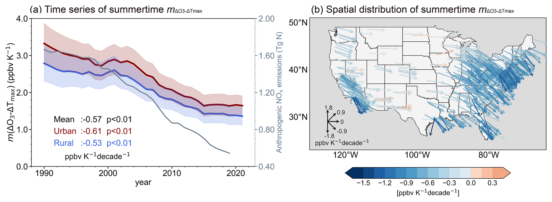
Figure 3 Observed decrease in summertime ozone–temperature sensitivity in 1990–2021. (a) Time series of the summertime $m_{\mathrm{\Delta }{\mathrm{O}}_{\mathrm{3}}-\mathrm{\Delta }{T}_{\text{max}}}$ averaged over the CONUS sites, with a 5-year smoothing average applied to the yearly $m_{\mathrm{\Delta }{\mathrm{O}}_{\mathrm{3}}-\mathrm{\Delta }{T}_{\text{max}}}$ to filter the interannual variability. $m_{\mathrm{\Delta }{\mathrm{O}}_{\mathrm{3}}-\mathrm{\Delta }{T}_{\text{max}}}$ values for urban and rural sites are shown with red and blue lines, respectively. The shaded areas represent the range of mean values ± 30 % standard deviation across the sites. The CONUS $m_{\mathrm{\Delta }{\mathrm{O}}_{\mathrm{3}}-\mathrm{\Delta }{T}_{\text{max}}}$ trends are shown in the inset. Anthropogenic NO_x emissions in the CONUS are shown with the gray line. (b) Spatial distributions of long-term trends in $m_{\mathrm{\Delta }{\mathrm{O}}_{\mathrm{3}}-\mathrm{\Delta }{T}_{\text{max}}}$ in 1990–2021 across the US. Only sites with $r_{\mathrm{\Delta }{\mathrm{O}}_{\mathrm{3}}-\mathrm{\Delta }{T}_{\text{max}}}$ p value < 0.01 are shown. Both directions and colors of the vectors indicate the $m_{\mathrm{\Delta }{\mathrm{O}}_{\mathrm{3}}-\mathrm{\Delta }{T}_{\text{max}}}$ trends.

The present-day (2017–2021) ozone–temperature sensitivity is lower than the reported values for earlier years (i.e., 2–7 ppbv K⁻¹ reported in 2000; Bloomer et al., 2009; Fu et al., 2015; Rasmussen et al., 2013), though different definitions of ozone–temperature sensitivity were applied, suggesting that the ozone–temperature sensitivity may have experienced significant reduction in recent decades. Figure 3 illustrates this feature from long-term observations in 1990–2021. We find in Fig. 3a that mean $m_{\mathrm{\Delta }{\mathrm{O}}_{\mathrm{3}}-\mathrm{\Delta }{T}_{\text{max}}}$ for the CONUS decreased by 50 % from 3.0 ppbv K⁻¹ in 1990 to 1.5 ppbv K⁻¹ in 2021 with a mean decreasing rate of −0.57 ppbv K⁻¹ per decade (p < 0.01). $m_{\mathrm{\Delta }{\mathrm{O}}_{\mathrm{3}}-\mathrm{\Delta }{T}_{\text{max}}}$ over the CONUS urban sites was higher than that over rural sites by 0.50 ppbv K⁻¹ in the early 1990s. However, urban sites exhibit a faster decline rate of $m_{\mathrm{\Delta }{\mathrm{O}}_{\mathrm{3}}-\mathrm{\Delta }{T}_{\text{max}}}$ (−0.61 ppbv K⁻¹ per decade, p < 0.01) compared to rural sites (−0.53 ppbv K⁻¹ per decade, p < 0.01), narrowing the disparity in $m_{\mathrm{\Delta }{\mathrm{O}}_{\mathrm{3}}-\mathrm{\Delta }{T}_{\text{max}}}$ between the two. At the same time, the mean $r_{\mathrm{\Delta }{\mathrm{O}}_{\mathrm{3}}-\mathrm{\Delta }{T}_{\text{max}}}$ decreased from 0.51 in 1990 to 0.40 in 2021 (Fig. S3 in the Supplement). The significant decreases in both $m_{\mathrm{\Delta }{\mathrm{O}}_{\mathrm{3}}-\mathrm{\Delta }{T}_{\text{max}}}$ and $r_{\mathrm{\Delta }{\mathrm{O}}_{\mathrm{3}}-\mathrm{\Delta }{T}_{\text{max}}}$ imply a much weaker response of ozone to temperature in the present day compared to that 3 decades ago. While some studies have shown observed decreases in some regions (e.g., California, as described in Steiner et al., 2010), such significant decreases in ozone–temperature sensitivity over the CONUS have not been presented in previous studies to the best of our knowledge.

The decreasing trends in $m_{\mathrm{\Delta }{\mathrm{O}}_{\mathrm{3}}-\mathrm{\Delta }{T}_{\text{max}}}$ are widespread across the CONUS sites (Fig. 3b), but spatial and temporal variabilities exist. A total of 419 sites (69 %) out of the 608 sites show negative trends with p < 0.01 (492 sites with p < 0.05). The largest decreases are in the NEUS region, where $m_{\mathrm{\Delta }{\mathrm{O}}_{\mathrm{3}}-\mathrm{\Delta }{T}_{\text{max}}}$ values exceeded 4.3 ppbv K⁻¹ in the 1990s but steadily decreased by −0.81 ppbv K⁻¹ per decade, reaching 1.8 ppbv K⁻¹ in 2021. The SWUS region also shows a large decrease in $m_{\mathrm{\Delta }{\mathrm{O}}_{\mathrm{3}}-\mathrm{\Delta }{T}_{\text{max}}}$ by −0.60 ppbv K⁻¹ per decade (p < 0.01). A distinct feature in the SWUS is the notably high urban–rural disparity in $m_{\mathrm{\Delta }{\mathrm{O}}_{\mathrm{3}}-\mathrm{\Delta }{T}_{\text{max}}}$ (4.7 versus 1.9 ppbv K⁻¹) in the early 1990s (Fig. S4 in the Supplement), but this disparity has been significantly reduced as urban sites exhibit a much larger $m_{\mathrm{\Delta }{\mathrm{O}}_{\mathrm{3}}-\mathrm{\Delta }{T}_{\text{max}}}$ trend (−0.88 ppbv K⁻¹ per decade, p < 0.01) than rural sites (−0.34 ppbv K⁻¹ per decade, p < 0.01), particularly in the early 1990s. The SEUS and Midwest regions also show decreases in $m_{\mathrm{\Delta }{\mathrm{O}}_{\mathrm{3}}-\mathrm{\Delta }{T}_{\text{max}}}$, with a mean rate of −0.62 and −0.52 ppbv K⁻¹ per decade. However, we notice an increase in $m_{\mathrm{\Delta }{\mathrm{O}}_{\mathrm{3}}-\mathrm{\Delta }{T}_{\text{max}}}$ in 1990–2000 for the SEUS region and in 1999–2005 for the Plains region (Fig. S4). The increase in ozone–temperature sensitivity in these two regions explains the $m_{\mathrm{\Delta }{\mathrm{O}}_{\mathrm{3}}-\mathrm{\Delta }{T}_{\text{max}}}$ plateau in the CONUS during the 1996–2004 period. Fu et al. (2015) attribute the increased ozone–temperature sensitivity in 1990–2000 in the SEUS to variations in regional ozone advection tied to climate variability. This further underscores the significant influence of climate variability on $m_{\mathrm{\Delta }{\mathrm{O}}_{\mathrm{3}}-\mathrm{\Delta }{T}_{\text{max}}}$ trends. The region with the smallest $m_{\mathrm{\Delta }{\mathrm{O}}_{\mathrm{3}}-\mathrm{\Delta }{T}_{\text{max}}}$ trends is the Intermountain region (−0.08 ppbv K⁻¹ per decade).

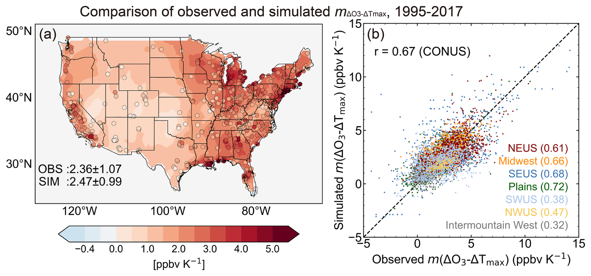
Figure 4 Evaluation of GEOS-Chem-simulated $m_{\mathrm{\Delta }{\mathrm{O}}_{\mathrm{3}}-\mathrm{\Delta }{T}_{\text{max}}}$ in July 1995–2017. (a) Spatial distributions of the observed (circles) and simulated (from the BASE simulation, shaded) $m_{\mathrm{\Delta }{\mathrm{O}}_{\mathrm{3}}-\mathrm{\Delta }{T}_{\text{max}}}$ during July averaged over 1995 to 2017. (b) Scatterplots of the observed and simulated $m_{\mathrm{\Delta }{\mathrm{O}}_{\mathrm{3}}-\mathrm{\Delta }{T}_{\text{max}}}$ for July in each simulated year from 1995 to 2017. Mean values, standard deviations for the CONUS sites from the observation and GEOS-Chem model, and their correlation coefficients (r) in different regions are shown in the inset.

3.2 Simulated long-term trends in ozone–temperature sensitivity and attribution to anthropogenic emission reduction

We now apply the GEOS-Chem chemical transport model to interpret the trends in ozone–temperature sensitivity over the CONUS. Figure S6 in the Supplement compares the spatial distribution of observed and simulated mean surface MDA8 ozone concentrations in July at the 608 sites averaged for 12 years (1995–2017 biennially). Our GEOS-Chem simulation captures the spatial distributions of surface MDA8 ozone across the CONUS, although showing some high bias of MDA8 ozone of 11 ppbv, as also reported in other surface ozone air quality studies using the GEOS-Chem model (Lu et al., 2019a; Travis and Jacob, 2019). Most importantly, the model largely reproduces the spatial pattern of observed $m_{\mathrm{\Delta }{\mathrm{O}}_{\mathrm{3}}-\mathrm{\Delta }{T}_{\text{max}}}$, with a high correlation coefficient of 0.67 and a small positive mean bias of 0.11 ppbv K⁻¹ (4.7 %) at all 608 sites for the monthly $m_{\mathrm{\Delta }{\mathrm{O}}_{\mathrm{3}}-\mathrm{\Delta }{T}_{\text{max}}}$ values (Fig. 4). Table S4 in the Supplement further shows the simulated and observed $m_{\mathrm{\Delta }{\mathrm{O}}_{\mathrm{3}}-\mathrm{\Delta }{T}_{\text{max}}}$ values and their correlation coefficients (r) across different periods and regions. The model demonstrates relatively better performance of $m_{\mathrm{\Delta }{\mathrm{O}}_{\mathrm{3}}-\mathrm{\Delta }{T}_{\text{max}}}$ across the CONUS in 2001–2011 compared to other periods, with a small mean absolute bias (0.01–0.18 ppbv K⁻¹, 1 %–8 %) and high correlation coefficients (0.67–0.70). The simulated $m_{\mathrm{\Delta }{\mathrm{O}}_{\mathrm{3}}-\mathrm{\Delta }{T}_{\text{max}}}$ in the eastern US (NEUS, SEUS, Midwest, and Plains) is in better agreement with the observed values than in the western US, with r ranging from 0.50 to 0.76. The above analyses support the suggestion that the GEOS-Chem model captures the overall ozone–temperature sensitivity well in the period of 1995–2017.

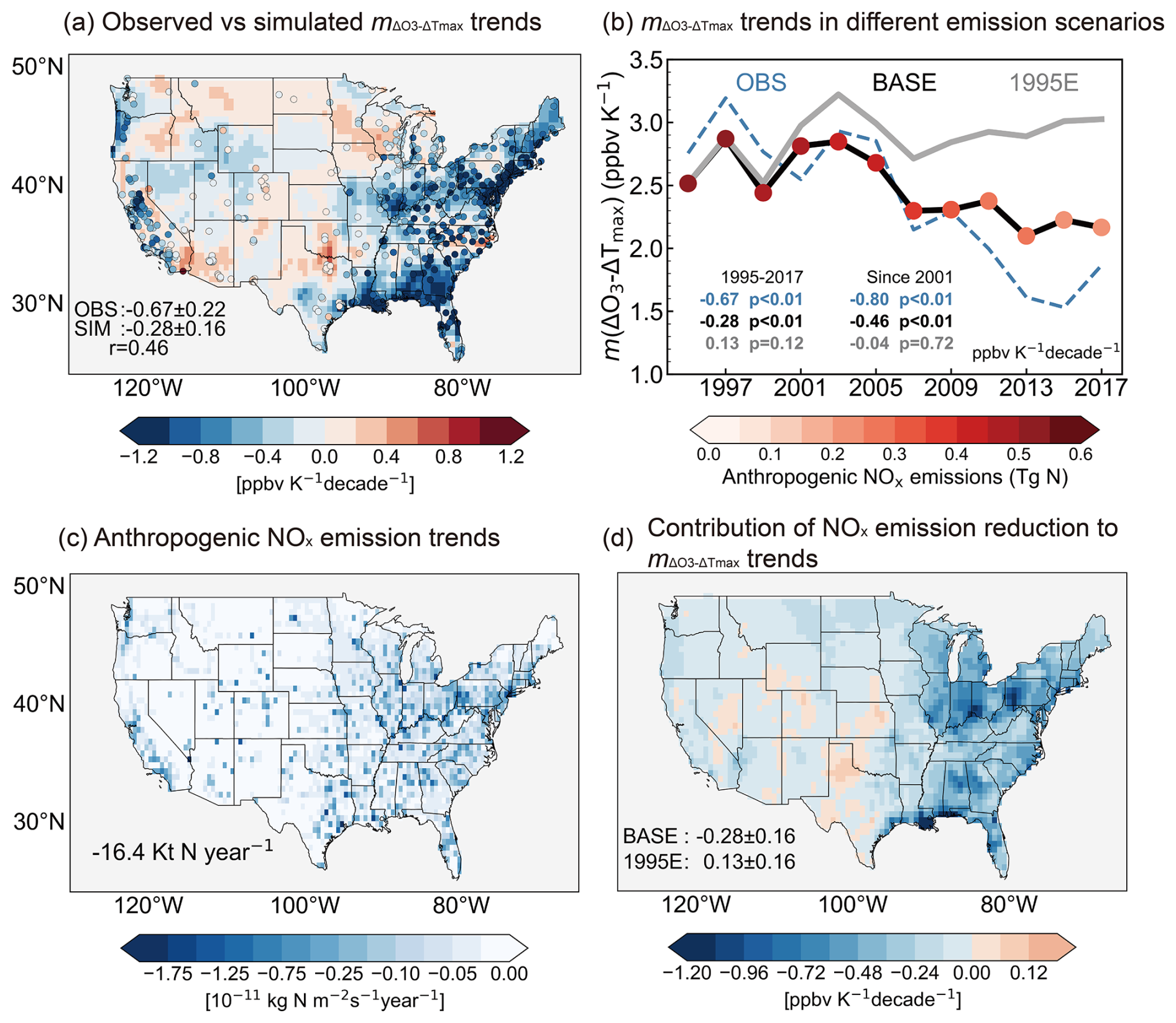
Figure 5 GEOS-Chem-simulated decrease in summertime ozone–temperature sensitivity and the attribution to a reduction in anthropogenic NO_x emission. (a) Spatial distributions of the observed (circles) and simulated (from the BASE simulation, shaded) $m_{\mathrm{\Delta }{\mathrm{O}}_{\mathrm{3}}-\mathrm{\Delta }{T}_{\text{max}}}$ trends during July from 1995 to 2017. Mean trends± 95 % confidence level for the CONUS sites from the observation and GEOS-Chem model, with the correlation coefficients (r) of $m_{\mathrm{\Delta }{\mathrm{O}}_{\mathrm{3}}-\mathrm{\Delta }{T}_{\text{max}}}$ trends between the two shown in the inset. (b) Time series of the observed and simulated $m_{\mathrm{\Delta }{\mathrm{O}}_{\mathrm{3}}-\mathrm{\Delta }{T}_{\text{max}}}$ in July during 1995–2017 (biennially) at CONUS sites. Results from the BASE simulation and a sensitivity simulation with anthropogenic NO_x emissions fixed at the 1995 level (1995E) are compared. The colored circles denote the July anthropogenic NO_x emissions in the CONUS. (c) Spatial distribution of anthropogenic NO_x emission trends during July from 1995 to 2017. Trends are calculated for each model grid. Emissions trends aggregated over the CONUS are insets. (d) Contribution of anthropogenic NO_x emissions to $m_{\mathrm{\Delta }{\mathrm{O}}_{\mathrm{3}}-\mathrm{\Delta }{T}_{\text{max}}}$ trends, estimated as the difference in the $m_{\mathrm{\Delta }{\mathrm{O}}_{\mathrm{3}}-\mathrm{\Delta }{T}_{\text{max}}}$ trend between the BASE and 1995E simulations. Mean trends± 95 % confidence level are shown in the inset.

Figure 5a further compares the observed and GEOS-Chem-simulated 1995–2017 trends in $m_{\mathrm{\Delta }{\mathrm{O}}_{\mathrm{3}}-\mathrm{\Delta }{T}_{\text{max}}}$ in July across the CONUS. The following analysis applies biennial data from 1995 to 2017 to align with the GEOS-Chem simulations. The overall observed $m_{\mathrm{\Delta }{\mathrm{O}}_{\mathrm{3}}-\mathrm{\Delta }{T}_{\text{max}}}$ trends in July, as depicted in Fig. 5a, are similar to those in the June–July–August period, as presented in Fig. 3b, but there are slight differences at individual sites, reflecting the difference in the time frame. We find that, driven by yearly-varied meteorological fields and anthropogenic emissions, the GEOS-Chem model successfully reproduces the decline in $m_{\mathrm{\Delta }{\mathrm{O}}_{\mathrm{3}}-\mathrm{\Delta }{T}_{\text{max}}}$ across the CONUS, showing a spatial correlation coefficient of 0.46 with observed $m_{\mathrm{\Delta }{\mathrm{O}}_{\mathrm{3}}-\mathrm{\Delta }{T}_{\text{max}}}$ trends (p < 0.01). In particular, the model reproduces the much larger $m_{\mathrm{\Delta }{\mathrm{O}}_{\mathrm{3}}-\mathrm{\Delta }{T}_{\text{max}}}$ decreases in the eastern CONUS (the NEUS, Midwest, and SEUS) compared to other regions, consistent with the observations. However, the model has difficulty in capturing the magnitude of observed $m_{\mathrm{\Delta }{\mathrm{O}}_{\mathrm{3}}-\mathrm{\Delta }{T}_{\text{max}}}$ trends. The model shows a mean $m_{\mathrm{\Delta }{\mathrm{O}}_{\mathrm{3}}-\mathrm{\Delta }{T}_{\text{max}}}$ trend of −0.28 ppbv K⁻¹ per decade over the CONUS that accounts for 42 % of the observed trends of −0.67 ppbv K⁻¹ per decade. Figure 5b also shows that the model's underestimation of $m_{\mathrm{\Delta }{\mathrm{O}}_{\mathrm{3}}-\mathrm{\Delta }{T}_{\text{max}}}$ trends is primarily attributed to an overestimation of $m_{\mathrm{\Delta }{\mathrm{O}}_{\mathrm{3}}-\mathrm{\Delta }{T}_{\text{max}}}$ from 2013 to 2017 and an underestimation from 1995 to 1999. The consistency between the observed and simulated $m_{\mathrm{\Delta }{\mathrm{O}}_{\mathrm{3}}-\mathrm{\Delta }{T}_{\text{max}}}$ trends also shows regional differences. As shown in Fig. S8 in the Supplement, the model reproduces the interannual variation in $m_{\mathrm{\Delta }{\mathrm{O}}_{\mathrm{3}}-\mathrm{\Delta }{T}_{\text{max}}}$ well in the Plains and Intermountain West regions and also captures 65 % of the observed trend in the NWUS. However, in other regions, the model captures only less than 50 % of the observed $m_{\mathrm{\Delta }{\mathrm{O}}_{\mathrm{3}}-\mathrm{\Delta }{T}_{\text{max}}}$ trends, with either an overestimation in 2013–2017 or an underestimation in 1995–1999.

Our GEOS-Chem simulation has successfully reproduced the observed long-term ozone trend averaged over the CONUS (−6.1 ppbv per decade in GEOS-Chem vs. −6.5 ppbv per decade in observations) (Table S5 in the Supplement). However, capturing the long-term trends in $m_{\mathrm{\Delta }{\mathrm{O}}_{\mathrm{3}}-\mathrm{\Delta }{T}_{\text{max}}}$ can be more challenging than capturing those in ozone concentrations, as it involves the combined uncertainty in temperature data, simulated ozone concentrations, and the parameterization of the ozone–temperature response. The underestimation of $m_{\mathrm{\Delta }{\mathrm{O}}_{\mathrm{3}}-\mathrm{\Delta }{T}_{\text{max}}}$ from 1995 to 1999 may partly be attributed to the larger bias in the MERRA-2 temperature dataset compared to other periods (Fig. S1), and such bias can propagate to the derivation of observed $m_{\mathrm{\Delta }{\mathrm{O}}_{\mathrm{3}}-\mathrm{\Delta }{T}_{\text{max}}}$ based on the MERRA-2 dataset. Excluding the 1995, 1997, and 1999 records improves the model's ability to capture observed $m_{\mathrm{\Delta }{\mathrm{O}}_{\mathrm{3}}-\mathrm{\Delta }{T}_{\text{max}}}$ trends in the CONUS (−0.46 ppbv K⁻¹ per decade in GEOS-Chem vs. −0.80 ppbv K⁻¹ per decade, 58 %). In particular, for the NEUS, Midwest, and SWUS, the model's ability to capture observed $m_{\mathrm{\Delta }{\mathrm{O}}_{\mathrm{3}}-\mathrm{\Delta }{T}_{\text{max}}}$ trends improves from 44 %, 49 %, and 23 % to 83 %, 66 %, and 54 %, respectively. The simulated ozone–temperature sensitivity for 2013–2017 shows an overestimation, particularly in the SEUS and Midwest regions (Fig. S8). Christiansen et al. (2024) suggested that the CEDS inventory overestimates post-2010 anthropogenic NO_x emissions, especially in the eastern US, which may lead to overestimation of ozone–temperature sensitivity in these regions. The GEOS-Chem model also misses several pathways in describing the responses of ozone to temperature, such as the response of anthropogenic emissions to the external environment and land–atmosphere interaction through soil and vegetation. This is discussed in detail in Sect. 4. We do not further differentiate the simulated $m_{\mathrm{\Delta }{\mathrm{O}}_{\mathrm{3}}-\mathrm{\Delta }{T}_{\text{max}}}$ trends at urban and rural sites because the model resolution at about 50 km may be too coarse for such separation.

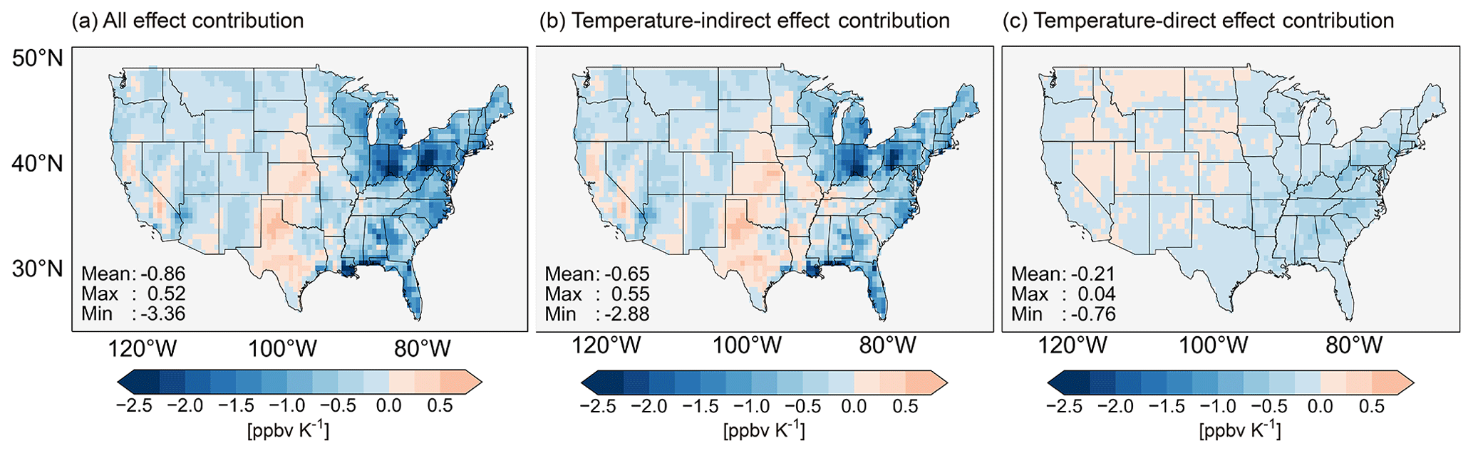
Figure 6 Mechanisms for the decrease in $m_{\mathrm{\Delta }{\mathrm{O}}_{\mathrm{3}}-\mathrm{\Delta }{T}_{\text{max}}}$ with anthropogenic NO_x emission reduction. (a) Changes in $m_{\mathrm{\Delta }{\mathrm{O}}_{\mathrm{3}}-\mathrm{\Delta }{T}_{\text{max}}}$ due to the difference in anthropogenic NO_x emissions in 2017 and 1995, estimated as the difference in $m_{\mathrm{\Delta }{\mathrm{O}}_{\mathrm{3}}-\mathrm{\Delta }{T}_{\text{max}}}$ between the BASE and 1995E simulation for July 2017. (b) The contribution of the temperature indirect effect to $m_{\mathrm{\Delta }{\mathrm{O}}_{\mathrm{3}}-\mathrm{\Delta }{T}_{\text{max}}}$ with changes in anthropogenic NO_x emissions, estimated as the difference in $m_{\mathrm{\Delta }{\mathrm{O}}_{\mathrm{3}}-\mathrm{\Delta }{T}_{\text{max}}}$ between BASE-FTEMP and 1995E-FTEMP (Sect. 2.4). (c) The contribution of the temperature direct effect, estimated as the difference in $m_{\mathrm{\Delta }{\mathrm{O}}_{\mathrm{3}}-\mathrm{\Delta }{T}_{\text{max}}}$ between BASE and 1995E minus the difference between BASE-FTEMP and 1995E-FTEMP. Mean, maximum, and minimum values of the contributions among all CONUS sites are shown in the inset.

Previous studies have implied reductions in anthropogenic emissions would result in a decrease in the ozone–temperature sensitivity (Bloomer et al., 2009). Here we explicitly test this theory using our sensitivity experiments with anthropogenic NO_x emissions in US fixed at the 1995 level (1995E). Figure 5b shows that once the anthropogenic NO_x emissions were fixed in 1995, the GEOS-Chem model simulated no decrease in $m_{\mathrm{\Delta }{\mathrm{O}}_{\mathrm{3}}-\mathrm{\Delta }{T}_{\text{max}}}$ (instead, it simulated a positive trend by 0.13 ppbv K⁻¹ per decade averaged over all sites, p = 0.12). This implies that the change in anthropogenic NO_x emissions alone decreases $m_{\mathrm{\Delta }{\mathrm{O}}_{\mathrm{3}}-\mathrm{\Delta }{T}_{\text{max}}}$ by −0.41 ppbv K⁻¹ per decade for all 608 sites, compared to the observed $m_{\mathrm{\Delta }{\mathrm{O}}_{\mathrm{3}}-\mathrm{\Delta }{T}_{\text{max}}}$ trend of −0.67 ppbv K⁻¹ per decade, and is apparently the dominant driver of the observed decrease in $m_{\mathrm{\Delta }{\mathrm{O}}_{\mathrm{3}}-\mathrm{\Delta }{T}_{\text{max}}}$. In comparison, the simulation with only anthropogenic VOC emissions fixed at the 1995 level shows a negligible difference in $m_{\mathrm{\Delta }{\mathrm{O}}_{\mathrm{3}}-\mathrm{\Delta }{T}_{\text{max}}}$ compared to the BASE simulation. We note that the difference in the $m_{\mathrm{\Delta }{\mathrm{O}}_{\mathrm{3}}-\mathrm{\Delta }{T}_{\text{max}}}$ trend between the BASE and 1995E simulations is highly consistent with the spatial distribution of anthropogenic NO_x emission trends (r = 0.40, p < 0.01) (Fig. 5c), further confirming that NO_x emission reduction is an important driver of the decline in $m_{\mathrm{\Delta }{\mathrm{O}}_{\mathrm{3}}-\mathrm{\Delta }{T}_{\text{max}}}$. Figure S8 illustrates that the regions with $m_{\mathrm{\Delta }{\mathrm{O}}_{\mathrm{3}}-\mathrm{\Delta }{T}_{\text{max}}}$ being mostly affected by anthropogenic NO_x emission reductions are located in the eastern CONUS (the NEUS, Midwest, and SEUS), while other regions are less affected.

3.3 The underlying mechanisms for the decrease in ozone–temperature sensitivity with reduced NO_x emissions

Our analyses above prove that the reduction in anthropogenic NO_x emissions is the dominant driver of the observed long-term decrease in $m_{\mathrm{\Delta }{\mathrm{O}}_{\mathrm{3}}-\mathrm{\Delta }{T}_{\text{max}}}$ in the CONUS. We next examine how the changes in anthropogenic NO_x emissions have altered processes controlling ozone's response to temperature. Previous studies have shown that temperature's impacts on surface ozone concentrations involve acceleration of chemical reaction rates (in particular the thermal decomposition of PAN), increased natural emissions of BVOCs and soil reactive nitrogen, and inhabitation of ozone dry deposition (Lu et al., 2019b; Porter and Heald, 2019; Steiner et al., 2010). Some studies have also argued that the temperature-related covariance with other meteorological phenomena, such as drought (low humidity), stagnancy, and transport, may be more important in determining $m_{\mathrm{\Delta }{\mathrm{O}}_{\mathrm{3}}-\mathrm{\Delta }{T}_{\text{max}}}$ (Kerr et al., 2019; Porter and Heald, 2019; Zhang et al., 2022a, c). Based on these previous studies, we focus on the changes in these impacts on $m_{\mathrm{\Delta }{\mathrm{O}}_{\mathrm{3}}-\mathrm{\Delta }{T}_{\text{max}}}$ with anthropogenic emission reduction in the US.

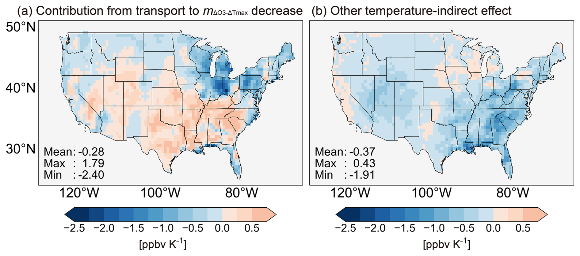
Figure 7 The different temperature indirect effects for the decrease in $m_{\mathrm{\Delta }{\mathrm{O}}_{\mathrm{3}}-\mathrm{\Delta }{T}_{\text{max}}}$ with anthropogenic NO_x emission reduction. (a) The contribution of the transport to $m_{\mathrm{\Delta }{\mathrm{O}}_{\mathrm{3}}-\mathrm{\Delta }{T}_{\text{max}}}$ decrease with changes in anthropogenic NO_x emissions, estimated as the difference in $m_{\mathrm{\Delta }{\mathrm{O}}_{\mathrm{3}}-\mathrm{\Delta }{T}_{\text{max}}}$ between BASE-TRANS and 1995E-TRANS (Sect. 2.4). (b) The contribution of the other temperature indirect effect, estimated as the difference in $m_{\mathrm{\Delta }{\mathrm{O}}_{\mathrm{3}}-\mathrm{\Delta }{T}_{\text{max}}}$ between BASE-FTEMP and 1995E-FTEMP minus the difference between BASE-TRANS and 1995E-TRANS. Mean, maximum, and minimum values of the contributions among all CONUS sites are shown in the inset.

We illustrate in Fig. 6 the simulated changes in $m_{\mathrm{\Delta }{\mathrm{O}}_{\mathrm{3}}-\mathrm{\Delta }{T}_{\text{max}}}$ in July 2017 through temperature direct effects and temperature indirect effects associated with the anthropogenic reduction in NO_x. Figure 6a shows that the reduction in anthropogenic NO_x emissions from 1995 to 2017 alone decreased $m_{\mathrm{\Delta }{\mathrm{O}}_{\mathrm{3}}-\mathrm{\Delta }{T}_{\text{max}}}$ by 0.86 ppbv K⁻¹ in July 2017 (estimated as the difference between the BASE simulation and 1995E simulation). The decreases are larger in the eastern US (including the NEUS, Midwest, and SEUS), reaching 1.37, 1.28, and 1.00 ppbv K⁻¹, respectively. When the temperature direct effect was completely removed from the GEOS-Chem simulation (Sect. 2.4), the reduction in anthropogenic NO_x emissions from 1995 to 2017 decreased $m_{\mathrm{\Delta }{\mathrm{O}}_{\mathrm{3}}-\mathrm{\Delta }{T}_{\text{max}}}$ by 0.65 ppbv K⁻¹ in July 2017. This indicates that only a relatively small portion of the decrease in $m_{\mathrm{\Delta }{\mathrm{O}}_{\mathrm{3}}-\mathrm{\Delta }{T}_{\text{max}}}$ (24 %, 0.21 ppbv K⁻¹ compared with 0.86 ppbv K⁻¹) with anthropogenic NO_x reduction can be attributed to the temperature direct effect (Fig. 6c), while the remainder is explained by the temperature indirect effect. Our results agree with Porter and Heald (2019), which shows that the collinearity between temperature and other meteorological variables played a significant role in determining the overall ozone–temperature relationship. Here, we further demonstrate that the temperature indirect effect also dominates the decline in ozone–temperature sensitivity with anthropogenic NO_x emission reduction.

The temperature indirect effect on ozone mainly includes the influence of temperature-relevant meteorological parameters, such as humidity (as an indicator of the content of water vapor) and shortwave radiation, on ozone photochemistry and also the effect of transport (including stagnancy and regional transport). We further distinguish the impact of transport (by normalizing all meteorological elements except the three-dimensional wind field and PBLH as input in the GEOS-Chem model) and the other indirect effects on the decrease in $m_{\mathrm{\Delta }{\mathrm{O}}_{\mathrm{3}}-\mathrm{\Delta }{T}_{\text{max}}}$ with emission reduction. As shown in Fig. 7, transport (−0.28 ppbv K⁻¹) and other indirect effects (−0.37 ppbv K⁻¹) such as humidity and radiation show a comparable contribution to the decline in $m_{\mathrm{\Delta }{\mathrm{O}}_{\mathrm{3}}-\mathrm{\Delta }{T}_{\text{max}}}$, but the spatial patterns show large disparity. The temperature indirect effect excluding transport (Fig. 7b) on $m_{\mathrm{\Delta }{\mathrm{O}}_{\mathrm{3}}-\mathrm{\Delta }{T}_{\text{max}}}$ shows a more uniform decline with reduced emissions in most regions across the CONUS, with a larger decrease in the southeastern US. The radiation received by vegetation in the southeastern US is highly collinear with temperature and also plays an important role in BVOC emissions (Guenther et al., 2012), which may reflect that its potential for ozone formation reduces with the decline in anthropogenic NO_x emissions. In comparison, the transport effect has larger impacts on the $m_{\mathrm{\Delta }{\mathrm{O}}_{\mathrm{3}}-\mathrm{\Delta }{T}_{\text{max}}}$ trend (Fig. 7a) with reduced NO_x emissions in the northeastern US, where transport has the largest contribution to the mean $m_{\mathrm{\Delta }{\mathrm{O}}_{\mathrm{3}}-\mathrm{\Delta }{T}_{\text{max}}}$ values (Fig. S10), as also reported in Kerr et al. (2019). Some studies have demonstrated that changes in mid-latitude weather systems can significantly influence ozone–temperature sensitivity by affecting pollutant transport (Barnes and Fiore, 2013; Kerr et al., 2020), which could be the underlying mechanism explaining the role of transport in contributing to the decrease in ozone–temperature sensitivity with emission reductions. However, we find that these effects cause an increase in $m_{\mathrm{\Delta }{\mathrm{O}}_{\mathrm{3}}-\mathrm{\Delta }{T}_{\text{max}}}$ in the southern US in July 2017. Nevertheless, the impact of transport on $m_{\mathrm{\Delta }{\mathrm{O}}_{\mathrm{3}}-\mathrm{\Delta }{T}_{\text{max}}}$ largely depends on the transport pattern itself, and it should ideally be investigated through long-term simulations rather than the 1-month study we conducted.

Figure 8 The different temperature direct effects for the decrease in $m_{\mathrm{\Delta }{\mathrm{O}}_{\mathrm{3}}-\mathrm{\Delta }{T}_{\text{max}}}$ with anthropogenic NO_x emission reduction. (a) Combined contribution of the four temperature-dependent mechanisms (BVOC emissions, dry deposition, PAN decomposition, and soil NO_x emissions) to $m_{\mathrm{\Delta }{\mathrm{O}}_{\mathrm{3}}-\mathrm{\Delta }{T}_{\text{max}}}$ with changes in anthropogenic NO_x emissions, estimated as the difference in $m_{\mathrm{\Delta }{\mathrm{O}}_{\mathrm{3}}-\mathrm{\Delta }{T}_{\text{max}}}$ between BASE and 1995E minus the difference between BASE-F4PATHS and 1995E-F4PATHS (Sect. 2.4). (b–e) Individual contribution of BVOC emissions, dry deposition, PAN decomposition, and soil NO_x emissions to $m_{\mathrm{\Delta }{\mathrm{O}}_{\mathrm{3}}-\mathrm{\Delta }{T}_{\text{max}}}$ with changes in anthropogenic NO_x emissions, respectively. Mean, maximum, and minimum values of the contributions among all CONUS sites are shown in the inset. Note that the data range of each figure is different.

The temperature direct effects on ozone–temperature sensitivity include the explicit impacts of temperature on BVOC and soil NO_x emissions, chemical kinetics, and dry deposition. Figure 8 shows the additive and individual impacts from the four temperature-dependent mechanisms (BVOCs, dry deposition, PAN decomposition, and soil NO_x) on the decrease in $m_{\mathrm{\Delta }{\mathrm{O}}_{\mathrm{3}}-\mathrm{\Delta }{T}_{\text{max}}}$ with reduced NO_x emissions. Comparison of Fig. 8a with Fig. 6c shows that the four temperature-dependent mechanisms contribute to almost all of the $m_{\mathrm{\Delta }{\mathrm{O}}_{\mathrm{3}}-\mathrm{\Delta }{T}_{\text{max}}}$ decreases, attributable to the temperature direct effect (−0.19 ppbv K⁻¹ versus −0.21 ppbv K⁻¹).

We find that the ozone–temperature sensitivity contributed by BVOC emissions has reduced significantly with anthropogenic emission control (Fig. 8b). In July 2017, BVOC emissions alone would have contributed to ozone–temperature sensitivity by 0.2 ppbv K⁻¹ if anthropogenic emissions had remained at 1995 levels, with a particularly large contribution of 0.5 ppbv K⁻¹ over the parts of the eastern US where anthropogenic NO_x emissions are high and ozone formation is sensitive to VOC emissions (Fig. S11d in the Supplement). However, with anthropogenic NO_x emission decreased to the 2017 level, the contribution of BVOC emissions decreases to 0.03 ppbv K⁻¹ averaged over the CONUS sites and −0.01 ppbv K⁻¹ averaged over the SEUS region (Fig. S11c). This suggests that the reduction in anthropogenic NO_x emission has shifted the ozone formation regime to a less VOC-sensitive state, in which ozone concentrations are much less sensitive to increased BVOCs at high temperatures. Ozone–temperature sensitivity contributed by dry deposition also reduced by −0.03 ppbv K⁻¹ averaged over the CONUS sites with anthropogenic emission reduction (Fig. 8c).

Figure 9 Decreased $m_{\mathrm{\Delta }{\mathrm{O}}_{\mathrm{3}}-\mathrm{\Delta }{T}_{\text{max}}}$ offers an ozone mitigation benefit at high temperatures. (a) Simulated ozone concentration in different T_max bins in the state of New York in July 2013, 2015, and 2017. Data are binned to 2 K intervals. Results from the BASE simulation (black) and 1995E simulation (gray) are shown. The blue bars represent the ozone enhancement for each temperature bin compared to 291 K from the BASE simulation. The bar marked by the gray border denotes ozone enhancement for each temperature bin compared to 291 K from the 1995E simulation. Thus, the red bar (difference between the gray and blue bars) shows the estimation of the decrease in ozone enhancement due to the reduction in anthropogenic emissions from 1995 to 2017. (b) Distributions of the ozone mitigation benefit in July due to the decreased $m_{\mathrm{\Delta }{\mathrm{O}}_{\mathrm{3}}-\mathrm{\Delta }{T}_{\text{max}}}$, estimated as the ozone enhancement from the lowest 0 %–10 % to the highest 90 %–100 % temperature bins in the 1995E simulation minus those in the BASE simulation at each grid in July (2013, 2015, and 2017). Mean, max, and min values for the 608 sites are shown in the inset.

The thermal decomposition of PAN contributes to 0.43 ppbv K⁻¹ of the overall $m_{\mathrm{\Delta }{\mathrm{O}}_{\mathrm{3}}-\mathrm{\Delta }{T}_{\text{max}}}$ over the CONUS (Fig. S11g), with a larger contribution of 0.7 ppbv K⁻¹ over the eastern US. This is also consistent with Porter and Heald (2019), which shows the PAN decomposition explains a large fraction of the ozone–temperature sensitivity compared to other mechanisms such as BVOC emissions and dry deposition. The PAN concentrations averaged over the CONUS decrease by 27 % with the reduction in anthropogenic NO_x emissions (Fig. S12 in the Supplement). Nevertheless, $m_{\mathrm{\Delta }{\mathrm{O}}_{\mathrm{3}}-\mathrm{\Delta }{T}_{\text{max}}}$ contributed by PAN decomposition only shows a minor change of −0.02 ppbv K⁻¹ with the reduction in anthropogenic NO_x emission averaged over the CONUS (Fig. 8d), reflecting the offset between $m_{\mathrm{\Delta }{\mathrm{O}}_{\mathrm{3}}-\mathrm{\Delta }{T}_{\text{max}}}$ increase in the central and western US and $m_{\mathrm{\Delta }{\mathrm{O}}_{\mathrm{3}}-\mathrm{\Delta }{T}_{\text{max}}}$ decrease in the eastern US. A possible reason is that, with the reduction in anthropogenic NO_x emissions, ozone formation in the central and western US becomes more NO_x sensitive such that the decomposition of PAN increases ozone–temperature sensitivity. The decrease in $m_{\mathrm{\Delta }{\mathrm{O}}_{\mathrm{3}}-\mathrm{\Delta }{T}_{\text{max}}}$ contributed by PAN decomposition in the eastern US may mainly reflect the reduction in PAN concentration with anthropogenic NO_x emission reduction (Fig. S12).

Unlike the other mechanisms, $m_{\mathrm{\Delta }{\mathrm{O}}_{\mathrm{3}}-\mathrm{\Delta }{T}_{\text{max}}}$ contributed by the temperature-dependent soil NO_x emissions increases by 0.03 ppbv K⁻¹ averaged over the CONUS with anthropogenic NO_x emission reduction. The increase in $m_{\mathrm{\Delta }{\mathrm{O}}_{\mathrm{3}}-\mathrm{\Delta }{T}_{\text{max}}}$ reflects the competitive effect between natural soil (from both natural pools and agricultural fertilizer, conventionally categorized as natural sources) and anthropogenic (from fossil fuel) NO_x emissions on ozone formation (Lu et al., 2021; Tan et al., 2023). Soil emissions become an increasingly important source of nitrogen for ozone formation with decreased anthropogenic NO_x emission levels (Guo et al., 2018; Geddes et al., 2022). As soil emissions are larger at higher temperatures, they contribute to an increasing ozone–temperature sensitivity. The above analysis reveals the increasing importance of soil NO_x emissions for determining ozone–temperature sensitivity in a future with low anthropogenic NO_x emissions.

3.4 Ozone mitigation benefit through the declined ozone–temperature sensitivity

The significant decrease in $m_{\mathrm{\Delta }{\mathrm{O}}_{\mathrm{3}}-\mathrm{\Delta }{T}_{\text{max}}}$ over the CONUS indicates that controlling anthropogenic emissions reduces not only the mean ozone levels, but also the response of ozone to temperature. Consequently, this reduction lowers the risk of extreme ozone pollution and associated health damage at high temperatures, presenting an appealing benefit of ozone mitigation. We illustrate this benefit by reducing $m_{\mathrm{\Delta }{\mathrm{O}}_{\mathrm{3}}-\mathrm{\Delta }{T}_{\text{max}}}$ in ozone mitigation, taking the state of New York as an example, as it has high $m_{\mathrm{\Delta }{\mathrm{O}}_{\mathrm{3}}-\mathrm{\Delta }{T}_{\text{max}}}$ and a large population that is exposed to ozone pollution. Figure 9a shows the GEOS-Chem-simulated ozone in July for 3 years (2013, 2015, 2017) at different T_max bins. As expected, MDA8 ozone increases with increased temperature. The ozone difference between the highest-temperature bin (307 K) and the lowest-temperature bin (291 K) is 31 ppbv in the BASE simulation, comparable to observations (26 ppbv between 307 and 291 K). If anthropogenic NO_x emissions were fixed at the 1995 level, however, the predicted ozone difference between the 307 and 291 K temperature bins would be enlarged to 41 ppbv. This means that NO_x emission reductions cause an “additional” ozone concentration reduction of 10 ppbv from 291 to 307 K, as reflected in the significant decline in $m_{\mathrm{\Delta }{\mathrm{O}}_{\mathrm{3}}-\mathrm{\Delta }{T}_{\text{max}}}$. Such a benefit of reducing $m_{\mathrm{\Delta }{\mathrm{O}}_{\mathrm{3}}-\mathrm{\Delta }{T}_{\text{max}}}$ is typically larger at higher temperatures. A similar phenomenon can be found in other regions with a significant decrease in $m_{\mathrm{\Delta }{\mathrm{O}}_{\mathrm{3}}-\mathrm{\Delta }{T}_{\text{max}}}$ (Fig. S13 in the Supplement).

Figure 9b further quantifies the beneficial effect of anthropogenic emission reduction on ozone mitigation through reducing $m_{\mathrm{\Delta }{\mathrm{O}}_{\mathrm{3}}-\mathrm{\Delta }{T}_{\text{max}}}$ over the CONUS. This can be estimated as the suppression of ozone increase between high (90–100th percentile of T_max in July 2013, 2015, and 2017) and low temperature ranges (the lowest 10th percentile of T_max) due to anthropogenic NO_x emission reduction from 1995 to 2017. We find that the additional ozone mitigation benefit by reducing $m_{\mathrm{\Delta }{\mathrm{O}}_{\mathrm{3}}-\mathrm{\Delta }{T}_{\text{max}}}$ is 6.8 ppbv averaged across the CONUS. The benefit is more pronounced in the eastern US, where emission reductions are more prominent, reaching a maximum of 19.4 ppbv. This benefit significantly reduces the probability of ozone exceedance (MDA8 ozone >70 ppbv) during high-temperature conditions (above the 90th percentile of T_max), from 70 % (estimated from the 1995E simulation) to 28 % (from the BASE simulation). The results show that emissions controlled on ozone precursors in the US effectively reduced the ozone surge at high temperatures across the CONUS and alleviated the combined health damage of the joint occurrence of heat and ozone extremes, highlighting the importance of continuous anthropogenic emission control for ozone mitigation in a warming future.

4 Summary and discussion

We have estimated in this study the present-day (2017–2021) distributions of and long-term (1990–2021) trends in summertime surface ozone–temperature sensitivity in the CONUS, combining observational monitoring network and GEOS-Chem simulations at a resolution of about 50 km. We find a clear pattern that the observed $m_{\mathrm{\Delta }{\mathrm{O}}_{\mathrm{3}}-\mathrm{\Delta }{T}_{\text{max}}}$ for the CONUS decreased by 50 % from 3.0 ppbv K⁻¹ in 1990 to 1.5 ppbv K⁻¹ in 2021 with a mean decreasing rate of −0.57 ppbv K⁻¹ per decade (p < 0.01), with urban sites showing faster trends than rural sites (−0.61 vs. −0.53 ppbv K⁻¹ per decade), indicating a much weaker response of ozone to temperature in the present day compared to that 3 decades ago. During the period from 1990 to 2021, anthropogenic NO_x emissions in the US decreased by approximately 69 %, and the eastern US, where stricter anthropogenic emission controls were implemented, is the core region where ozone–temperature sensitivity has declined the most. The GEOS-Chem simulations, driven by a year-specific anthropogenic emission inventory and MERRA-2 reanalysis meteorological fields, reproduce the distribution and magnitude of the multi-year mean $m_{\mathrm{\Delta }{\mathrm{O}}_{\mathrm{3}}-\mathrm{\Delta }{T}_{\text{max}}}$ well and capture 42 % of the observed trends in $m_{\mathrm{\Delta }{\mathrm{O}}_{\mathrm{3}}-\mathrm{\Delta }{T}_{\text{max}}}$ in 1995–2017. The model simulation shows that the decline in anthropogenic NO_x emission over the CONUS is the dominant driver of the $m_{\mathrm{\Delta }{\mathrm{O}}_{\mathrm{3}}-\mathrm{\Delta }{T}_{\text{max}}}$ decrease. Mechanically, approximately 76 % of the simulated decline in $m_{\mathrm{\Delta }{\mathrm{O}}_{\mathrm{3}}-\mathrm{\Delta }{T}_{\text{max}}}$ can be attributed to the temperature indirect effects arising from the shared collinearity of other meteorological effects (such as humidity, ventilation, and transport) on ozone. The remaining portion explaining the decrease in $m_{\mathrm{\Delta }{\mathrm{O}}_{\mathrm{3}}-\mathrm{\Delta }{T}_{\text{max}}}$ with anthropogenic NO_x emission reduction is mostly attributed to four direct temperature-dependent processes, in which $m_{\mathrm{\Delta }{\mathrm{O}}_{\mathrm{3}}-\mathrm{\Delta }{T}_{\text{max}}}$ decreases through the pathways of BVOC emissions, dry deposition, and PAN decomposition (mostly in the eastern US), while soil NO_x emissions increase $m_{\mathrm{\Delta }{\mathrm{O}}_{\mathrm{3}}-\mathrm{\Delta }{T}_{\text{max}}}$ with anthropogenic NO_x emission reduction.

Our study illustrates that anthropogenic controls on NO_x emissions significantly reduced the response of surface ozone concentration to variation in temperature, offering a compelling advantage for ozone mitigation at high temperatures. The model simulation estimates that the reduction in anthropogenic NO_x emissions from 1995 to 2017 decreases the ozone enhancement from low to high temperatures by 6.8 ppbv on average across the CONUS (reaching 19 ppbv in parts of the eastern US). Ozone–temperature sensitivity remains a crucial factor in quantifying the impact of climate on ozone. Our research demonstrates that anthropogenic emission changes not only alleviate current ozone pollution but also help mitigate potential future increases in ozone concentrations due to climate change. It also indicates the dependency of ozone–temperature sensitivity on anthropogenic emission levels, which should be considered in projections of future ozone concentrations in a warmer climate.

Nevertheless, there is significant room for improving the ability to capture the ozone–temperature relationship in the GEOS-Chem chemical transport model. The GEOS-Chem simulations do not account for the response of anthropogenic NO_x and VOC emissions to temperature. Recent studies have shown that these emissions can increase simulated regional ozone–temperature sensitivity by up to 7 % and 14 % (Kerr et al., 2019; Wu et al., 2024). The parameterization of several temperature-dependent processes is limited or even missing in the model. For example, the dry deposition scheme used in this study lacks the temperature response of non-stomatal pathways (Clifton et al., 2020), which could introduce uncertainty in simulated $m_{\mathrm{\Delta }{\mathrm{O}}_{\mathrm{3}}-\mathrm{\Delta }{T}_{\text{max}}}$, particularly in vegetation-rich regions such as the southeastern US. Additionally, according to the BDSNP scheme used in this study, soil NO_x emissions are modeled as an exponential function of temperature between 0 and 30 °C, remaining constant at temperatures above 30 °C. However, some studies have reported continuous increases in soil NO_x emissions at temperatures higher than 30 °C in regions such as California (Oikawa et al., 2015; Wang et al., 2021). The absence of other temperature-dependent natural emissions, such as soil nitrous acid (HONO) (Tan et al., 2023), may also lead to an underestimation of ozone responses to extreme temperatures in the GEOS-Chem simulations. Uncertainties in the biomass burning emission inventory (Fasullo et al., 2022) limit the accuracy of ozone–temperature sensitivity simulations in fire-impacted regions, such as the mountainous western US. The 50 km resolution of the model may not fully capture sub-grid meteorological variations, which can play an important role in reproducing extreme conditions at site-level scales. Our study demonstrates that ozone–temperature sensitivity is highly responsive to changes in emissions, emphasizing the importance of more accurate anthropogenic emissions inventories for interpreting the ozone–temperature relationship. Further efforts are needed to enhance the model's ability to capture long-term trends in ozone's response to temperature (including underlying weather conditions and transport patterns) and to better unravel the mechanisms driving the observed ozone–temperature relationship, in particular the role of transport and ventilation.