Sensitivity of aerosol and cloud properties to coupling strength of marine boundary layer clouds over the northwest Atlantic

Quantifying the degree of coupling between marine boundary layer (MBL) clouds and the surface is critical for understanding the evolution of low clouds and explaining the vertical distribution of aerosols and microphysical cloud properties. Previous work has characterized the boundary layer as either coupled or decoupled, but this study rather considers four degrees of coupling, ranging from strongly to weakly coupled. We use aircraft data from the NASA Aerosol Cloud meTeorology Interactions oVer the western ATlantic Experiment (ACTIVATE) to assess aerosol and cloud characteristics for the following four regimes, quantified using differences in liquid water potential temperature (θ_ℓ) and total water mixing ratio (q_t) between flight data near the surface level (∼150 m) and directly below cloud bases: strong coupling (Δθ_ℓ≤1.0 K, Δq_t≤0.8 g kg⁻¹), moderate coupling with high Δθ_ℓ (Δθ_ℓ>1.0 K, Δq_t≤0.8 g kg⁻¹), moderate coupling with high Δq_t (Δθ_ℓ≤1.0 K, Δq_t>0.8 g kg⁻¹), and weak coupling (Δθ_ℓ>1.0 K, Δq_t>0.8 g kg⁻¹). Results show that (i) turbulence is greater in the strong coupling regime compared to the weak coupling regime, with the former corresponding to more vertical homogeneity in 550 nm aerosol scattering, integrated aerosol volume concentration, and giant aerosol number concentration (D_p>3 µm) coincident with increased MBL mixing; (ii) cloud drop number concentration is greater during periods of strong coupling due to the greater upward vertical velocity and subsequent activation of particles; and (iii) sea salt tracer species (Na⁺, Cl⁻, Mg²⁺, K⁺) are present in greater concentrations in the strong coupling regime compared to weak coupling, while tracers of continental pollution (Ca²⁺, non-sea-salt (nss) ${{\mathrm{SO}}_{\mathrm{4}}}^{\mathrm{2}-}$, ${{\mathrm{NO}}_{\mathrm{3}}}^{-}$, oxalate, and ${{\mathrm{NH}}_{\mathrm{4}}}^{+}$) are higher in mass fraction for the weak coupling regime. Additionally, pH and ${\mathrm{Cl}}^{-}:{\mathrm{Na}}^{+}$ (a marker for chloride depletion) are consistently lower in the weak coupling regime. There were also differences between the two moderate regimes: the moderate with high Δq_t regime had greater turbulent mixing and sea salt concentrations in cloud water, along with smaller differences in integrated volume and giant aerosol number concentration across the two vertical levels compared. This work shows value in defining multiple coupling regimes (rather than the traditional coupled versus decoupled) and demonstrates differences in aerosol and cloud behavior in the MBL for the various regimes.

1 Introduction

The composition of marine boundary layer (MBL) cloud properties is strongly linked to the lower troposphere's vertical structure, making it critical to understand the degree of coupling between boundary layer clouds and the ocean's surface. When the MBL is well-mixed, there is a thermodynamic exchange between the ocean's surface and the cloud deck, and it is considered coupled. A decoupled MBL is characterized by a stable layer separating two well-mixed layers (the cloud deck and sub-cloud layer), preventing exchange between the ocean's surface and the cloud base (Nicholls, 1984; Dong et al., 2015; Jones et al., 2011; Wang et al., 2016). Whether the MBL cloud deck is coupled or decoupled to the surface has potentially important implications for cloud and aerosol properties (Dong et al., 2015; Wang et al., 2016; Griesche et al., 2021), radiative forcing (Goren et al., 2018), and precipitation (Bretherton et al., 2010; Dong et al., 2015). Changes in cloud properties and precipitation affect how much solar radiation is reflected to space (Twomey, 1974; Albrecht, 1989), which in turn affects how much radiative cooling occurs (Ramanathan et al., 1989).

Past studies have investigated the coupling behavior of marine stratocumulus clouds due to their relatively high frequency over the ocean's surface and strong impact on the Earth's radiation budget (Zuidema et al., 2009; Jones et al., 2011; Dong et al., 2015; Wang et al., 2016; Goren et al., 2018). In marine regions, well-mixed moist thermodynamic statistics indicate coupling of the sub-cloud layer to the surface (Bretherton and Wyant, 1997; Jones et al., 2011; Dong et al., 2015; Wang et al., 2016; Su et al., 2022). Studies beyond those previously mentioned over the southeast and northeast Pacific have applied these methods to other regions, such as the Arctic (Griesche et al., 2021) and over land in the Southern Great Plains of the United States (Su et al., 2022). Table 1 provides a synthesis of previous studies that utilized thermodynamic statistics for determining coupling, including criteria used, the region in which the study was conducted, and the cloud types investigated.

Table 1 Summary of coupling criteria and regional conditions from previous work in comparison to this study.

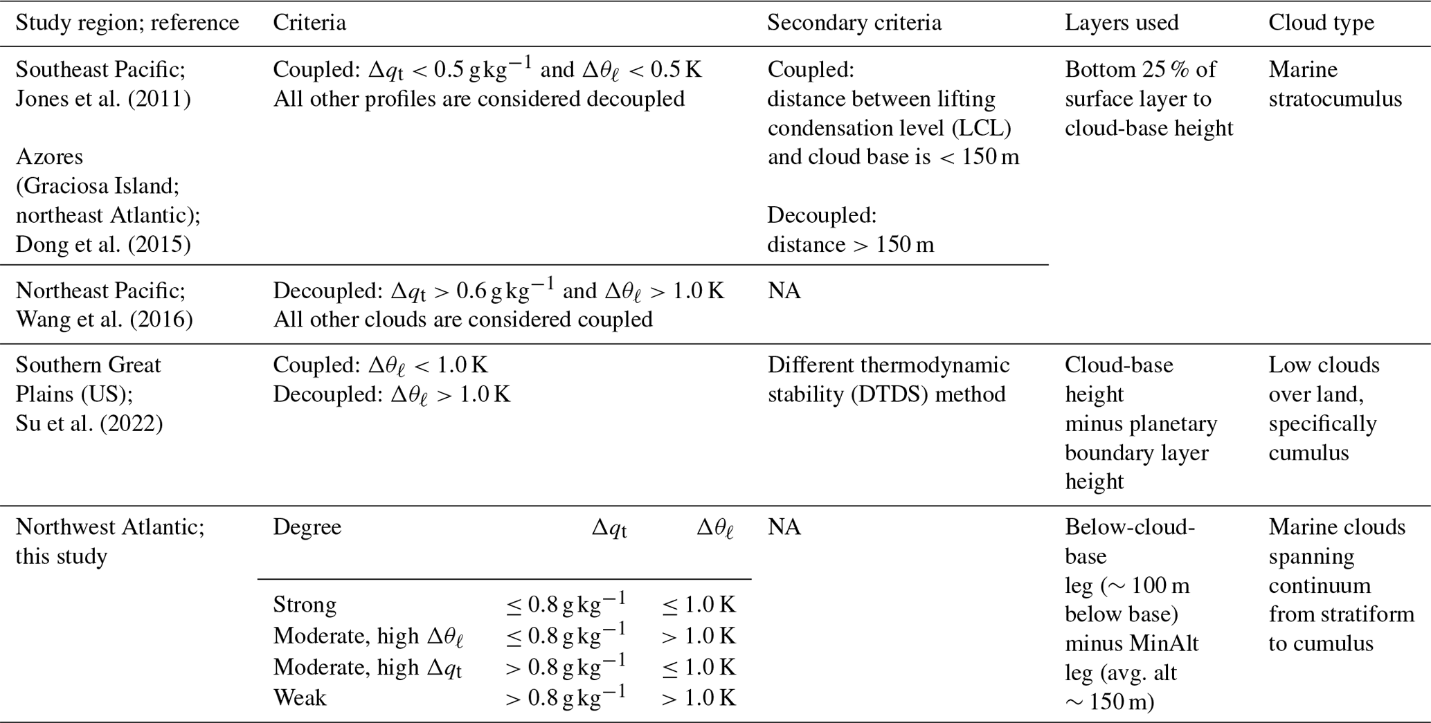
NA: not available.

As over 45 % of the ocean's surface is covered by MBL clouds (Warren et al., 1986), examining relations between aerosol and cloud characteristics with coupling strength is important. Investigation of coupling behavior has not yet been carried out for the northwest Atlantic region, which is a complex thermodynamic region for such work as it is not a classical subtropical zone with a stratocumulus cloud deck like most regions investigated in Table 1 (Painemal et al., 2021, 2023). The synoptic conditions over the northwest Atlantic are such that the wintertime has a higher cloud fraction with more influence from stratiform boundary layer clouds, whereas the summertime has more trans-Atlantic flow in addition to a lower cloud fraction, with higher sea surface temperatures promoting shallow cumulus clouds (Painemal et al., 2021). During winter, there is more offshore advection of continental air (Corral et al., 2021; Dadashazar et al., 2021), enhanced precipitation frequency (Painemal et al., 2021), and cold-air outbreaks (CAOs), in which cold air is advected across the Gulf Stream front, resulting in pronounced differences between air and sea surface temperatures (Brümmer, 1997; Papritz and Spengler, 2015; Seethala et al., 2021). CAOs are typically associated with strong turbulent mixing, leading to the deepening of the boundary layer (Dadashazar et al., 2021; Painemal et al., 2021; Papritz and Spengler, 2015; Tornow et al., 2022). During CAO events, surface wind convergence is driven by horizontal pressure and boundary layer height gradients, contributing to a statically unstable lower troposphere (Painemal et al., 2021; Seethala et al., 2021).

Motivated by meteorological differences between the northwest Atlantic and other regions in Table 1, the question arises as to whether it is restrictive to consider just the categories of coupled and decoupled clouds; instead, it may be instructive to consider more categories and that they all may have some degree of coupling ranging from weak to strong. This strategy is built from past reports suggesting that the use of the term “decoupled” may not be appropriate and that an MBL can be coupled even though it is poorly mixed (Stevens et al., 1998). The latter case can be viewed as weakly coupled due to episodic updraft-driven convection that is less efficient at mixing the MBL than is the case in well-mixed MBLs in which downdrafts associated with cloud-top radiative cooling couple the cloud and sub-cloud layers (Stevens et al., 1998). Thus, the perspective we embrace in this work is that low-level clouds (<2 km) can be viewed as always being coupled to sub-cloud layers but to varying degrees.

The goal of this study is to leverage an opportune aircraft dataset covering multiple seasons between 2020 and 2022 from NASA's Aerosol Cloud meTeorology Interactions oVer the western ATlantic Experiment (ACTIVATE; Sorooshian et al., 2019) to quantify the frequency of occurrence for four different coupling regimes and how aerosol and cloud characteristics vary between them. We emphasize that this study is different in nature from those in Table 1 in that we do not examine the vertical extent of the full cloudy boundary layer as rigorously but instead focus more on aerosol and cloud characteristics for different coupling regimes based on definitions limited to the vertical region below cloud bases. The analyses presented here are important for reasons such as knowing how well the aerosols near the surface level represent the aerosol just below cloud bases, with implications for the aerosols that largely govern the drop concentration budget. In Sect. 2 we summarize the measurements and methods, including criteria applied with traditionally used thermodynamic variables to differentiate between four coupling categories. In Sect. 3 we report results including the frequency of occurrence of the four coupling regimes and differences in aerosol properties (light scattering, number and volume concentration) and cloud microphysical properties (composition and droplet number concentration) between these categories to see how they compare to past studies for other regions. Although there are scarce previous reports of such findings (e.g., Dong et al., 2015; Wang et al., 2016), the central hypotheses are based on confirming what has been shown or implied in other regions, in that more strongly coupled cases will have (i) more vertical homogeneity in aerosol properties between the sub-cloud layer and closer to the ocean's surface, (ii) cloud composition reflecting significantly more sea salt influence (Wang et al., 2016), and (iii) higher cloud drop number concentration compared to weakly coupled cases (Dong et al., 2015). Differences identified in aerosol and cloud characteristics between these four coupling regimes are important to inform both future flight designs and data analysis research to account for thermodynamic profiles when examining aspects of aerosol and cloud microphysics when using either satellite, reanalysis, airborne, or ground-based datasets.

2 Data and methodology

2.1 Overview of ACTIVATE

ACTIVATE was largely based out of NASA Langley Research Center in Hampton, Virginia, and carried out research flights (RFs) with two spatially coordinated aircraft as part of six deployments in winter and summer months between 2020 and 2022, with extensive measurement and deployment details provided elsewhere (Sorooshian et al., 2023). Secondary bases were used for a subset of flights in 2022, including in Bermuda for June 2022. Winter and summer are broadly defined as including the months of November–April and May–September, respectively. The HU-25 Falcon flew level legs in, below, and above MBL clouds to collect in situ atmospheric state, aerosol, trace gas, and cloud measurements, while the high-flying King Air at ∼9 km launched dropsondes and carried out remote sensing. The focus of this work is data collected by the Falcon. Out of 179 total flights, 135 were used that offered data conducive to this study's analysis including having the Falcon conduct “statistical survey” flights with “cloud ensembles” (Fig. 1), along with several physical conditions satisfied as discussed in Sect. 2.5. During statistical survey flights, which accounted for 93 % of ACTIVATE's flights, the Falcon repeatedly flew a series of legs, with Fig. 1 visually depicting one such cloud ensemble whereby the plane flew the following legs in this nominal order: two pairs of legs below cloud base (BCB) and above cloud base (ACB) followed by a descent to the minimum altitude (MinAlt) possible (∼150 m above sea level) and then a subsequent slant ascent for a leg above cloud top (ACT) followed by a final leg below cloud top (BCT). Sometimes the legs were flown in a different order based on flight restrictions and cloud conditions. Separate ensembles flown in clear-air conditions are outside the scope of this work. Each leg duration was ∼3.3 min (equivalent to ∼24 km) with the Falcon flying at ∼120 m s⁻¹ (Dadashazar et al., 2022a). The vertical slant ascents and descents between level legs, especially down to MinAlt and up to ACT, were helpful in gathering vertically resolved information during ensembles.

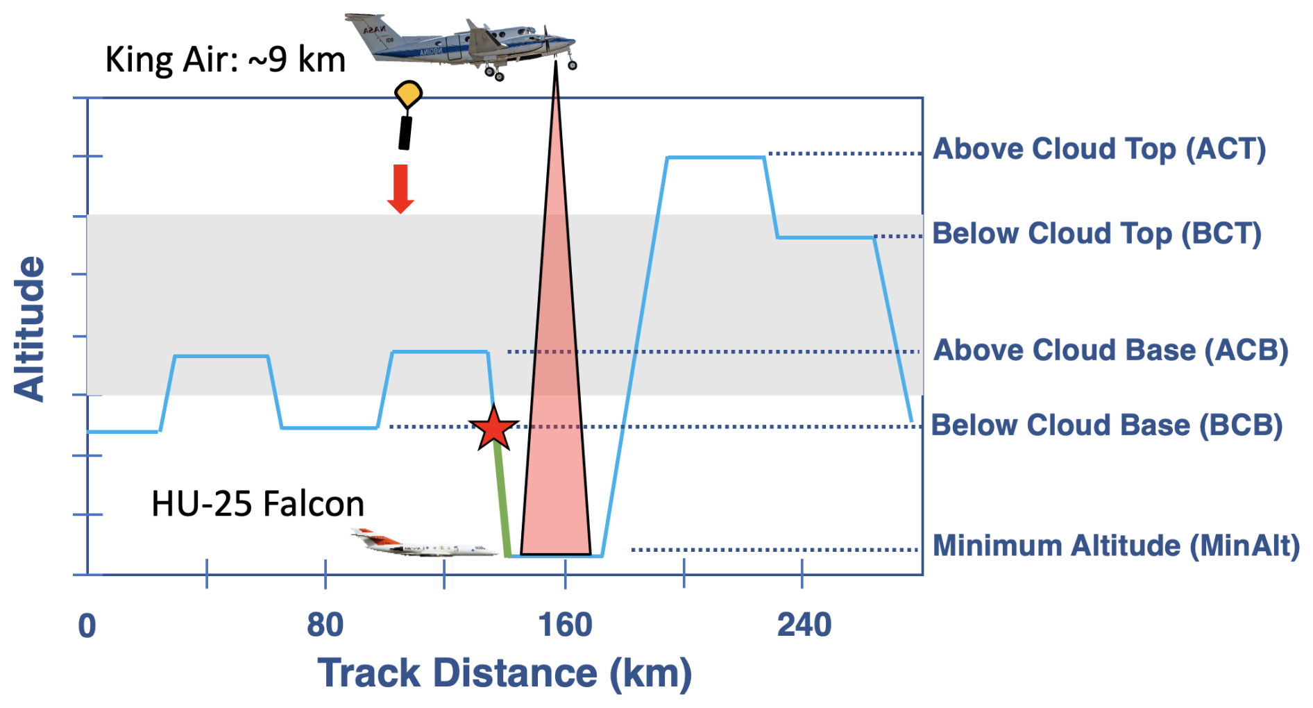
Figure 1 Cloudy ensemble flight strategy of the HU-25 Falcon during the ACTIVATE flights, where the gray box represents a typical cloud layer. The red star indicates where the BCB level would be marked and the data that would be utilized for this particular flight pattern. Otherwise, MinAlt–BCB pairs that are used include when a MinAlt level leg was immediately preceded or succeeded by a BCB level leg. The green line illustrates the data that would be used to investigate the vertical structure of the layer, starting with the last time stamp from the pseudo-BCB leg and ending with the first time stamp in the MinAlt leg.

2.2 Implementation of flight legs

Across ACTIVATE's six deployments, MinAlt and BCB legs were identified for RFs when the Falcon flew cloud ensembles (Fig. 1). There were several instances when the MinAlt and BCB legs were not immediately adjacent and separated by another leg, such as at ACB (i.e., the flight order was BCB, ACB, MinAlt; Fig. 1). In those cases, to get MinAlt–BCB pairs that were closer in time, our method involved identifying the BCB altitude during the slant altitudinal change (either descent or ascent) between MinAlt and ACB based on the altitude of the BCB leg immediately before the ACB leg (see red star in Fig. 1). A secondary check was made to ensure that the identified BCB leg was below cloud base using 1 Hz liquid water content (LWC) and N_d values from the fast cloud droplet probe (FCDP; criteria in Sect. 2.5). The vertical structure of the layer between MinAlt and BCB was examined using data between the last time stamp in the MinAlt and BCB leg (i.e., whichever was first in the MinAlt–BCB pair) and the first time stamp in the subsequent BCB and MinAlt leg (i.e., whichever was second in the MinAlt–BCB pair). This is indicated by a green line in Fig. 1, which begins with the last time stamp from the pseudo-BCB leg (indicated by the red star) and ends with the first time stamp in the MinAlt leg. For simplicity, we refer to the case of using BCB data during slant profiles as “legs” too, even though they were not level legs. This study compares various measurement data (Sect. 2.5) between MinAlt and BCB legs using the last and first 5 s of data during adjacent MinAlt–BCB legs, and in the case of slants, we use the two points before and after the actual BCB point (the red star in Fig. 1) for a total of five points (average altitude range ∼20 m) that represent the BCB level with the condition that all data were out of cloud.

2.3 Instrumentation

A summary of instrumentation relevant to this study is shown in Table 2 and briefly described here. A nephelometer (TSI-3563) measured the dry scattering coefficient at 550 nm (particle diameter (D_p)<5.0 µm for 2020 and D_p<1.0 µm for 2021 and 2022). A laser aerosol spectrometer (LAS; TSI-3340) measured aerosol size distributions ($\mathrm{0.1}<D_{\mathrm{p}}<\mathrm{5.0}$ µm), and here we use the integrated aerosol volume concentration data. A fast cloud droplet probe (FCDP; SPEC Inc.) measured liquid water content (LWC) and particle and cloud drop size distributions between 3 and 50 µm. A two-dimensional stereo (2D-S; SPEC Inc.; $\mathrm{25}<D_{\mathrm{p}}<\mathrm{1500}$ µm) probe provided LWC, liquid droplet effective diameter, and an ice flag, where the ice flag is equal to 1 if ice was detected (otherwise the variable is equal to 0). A diode laser hygrometer (DLH) measured the water vapor mixing ratio (q_v). A turbulent air motion measurement system (TAMMS) measured three-dimensional winds (Thornhill et al., 2003), and an axial cyclone cloud water collector (AC3) (Crosbie et al., 2018) collected cloud water samples by inertially separating droplets from the air stream. Collected cloud water samples were then analyzed post-flight with ion chromatography (IC) with operating conditions summarized elsewhere (Corral et al., 2022; Gonzalez et al., 2022). Section 2.6 describes the cloud water data in more detail.

Table 2 Summary of field campaign instrumentation used and corresponding measurements.

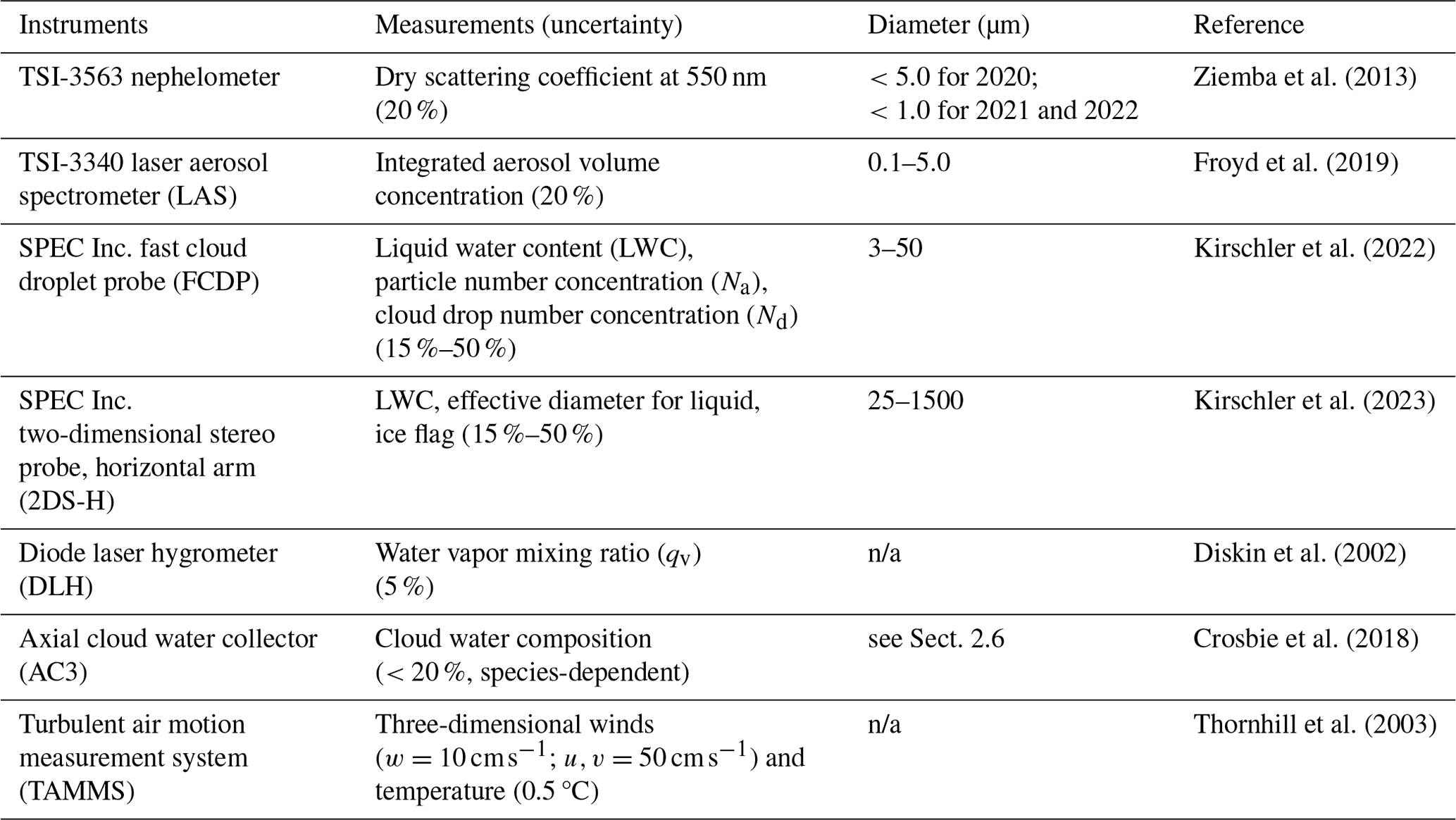
n/a: not applicable.

2.4 Marine boundary layer coupling

2.4.1 Thermodynamic variables

To estimate the degree of coupling within the marine boundary layer, we consider the change in vertical profile of two parameters: total water mixing ratio (q_t) and liquid water potential temperature (θ_ℓ). Relevant to this study are these equations:

$$\begin{array}{}\text{(1)}& {\displaystyle }{q}_{\mathrm{\ell }}={\displaystyle \frac{\text{LWC}}{{\mathit{\rho }}_{\mathrm{d}}}},\text{(2)}& {\displaystyle }{q}_{\mathrm{t}}=q_{\mathrm{v}}+q_{\mathrm{\ell }},\end{array}$$

where the total water mixing ratio is the sum of the water vapor mixing ratio (q_v) and liquid water mixing ratio (q_ℓ). The water vapor mixing ratio (q_v) provided by the DLH is converted from ppmv to g kg⁻¹. The liquid water mixing ratio (q_ℓ) is defined as the ratio of the mass of liquid water to the mass of dry air within a unit volume of air, which is equivalent to the ratio of LWC (provided by the FCDP) and the density of dry air (ρ_d).

Also relevant are these equations:

$$\begin{array}{}\text{(3)}& {\displaystyle }\mathit{\theta }=(T+\mathrm{273.15})\times {\left({\displaystyle \frac{p_{\mathrm{0}}}{p}}\right)}^{\mathit{\kappa }},\text{(4)}& {\displaystyle }{\mathit{\theta }}_{\mathrm{\ell }}=\mathit{\theta }-\left({\displaystyle \frac{L_{\mathrm{v}}}{c_{\text{pd}}}}\right)\times q_{\mathrm{\ell }},\end{array}$$

where in Eq. (3), T and p are the given temperature (°C) and pressure (hPa) from Falcon measurements, respectively, p₀ is the reference pressure (=1000 hPa), and κ is the ratio of the gas constant of dry air (R_d) to the specific heat of dry air at constant pressure (c_pd). In Eq. (4), L_v is latent heat of vaporization and c_pd is the specific heat of dry air at constant pressure. When LWC is equal to 0, θ_ℓ is equal to θ. θ_ℓ is useful for the purposes of this study as it is not significantly influenced by evaporating precipitation. Information regarding LWC thresholds for MinAlt–BCB pairs is included in Sect. 2.5.

For each MinAlt and BCB leg, the average θ_ℓ and q_t across the leg were calculated and the difference between the two layers was taken as follows:

$$\begin{array}{}\text{(5)}& {\displaystyle }\mathrm{\Delta }{q}_{\mathrm{t}}=q_{\text{t,MinAlt}}-q_{{\text{t,BCB}}^{\ast }},\text{(6)}& {\displaystyle }\mathrm{\Delta }{\mathit{\theta }}_{\mathrm{\ell }}={\mathit{\theta }}_{\mathrm{\ell },{\text{BCB}}^{\ast }}-{\mathit{\theta }}_{\mathrm{\ell },\text{MinAlt}},\end{array}$$

where in both Eqs. (5) and (6), the order of legs on the right-hand side is meant to arrive at a positive value for the difference based on expectation.

2.4.2 Coupling criteria

The criteria we use for the different coupling regimes were informed by (but are not identical to) those used in past work (Jones et al., 2011; Dong et al., 2015; Wang et al., 2016; Su et al., 2022). Our focus was on comparing the vertical range between MinAlt and BCB legs due to the focus on examining aerosol characteristics in particular within that range and also cloud microphysical conditions above cloud base. To qualify as strongly coupled, the difference between MinAlt and BCB had to satisfy these conditions: Δq_t≤0.8 g kg⁻¹ and Δθ_ℓ≤1.0 K (example in Fig. 2a). Since Δq_t is more influenced by evaporation and condensation, whereas Δθ_ℓ is more affected by air mass mixing (such as entrainment) and diabatic heating and cooling, it is proposed to have two degrees of moderate coupling – when Δq_t or Δθ_ℓ fit the strong coupling criteria and the other did not (Fig. 2b and c). Finally, profiles are considered “weakly coupled” when both Δq_t and Δθ_ℓ do not satisfy the strong coupling criteria values (Fig. 2d). Vertical profiles of q_t and θ_ℓ were examined for all MinAlt–BCB pairs to ensure robustness of the categorization method. As noted by Dadashazar et al. (2022b), the Falcon aimed to conduct BCB and ACB legs about ∼100 m below and above the estimated cloud-base height, respectively. Median and mean distances from BCB to cloud bases were as follows, respectively, for all samples in the four coupling categories: strong (73 and 87 m), moderate with high Δθ_ℓ (101 and 119 m), moderate with high Δq_t (69 and 71 m), and weak (104 and 142 m). The use of the two moderate categories is exploratory in nature and meant to identify whether differences are found between the two and between them and the more extreme categories of strong and weak. Appendix A further explores differences between the two moderate regimes and suggests that the moderately coupled category with high Δθ_ℓ is influenced more by processes above the MBL, such as entrainment of dry air with high potential temperature, whereas the other moderate category with high Δq_t is influenced by surface processes.

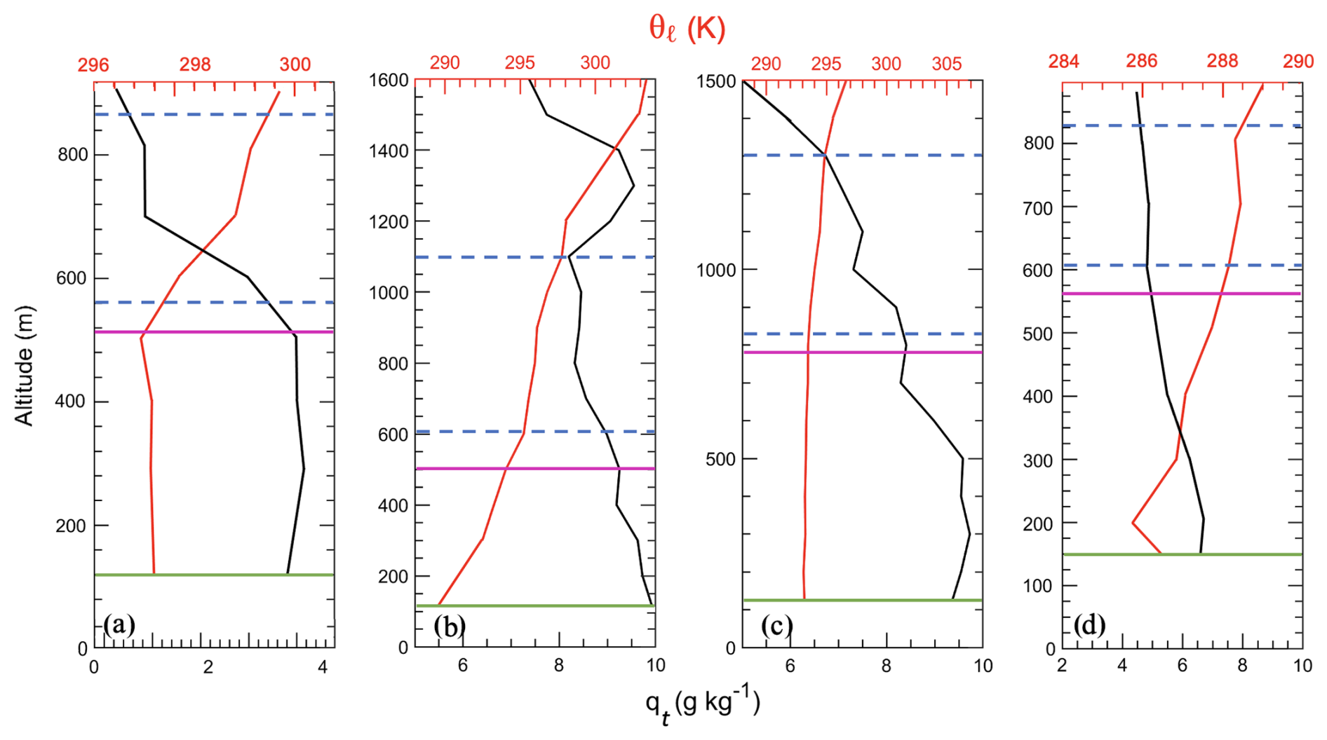
Figure 2 Representative vertical profiles of θ_ℓ and q_t for (a) strong coupling from RF 26 on 21 August 2020, (b) moderate coupling with high Δθ_ℓ from RF 150 on 5 May 2022, (c) moderate coupling with high Δq_t from RF 66 on 18 May 2021, and (d) weak coupling from RF 11 on 28 February 2020. The dashed blue lines demarcate the cloud-top and cloud-base levels, the magenta line indicates the BCB leg, and the green line indicates the MinAlt leg. A total of 411 MinAlt–BCB pairs were analyzed in this study.

2.5 Aerosol and atmospheric properties

There were several aerosol and atmospheric properties investigated in this study: aerosol scattering (scat) at 550 nm (<5 µm in 2020 and <1 µm in 2021–2022), integrated volume concentration (IntV: $\mathrm{0.1}<D_{\mathrm{p}}<\mathrm{5}$ µm), particle number concentration (N_a; $\mathrm{3}<D_{\mathrm{p}}<\mathrm{50}$ µm), cloud drop number concentration (N_d; $\mathrm{3}<D_{\mathrm{p}}<\mathrm{50}$ µm), and turbulence (σ_w). Note that the N_a measurement from the FCDP for diameter >3 µm is important in this study to better isolate sea salt particles (Gonzalez et al., 2022). The integrated volume concentration is also expected to be influenced by larger sea salt particles in the measurement size range. These properties were averaged across each MinAlt and BCB pair and the difference between the MinAlt and BCB values was computed. To account for interference from cloud droplet shatter with the aerosol statistics, we only looked at MinAlt–BCB pairs when the sampling area was devoid of cloud, rain, and ice. The following three criteria had to be met: (1) ice flag from 2DS-H of 0, (2) effective liquid diameter from 2DS-H<60 µm, and (3) LWC from FCDP<0.005 g m⁻³ to filter out conditions with ice, liquid precipitation, and clouds, respectively. When considering in-cloud conditions for N_d, additional criteria were needed based on FCDP data: LWC>0.05 g m⁻³ and N_d>10 cm⁻³ (Kirschler et al., 2023). N_d data were collected from ACB legs closest in proximity to a MinAlt–BCB pair (<30 min; 60 % within 10 min) due to one of the study objectives being to examine how N_d varies between the four defined coupling regimes. Turbulence was calculated as the standard deviation of the vertical wind velocity for a level leg as done in other work (e.g., MacDonald et al., 2020).

2.6 Cloud water species

The nine cloud water species of interest in this study include non-sea-salt calcium (nss Ca²⁺), chloride (Cl⁻), potassium (K⁺), magnesium (Mg²⁺), sodium (Na⁺), ammonium (${{\mathrm{NH}}_{\mathrm{4}}}^{+}$), nitrate (${{\mathrm{NO}}_{\mathrm{3}}}^{-}$), oxalate, and non-sea-salt sulfate (nss ${{\mathrm{SO}}_{\mathrm{4}}}^{\mathrm{2}-}$). Calculations of nss Ca²⁺ and nss ${{\mathrm{SO}}_{\mathrm{4}}}^{\mathrm{2}-}$ utilized mass ratios and concentrations of pure Ca²⁺, Na⁺, and ${{\mathrm{SO}}_{\mathrm{4}}}^{\mathrm{2}-}$, following the methodology outlined in Sect. 2.7 of AzadiAghdam et al. (2019). The IC is used to obtain concentrations of cloud water species in aqueous units (mg L⁻¹), which were then converted to air equivalent concentrations using the methods described in Gonzalez et al. (2022). Briefly, the cloud water sample was considered in-cloud under the criteria LWC_FCDP>0.05 g m⁻³. When this condition was met, the concentration was multiplied by the average LWC_FCDP measured across the sampling time and divided by the density of water and ultimately converted to µg m⁻³ for the air equivalent concentration. These units allow one to compare concentrations more fairly between samples to remove biases due to varying amounts of water in different clouds. As cloud water samples were collected periodically during flights, samples were only examined when a MinAlt or BCB leg being investigated was within 30 min of or overlapped with the collection period. Out of a total of 535 cloud water samples over the six deployments, 67 met the criteria to be used for this study's MinAlt–BCB pairs. Statistics including the mean, standard deviation (SD), minimum, maximum, and quartile ranges were calculated across the 67 data points for all nine cloud water species.

Additionally, cumulative average cloud water mass concentrations and mass fractions were calculated for the 67 samples. The total mass concentration for each coupling regime was found by the summation of only the nine chemical species investigated in this paper. Welch's t-test calculations were conducted to compare the mean concentrations of the investigated chemical species across coupling regimes. These tests were done in lieu of the traditional t test due to the assumption that the data used have unequal variances and are thus slightly more robust.

3 Results and discussion

3.1 Thermodynamic criteria

This section discusses the application of the developed thermodynamic criteria across all MinAlt–BCB pairs. In total, 411 MinAlt–BCB pairs were investigated (pair locations shown in Fig. 3; the MinAlt legs were close in time to the BCB legs, so only one spatial map is needed to show the approximate data point location for each pair), with the breakdown of the distribution across the different degrees of coupling shown in Figs. 3 and 4. The majority of the pairs were classified as strongly coupled, with a breakdown of 71 % (strongly coupled), 14 % (moderately coupled with high Δθ_ℓ), 10 % (moderately coupled with high Δq_t), and 5 % (weakly coupled). Strong turbulent mixing in the northwest Atlantic Ocean, especially during the winter (Brunke et al., 2022), which is when most pairs were identified, is likely why the majority of pairs were found to be strongly coupled, as the coupling parameters θ_ℓ and q_t are relatively constant vertically from the surface to near cloud bases due to the strong mixing (Fig. 2a).

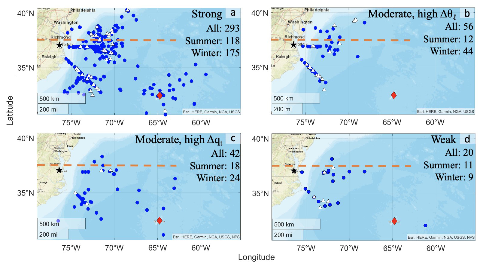
Figure 3 Locations of the BCB segments of the MinAlt–BCB pairs (blue circles), broken up into the four different degrees of coupling. The locations of the cloud water samples (white triangles) are overlaid on the BCB segment locations. The black star indicates the location of NASA Langley Research Center, the red diamond indicates Bermuda, and the dashed orange line indicates 37.5° N, which is referenced in the discussion about this figure. The total number of MinAlt–BCB pairs for each category is also included for each coupling regime.

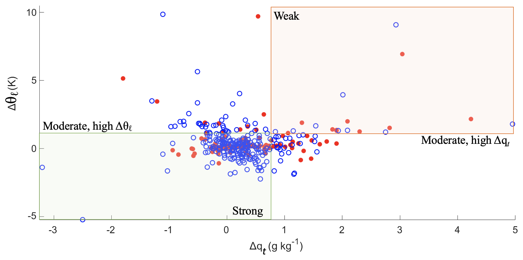
Figure 4 Scatterplot of Δθ_ℓ vs. Δq_t values for the BCB and MinAlt pairs divided into the four coupling regimes, where winter pairs are indicated by blue points and summer pairs are indicated by red points. Refer to Fig. 3 for the number of points in each coupling regime categorized by season. Figure S1 in the Supplement shows this information in the form of a joint frequency histogram.

There are no major spatial distribution differences for MinAlt–BCB pairs across the four coupling regimes with minor exceptions being that the majority of pairs identified farther offshore around Bermuda were for both the strongly coupled and moderately coupled with high Δq_t categories. Also, the strong and moderate coupling with high Δθ_ℓ categories had more pairs north of 37.5° N (indicated by the dashed orange line), which coincides with more wintertime sampling of cold-air outbreak events that feature turbulent conditions (e.g., Painemal et al., 2021; Kirschler et al., 2022).

Figures 3 and 4 show that were more MinAlt–BCB pairs during the winter versus summer (252 vs. 159), largely due to the greater ease of sampling such cases with the higher wintertime cloud fraction in the region (Painemal et al., 2021; Kirschler et al., 2022, 2023). But generally, the distribution of coupling categories was the same (summer and winter): 74 % and 70 % strongly coupled, 8 % and 18 % moderately coupled with high Δθ_ℓ, 11 % and 10 % moderately coupled with high Δq_t, and 7 % and 4 % weakly coupled. The frequency of the moderately coupled with high Δq_t category was relatively higher in summer versus winter compared to the other moderate category, which is coincident with the summer having higher temperatures (i.e., higher q_v) and more flights farther south in Fig. 3 where temperatures are warmer compared to farther north.

For context, applying the criteria from past work in Table 1 (Jones et al., 2011; Dong et al., 2015) to this dataset (i.e., Δq_t [g kg⁻¹] and Δθ_ℓ [K]<0.5 for coupled and all others decoupled) would have led to 206 and 205 coupled and decoupled cases, respectively, with a seasonal breakdown as follows (summer and winter): 43 % and 58 % coupled, 35 % and 66 % decoupled. However, we caution that the compared vertical levels differ between these studies. For example, Jones et al. (2011) compared levels encompassing more of the full extent of the cloudy MBL (e.g., somewhat analogous to the use of MinAlt and BCT in Fig. 1), whereas in this study we compare MinAlt to BCB due to our focus on aerosol characteristics, which are difficult to measure in clouds. While ACTIVATE flights were designed for achieving a statistically rich dataset portraying the region in an unbiased way, the frequency of occurrence of the four coupling regimes in this study can possibly still be affected by how flights were designed to fly towards areas with a relatively higher cloud fraction without complicating scenes such as those with multiple cloud layers. We also note that sensitivity tests were conducted (Table S1 in the Supplement) to see how the assignment of MinAlt–BCB pairs to the four coupling categories changed when accounting for measurement uncertainties (shown in Table 2), which could push points across the border of their regime in Fig. 4. Varying Δq_t and Δθ_ℓ by absolute values of 0.2 in both directions was investigated to test for sensitivity to measurement uncertainty in this study. Results are preserved with only slight changes in assignments after varying the criteria; the same applies using the Jones et al. (2011) criteria, shown on the far right of Table S1. Subsequent effects on other results presented in the following sections were minimal with the same general conclusions reached.

3.2 Aerosol and atmospheric properties

The results of the aerosol and atmospheric parameter calculations across the four different coupling regimes are provided in Table 3 (seasonal results in Tables S2 and S3 in the Supplement), with notched box plots summarizing information from Table 3 in Fig. S2 in the Supplement. Of the 411 MinAlt–BCB pairs, 293 were used in aerosol calculations after eliminating pairs that may have been influenced by rain, cloud, or ice interference. As a note, when quantifying altitudinal differences in variables across different coupling regimes, the mean at each altitude is used as the comparison parameter unless otherwise stated, as outliers were already removed prior to data analysis.

The first hypothesis of this study is that strongly coupled regimes would have greater turbulence (σ_w) than weakly coupled regimes. This hypothesis is confirmed when examining σ_w results at both MinAlt (strong and weak are indicated by 0.86 and 0.55 m s⁻¹) and BCB levels (strong and weak are indicated by 0.70 and 0.49 m s⁻¹). The two categories of moderate coupling had greater turbulence at both altitudes compared to weak coupling and sometimes had greater turbulence than pairs categorized as strongly coupled. Further, while BCB σ_w and BCB–MinAlt σ_w had no significant differences across medians, there were some significant differences across coupling regimes for MinAlt σ_w (Fig. S2). Data in the moderate with high Δθ_ℓ coupling regime were significantly different from the other regimes, and data categorized as moderate coupling with high Δq_t were also statistically distinct from the weak coupling regime. This suggests that considering multiple coupling regimes for the northwest Atlantic is important to tease out such nuances as differences in the thermodynamic profiles can potentially coincide with different aerosol and cloud characteristics as discussed subsequently.

Table 3 Statistics for various atmospheric properties investigated across the MinAlt–BCB pairs (Δ calculation refers to the MinAlt value minus the BCB value), except for MinAlt σ_w and BCB σ_w, which are the average σ_w for each respective leg, and for N_d, which is calculated in ACB legs. Each property is broken down into the different degrees of coupling (n is the number of points used in each coupling category). Variable acronyms are defined in Sect. 2.5. Refer to Fig. S2 for corresponding notched box plots.

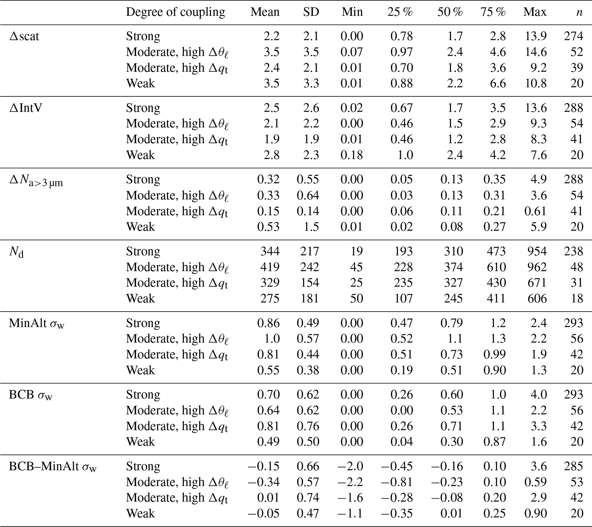
The second hypothesis is that aerosol scattering (Δscat), integrated volume concentration ($\mathrm{0.1}<D_{\mathrm{p}}<\mathrm{5}$ µm; ΔIntV), and giant particle number concentration ($\mathrm{3}<D_{\mathrm{p}}<\mathrm{50}$ µm; ΔN_>3 µm) would have more vertically homogenous concentrations (i.e., smaller MinAlt–BCB differences) in strongly coupled regimes compared to weakly coupled regimes due to greater mixing for the former as supported by the higher σ_w results already shown. This hypothesis is supported (Table 3 and Fig. S2) since strong coupling cases exhibited lower mean differences (MinAlt–BCB) than weak coupling (Δscat: 2.2 and 3.5 Mm⁻¹, ΔIntV: 2.5 and 2.8 µm³ cm⁻³, and ΔN_>3 µm: 0.3 and 0.5 cm⁻³ for strong and weak regimes). The third hypothesis was that cloud drop number concentration ($\mathrm{3}<D_{\mathrm{p}}<\mathrm{50}$ µm; N_d) would be greater in strong coupling conditions, as stronger updrafts and turbulence would help to activate more particles into cloud droplets (this was also found in Dong et al., 2015). This is confirmed in Table 3: mean N_d is 344 and 275 cm⁻³ for strong and weak regimes for ACB legs coinciding with each MinAlt–BCB pair. This result is consistent with past studies for the northwest Atlantic linking stronger turbulence to greater droplet activation efficiency (Kirschler et al., 2022; Dadashazar et al., 2021). The results based on medians agree with those of mean values in Table 3, although medians across regimes for each atmospheric property were not statistically different from one another (Fig. S2). Although there is a lack of statistically significant differences between the four coupling regimes for the investigated atmospheric properties, it is important to note that the sample sizes for each regime vary greatly. Therefore, there is more variability within the weak coupling regime with only 20 data points compared to the strong coupling regime with over 200 data points. As this study utilized all of the data at its disposal and there were more strong coupling cases than any other coupling regime, the lack of statistical significance across coupling regimes did not impact the general conclusions of the study.

When comparing the moderate coupling regimes with the strong and weak regimes, neither Δscat, ΔIntV, nor ΔN_>3 µm showed a consistent trend in terms of being higher or lower across all three variables. However, one consistent feature among the moderate regimes is that the moderate with high Δq_t category showed smaller Δ values than moderate with high Δθ_ℓ for the three aerosol variables. Sometimes, the lowest Δ values did not occur during the strong coupling cases but rather during moderate coupling with high Δq_t cases (i.e., ΔIntV=1.9 µm³ cm⁻³, $\mathrm{\Delta }{N}_{>\mathrm{3}\mathrm{\mu }\mathrm{m}}=\mathrm{0.2}$ cm⁻³). These low differences should presumably coincide with the highest values of σ_w. This is somewhat supported by how BCB σ_w was greatest for the moderate coupling with high Δq_t regime (0.81 ± 0.76 m s⁻¹), although MinAlt σ_w was greatest for the moderate coupling with high Δθ_ℓ regime (1.00 ± 0.57 m s⁻¹), with the value for the moderate coupling with high Δq_t regime being 0.81 ± 0.44 m s⁻¹. Also, Appendix A provides a discussion in support of why the high Δq_t category may have small aerosol differences between MinAlt and BCB levels, whereby surface effects may be at play to help promote mixing in the MBL. Interestingly, the highest N_d values were for the moderate with high Δθ_ℓ category with a mean of 419 cm⁻³, which can partly be explained by how most of these cases occurred during the winter flights when N_d is higher than in the summer (see also Tables S2 and S3) due to strong updraft velocities that efficiently activate particles into droplets (e.g., Kirschler et al., 2022). These conditions in winter were common during cold-air outbreaks (Dadashazar et al., 2021).

3.3 Cloud water species

A total of 67 cloud water samples were used in this study (Table 4), with 60 % of the samples falling into the strong coupling regime, followed by moderate coupling with high Δθ_ℓ (25 %), weak coupling (9 %), and lastly moderate coupling with high Δq_t (6 %). Locations of samples are shown in Fig. 3. Within the strong coupling and moderate coupling with high Δθ_ℓ categories, there were several samples north of 37.5° N (marked by orange line in Fig. 3), whereas the moderate coupling with high Δq_t and weak coupling samples were all south of that latitude. The former two categories include substantially more data during the winter when air masses typically come from the continent featuring urban emissions (Dadashazar et al., 2022a).

Table 4 Average cloud water mass concentrations (µg m⁻³) and mass fractions (in %, rounded to the nearest whole number) for all cloud water samples. Also shown are the pH and ${\mathrm{Cl}}^{-}:{\mathrm{Na}}^{+}$ mass ratios. Results are categorized into different degrees of coupling, and the ratio of weak-to-strong coupling is also reported.

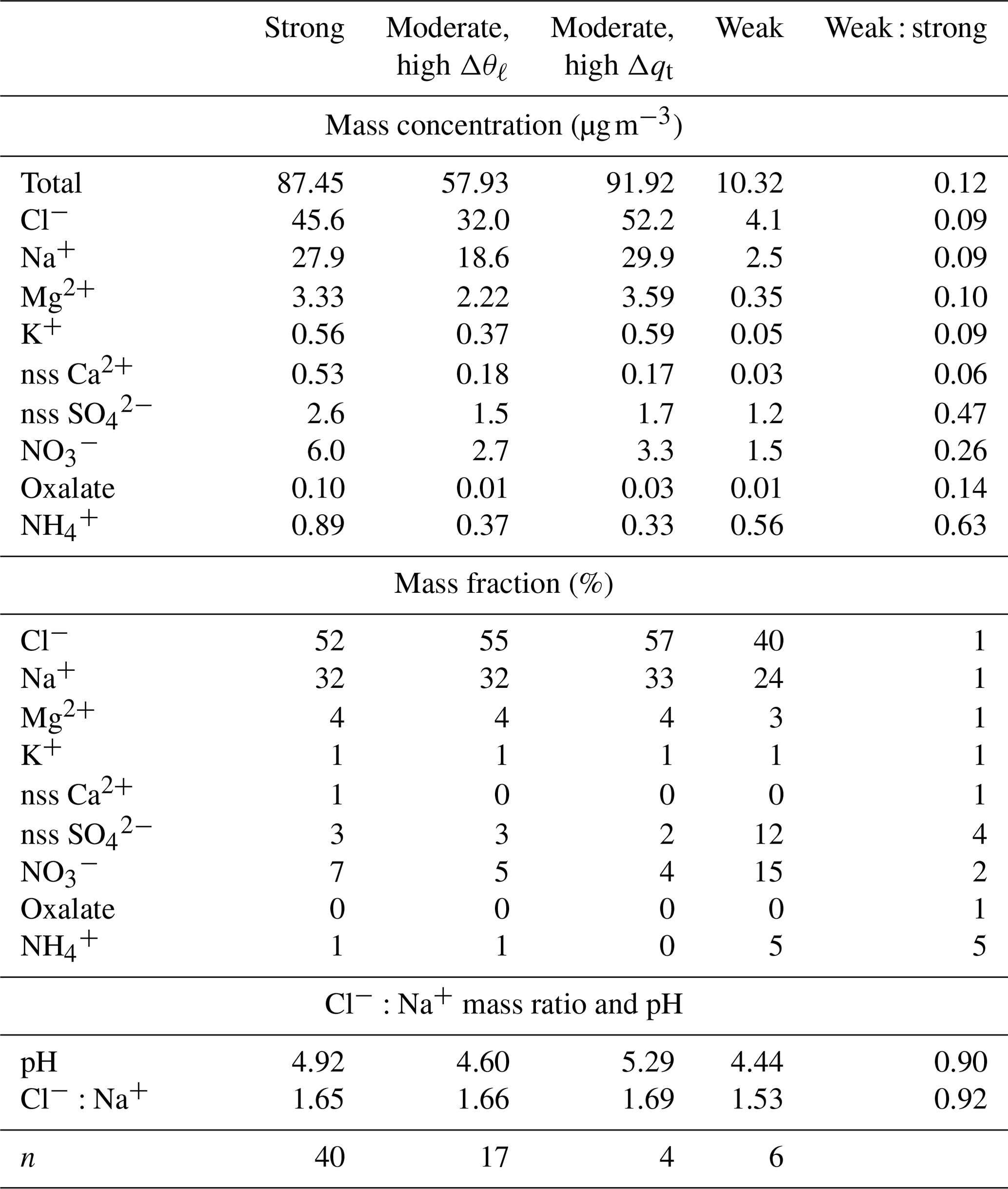
Figure 5 provides composition statistics for the cloud water samples categorized into the four coupling regimes. As a note, the notches of the box plots assist in the determination of statistical significance between multiple medians (the shading indicates where the notches begin and end). If notches or shading do not overlap, the medians are statistically different from one another (also referred to as statistically significant). Since this study has utilized means instead of medians when comparing values across coupling regimes, mean concentrations are provided in the Supplement (Tables S4–S6 in the Supplement) and the results of Welch's t tests for each category (mean cloud water concentrations of the nine chemical species, pH, and ${\mathrm{Cl}}^{-}:{\mathrm{Na}}^{+}$) are given in Table S7 in the Supplement. This study also investigated cumulative average mass concentrations and mass fractions (Table 4) to paint a clearer picture of the breakdown of chemical species for different degrees of coupling. Based on previous work for stratocumulus clouds over the northeast Pacific (Wang et al., 2016), we hypothesized that samples from strong coupling regimes would have higher mass concentrations compared to weakly coupled regimes owing to higher concentrations of sea salt constituents (e.g., Cl⁻, Na⁺, Mg⁺, and K⁺). More turbulent conditions in strongly coupled cases are thought to promote more mixing of sea salt into boundary layer clouds, which can be detected with cloud water composition measurements (e.g., Dadashazar et al., 2017).

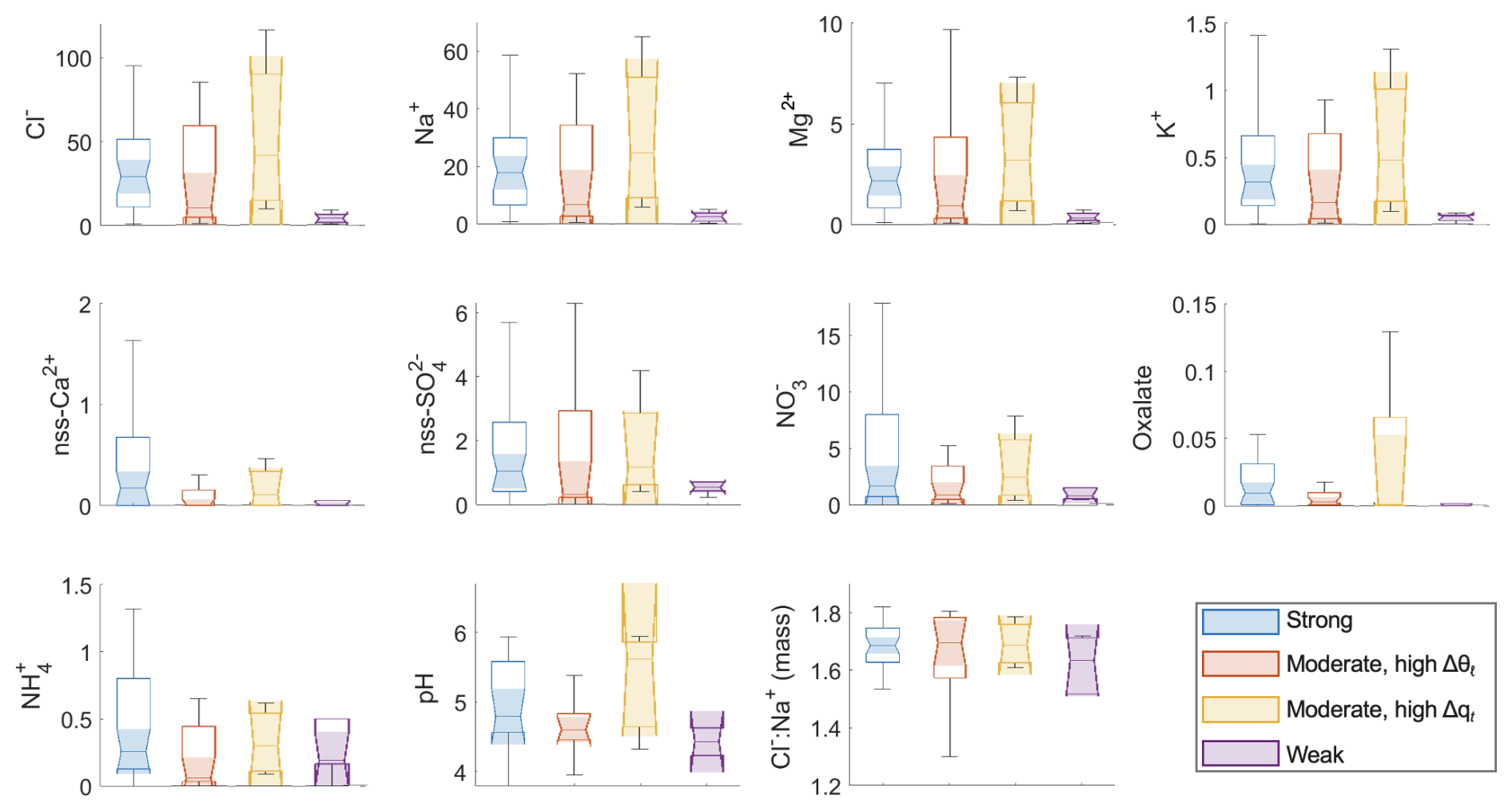
Figure 5 Notched box plots of species concentrations (µg m⁻³), ${\mathrm{Cl}}^{-}:{\mathrm{Na}}^{+}$ mass ratio, and pH from cloud water samples collected during periods coinciding with MinAlt–BCB pairs.

Strong coupling regime samples exhibit higher average mass concentrations compared to weak coupling, and Na⁺, Cl⁻, K⁺, and ${{\mathrm{NO}}_{\mathrm{3}}}^{-}$ were all found to be statistically different across the two regimes (p values: $\mathrm{1.07}\times {\mathrm{10}}^{-\mathrm{4}}$, $\mathrm{3.54}\times {\mathrm{10}}^{-\mathrm{5}}$, $\mathrm{5.52}\times {\mathrm{10}}^{-\mathrm{5}}$, and $\mathrm{9.57}\times {\mathrm{10}}^{-\mathrm{3}}$, respectively). The most abundant species by mass across the coupling regimes were usually Cl⁻, Na⁺, and ${{\mathrm{NO}}_{\mathrm{3}}}^{-}$, similar to the results of Wang et al. (2016). Further, although lower in absolute mass concentration, some species were relatively more abundant (i.e., higher mass fraction) in the weak coupling regime: nss ${{\mathrm{SO}}_{\mathrm{4}}}^{\mathrm{2}-}$ (12 % – weak vs. 3 % – strong), ${{\mathrm{NO}}_{\mathrm{3}}}^{-}$ (15 % – weak vs. 7 % – strong), and ${{\mathrm{NH}}_{\mathrm{4}}}^{+}$ (5 % – weak vs. 1 % – strong). Oxalate was very low in overall concentration and exhibited comparable mass fractions. These results are consistent with the idea of surface emissions (mainly sea salt) driving cloud water composition in turbulent conditions (i.e., strongly coupled) in contrast to weakly coupled clouds that have much lower overall mass concentrations of the reported ions but relatively more influence from non-sea-salt species. The two moderate coupling regimes include samples with concentration and mass fraction values more similar to the strongly coupled regime, with even higher sea salt tracer species concentrations for the moderate with high Δq_t regime. This is consistent with the aerosol results in Sect. 3.2 suggesting that this latter category can have an appreciable influence from the surface, although it is also important to note that this is based on four cloud water samples.

Wang et al. (2016) analyzed 35 cloud water constituents for northeast Pacific stratocumulus clouds and found that 27 chemical species were higher in coupled clouds, with the remaining eight (acetate, formate, Si, ${{\mathrm{NO}}_{\mathrm{2}}}^{-}$, Al, Mn, Cr, and Co) higher in decoupled clouds due to relatively more continental influence. The 27 cloud water species that were higher in coupled clouds were associated with a mix of anthropogenic and natural sources (i.e., sea salt emissions for Cl⁻ and Na⁺). Conversely, the eight species that were higher in decoupled clouds were associated with crustal matter and biogenic sources. Several of the most abundant species from our study (Na⁺, Cl⁻, Mg²⁺) are common sea salt tracers, while ${{\mathrm{NO}}_{\mathrm{3}}}^{-}$ sources in the region may include ocean sea spray and biogenic emissions, wildfires, agricultural emissions, and ship exhaust (Corral et al., 2020, 2021, 2022; Shah et al., 2018). Note that nitric acid can partition effectively into cloud droplets as well, which can drive up cloud water ${{\mathrm{NO}}_{\mathrm{3}}}^{-}$ levels (e.g., Prabhakar et al., 2014). At least some of the species with higher mass fractions in the weakly coupled regime (e.g., nss ${{\mathrm{SO}}_{\mathrm{4}}}^{\mathrm{2}-}$, ${{\mathrm{NO}}_{\mathrm{3}}}^{-}$) have previously been linked to combustion sources in this region, such as industrial emissions and transportation (Brock et al., 2008; Song et al., 2001). Ammonium is a major base forming salts with nss ${{\mathrm{SO}}_{\mathrm{4}}}^{\mathrm{2}-}$ and ${{\mathrm{NO}}_{\mathrm{3}}}^{-}$, whereas oxalate has diverse sources (e.g., continental, marine) and can be associated with sea salt and produced via cloud processing (e.g., Stahl et al., 2020; Hilario et al., 2021). Nss Ca²⁺ is often associated with continental crustal matter (Ma et al., 2021; Edwards et al., 2024), and its concentrations are generally very low, suggestive of a low influence from dust during the majority of ACTIVATE flights.

In addition to examining mass concentrations, we also examined pH and ${\mathrm{Cl}}^{-}:{\mathrm{Na}}^{+}$. Regarding the latter ratio, sea salt chloride concentrations can be reduced in the presence of acidic species such as sulfuric and nitric acids (e.g., Braun et al., 2017; Edwards et al., 2024). This phenomenon is known as Cl⁻ depletion, and it can be calculated by taking the ratio of ${\mathrm{Cl}}^{-}:{\mathrm{Na}}^{+}$. For context, Wang et al. (2016) reported no major difference in the ${\mathrm{Cl}}^{-}:{\mathrm{Na}}^{+}$ ratio in cloud water over the northeast Pacific but measured lower pH in coupled clouds (4.26) versus decoupled clouds (4.48). In this study, samples in the weak coupling regime exhibited the lowest pH (4.4 vs. 5.0 for strong coupling) and ${\mathrm{Cl}}^{-}:{\mathrm{Na}}^{+}$ (1.5 vs. 1.7 for strong coupling), which could potentially be related to the higher relative amount of nss ${{\mathrm{SO}}_{\mathrm{4}}}^{\mathrm{2}-}$ and ${{\mathrm{NO}}_{\mathrm{3}}}^{-}$. The two moderate coupling regimes feature samples with pH and ${\mathrm{Cl}}^{-}:{\mathrm{Na}}^{+}$ values more similar to strongly coupled samples.

A limitation in this analysis is that there were only six cloud water samples that fell into the weak coupling regime. Future work examining the sensitivity of aerosol and cloud characteristics to coupling regimes should try to obtain better sampling coverage across all regimes.

4 Conclusions

This study used data collected during the NASA ACTIVATE mission (2020–2022) from the HU-25 Falcon to assess the frequency of different degrees of MBL cloud coupling and also how aerosol and cloud characteristics varied among four such regimes. MinAlt and BCB legs were used to assess thermodynamic statistics along with turbulence, aerosol, and cloud variables, which were calculated at each leg, and the differences of the two legs were taken for final comparison metrics. Cloud water species and N_d values associated with MinAlt and BCB pairs were analyzed when cloud sampling occurred within 30 min of a MinAlt–BCB pair.

Vertical profiles between MinAlt and BCB pairs were divided into four degrees of coupling: strongly coupled (Δq_t≤0.8 g kg⁻¹, Δθ_ℓ≤1.0 K), moderately coupled with high Δθ_ℓ (Δq_t≤0.8 g kg⁻¹, Δθ_ℓ>1.0 K), moderately coupled with high Δq_t (Δq_t>0.8 g kg⁻¹, Δθ_ℓ≤1.0 K), and weakly coupled (Δq_t>0.8 g kg⁻¹, Δθ_ℓ>1.0 K). In total, 411 MinAlt–BCB pairs were investigated, along with 67 cloud water samples. Using this coupling categorization criteria, only a handful of weakly coupled MBL clouds were detected (20, compared to 286 with strong coupling). The relative amounts of the regimes did not vary substantially between the winter and summer seasons. Instead, particular focus was placed on comparing regimes with strong coupling to those with weak coupling. Support for the coupling criteria was sought through five different aerosol, cloud, and dynamic parameters (Δscat, ΔIntV, ΔN_>3 µm, N_d, and σ_w) and 11 cloud water variables (nss Ca²⁺, Cl⁻, K⁺, Mg²⁺, Na⁺, ${{\mathrm{NH}}_{\mathrm{4}}}^{+}$, ${{\mathrm{NO}}_{\mathrm{3}}}^{-}$, oxalate, nss ${{\mathrm{SO}}_{\mathrm{4}}}^{\mathrm{2}-}$, pH, ${\mathrm{Cl}}^{-}:{\mathrm{Na}}^{+}$). Turbulence was generally greater during regimes of strong coupling compared to weak coupling, which corresponded to lower values of Δscat, ΔIntV, and ΔN_>3 µm due to better presumed mixing in the MBL. N_d was higher for strong coupling regimes, as higher turbulence likely encouraged more cloud drop activation, which was also observed in Dong et al. (2015) for the northeast Atlantic. Sea salt tracers (e.g., Na⁺, Cl⁻, and K⁺) were higher in concentration in strongly coupled compared to weakly coupled MBL clouds and were found to have statistically significant differences across the two coupling regimes. Additionally, nss ${{\mathrm{SO}}_{\mathrm{4}}}^{\mathrm{2}-}$, ${{\mathrm{NO}}_{\mathrm{3}}}^{-}$, and ${{\mathrm{NH}}_{\mathrm{4}}}^{+}$, which are linked to continental sources, were found in higher mass fractions during weak coupling regimes; this was also observed in Wang et al. (2016) for northeast Pacific stratocumulus clouds, corresponding to lower values of both cloud water pH and the ${\mathrm{Cl}}^{-}:{\mathrm{Na}}^{+}$ ratio.

The inclusion of two moderate coupling categories is shown to be insightful as differences between the two can potentially be explained by the relative influence of subsidence and entrainment versus surface effects. More specifically, the moderately coupled category with high Δθ_ℓ is thought to be influenced more by processes above the MBL, such as entrainment of dry air with high potential temperature, whereas the other moderate category with high Δq_t likely has more influence from surface processes. These speculations are supported by how the moderate with high Δq_t regime exhibited even more turbulent mixing than the strong coupling regime, yielding the highest sea salt concentrations in cloud water and the lowest values of ΔIntV and ΔN_>3 µm. Furthermore, the moderate with high Δθ_ℓ category exhibited the highest mean N_d value (419 cm⁻³) of any category (275–344 cm⁻³ for the other three categories), which can be partly explained by how most of these cases (44 of 56) were in winter flights when N_d is typically higher than summer, especially during cold-air outbreaks (e.g., Dadashazar et al., 2021).

This study is the first to our knowledge to investigate degrees of coupling in MBL clouds through thermodynamic statistics in the northwest Atlantic with a focus on aerosol and cloud microphysical characteristics. Further research of this nature is needed in other regions to assess thermodynamic criteria for MBL cloud to surface coupling, including how aerosol and cloud characteristics change with degrees of MBL coupling in different regions. The results here indicate that a failure to account for different coupling regimes can mix together varying aerosol and cloud microphysical characteristics in data analysis studies, which increases risk of separating out important details such as how cloud composition is very different across the spectrum of cloud coupling strength. A limitation of this study to build on is obtaining more statistics for the more weakly coupled category, which in part may be influenced by how flight plans are designed. The results of this research have important implications for studies of aerosol–cloud interactions; not considering coupling strength will make interpretations difficult, as we have shown important differences for aerosol and cloud properties.

Appendix A: Discussion of the two moderate regimes

To help with the interpretation of the two moderate regimes defined in Table 1, we provide a perspective based on the following discussion. Using Eq. (1) but expanding it to take the difference of the liquid water potential temperature between the BCB and MinAlt flight legs yields the following.

$$\begin{array}{}\text{(A1)}& {\displaystyle }\begin{array}{rl}{\displaystyle }\mathrm{\Delta }{\mathit{\theta }}_{\mathrm{\ell }}=& {\displaystyle }\left({\mathit{\theta }}_{\text{BCB}}-\left({\displaystyle \frac{L_{\mathrm{v}}}{c_{\text{pd}}}}\right)\times q_{\mathrm{\ell },\text{BCB}}\right)\\ {\displaystyle }& {\displaystyle }-\left({\mathit{\theta }}_{\text{MinAlt}}-\left({\displaystyle \frac{L_{\mathrm{v}}}{c_{\text{pd}}}}\right)\times q_{\mathrm{\ell },\text{MinAlt}}\right)\end{array}\end{array}$$

Note that both q_ℓ terms are small below cloud. The Δθ_ℓ value can thus be large due to large-scale subsidence or entrainment when dry air from the free troposphere with high θ is potentially mixed with air at the BCB level. While θ_MinAlt can be high due to surface heating, it acts to reduce Δθ_ℓ. Also, the current MinAlt is slightly above the typical surface layer and hence the surface inversion. Also, note that

$$\begin{array}{}\text{(A2)}& \mathrm{\Delta }{q}_{\mathrm{t}}=(q_{\text{v,MinAlt}}+q_{\mathrm{\ell },\text{MinAlt}})-(q_{\text{v,BCB}}+q_{\mathrm{\ell },\text{BCB}}),\end{array}$$

where both q_ℓ terms are small below cloud and are typically much smaller than q_v. The range of q_v is largely controlled by the temperature due to the Clapeyron–Clausius equation (the higher temperature, the higher saturation vapor pressure). While high Δq_t may be due to low q_v at the BCB level, it is more likely due to high q_v near the surface because saturation vapor pressure exponentially increases with temperature.

To conclude, the Δθ_ℓ term is more likely influenced by features above the MBL, while the Δq_t term is more likely influenced by near-surface effects.