The importance of moist thermodynamics on neutral buoyancy height for plumes from anthropogenic sources

Plume rise plays a critical role in dispersing pollutants emitted from tall stacks, dictating the height reached by buoyant plumes and their subsequent downwind dispersion. Commonly, plume rise is assumed to be governed by atmospheric stability and by the exit momentum and temperature of the effluent released from large stacks. However, an under-recognized influence on plume rise is the effects of entrained and/or co-emitted water, which can change the plume height due to exchange of latent heat associated with phase changes in within-plume water. While many of the stack sources achieve high temperatures of the emitted effluent via combustion, the impact of combustion-generated water on plume rise is often overlooked in large-scale air quality models. As the rising water condenses or evaporates, it releases or absorbs latent heat, influencing the height reached by the plumes. Our study investigates the effects of latent heat exchange by combustion-generated and entrained water on plume rise. We introduce a novel approach that integrates moist thermodynamics into an empirical parameterization for plume rise, resulting in the development of PRISM (Plume-Rise-Iterative-Stratified-Moist). Long-term (6-month duration) simulations using PRISM exhibit a difference of up to ±100 % in surface concentrations of emitted pollutants near industrial sources compared to previous predictions, emphasizing the substantial influence of moist thermodynamics on plume rise. Our results show up to 50 % improvement in model-simulated plume height through evaluation vs. aircraft observations over the Canadian oil sands. This study pioneers a plume rise sub-grid parameterization integrating moist thermodynamics in iterative calculation of neutral buoyancy height for plumes emitted from industrial stacks, thereby advancing our understanding of plume behaviour and enhancing the accuracy of air quality modelling. These advancements can potentially contribute to more effective pollution control strategies.

1 Introduction

Effluents emitted from industrial and urban sources (e.g. stacks) are often much warmer than the surrounding air and are therefore buoyant. If the source of heat for the effluent is the combustion of hydrocarbons, in which water is a by-product of combustion, then the water content of the rising plume may be greater than that of the surrounding atmosphere. The emitted effluents rise to higher altitudes than the original release height due to exit momentum and buoyancy, while the water vapour content simultaneously condenses (as plumes expand and cool), forming the visible (cloud-like) plumes that can be observed rising from chimney stacks and other sources (e.g. Sturman and Zawar-Reza, 2011). The buoyant rise due to the effluent's exit velocity and temperature upon emissions is captured within standard algorithms for plume rise (e.g. Briggs, 1984). However, the effects of latent heat exchange due to water condensation into droplets and evaporation of these droplets for plumes emitted from industrial stacks have not been implemented as a controlling variable in plume rise sub-grid parameterization in air quality models. Through 3D numerical modelling of the governing processes (e.g. mass and energy balance), Gangoiti et al. (1997) have shown the impact of latent heat exchange on plume buoyancy and atmospheric dispersion for plumes from tall stacks. However, computational costs prevent the use of explicit numerical modelling of plume trajectory for regional large-scale air quality models with grid sizes of a few kilometres and domain sizes of thousands of kilometres, where plumes from thousands of simultaneously emitting sources may be simulated. For these regional chemical transport models (e.g. Community Multiscale Air quality (CMAQ) or Global Environmental Multiscale – Modelling Air quality and Chemistry (GEM-MACH)), plume rise is usually determined using some form of sub-grid parameterization embedded within the host 3D model (e.g. Briggs, 1984). We note that latent heat effects have been previously taken into account in plume rise parameterization for vegetation (wild)fires (e.g. Freitas et al., 2007; Chen et al., 2019). However, sub-grid parameterizations in large-scale air quality (chemical transport) models commonly do not incorporate moist thermodynamics when estimating plume rise from high-temperature industrial stacks. The transport of the emitted pollutants is governed by meteorological conditions and atmospheric flow regimes (wind speed and direction) at the effective release height. Therefore, to reliably predict the range/extent of the atmospheric dispersion of the emitted pollutants, accurate plume rise parameterization is essential and has important implications for air quality predictions. For instance, determining the final plume rise (sometimes referred to as the effective stack height) is a requirement for the estimation of the maximum surface concentration at distances downwind of the emission source. Calculating the final rise with acceptable certainty is more difficult for unstable (convective) conditions where turbulence is the main rise-limiting factor (the rise may never actually terminate) compared to stable atmosphere conditions with low winds (Briggs, 1984). Since the 1960s, a large amount of research work has been dedicated to plume rise parameterization through dimensional analysis, where empirical parameters are determined from laboratory measurements and field observations (Hoult et al., 1969). Many air quality models (e.g. Im et al., 2015; Byun and Ching, 1999; Holmes and Morawska, 2006) use a variation of the empirical formulations developed by Gary A. Briggs during late 1960s to early 1980s (e.g. Briggs, 1965, 1969, 1975, 1984), such as the Community Multiscale Air Quality (CMAQ; Byun and Schere, 2006) and Global Environmental Multiscale – Modelling Air quality and Chemistry (GEM-MACH; Moran et al., 2010) models. Briggs (1984)' empirical formulations parameterize plume rise based on estimates of meteorological conditions (e.g. stability) at the stack location/height, source information (e.g. stack flow rate, temperature), estimated entrainment rates, and observed plume height data. Briggs' formulations (and most other plume rise parameterizations) assume uniform meteorological conditions (e.g. temperature, wind speed) over the vertical span of the plume, either taken at the stack top or averaged over the atmospheric layers between the bottom and top of the plume. Such simplifications, when applied to cases where the atmospheric vertical structure is complex, can lead to large errors in plume final-rise estimation. While commonly employed, subsequent evaluations of such parameterizations have shown over/underpredictions by over 50 % vs. observed plume heights (e.g. Hamilton, 1967; England et al., 1976; Rittmann, 1982; Webster and Thomson, 2002). Gordon et al. (2018) conducted extensive evaluations of plume rise prediction using the Briggs (1984) formulation driven by ambient observations vs. aircraft SO₂ measurements over the Canadian oil sands (OS) during the Joint Oil Sands Monitoring (JOSM) 2013 campaign (ECCC, 2018). They found that the Briggs (1984) plume rise algorithm significantly underpredicted the observed SO₂ plume heights, with more than 50 % of the predicted plume heights less than half that of observed heights for plumes from large SO₂-emitting OS sources. Results by Gordon et al. (2018) also included a subset of cases (less than 12 %) with overpredicted plume heights, where plume height predictions by the Briggs (1984) algorithm were more than twice the observed SO₂ plume heights. These discrepancies were partially attributed to potential presence of spatial heterogeneity in the meteorological data used to drive the plume rise algorithm (input data were not co-located with the emission stacks). The impact of spatial heterogeneity was confirmed by Akingunola et al. (2018) through high-resolution meteorological model simulations for the same locations and time periods. Akingunola et al. (2018) demonstrated, using model-generated meteorological conditions at stack locations and calculations of residual plume buoyancy at successive levels above the inversion layer height, that incorporation of these factors into a plume rise model can significantly improve plume rise predictions, with 70 % of predictions falling within a factor of 2 of the observed plume heights.

Utilizing more accurate source emissions information (e.g. continuous emission monitoring systems (CEMSs)) and source-specific meteorology can improve the confidence in initial/input information for plume rise parameterization, while a layered approach can better resolve plume buoyancy in cases of more complex atmospheric conditions. However, efforts to improve plume rise parameterization (for large-scale air quality models) have largely ignored the potential importance of (within-plume) water thermodynamic effects. Plume buoyancy is commonly determined in terms of initial stack exit temperature and buoyancy flux reduction as the plume rises, along with estimates of the ambient temperature gradient (i.e. the height at which the plume comes to rest, having the same density as the ambient atmosphere). However, as we show in the following work, release and/or uptake of the latent heat associated with phase changes in water can potentially alter plume buoyancy enough to impact the plume rise significantly. In this work, we introduce a new plume rise algorithm that performs plume buoyancy calculations at all vertical levels above the stack top (as opposed to Akingunola et al., 2018, where plume residual buoyancy calculations are done only above the inversion layer height), which also accounts for the effect of latent heat exchange associated with phase changes in within-plume water content. This algorithm expands on relevant concepts from Briggs (1984) and Akingunola et al. (2018) while including estimates of water emissions (due to combustion) from stack sources in a new plume rise parameterization. Following comparisons of predicted plume heights using an observation-driven model (offline/standalone simulations with the new plume rise model) vs. observed heights, we implemented the new parameterization within the GEM-MACH air quality model (Moran et al., 2010; Makar et al., 2021) and conducted a series of retrospective air quality model simulations for the Athabasca oil sands (OS) region. We considered a simulation period that overlaps with that of a 2018 aircraft measurement campaign over OS as part of the Canada–Alberta oil sands monitoring program (OSM; ECCC, 2018). We conducted sensitivity analyses on the plume rise parameterization and evaluated model performance vs. surface monitoring data and aircraft measurements.

2 Methods

2.1 PRISM (Plume-Rise-Iterative-Stratified-Moist): the new algorithm for plume rise parameterization

We developed a plume rise prediction algorithm based on effluent buoyancy flux reduction while accounting for thermodynamic effects associated with latent heat release/uptake as described below. The stack parameters such as stack radius, exit momentum, and temperature are translated into effluent initial conditions (i.e. volume flux, temperature, density). The initial water vapour content ($m_{{\mathrm{H}}_{\mathrm{2}}\mathrm{O},\mathrm{stack}}$ [kg]) in the effluent is determined from annual and/or hourly emission rate inventory data for water vapour. The (known) input stack parameters also include the stack top height z_stack in metres above ground level [m a.g.l.], stack radius r_stack [m], stack volume flow rate ${\dot{V}}_{\mathrm{stack}}$ [m³ s⁻¹], stack/effluent temperature T_stack [K], and effluent exit velocity w_stack [m s⁻¹]. The effluent buoyancy is determined in relation to ambient air information, which can be from sounding data or model-generated ambient state variables. The buoyancy flux immediately above the stack top (F₀) is then calculated as the product of effluent buoyant acceleration and the stack volume flow rate (${\dot{V}}_{\mathrm{stack}}$),

$$\begin{array}{}\text{(1)}& F_{\mathrm{0}}=g{\displaystyle \frac{{\mathit{\rho }}_{\mathrm{air}}-{\mathit{\rho }}_{\mathrm{stack}}}{{\mathit{\rho }}_{\mathrm{stack}}}}{\dot{V}}_{\mathrm{stack}},\end{array}$$

where g [m s⁻²] is the gravitational acceleration, ρ_air [kg m⁻³] is ambient air density, and ρ_stack [kg m⁻³] is effluent (dry air) density at the stack top (see Supplement, Sect. S1, Eqs. S1 to S6 for the derivations and the corresponding discrete formulations).

Briggs (1984) noted that the behaviour of plumes under low-wind-speed conditions differed from that in higher wind speeds and described these two conditions with two different equations, one for “vertical” and the other for “bent-over” plumes. Vertical plumes occur when the buoyancy and momentum of the emitted gases are strong enough (and/or the wind speeds are sufficiently low) to overcome the effects of wind. This typically happens under stable atmospheric conditions or when the stack emissions are significantly hotter and faster than the surrounding air. The plume rises vertically under these conditions until it reaches the neutral buoyancy height, where the plume parcel density approaches the ambient air density. Bent-over plumes, on the other hand, occur when the wind speed is strong enough to bend the plume horizontally. This is more common under neutral or unstable atmospheric conditions. The plume initially rises due to its buoyancy and momentum but is then bent over by the wind, creating a trajectory that is more horizontal than vertical. The parcel volume flux as it rises through the plume (which includes the effects of entrainment), $\dot{V}$ [m³ s⁻¹], is determined based on empirical formulations for buoyant plumes by Briggs (1984):

$$\begin{array}{}\text{(2)}& \dot{V}\left(z\right)=\left\{\begin{array}{ll}\mathrm{0.791}{\mathit{\alpha }}^{\mathrm{4}/\mathrm{3}}{F}_{\mathrm{0}}^{\mathrm{1}/\mathrm{3}}{z}^{\prime \mathrm{5}/\mathrm{3}},& \text{vertical},\\ \mathit{\pi }U\left(z\right){\mathit{\beta }}^{\mathrm{2}}{z}^{\prime \mathrm{2}},& \text{bent over},\end{array}\right.\end{array}$$

where $z^{\prime }=z-z_{\mathrm{stack}}$ is the height above the stack top [m], U [m s⁻¹] is the horizontal wind speed at z [m], and α and β are (dimensionless) empirical coefficients of entrainment (see Sect. S1, Eq. S7 for the corresponding discrete formulation). The Briggs (1984) formulation made use of the Taylor entrainment hypothesis: “the rate at which ambient air is drawn into the plume is proportional to the velocity shear between the plume and the ambient fluid, and this shear consists mainly of the plume's vertical velocity”. Briggs (1984) recommended (empirical) entrainment coefficients of about α=0.08 and β=0.6 for buoyant plumes. The change in effluent plume volume between two adjacent atmospheric heights can be calculated by multiplying the average volume flux by the transit time between those heights as it rises, $\mathrm{\Delta }V\left(z\right)=\stackrel{\mathrm{‾}}{\dot{V}}\left(z\right)\mathrm{\Delta }t$. The transit time Δt [s] can be determined kinematically from parcel vertical velocity and buoyant acceleration at height z. Parcel volume V [m³], vertical velocity w [m s⁻¹], density ρ [kg m⁻³], temperature T [K], and buoyant acceleration a [m s⁻²] are numerically calculated in the algorithm for each consecutive vertical level z (derivations of the formulae presented here are provided in Sect. S1; see Eqs. S8 to S19). Using these updated parameters, the equivalent vapour pressure of the net amount of water in the parcel is calculated as

$$\begin{array}{}\text{(3)}& e_{\mathrm{v}}\left(z\right)={\displaystyle \frac{P_{\mathrm{a}}}{\mathit{\epsilon }}}{q}_{\mathrm{v}}={\displaystyle \frac{P_{\mathrm{a}}}{\mathit{\epsilon }}}\left({\displaystyle \frac{m_{{\mathrm{H}}_{\mathrm{2}}\mathrm{O}}}{\mathit{\rho }V}}\right),\end{array}$$

where q_v [kg kg⁻¹] is vapour mixing ratio, P_a [Pa] is air pressure (equivalent for ambient and parcel air), and ε=0.622 (Rogers and Yau, 1989). From Iribarne and Godson (1981), the saturation vapour pressure of water [Pa] as a function of temperature of the rising parcel T [K] is given by

$$\begin{array}{}\text{(4)}& e_{\mathrm{sat}}\left(T\right)={\mathrm{10}}^{\left[-\mathrm{2937.4}/T-\mathrm{4.9283}{\log }_{\mathrm{10}}T+\mathrm{25.5471}\right]}.\end{array}$$

In the following, we use simple parcel model parameterizations to estimate the latent heat release/uptake based on the approach described in Rogers and Yau (1989). If the parcel temperature drops below the saturation temperature at a given level, the amount of the water mass mixing ratio present in the condensed phase can be derived from the excess vapour pressure above saturation,

$$\begin{array}{}\text{(5)}& q_{\mathrm{c}}=max\left[\left(e_{\mathrm{v}}-e_{\mathrm{sat}}\left(T\right)\right){\displaystyle \frac{\mathit{\epsilon }}{P_{\mathrm{a}}}},\mathrm{0.0}\right].\end{array}$$

Note that q_c can be calculated at each model layer using the total water in the parcel and that an increase in q_c between two adjacent levels representing the layer midpoints implies that condensation of water mass has occurred between those levels, while a decrease in q_c implies that the evaporation of water mass has occurred between the levels. The corresponding release or uptake of latent heat can be calculated as

$$\begin{array}{}\text{(6)}& \mathrm{\Delta }{Q}_{\mathrm{cond}}=L_{\mathrm{v}}\mathrm{\Delta }\left(\mathit{\rho }V{q}_{\mathrm{c}}\right),\end{array}$$

where L_v is the latent heat of condensation. Further, the first law of thermodynamics (at constant pressure ΔP=0) may be used to determine the change in parcel temperature ΔT_cond resulting from the phase change in water (Rogers and Yau, 1989),

$$\begin{array}{}\text{(7)}& \mathrm{\Delta }{T}_{\mathrm{cond}}={\displaystyle \frac{\mathrm{\Delta }{Q}_{\mathrm{cond}}}{M{C}_p}},\end{array}$$

where C_p=1004 J kg⁻¹ K⁻¹ is the specific heat at constant pressure, and M=ρ V is the total parcel mass.

As in Briggs (1984), the rate of increase in the volume of the rising air parcel carrying the pollutants is assumed to be solely due to turbulent mixing between the parcel and the surrounding atmosphere (entrainment), in which case the change in parcel volume with respect to height can be used to estimate the change in mass due to entrainment: Δm_en(z)=(ρ_air(z)ΔV(z)) [kg], where the subscript “air” indicates the ambient outside-of-plume conditions at the given height. When the effluent is at a higher temperature than added ambient air mass (i.e. for buoyant plumes T>T_air), heat is transferred from the effluent to the entrained air,

$$\begin{array}{}\text{(8)}& \mathrm{\Delta }{Q}_{\mathrm{en}}\left(z\right)=-C_p\left(T-T_{\mathrm{air}}\right)\mathrm{\Delta }{m}_{\mathrm{en}}\left(z\right),\end{array}$$

resulting in a corresponding change (decrease) in parcel temperature,

$$\begin{array}{}\text{(9)}& \mathrm{\Delta }{T}_{\mathrm{en}}={\displaystyle \frac{\mathrm{\Delta }{Q}_{\mathrm{en}}}{M{C}_p}}.\end{array}$$

Another consideration with regard to entrainment is that the parcel may be rising through air that contains water, in both gaseous (q_v,a) and liquid (q_c,a) form, and this water may be entrained during the rise between vertical levels,

$$\begin{array}{}\text{(10)}& \mathrm{\Delta }{m}_{{\mathrm{H}}_{\mathrm{2}}\mathrm{O}}\left(z\right)=q_{*}\mathrm{\Delta }{m}_{\mathrm{en}}\left(z\right),\end{array}$$

where $q_{*}=q_{\mathrm{v},\mathrm{a}}+q_{\mathrm{c},\mathrm{a}}$ is the total entrained water content mixing ratio. The entrained water contributes to the total water within the plume: $m_{{\mathrm{H}}_{\mathrm{2}}\mathrm{O}}+\mathrm{\Delta }{m}_{{\mathrm{H}}_{\mathrm{2}}\mathrm{O}}$ (with the stack-emitted water $m_{{\mathrm{H}}_{\mathrm{2}}\mathrm{O},\mathrm{stack}}$ as the initial value). The entrained water can influence parcel condensation or evaporation through adding or removing mass from the condensed phase. If we assume all the water content within the parcel to be vapour, the equivalent vapour pressure of the new net amount of water in the parcel can be recalculated from Eq. (3). The revised value of e_v can then be used to determine the new value of the condensed-phase water within the parcel q_c from Eq. (5). Referring back to Eq. (6), the energy lost or gained due to the entrained water added to the parcel will be de facto included in the heat exchange included in the equation.

The moist plume rise algorithm is stratified in the sense that it performs layered calculations for plume vertical momentum, state variables, and buoyancy. At each height, the amount of entrained air and water is determined. Further, the change in temperature as a result of heat transfer to the entrained air and latent heat release/uptake (due to phase changes in water) is determined. The contributing processes can be summarized as follows:

$$\begin{array}{}\text{(11)}& \begin{array}{rl}\mathrm{\Delta }T\left(z\right)& =\mathrm{\Delta }{T}_{\mathrm{cond}}\left(z\right)+\mathrm{\Delta }{T}_{\mathrm{en}}\left(z\right)\\ & ={\displaystyle \frac{\mathrm{1}}{M{C}_p}}\left[\mathrm{\Delta }{Q}_{\mathrm{cond}}\left(z\right)+\mathrm{\Delta }{Q}_{\mathrm{en}}\left(z\right)\right],\end{array}\end{array}$$

where positive (negative) values of ΔT indicate increases (decreases) in plume temperature.

The algorithm utilizes an iterative solver (Newton–Raphson/secant method; Oxford, 2014) to calculate parcel temperature, executing several iterations (up to a user-defined maximum iteration number; for our tests, 20 to 50 iterations were sufficient) until it converges on a solution for the (equilibrium) parcel temperature at a given layer in the atmosphere. The parcel density is then recalculated from the ideal gas law as a function of the revised parcel temperature and air pressure,

$$\begin{array}{}\text{(12)}& \mathit{\rho }\left(z\right)={\displaystyle \frac{P_{\mathrm{a}}\left(z\right)}{k{T}_{\mathrm{v}}\left(z\right)}},\end{array}$$

where water mixing ratios in the vapour q_v(z) and condensed q_c(z) phases are accounted for in calculating the updated parcel density in the virtual temperature term,

$$\begin{array}{}\text{(13)}& \begin{array}{rl}{T}_{\mathrm{v}}\left(z\right)& =T\left(z\right)\left[{\displaystyle \frac{\mathrm{1}+q_{\mathrm{v}}\left(z\right)/\mathit{\epsilon }}{\mathrm{1}+q_{\mathrm{v}}\left(z\right)}}-q_{\mathrm{c}}\left(z\right)\right]\\ & \approx T\left(z\right)\left(\mathrm{1}+\mathrm{0.61}{q}_{\mathrm{v}}\left(z\right)-q_{\mathrm{c}}\left(z\right)\right).\end{array}\end{array}$$

Note that the addition of condensed water further modifies parcel buoyancy (see chap. 3 of Stull, 2017). The updated parcel density is then compared to ambient air density. If the solution results in positive buoyancy (that is, the parcel density is still below that of the ambient air), the plume continues to rise to the next vertical level up. These layered calculations are repeated up to the vertical level at which the plume buoyancy is either zero or negative (ρ(z)≥ρ_air(z)). The height of this vertical level is then taken as the final plume height. Finally, the plume vertical spread is determined from the plume rise above the stack height Δh, and the emitted mass is uniformly distributed in the vertical between the plume bottom and top, determined following the commonly used method from Briggs (1975),

$$\begin{array}{}\text{(14)}& \begin{array}{rl}{h}_{\mathrm{t}}=& h_{\mathrm{s}}+\mathrm{1.5}\mathrm{\Delta }h,\\ h_{\mathrm{b}}=& h_{\mathrm{s}}+\mathrm{0.5}\mathrm{\Delta }h,\end{array}\end{array}$$

where h_s, h_t, and h_b are the stack top, plume top, and plume bottom heights, respectively.

Our new plume rise algorithm PRISM (Plume-Rise-Iterative-Stratified-Moist) is essentially a 1D model (with user-defined resolutions and parameters) that can be run as a standalone model or embedded within a host 3D model (in this case GEM-MACH) as a sub-grid parameterization scheme. In Sect. 3 we discuss results from both standalone simulations and GEM-MACH model runs. PRISM takes stack parameters (e.g. volume flow rate, temperature, water content) and ambient air state variables as input information and performs high-resolution (high vertical resolution) layered calculations of parcel-buoyancy-driven rise. At each height, the algorithm calculates the change in parcel temperature (and corresponding change in density) as it rises, expands, and mixes with the ambient air, while taking into account the effects of latent heat uptake/release due to phase changes in within-parcel water content. Note that the release or absorption of latent heat due to condensation or evaporation of water in the parcel may serve to decrease or increase parcel buoyancy, depending on ambient conditions such as the temperature profile and ambient water content. See Sect. S1 for algorithm details and the corresponding discrete numerical formulations.

2.2 Model description and setup

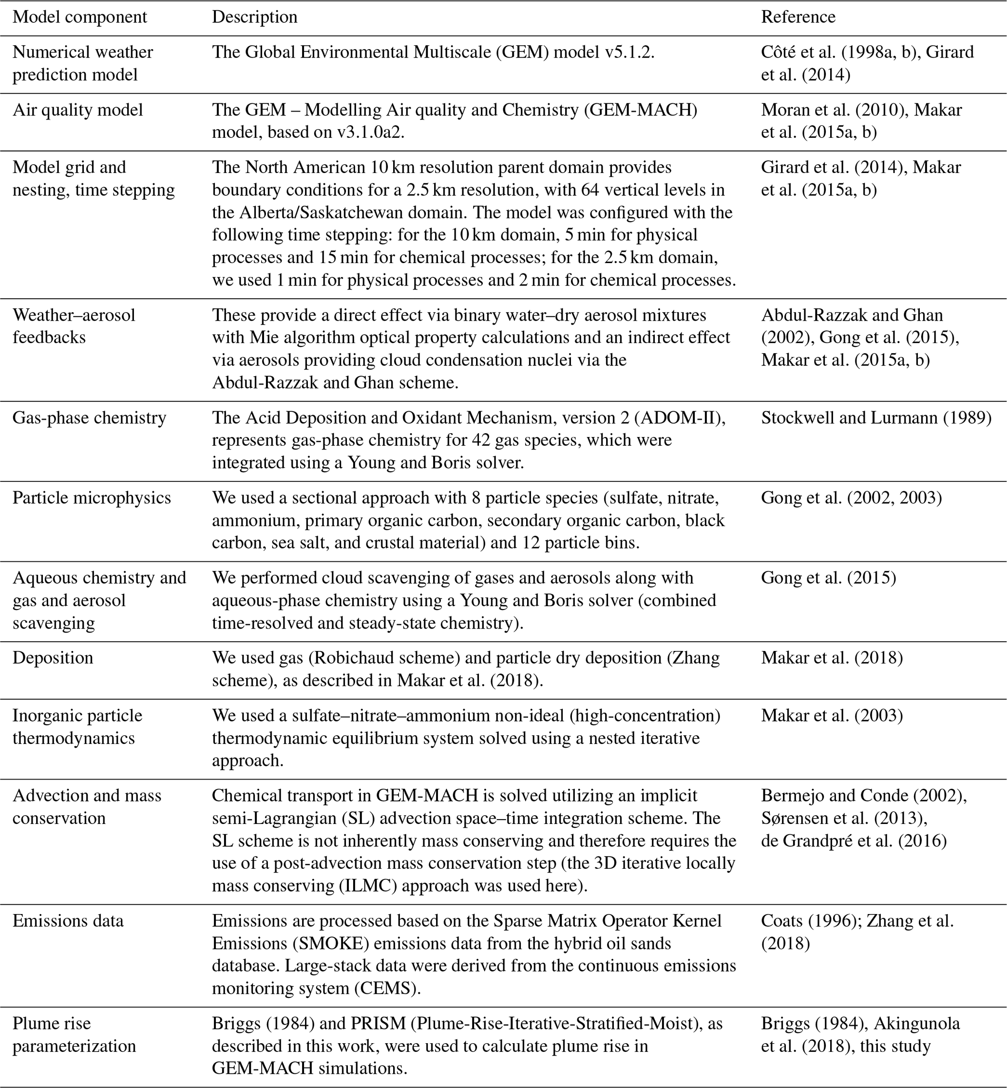
The Global Environmental Multiscale – Modelling Air quality and Chemistry (GEM-MACH) model is Environment and Climate Change Canada's (ECCC) air quality prediction model (Moran et al., 2010). GEM-MACH is an online air quality and chemical transport model, which resides within the Global Environmental Multiscale (GEM) numerical weather prediction model (Côté et al., 1998a, b; Girard et al., 2014). The GEM meteorological model and its components have been extensively evaluated elsewhere in the literature (e.g. Côté et al., 1998b; Bélair et al., 2003b, a; Li and Barker, 2005; Milbrandt and Yau, 2005a, b; Fillion et al., 2010; Girard et al., 2014; Milbrandt and Morrison, 2016). In addition to the GEM weather prediction model, GEM-MACH includes an atmospheric chemistry module (Moran et al., 2010) with gas and particle process representation. GEM-MACH is used here in its fully coupled configuration – i.e. the model's particulate matter is allowed to modify the meteorological predictions through direct and indirect aerosol effects (Makar et al., 2015a, b; Gong et al., 2015). For a recent evaluation of GEM-MACH's performance, see Makar et al. (2021); also see Fathi et al. (2021) for a comprehensive discussion of tracer mass budget and transport in GEM-MACH. For this work, a nested configuration for GEM-MACH was used, with a parent domain covering North America at a 10 km resolution and a nested high-resolution domain with a 2.5 km grid spacing over the Canadian provinces of Alberta and Saskatchewan, including the Athabasca oil sands region (see Fig. 1a). This region has been characterized by an extensive effort to improve emissions inventory inputs for regional model simulations (Zhang et al., 2018) and hence is ideal for tests of plume rise algorithms; the results we show are generic and are applicable to all other cases of plume rise driven by combustion sources of heat. The details of the GEM-MACH model configuration used in this work appear in Table A1 in the Appendix.

Note that the initial implementation of the plume rise in GEM-MACH utilized the Briggs (1984) empirical formulation based on source parameters and estimates of atmospheric stability at the stack top (Moran et al., 2010). Later, plume rise in GEM-MACH based on Briggs (1984) was further refined to include layered calculation of plume residual buoyancy above the inversion height, as described in Akingunola et al. (2018). For this work, we configured the GEM-MACH model at a high resolution (2.5 km grid spacing) to perform two sets of retrospective air quality model simulations with different plume rise options: (a) the original GEM-MACH plume rise based on Akingunola et al. (2018), hereafter referred to as GM-orig, and (b) PRISM as described in this work (Sect. 2.1), hereafter referred to as GM-PRISM.

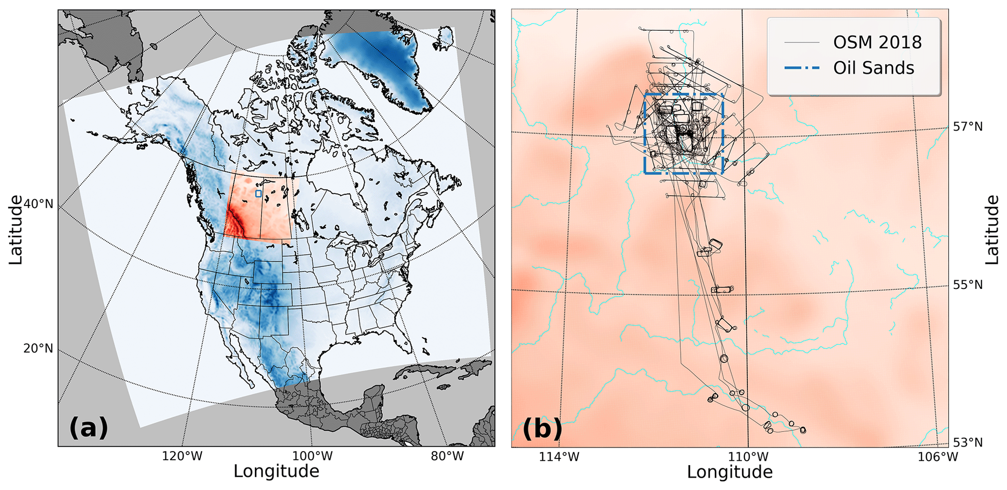
Figure 1 (a) The GEM-MACH model nesting configuration with a parent domain at a 10 km resolution over North America (blue-shaded area) and a nested domain at a 2.5 km resolution (red-shaded area) over Alberta and Saskatchewan provinces. The approximate perimeter of Athabasca oil sands is shown with a blue rectangle. (b) The oil sands region within the 2.5 km domain is depicted with flight tracks (dark lines) from the OSM 2018 aircraft campaign overlaid on the map. The region encompassing the surface mining facilities of the Athabasca oil sands is shown by a dashed blue line. Most of the region's SO₂ emissions occur from large stacks associated with the upgrading of bitumen at surface mining facilities within the dashed-line area.

2.3 Case studies

We considered a simulation period for 2018 over the Canadian oil sands (OS). This period overlaps with the Oil Sands Monitoring (OSM) 2018 aircraft campaign over the oil sands region between April and July of 2018. The aircraft campaign is discussed in Sect. 2.5. For our standalone tests with PRISM (offline PRISM), we used observed stack parameters (e.g. exit temperature, volume flow rate) for the main stacks in three OS facilities (Syncrude, Suncor, and Canadian Natural Resources (CNRL)). We also incorporated meteorological vertical profiles at the locations of these stacks, extracted from retrospective GEM model runs, as input information for PRISM plume height predictions. These predictions were then compared to aircraft-observed heights for SO₂ plumes emitted from the OS stacks of interest. Further, we performed high-resolution (2.5 km grid spacing) air quality simulations with the GEM-MACH model, focusing on the Athabasca oil sands region. Our new plume rise algorithm PRISM was implemented with the high-resolution GEM-MACH simulations (GM-PRISM) for a 6-month model run (February to July 2018 inclusive) and was compared to simulations carried out with the previous scheme (GM-orig) (the latter lacking full stratified calculations of plume buoyancy and water latent heat release/uptake; Akingunola et al., 2018). Model output data from the simulation period were compared to data from the Wood Buffalo Environmental Association (WBEA) surface monitoring network for the region and to aircraft observations from the OSM 2018 campaign. In our analysis, we focused on plumes emitted from the three main (largest) SO₂-emitting facilities: Syncrude, Suncor, and CNRL. We compared model-generated SO₂ fields to aircraft SO₂ measurements from 11 box flights around the 3 facilities of interest. The aircraft data allow us to directly compare model and observed SO₂ plume heights and thus provide a direct estimate of plume rise accuracy (the surface monitoring network data, the analysis of which follows the plume height evaluation, allow us to estimate the effect of the changes on surface SO₂ concentration predictions). Four of these flights were conducted in April and May of 2018 (2 flights each month), and the rest (7 flights) were conducted in June of 2018. Hence, while April in this region is snow-covered and represents emissions under winter conditions, the majority of available aircraft data were for the summertime. Aircraft-measured and interpolated wind and SO₂ data were used to determine plume origins (emission sources). We note that the box flights were designed with the intent of sampling plumes from specific facilities; combined with the aircraft wind speed and direction data, the emissions associated with the source within an enclosing box flight can be distinguished from other sources in the region (see Sect. 2.5). Flight planning included wind and air quality forecasts that allowed box flights to avoid conditions under which a plume from one facility impacted the air above another facility and to avoid conditions that might lead to inaccurate retrievals of emissions levels based on aircraft data (see Fathi et al., 2021). SO₂ data recorded during the segments of the flights corresponding to model output data were analyzed to determine plume centre heights (height of the maximum observed concentrations). The observed heights were compared to model-predicted plume heights using the two plume rise algorithms, GM-orig and GM-PRISM. The results of these evaluations and comparisons are presented in Sect. 3.

2.4 Input emission rates and source parameters

Water vapour (H₂O) and carbon dioxide (CO₂) emission rates from sources within the OS facilities are neither reported in emission inventories such as National Pollutant Release Inventory (NPRI: ECCC, 2023) nor form a part of the continuous emission monitoring system (CEMS). However, their emissions are correlated with fuel combustion as part of OS production/activities: CO₂ and NO_x emissions are related to synthetic crude oil production at the OS (Liggio et al., 2019). For this work, NO_x emission rates, which are reported in the NPRI and CEMS datasets, are used as a proxy for estimating CO₂ emission rates and the corresponding water emission rates determined from combustion reaction stoichiometry. The stoichiometry of the relative amounts of water to CO₂ emitted for a given fuel thus provides an estimate of the water emitted due to combustion. Wren et al. (2023) calculated the average ratios of CO₂ to NO_x emission rates from OSM 2018 aircraft campaign data for individual OS facilities and source types (e.g. stack, area). For this work, the CO₂ : NO_x ratios estimated by Wren et al. (2023) for the stack sources were used in turn to estimate CO₂ emission rates from NO_x reported in NPRI and CEMS. CO₂ and H₂O are primarily generated from combustion of natural gas, with methane (CH₄) as its main component, in OS production operations:

$$\begin{array}{}\text{(R1)}& {\mathrm{CH}}_{\mathrm{4}}+\mathrm{2}{\mathrm{O}}_{\mathrm{2}}⟶{\mathrm{CO}}_{\mathrm{2}}+\mathrm{2}{\mathrm{H}}_{\mathrm{2}}\mathrm{O}.\end{array}$$

Therefore, for every mole of CO₂, 2 moles of H₂O is emitted due to combustion. Accordingly, a stoichiometric ratio of 1 : 2 of CO₂ to H₂O can be used to estimate H₂O emissions levels, as was done for this work. H₂O emissions were then calculated from NPRI- and/or CEMS-reported NO_x emission rates based on source-specific CO₂ to NO_x ratios. For the period corresponding to the aircraft study, the continuous emissions monitoring system (CEMS) hourly data were available for SO₂ and NO_x for only two of the OS Suncor stack sources and for SO₂ for the other facilities/stacks. Canadian emissions reporting requirements for NPRI reporting for large stacks are for annual totals. Therefore, the hourly NO_x and consequently hourly H₂O for the rest of the facilities were estimated from NPRI annual emissions data. CEMS hourly data for stack parameters (e.g. exit temperature, flow rate) and SO₂ emission rates were available for April to July 2018, partially overlapping with the period of our 6-month run simulations from February to July 2018, and were used in the simulations for the same period. We note that the estimation of stack water emissions is a required input for our algorithm – the methodology demonstrated here is easily expandable to other combustion stack sources. Knowledge of the fuel type is required, with different fuels having different amounts of water produced per carbon atom combusted – i.e. Reaction (R1) depends on the fuel used for generating heat for stack emissions. As we will discuss below, the accuracy of the stack emissions and the consequent estimates of water emissions have a key impact on the accuracy of our plume rise algorithm. Note that we used the estimates of combustion-generated water as described above in our simulations (both standalone and GEM-MACH simulations with PRISM) for the specific stack sources for which the following information was available: (a) reported NO_x emission rates (CEMS or NPRI) and (b) facility-specific estimates (aircraft-based) of CO₂ to NO_x emission ratios. Such source emission information was not available for the majority of the stack sources within our large-scale GEM-MACH modelling domain (10 km resolution domain over North America, 2.5 km resolution domain over Alberta and Saskatchewan). Nevertheless, in our GEM-MACH simulations with PRISM (GM-PRISM), the plume rise from major point sources, including those without combustion-generated water data, was also impacted by the moist thermodynamics of the entrained water from ambient air.

2.5 Aircraft campaign and WBEA surface monitoring network

During the OSM 2018 campaign (April to July), aircraft-based measurements of environmental variables (meteorology, pollutant concentrations) were conducted over the Canadian oil sands (OS) (ECCC, 2018). Figure 1b shows the flight tracks taken by the aircraft during the OSM 2018 campaign over the OS region. The aircraft conducted several flights during different days and times from April to July 2018, including single screen flights tens of kilometres downwind of OS facilities and box flights around the facilities at near range. The designation box flight refers to a flight pattern during which the aircraft would fly along closed loops around a specific emitting facility at several consecutive altitudes while making measurements of environmental variables. The box flights were specifically designed to capture emissions from individual facilities. Aircraft-measured data during box flights were converted into source emission rates through flux estimations and mass-balance calculations, utilizing the Top-down Emission Rate Retrieval Algorithm (TERRA) algorithm described in Gordon et al. (2015). For further discussion on the application of TERRA and the uncertainties in emission rate retrievals based on aircraft measurements, see Fathi et al. (2021). This was done for several emitted species such as SO₂, NO_x, and CO₂. As discussed in Sect. 2.4, aircraft-based estimates, emission inventory data, and continuous emissions monitoring system (CEMS) data for NO_x were used to derive the NO_x to CO₂ emission rate ratio, which in turn was used to estimate the water emissions rate.

Here, we also used aircraft measurements of SO₂ concentrations downwind of several oil sands facilities (CNRL, Syncrude, and Suncor) to determine observed plume heights and evaluate our model-predicted plume rise (using both GM-orig and GM-PRISM) vs. these observations. For our analysis, we considered aircraft data from box flights where measurements were made just a few kilometres downwind or upwind of emission sources. This was done to avoid flights that included a large long-range transport path/time of emitted pollutant to the point of measurement so that the observed plumes would be a better representation of emission and plume rise conditions at the stack locations. We focused on SO₂ as the emitted pollutant, since it is a primary emitted pollutant (i.e. not generally generated due to photo-chemical reactions in the atmosphere) and due to the availability of CEMS-based direct observations of SO₂ within emitting stacks. SO₂ in oil sands (OS) regions is mainly emitted from large high-temperature stack sources (over 90 % of the emitted SO₂ in the region originates in the large stacks, unlike NO₂, only about 40 % of which is emitted from large stacks; Zhang et al., 2018), with low background levels from other sources, making SO₂ a good indicator of buoyant plumes and suitable for our study of plume rise parameterization.

Further, we evaluated model performance in terms of surface concentrations of SO₂ vs. air quality observations from 21 WBEA (Wood Buffalo Environmental Association) continuous surface motoring stations in Alberta. Here, we focus on SO₂ as a primary emitted pollutant. Given that SO₂ is mainly emitted from large smokestacks in the OS region (over 90 %; Zhang et al., 2018), this makes it more relevant for our purposes: evaluating the plume rise parameterization for buoyant sources. We analyzed the hourly WBEA data from February to July 2018 vs. GEM-MACH-model-generated fields (from both GM-orig and GM-PRISM) for the same period.

3 Results and discussion

3.1 Model sensitivity to plume rise parameterization: standalone PRISM simulations

We investigated the impact of within-plume combustion-generated water on the neutral buoyancy height of the effluents from high-temperature stacks using PRISM (standalone). Figure 2 shows the dependence of plume final height on stack temperature and the amount of water released within the plume parcel for an idealized case with a dry adiabatic lapse rate. The range of stack temperatures and water emissions is taken from the corresponding reported parameters for the stacks of interest for three oil sands (OS) facilities: CNRL, Suncor, and Syncrude. Note that initial in-plume water vapour was limited to values less than or equal to the saturation level dictated by the saturation vapour pressure for each given stack exit gas temperature (note the cutaway in the surface plot in Fig. 2 and that the high temperatures allow for much higher water content than might be found at ambient temperature conditions). The dependence on stack exit temperature is evident from the results shown in Fig. 2 – i.e. higher stack temperature corresponds to higher plume parcel (initial) buoyancy and the resulting increase in the final height reached by the plume parcel (neutral buoyancy height). The other interesting observation is the stronger dependence on the amount of water vapour emitted. Our results show the significant impact of latent heat exchange due to phase changes in within-plume water on plume rise (Fig. 2). The net release of latent heat as the water vapour condenses within the rising plume modulates plume parcel buoyancy significantly, resulting in up to 500 m of additional rise for the case shown in Fig. 2; compare the plume height values (vertical axis, Fig. 2a) for zero water emissions to those at maximum water emissions. The dependence trends (the cross-sectional trends in Fig. 2) reveal that plume neutral buoyancy height is impacted by moist thermodynamics more significantly than by parcel initial temperature.

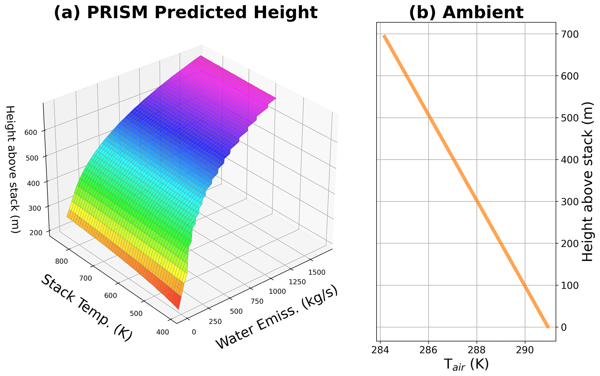
Figure 2 (a) The standalone PRISM-predicted final plume rise for an idealized case as a function of stack temperature and emitted water. (b) The idealized ambient profile for air temperature (with the dry adiabatic lapse rate) is shown as a function of height. Plume neutral buoyancy height shows stronger dependence on initial in-plume water vapour than stack temperature, resulting in up to 500 m of additional rise for the range shown.

We also investigate the impact of moist thermodynamics on plume rise for realistic cases with more complex atmospheric vertical structures. Using the GEM numerical weather model (see Table A1) at a high resolution (2.5 km grid spacing), we generated meteorological fields (wind, ambient air density, temperature, and vapour and liquid water mixing ratios) for the 2018 aircraft campaign over the oil sands region. We used the model-generated meteorological fields (vertical profiles) corresponding to the period of 11 box flights around 3 OS facilities (Suncor, CNRL, Syncrude) as input for PRISM. Further, we used stack parameters (temperature, volume flow rate, water emission rate) for high-temperature stacks within these three facilities to model plume rise using PRISM (offline – i.e. not embedded within the GEM-MACH 3D model). Figure 3 shows the results for the case on 6 June 2018 for the Syncrude main stack. Plume parcel temperature (T), density (ρ), water vapour mixing ratio (q_v), condensed water mixing ratio (q_c), and parcel rise speed are compared to environmental parameters as a function of height in Fig. 3. The PRISM-predicted parcel state variables are shown for four different rise cases: vertical and bent-over rise with and without in-plume water. The without in-plume water (dry) rise cases, illustrated by dashed curves, show how parcel temperature drops (and density increases) as the rising parcel mixes with the ambient air (through entrainment) until it reaches the neutral buoyancy height (height at which the parcel density approaches ambient air density). Note that for the bent-over plume rise, the parcel volume flux is a function of the horizontal wind speed U (cross-wind is shown by a blue curve in Fig. 3e) according to Eq. (2). Consequently, even in the presence of mild cross-winds (2 to 5 m s⁻¹), expansion (due to entrainment) and the buoyancy reduction rate are higher for the bent-over rise than the vertical rise, and therefore, the parcel reaches neutral buoyancy at lower altitudes (Fig. 3). PRISM performs both (vertical and bent-over) calculations for each plume rise case and following Briggs (1984) chooses the final rise calculated by the one resulting in higher buoyancy reduction as a function of height. The impact of latent heat exchange can be seen for the moist plume rise cases, shown by solid curves in Fig. 3. The condensation of in-plume water (and the resulting latent heat release) prolongs parcel buoyancy for both rise types (vertical and bent-over), resulting in a higher final rise compared to the dry cases. Note the difference in condensed water (q_c) vertical profiles for the bent-over (green) and vertical (orange) rise types in Fig. 3d. Water condenses faster (and at lower altitudes) for the bent-over rise, but it is short-lived compared to the vertical rise. The corresponding impact on parcel temperature (T) and density (ρ) can also be seen in Fig. 3a, b: parcel temperature drops (and parcel density increases) with height at a lower rate for the period of latent heat release (compared to rise with no latent heat exchange), and as a result, the parcel state variables approach ambient values at much higher altitudes. Note that the height at which parcel plume density approaches ambient air density, within an acceptable level of accuracy (defined as a convergence criterion of the difference between parcel and ambient air density relative to the ambient air density below a threshold), is taken as the plume neutral buoyancy height. Under most convective conditions (and in the absence of strong inversions), parcel density tends to approach ambient air density asymptotically (see Fig. 3b).

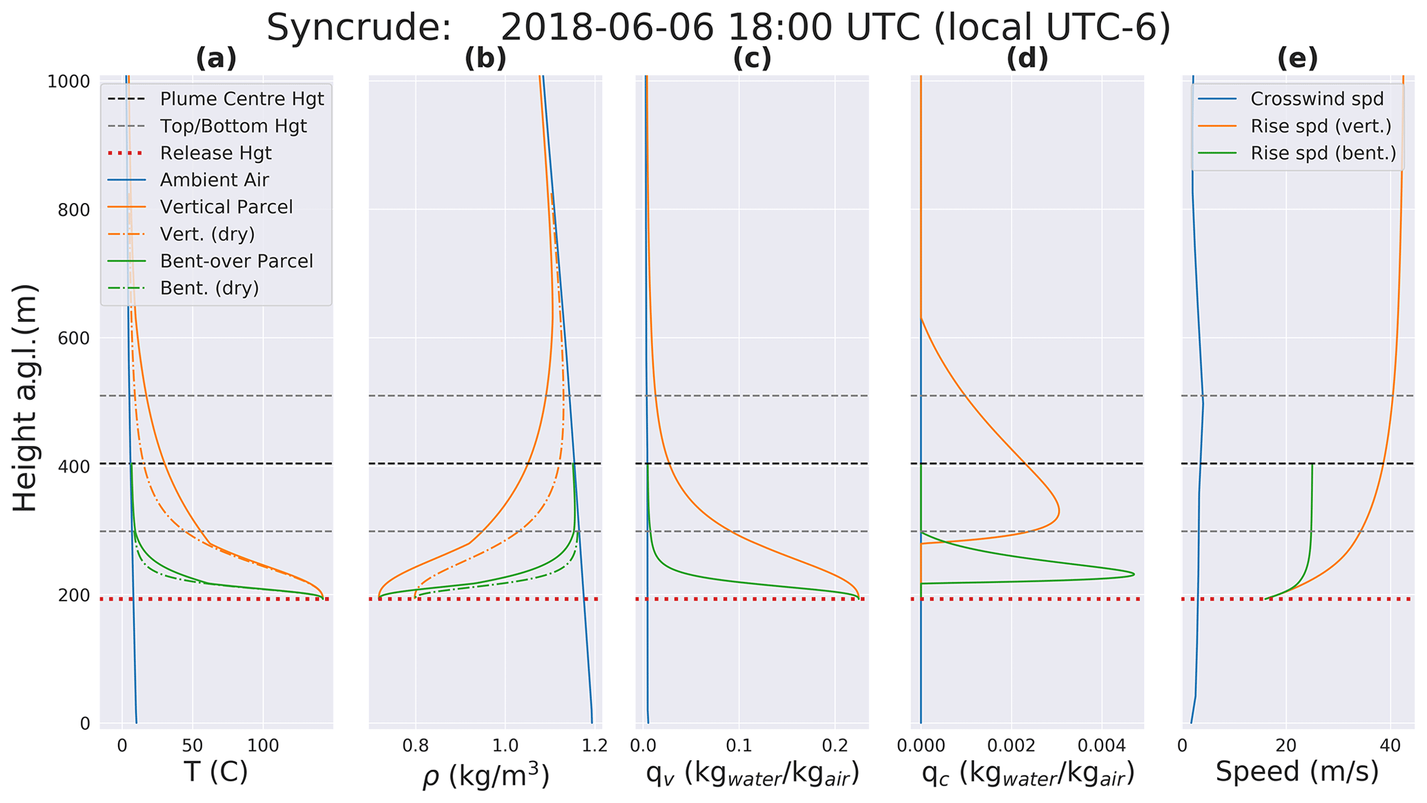
Figure 3 The standalone PRISM-predicted parameters for a rising plume parcel are compared to ambient conditions for four different cases, vertical and bent-over rise (moist and dry), for the main stack at the OS Syncrude facility on 6 June 2018 at 18:00 UTC. Parcel (a) temperature, (b) density, (c) water vapour mixing ratio, (d) condensed water mixing ratio, and (e) rise speed and horizontal wind speed U (crosswind) are shown.

In our standalone tests with PRISM, we have noticed the asymptotic offset between parcel air density and the ambient air density, which depends on the vertical resolution at which buoyancy reduction calculations are performed, falls between 0.1 % and 0.5 % of ambient air density. That is to say, when parcel density starts to asymptotically approach the ambient air density, as a result of the finite resolution of the calculations and the slight excess humidity within the plume parcel, plume density remains offset from the ambient density within a fraction of a percent of the ambient air density at those heights, although it follows the same lapse rate as the ambient air. Our criteria for convergence is thus based on the observed numerical behaviour of the rising parcel. We believe that the physical reason for the observed situation where the parcel comes to rest without asymptotic rise may reflect detrainment of parcel water to the ambient atmosphere. Future work will focus on evaluating the detrainment impact. PRISM can be configured with different density convergence criteria (ρ_conv) in terms of the percentage difference between parcel and ambient air density: ${\mathit{\rho }}_{\mathrm{conv}}=\left|\right(\mathit{\rho }-{\mathit{\rho }}_{\mathrm{air}}\left)\right|/{\mathit{\rho }}_{\mathrm{air}}\times \mathrm{100}$. At the height where the difference between parcel density and ambient air density falls within ρ_conv, the parcel is assumed to be neutrally buoyant, and the rise terminates. We performed tests with ρ_conv ranging between 0.1 % to 0.5 % and found ρ_conv=0.3 % (by comparing plume rise estimates to aircraft-observed plume heights) to be the optimal convergence criterion for the majority of the cases we considered. We note that the choice of ρ_conv depends on the numerical accuracy of the calculations and the vertical resolution at which the plume buoyancy reduction is calculated. The results shown in Fig. 3 are from calculations at a 1 m resolution. Our tests with different resolutions up to a 10 m resolution have shown optimal performance with ρ_conv between 0.1 % and 0.3 %. We also note that the plume rise algorithm is sensitive to input information such as stack exit temperature, and depending on the confidence level of input parameters, the convergence criteria can be either strict or relaxed.

3.2 Model sensitivity to plume rise parameterization: GEM-MACH simulations

We performed two sets of retroactive simulations with the GEM-MACH model, with the original plume rise algorithm (GM-orig) and with PRISM embedded within GEM-MACH (GM-PRISM). Model outputs from the two sets of simulations were compared for a 6-month period between February and July 2018. Output data were divided into two groups: the wintertime (including the months of February, March, and April) and summertime (including the months of May, June, and July). This was done in order to investigate model sensitivity to the two different plume rise parameterizations for two general sets of conditions: the cold and more stable atmosphere during the wintertime and the warmer and less stable atmosphere during the summertime. The separation of the simulations into the two seasons also allows us to examine the effect of emissions data accuracy on plume rise calculations: we note that the CEMS source parameter and emissions data were available only for April to July 2018 (excluding the months of February and March in the wintertime). The average SO₂ surface concentrations for GM-PRISM summertime simulations, with ρ_conv=0.3 %, are shown in Fig. 4a and b for the oil sands region sub-domain and for the entire high-resolution domain, respectively. Figure 4c, d show GM-PRISM normalized mean bias (NMB) in percent relative to GM-orig simulations for surface SO₂. The confidence ratios at the 90 % confidence level (CR90; see Makar et al., 2021) were also calculated between surface concentrations generated by the two simulations and are depicted in Fig. 4e, f. The confidence ratio values ≥1 are indicative of a statistically significant difference between the GM-PRISM and GM-orig simulations at the specified confidence level (here 90 %). The highest values of CR (e.g. 2 and above) are located close to sources of SO₂, such as the oil sands sources, as well as other sources located to the south and west of the oil sands region (Fig. 4e, f). That is, the impact of the revised parameterization is the strongest close to the sources. We note that due to the lack of sufficient information (e.g. source-specific CO₂ to NO_x emission rate ratios) for reliably estimating the amount of combustion-generated water mass for the hundreds of emission sources (none OS) within the large-scale modelling domain, the emissions of combustion water were only available for a number of OS facilities (e.g. aircraft-based facility-specific NO_x to CO₂ emission ratios). For those major point sources without water emissions, the differences between the algorithms are due to the entrainment of ambient water into dry combustion plumes and the stratified calculation of plume buoyancy in PRISM. For major OS point sources with water emissions, the differences are further influenced by the moist thermodynamics of the combustion-generated water. Nevertheless, differences can be seen for all large stack sources of SO₂ within the domain, showing the impact of the revised algorithm on SO₂ even in the event that water emissions are not available; entrained water interacts with the emitted parcels and may have a significant impact on plume rise and SO₂ dispersion, with differences between the two simulations exceeding the 90 % confidence level (CR90 > 1) for about 7 % of the entire modelling domain (Fig. 4). The impact of combustion-generated water on plume rise for OS stacks is apparent from Fig. 4e, with CR90 > 1 for more than 20 % of the model domain corresponding to the oil sands region (the region within the dashed box in Fig. 4e). CR90 ≥ 1 values near large stack sources clearly demonstrate that the plume rise algorithms predicted different plume heights at source locations, resulting in different vertical distributions of the SO₂ plumes and significant differences at the surface. These differences become less pronounced farther away from the emission sources, although some regions of significant differences (also significant at lower confidence levels, e.g. CR80 ≥ 1, CR85 ≥ 1) can occur far downwind of the sources (e.g. northern Saskatchewan; the CR90 ≥ 0.4 region in the middle-right of Fig. 4f). The downwind differences demonstrate the change in the direction and the range of the transport of the emitted SO₂ mass. This is a direct result of the difference in rise parameterization due to the plumes rising to different altitude levels with dissimilar flow regimes (e.g. wind speed and direction, strength of turbulence). Similarly for the wintertime, the differences between GM-PRISM- and GM-orig-simulated surface SO₂ were pronounced near emissions sources but to a greater spatial extent, with CR90 ≥ 1 for 50 % of the model domain corresponding to the oil sands region (see Fig. S1 in the Supplement for wintertime comparisons). For the wintertime, CR90 ≥ 1 values correspond to about 10 % of the entire modelling domain. The differences between summertime and wintertime results are partially attributable to drier and more stable conditions in the colder months compared to more humid and convective conditions in the warmer months. Generally, the new parameterization predicted lower plume heights and weaker vertical mixing of the emitted SO₂ mass compared to summertime. Also note that combustion-generated water emissions information, CEMS emissions data, and stack parameter data were not available for the majority of the wintertime simulations.

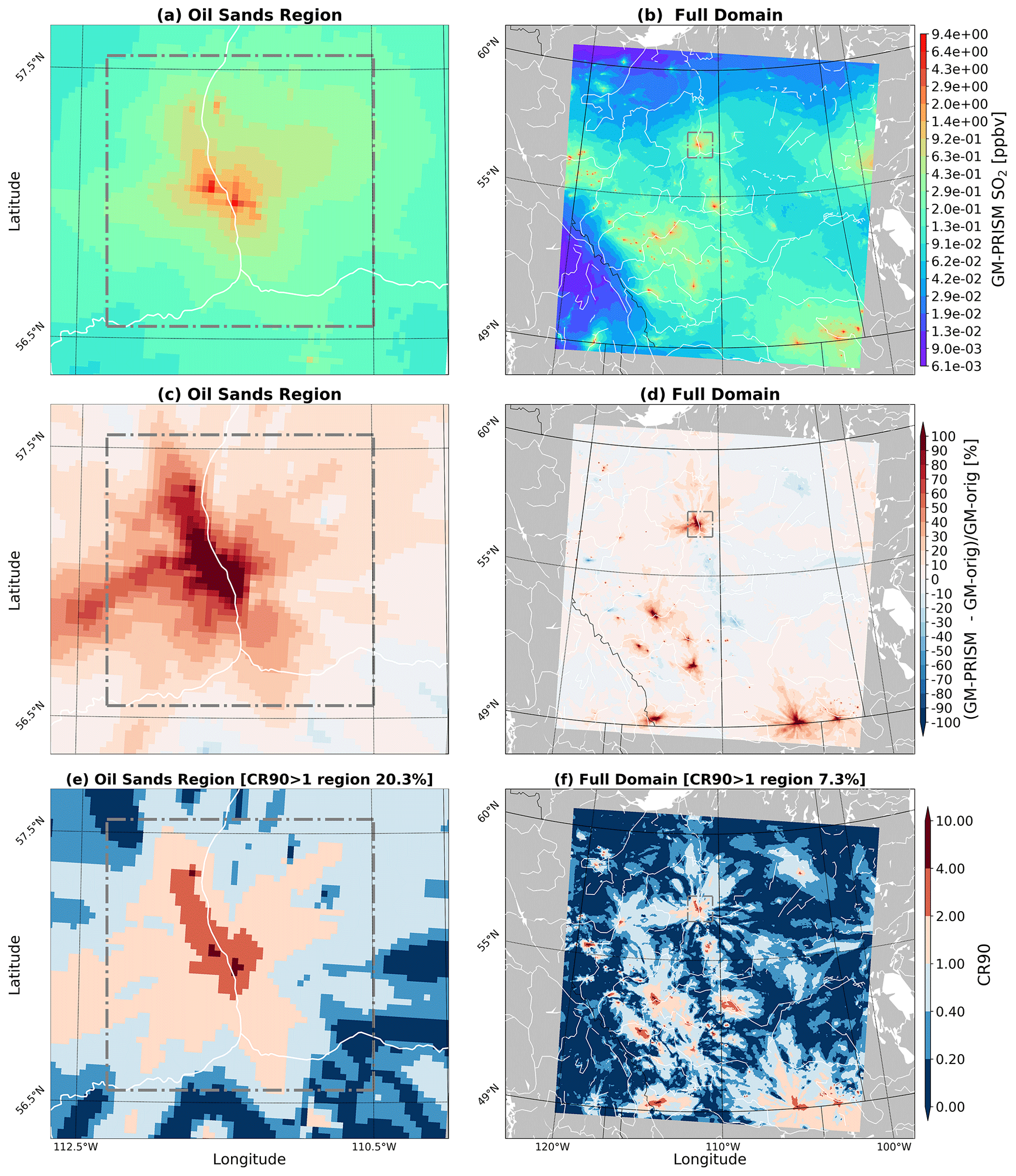
Figure 4 Average surface SO₂ concentrations for the summertime period (May, June, and July 2018) generated by GM-PRISM simulations with ρ_conv=0.3 %, shown for (a) the oil sands region and (b) the entire domain. (c, d) Normalized mean bias (NMB) in % relative to GM-orig simulations for the same period. (e, f) Confidence ratio at a 90 % confidence level (CR90).

The GM-orig algorithm parameterizes the plume rise based on flux reduction calculations as a function of atmospheric stability (Akingunola et al., 2018), whereas the GM-PRISM algorithm performs direct flux reduction calculations at each vertical level while accounting for heating/cooling due to phase changes in water. Consequently, the GM-PRISM algorithm is more sensitive to input stack parameters and in-plume water mass data. We note that hourly CEMS data (direct measurements) of source parameters (e.g. effluent exit temperature and volume flow rate) were only available for the period between April and July 2018 (April plus summertime) as input for model simulations. The input stack parameters for the months of February and March ($\mathrm{2}/\mathrm{3}$ of wintertime) were based on the reported parameters in the Canadian National Pollutant Release Inventory (NPRI). The reported stack parameters are the “optimal” values for a given stack but may not correspond to hour-to-hour variations. The winter stack parameter estimates are largely indirect (based on other factors such as design parameters of the stack) at low temporal resolutions (i.e. based on annual total emissions data; AER, 2022). This adds further uncertainty to wintertime evaluations of GM-PRISM simulations.

3.3 Plume rise prediction evaluation vs. aircraft-observed SO₂ plumes

Model plume height predictions by GM-orig and GM-PRISM corresponding to 11 box flights during the OSM 2018 campaign were evaluated vs. aircraft observations for SO₂ plumes. Aircraft measurements of wind and concentration fields at several altitude levels around the major SO₂-emitting OS facilities, Syncrude, Suncor, and CNRL, were analyzed to determine the source stack of each observed plume. Note that ambient atmospheric meteorological variables were extracted from the GEM-MACH simulations and used as meteorological inputs for the algorithm. Plume centres for each flight case were identified and their altitudes estimated from the interpolated concentration data (see Fig. S2). These observed plume heights were then compared to plume height predictions by GM-orig and GM-PRISM (ρ_conv=0.3 %) simulations for the corresponding times and locations. Figure 5 shows the comparisons between hourly model-predicted plume heights at the stack location and aircraft-measured vertical profiles of SO₂ concentrations corresponding the same model hour. The flight strategy for these box flights was to encircle the facility, starting the aircraft flights around the facility close to the surface and increasing in altitude as the aircraft flew around the facility: a box-shaped spiral flight pattern, gradually increasing in height (see Fig. S2). High concentrations of SO₂ on a given pass around the facility were taken as a tentative plume height on each pass as the aircraft rose in altitude. However, the highest concentration encountered during the entire set of passes was used to represent the plume height, with lower concentrations encountered during the course of the flight representing either the edges of a rising plume or lower-concentration plumes due to other sources within the facility and region (Fig. S2). In some cases, during the course of a flight, the apparent equilibrium plume height (determined from the highest concentration encountered during a given pass around the facility) changed, possibly reflecting an ongoing change in plume height due to changing atmospheric conditions (Fathi et al., 2021). That is, the top of the plume was able to be distinguished close to the surface and then again at a higher level on a subsequent higher-altitude pass of the aircraft, suggesting either a rising plume during the course of the study or multiple layers of SO₂ within the box domain. The final estimation of the plume height in these cases was the location of the highest concentration encountered during the course of the flight. In Fig. 5, we show the normalized concentration of SO₂ measured at each hour by the aircraft, indicating the height of the observed plume using the maximum concentration at each time. For flights 4, 7, 9, 10, 17, and 21, the plume height increased during the course of the flight. In flights 6, 8, 11, 19, and 20, the plume height remained stable. In some of the cases where the plume height increased, the estimate of the observed height at the first hour (the lowest-elevation passes around the facility) is highly uncertain since the flight had yet to reach the height at which the entire vertical extent of the plume was sampled. Flights 4, 7, 9, 10, 17, and 21 are examples where the aircraft sampling during the initial hour may not have reached sufficient heights to sample the entire plume. The maximum concentration recorded by the aircraft during each hour was then compared to hour-by-hour model-predicted plume heights. Model values for the plume height at each hour are shown in symbols in Fig. 5 (grey lines and circles – GM-orig; orange lines and squares – GM-PRISM), and the upper and lower extent of the simulated plume via Eq. (14) is shown as a grey (GM-orig) or orange (GM-PRISM) shaded region. Note that most of these flights were conducted during local noon and afternoon hours under convective conditions (see Fig. S3 for model-predicted vs. aircraft-observed temperature profiles). Therefore, it is reasonable to assume a temporal variation in the vertical mixing of the observed plumes. Such temporal trends were captured by both GM-orig and GM-PRISM simulations, as can be seen in Fig. 5.

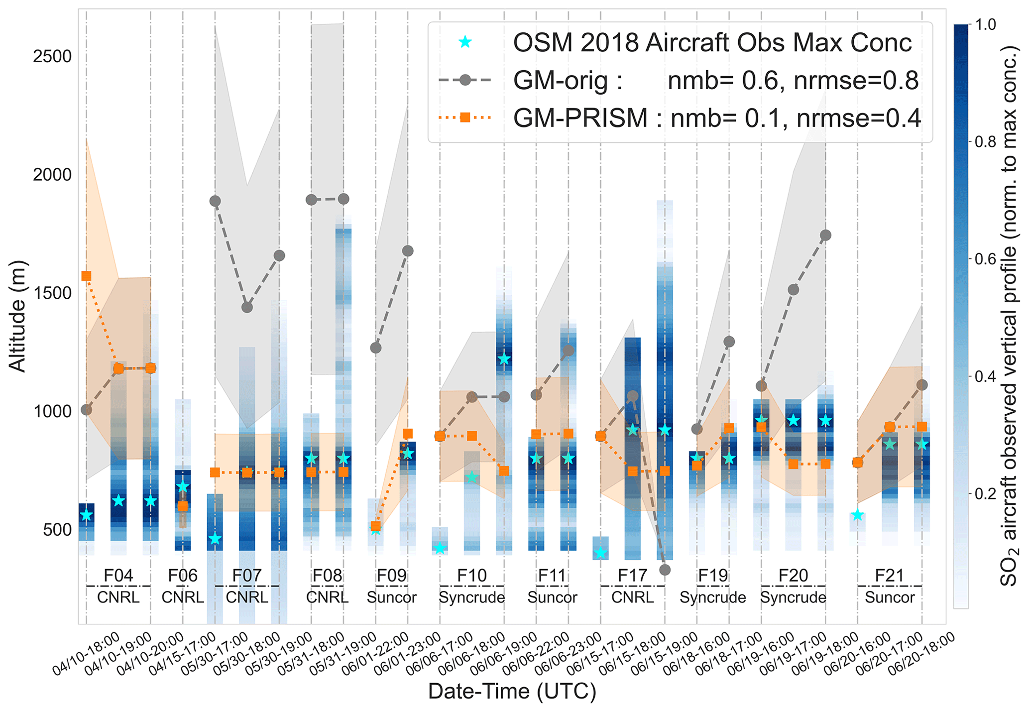
Figure 5 Predictions of plume height in GM-orig and GM-PRISM simulations compared to OSM 2018 aircraft observations for the 11 case studies. For each hour of the flight, aircraft-observed vertical profiles of concentration are shown as density maps (white to blue) up to the height visited by the aircraft by that hour. Concentrations are shown as shaded blue regions, which have been normalized to the maximum concentration encountered during the flight. Aircraft-observed SO₂ plume maximum concentration heights are marked with cyan stars and are taken here to represent the observed plume heights. Plume maximum concentration height predictions by GM-orig (grey circles) and GM-PRISM (orange squares) are compared with the aircraft-observed heights (flight median). Results are shown as the normalized mean bias (NMB) and normalized root-mean-squared error (NRMSE).

GM-PRISM showed a significant improvement relative to GM-orig in 8 of the 11 flights (flights 7, 8, 9, 11, 17, 19, 20, and 21). For these cases, GM-orig was shown to overestimate the plume height by up to a kilometre (e.g. flight 8), while the distance between measured and modelled plume heights is greatly reduced with GM-PRISM simulations. For two flights (flights 6 and 10), the two algorithms produced similar plume heights, and for one flight (flight 4), both approaches resulted in a considerable overestimate of plume height (possibly due to a positive bias in model temperatures that is discussed later). Figure 5 compares GM-orig- and GM-PRISM-simulated plume maximum concentration heights (GM-orig – grey line; GM-PRISM – orange line) to the median of maximum concentration heights observed during flight/sampling time. The tendency of GM-orig to overestimate plume height can be seen clearly, as can the general overall improvement in plume height with GM-PRISM. The summary values for the normalized mean bias (NMB) and normalized root-mean-square error (NRMSE) in the plume heights are shown in Fig. 5; the use of GM-PRISM has substantially reduced the magnitudes of both error metrics, with the NMB decreasing from 60 % to 10 % and the NRMSE being halved. The new parameterization thus provides a clear improvement in the plume height estimate compared to the previous algorithm, indicating that the stratified calculation of plume buoyancy and latent heat exchange associated with in-plume water has a significant impact on plume rise.

We note that GM-PRISM overpredictions for flight 4 (wintertime) are partially due to a positive bias of a few degrees Celsius in model temperatures relative to aircraft measurements (see Fig. S3). When this temperature bias is corrected for, GM-PRISM plume height predictions can be further improved. This demonstrates the sensitivity of the new parameterization (GM-PRISM) to the input ambient temperature profiles. Over/underpredictions, similar to the case of flight 4, can potentially be related to model temperature biases, although insufficiently precise stack parameter data may also play a role, as discussed above. Using aircraft-observed temperature (vertical) profiles as input into standalone PRISM simulations (not embedded within the GEM-MACH model), we were able to confirm this effect for flight 4 (a reduction in error parameters by about 10 % in the NMB). We note that for the current work, we had wintertime aircraft data from only two flights (4 and 6), while a larger observational dataset is needed for a more comprehensive investigation of such effects. Note that the ambient air data required as input for the PRISM algorithm include horizontal wind speed, air density, air pressure, and the water content (vapour, liquid, ice) mixing ratio in addition to temperature profiles. For the flight 4 example, only temperature profiles were replaced with aircraft-observed temperatures, and the rest of the ambient air input data were from the GEM model output. Note that the combustion-generated water data, derived from the CEMS and NPRI emissions data of NO_x (Sect. 2.4), were included in GEM-PRISM simulations. The results shown in Fig. 5 show the impact of the new parameterization, including the stratified calculations of buoyancy and moist thermodynamic effects of both entrained and emitted water.

3.4 Impact of plume rise parameterization on GEM-MACH's surface SO₂ concentration performance

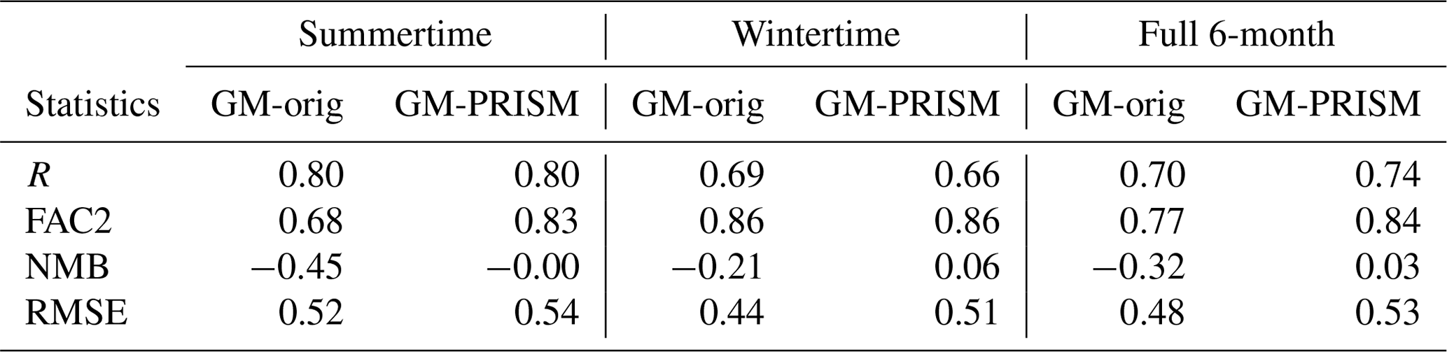
Evaluations vs. the WBEA continuous monitoring network confirm the results vs. aircraft-observed SO₂ plumes and show the substantial impact of moist-plume rise on downwind SO₂ concentrations, with GM-PRISM improving the prediction of surface SO₂ concentration relative to GM-orig predictions for the study period. Figure 6 shows the evaluation of monthly average surface SO₂ produced by the model when making use of the two plume rise calculations vs. observations at WBEA continuous monitoring stations in the oil sands region. Comparisons are shown for the summertime (May, June, and July, when CEMS data were available) in Fig. 6a, b and the wintertime (February, March, and April, when CEMS data were mostly unavailable) in Fig. 6c, d. Figure 6b and d show SO₂ mean biases by GM-orig and GM-PRISM (with ρ_conv=0.3 %) at the locations of WBEA stations over the OS region. Evaluation results show biases of various degrees by GM-orig and GM-PRISM simulations. The GM-PRISM method improved surface SO₂ predictions relative to GM-orig for the summertime, with the fraction of predictions within a factor of 2 of observations (FAC2) increased from 0.68 to 0.83 and the normalized mean bias (NMB) reduced significantly, from −0.45 to −0.00, as summarized in Table 1. GM-PRISM also improved the wintertime surface SO₂ predictions relative to GM-orig in terms of mean bias, reducing NMB from −0.21 to 0.06 (Table 1). We note that wintertime results are less conclusive due to the absence of CEMS emissions and stack parameter data as model input for most of the winter period. We note that due to the strong spatial heterogeneity of concentration fields (SO₂), evaluations vs. observations at individual WBEA stations resulted in diverse statistics. This in turn demonstrates the impact of different plume rise parameterizations on modelling the dispersion (transport direction and range) of pollutants. We also note that different choices for the plume parcel convergence criteria ρ_conv result in different levels of performance by the PRISM algorithm. Our tests with a previous version of the emissions and stack parameter input data using ρ_conv values of 0.1 %, 0.3 %, and 0.5 % resulted in summertime NMB scores of −0.27, −0.06, and 0.17, respectively (see Tables S1, S2, and S3 in the Supplement). With ρ_conv=0.5 % resulting in an overestimation and ρ_conv=0.1 % resulting in an underestimation of surface SO₂ concentrations for the full 6-month simulation (including both CEMS and non-CEMS periods), ρ_conv=0.3 % was found to be the optimal convergence criterion for our modelling study. GM-PRISM simulations with ρ_conv=0.3 % resulted in a relatively small bias of 3 % (compared to −32 % by GM-orig) over the entire 6-month simulation period, as shown in Table 1.

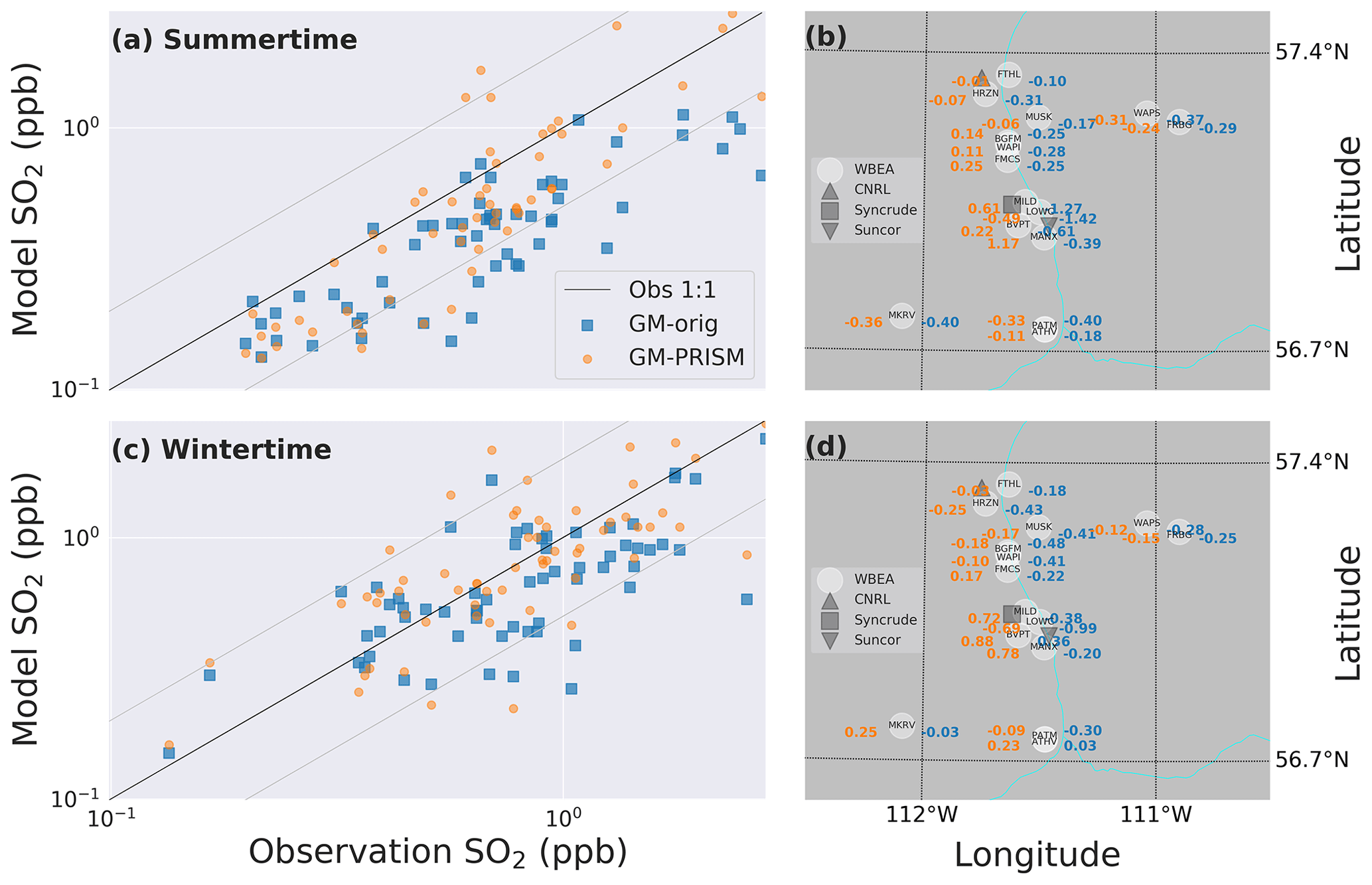
Figure 6 Evaluations vs. WBEA monthly average surface SO₂ observations. Comparisons for (a, b) summertime and (c, d) wintertime are shown. Panels (b) and (d) show model mean bias in ppb (GM-orig in blue, GM-PRISM in orange) vs. observations at WBEA stations on the map of OS region for summer and winter, respectively. Also shown in (b) and (d) are the locations of the WBEA continuous monitoring stations (white circles) and the OS facilities Syncrude (square), Suncor (downward triangle), and CNRL (upward triangle). WBEA station IDs are noted on the corresponding white circles.

Table 1 Statistical comparison of average monthly SO₂ surface concentrations vs. WBEA continuous monitoring data with GM-orig and GM-PRISM (with ρ_conv=0.3 %) simulations for the period from February to July 2018. R is the correlation coefficient, FAC2 is the fraction of predictions within a factor of 2 of observations, NMB is the normalized mean bias, and RMSE is the root-mean-squared error.

Several factors may contribute to model bias (with both GM-orig and GM-PRISM). These can potentially be related to the performance of the meteorological model in simulating mixing conditions for the same locations and time periods, which would require further investigation, including comparisons to observed surface temperatures and vertical temperature profiles. Another possible reason is the coarse resolution of the model, with 2.5 km grid spacing and numerical dilution of mixing ratios, rendering model-generated surface concentrations less representative of near-source observed values. Russell et al. (2019) used GEM-MACH simulations at 2.5 and 1 km resolutions to demonstrate that increased resolution can result in a local increase in concentration, suggesting that model simulations at higher resolutions can potentially improve model performance and reduce the negative bias at the surface. This needs further investigation using simulations at even higher resolutions (e.g. 50 m; Fathi et al., 2023). A key difference between the summer and winter simulation periods is the availability of time-specific stack parameters from hourly CEMS data (stack parameter, emissions) as input for model simulations, which added further uncertainty to wintertime evaluations. For the summertime period, for which CEMS data were used as input for simulations, the PRISM algorithm improved the predictions significantly, in terms of both plume final height and surface concentrations in evaluations vs. observed values. We note the significance of the improved predictions of plume height by the PRISM algorithm under highly convective and complex summertime conditions (where enhanced turbulence plays a greater role in dispersion relative to the more stable conditions of wintertime).

4 Conclusions

In this work, we investigated the behaviour of pollutant plumes emitted from industrial stacks under various atmospheric dispersion conditions in the context of plume rise modelling. As demonstrated in this work, the vertical distribution and downwind dispersion of pollutants emitted from high-temperature anthropogenic sources are controlled by plume parcel buoyancy and water content as well as by ambient atmospheric conditions. We explored the impact of moist thermodynamics on buoyant plume rise from industrial sources through the development of a new plume rise parameterization, PRISM (Plume-Rise-Iterative-Stratified-Moist). This new approach incorporates the thermodynamic effects of latent heat exchange associated with phase transitions of in-plume water in the empirical formulations by Briggs (1984), while performing layered (stratified) calculations of parcel buoyancy for the rising plume. The effluents emitted from high-temperature stacks include significant amounts of combustion-generated water vapour that can condense as the plume rises and cools. The subsequent heating due to the release of latent heat can prolong the buoyancy of the plumes and result in increased rise above the stack top. Conversely, the evaporation of the entrained liquid water within the plume can result in additional cooling of the effluent and limit the rise. We also note that the addition of condensed water within the plume modifies parcel buoyancy and can act as a rise limiting factor through latent heat loss as this condensed water evaporates.

As the water emissions data were not available for the sources of interest (Canadian oil sands) from the emission inventory datasets, we estimated water emissions from the estimated NO_x and CO₂ emissions based on aircraft measurements during an aircraft campaign in 2018 over the Canadian oil sands (ECCC, 2018). For this purpose we used a stoichiometric ratio of 1 : 2 of CO₂ to H₂O, as methane was assumed to be the primary combustion fuel for the emission sources considered. We demonstrated the significant impact of latent heat exchange due to phase changes in within-plume water on plume buoyancy and the final height reached by the pollutant plumes emitted from anthropogenic sources, using standalone (offline) simulations using PRISM with the reported stack source information for several oil sands sources as input data (stack exit temperature, volume flow rate, and estimated water emissions). Our results show that emitted effluents that contain water vapour can rise up to 500 m higher than dry (no water content) combustion plumes with the same initial exit momentum and buoyancy (see Fig. 2). We showed that plume behaviour has a stronger dependence on plume parcel water content than on effluent exit temperature, suggesting that the addition/removal of water mass in both gas and liquid phases can act (and potentially be utilized) as an effective controlling factor for the height reached by anthropogenic pollutant plumes and their downwind dispersion. We also showed that pollutant plumes can behave differently under dry and humid conditions and in the presence of precipitation, by accounting for the thermodynamic impacts of entrained water (vapour and condensed) from the ambient air into the parcel. Emitted and entrained water was found to impact plume buoyancy and final rise height and may boost or limit the buoyant rise of the plumes. For instance, a plume parcel can maintain its water vapour content and positive buoyancy for a longer duration and up to higher altitudes under humid atmospheric conditions than under dry conditions. Conversely, if water mass (rain droplets, ice, snow) is present in the ambient air, as this water is entrained into the warm plume parcel, it can result in heat loss and latent cooling as the water evaporates (and ice melts) and consequently limit the buoyant rise of the plume. We showed that moist thermodynamics has a wide-ranging impact on plume behaviour and surface SO₂ concentrations over a large region and under varying atmospheric conditions (dry and humid, cold and warm, stable and convective). This was accomplished using a series of retrospective model simulations in which Environment and Climate Change Canada's GEM-MACH air quality model was used, coupled with the PRISM moist-plume-rise algorithm (GM-PRISM), for a 6-month period. These modelling results demonstrate the moist thermodynamic impact, with a ±100 % difference in the average SO₂ concentrations near industrial sources (see Figs. 4 and S1).

Through comparisons with aircraft-observed SO₂ plumes during the OSM 2018 airborne campaign, we further demonstrated the impact of moist thermodynamics on plume behaviour and showed that accounting for such effects can significantly improve plume height predictions, on average by up to 50 % in terms of NMB (normalized mean bias). These impacts were demonstrated to provide a more accurate description of plume rise through evaluations of model performance vs. WBEA surface monitoring network data (surface SO₂ concentrations) that showed significant improvements for the summertime (and moderate improvements for the wintertime) simulations in terms of all statistics (e.g. correlation coefficient and bias; see Table 1 and Fig. 6). These improvements in predictive capabilities by utilizing PRISM further reinforce the fact that moist thermodynamics is a key component of the rise of buoyant plumes and influences the long-range transport and surface concentration of emitted pollutants.

For the period between April and July 2018 (inclusive), where hourly (directly measured) CEMS stack parameters and emissions data were available as model input information, the new plume rise algorithm in GM-PRISM simulations outperformed the older parameterization by 50 % in terms of NMB (reduced RMSE by about 50 %) when calculating the plume final (equilibrium) height (Fig. 5). GM-PRISM also improved statistics (e.g. FAC2, NMB; Table 1) for evaluations vs. the WBEA surface monitoring network data (SO₂) for the same period. Evaluations for the wintertime simulations were less conclusive due to the lack of hourly input data (stack parameters, emissions) and direct aircraft observations of the plume heights. The new plume rise algorithm PRISM is highly sensitive to model input information such as stack parameters and source emission rates. The biases in simulated surface concentrations, especially in the wintertime, may be a function of this missing information. Therefore, further investigation for wintertime conditions using high-resolution (temporal) and source-specific input data is desired as these become available.

This study introduces a novel sub-grid parameterization for plume rise, integrating moist thermodynamics into the iterative calculation of neutral buoyancy height for plumes emitted from industrial stacks. Our analysis underscores the significant influence of moist thermodynamics on plume rise and the subsequent downwind dispersion of emitted pollutants, thus advancing our understanding of plume behaviour under different atmospheric dynamics. We also note that the addition of liquid-phase water due to condensation can potentially impact the within-plume aqueous-phase chemistry and plume composition, which will be further investigated in subsequent research.

Appendix A

Côté et al. (1998a, b)Girard et al. (2014)Moran et al. (2010)Makar et al. (2015a, b)Girard et al. (2014)Makar et al. (2015a, b)Abdul-Razzak and Ghan (2002)Gong et al. (2015)Makar et al. (2015a, b)Stockwell and Lurmann (1989)Gong et al. (2002, 2003)Gong et al. (2015)Makar et al. (2018)Makar et al. (2018)Makar et al. (2003)Bermejo and Conde (2002)Sørensen et al. (2013)de Grandpré et al. (2016)Coats (1996)Zhang et al. (2018)Briggs (1984)Briggs (1984)Akingunola et al. (2018)

Table A1 GEM-MACH model configuration details.