Partitioning anthropogenic and natural methane emissions in Finland during 2000–2021 by combining bottom-up and top-down estimates

Accurate national methane (CH₄) emission estimates are essential for tracking progress towards climate goals. This study investigated Finnish CH₄ emissions from 2000–2021 using bottom-up and top-down approaches. We evaluated the ability of a global atmospheric inverse model CarbonTracker Europe – CH₄ to estimate CH₄ emissions within a single country. We focused on how different priors and their uncertainties affect the optimised emissions and showed that the optimised anthropogenic and natural CH₄ emissions were strongly dependent on the prior emissions. However, while the range of CH₄ estimates was large, the optimised emissions were more constrained than the bottom-up estimates. Further analysis showed that the optimisation aligned the trends of anthropogenic and natural CH₄ emissions and improved the modelled seasonal cycles of natural emissions. Comparison of atmospheric CH₄ observations with model results showed no clear preference between anthropogenic inventories (EDGAR v6 and CAMS-REG), but results using the highest natural prior (JSBACH–HIMMELI) agreed best with observations, suggesting that process-based models may underestimate CH₄ emissions from Finnish peatlands or unaccounted sources such as freshwater emissions. Additionally, using an uncertainty estimate based on a process-based model ensemble for natural CH₄ emissions seemed to be advantageous compared to the standard uncertainty definition. The average total posterior emission of the ensemble from one inverse model with different priors was similar to the average of the ensemble including different inverse models but similar priors. Thus, a single inverse model using a range of priors can be used to reliably estimate CH₄ emissions when an ensemble of different models is unavailable.

1 Introduction

Methane (CH₄) is the second most important anthropogenic greenhouse gas (GHG) after carbon dioxide (CO₂). Its atmospheric concentration has nearly tripled since pre-industrial times, primarily due to human activities (Canadell et al., 2023). Since atmospheric CH₄ measurements began in the late 1970s (Rice et al., 2016), the growth rate of atmospheric CH₄ has varied considerably, with periods of rapid growth, as well as a plateau (Nisbet et al., 2023); the growth rate of CH₄ was close to zero from 2000 to 2006, after which the atmospheric CH₄ levels began to rise again (Nisbet et al., 2014; Mikaloff-Fletcher and Schaefer, 2019), reaching remarkably high increases of 15.15 ppb in 2020 and 17.97 ppb in 2021 (Lan et al., 2024). The reasons for this renewed growth and the record-high CH₄ growth rates in 2020 and 2021 are still under discussion (Nisbet et al., 2023), which reflects the large uncertainties in CH₄ emissions. Reducing CH₄ emissions is an effective way to mitigate climate change (Nisbet et al., 2020; Collins et al., 2018), given the short atmospheric lifetime of CH₄ (9.1 years; Canadell et al., 2023) and its high global warming potential (82.5 times higher than CO₂ on a 20-year timescale; Forster et al., 2023). However, in order to assess the success of the CH₄ emission reductions, we need to improve our ability to quantify CH₄ emissions and their changes.

In the Paris Agreement (UNFCCC, 2015), participating countries committed to reporting their GHG emissions and removals coherently and transparently by compiling national greenhouse gas inventories (NGHGIs). The NGHGIs are evaluated jointly every 5 years in the global stocktake (UNFCCC, 2023) which was completed for the first time in 2023. They are based on a bottom-up approach that starts at the sources and estimates how much GHG is emitted by each source. The main objective is to capture trends caused by (direct) anthropogenic activities in order to track the effect of mitigation efforts put into practice, and thus, the NGHGIs report emissions and sinks as annual country totals. In addition to the NGHGIs, which are compiled independently by each country, there are other bottom-up anthropogenic GHG inventories that are compiled for larger regions or even on a global scale. Such inventories relevant to Finland are, for example, the Emissions Database for Global Atmospheric Research (EDGAR; European Commission and Joint Research Centre et al., 2023), the Copernicus Atmosphere Monitoring Service Regional inventory (CAMS-REG; Kuenen et al., 2022) and the Greenhouse gas and Air pollution Interactions and Synergies (GAINS; Höglund-Isaksson et al., 2020). EDGAR is a widely used global inventory with regular updates, while CAMS-REG and GAINS (the version used in this study) only cover Europe. However, CAMS-REG and GAINS use more specific country-level data, while EDGAR uses globally consistent methods. The main uncertainties in the bottom-up inventories result from the estimated magnitude of each source category and the emission factors used. Nevertheless, they provide estimates for each source category separately.

Another way to estimate GHG emissions is to use a top-down approach or atmospheric inverse modelling. Using a combination of an atmospheric chemical transport model and measurements of atmospheric GHG mole fractions, they revise the assumed prior emissions. The atmospheric inverse models of GHGs are becoming increasingly important in the context of our climate policies (Leip et al., 2018). Until now, the assessment of national GHG budgets has relied on bottom-up-based inventories, especially on the NGHGIs. The 2019 refinement of the 2006 Intergovernmental Panel on Climate Change (IPCC) Guidelines for National Greenhouse Gas Inventories (Maksyutov et al., 2019) highlighted inverse models as a potential way to support and verify the NGHGIs. Some countries, such as the United Kingdom (Manning et al., 2021; Lunt et al., 2021), Switzerland (Henne et al., 2016), Germany (Integrated Greenhouse Gas Monitoring System for Germany ITMS, 2024), Australia (Luhar et al., 2020) and New Zealand (Geddes et al., 2021), already use inverse modelling in their NGHGIs, either as an appendix or to correct the methods used in the NGHGI. All of these countries have certain advantages (for example, being an island and having several atmospheric observation sites) that make it easier for inverse models to estimate GHGs within their national borders. However, without such advantages, the partitioning of inverse model results at the country level is still uncertain and shows more differences between different models and model setups (Deng et al., 2022; McGrath et al., 2023; Petrescu et al., 2023, 2024).

Atmospheric inverse models are strongest when estimating total emissions, including both anthropogenic emissions reported in the NGHGIs and natural sources. The further partitioning into source categories is, however, more complex, but there are a number of ways in which this can be done. One way is to take advantage of prior distributions and optimise different source categories individually but simultaneously (e.g. Tsuruta et al., 2017; Segers and Nanni, 2023; Janardanan et al., 2024). Since this method relies on the prior distribution to partition between different source categories, the optimisation is prone to misclassifying CH₄ emissions if there are multiple sources in the same area and if the relative magnitudes of the priors are not correct. This uncertainty can be quantified to some extent using different prior emissions and assessing how different prior emission estimates affect the optimised emissions. In addition, analytical inversions can be used (Cusworth et al., 2021; Worden et al., 2023). To reduce the dependence on prior distributions, the use of carbon isotope measurements has been intensively studied (e.g. Thompson et al., 2018; McNorton et al., 2018; Basu et al., 2022; Haghnegahdar et al., 2023; Chandra et al., 2024; Mannisenaho et al., 2023). The models rely on different CH₄ sources having different isotopic signatures (δ¹³C), e.g. emissions from wetlands have lower δ¹³C than fossil fuel emissions. However, the sparse number of isotope measurements limits the use of isotope measurements in the inversions as an additional constraint. Furthermore, δ¹³C values have uncertainties (Thanwerdas et al., 2024), although the largest uncertainty has been attributed to uncertainties in the atmospheric chemistry (Basu et al., 2022). Similar to using CH₄ isotope measurements as an additional constraint, we can also use co-emitted species and the ratio of them to CH₄ emitted from specific sources, such as ethane (Rice et al., 2016; Ramsden et al., 2022; Thompson et al., 2018).

Although only anthropogenic emissions are reported in the NGHGIs, since our efforts to mitigate climate change can be targeted at them, natural GHG emissions also have an impact on climate change. Thus, it is equally important to quantify natural emissions. In Finland, large areas of peatlands are an important source of CH₄, and the magnitude of natural CH₄ emissions is high compared to anthropogenic CH₄ emissions estimated by the Finnish NGHGI (Tenkanen et al., 2024). Peatlands are concentrated in northern Finland, while the majority of the Finnish population lives in the south. Consequently, anthropogenic CH₄ emissions originate from the south. Different bottom-up estimates of CH₄, including both anthropogenic inventories (0.19–0.76 Tg yr⁻¹; Sect. 3.1) and process-based models estimating the soil CH₄ balance (0.08–0.39 Tg yr⁻¹; Sect. 3.2), vary considerably in Finland. When interpreting the inverse model results, it is essential to identify the reasons for these inconsistencies and to understand the extent to which the prior emissions used cause uncertainties in the optimised emission estimates, especially in regions where both anthropogenic and natural CH₄ emissions are abundant.

We studied CH₄ emissions in Finland during the last 2 decades (2000–2021) using both bottom-up and top-down approaches and discuss how estimates from the two approaches differ. We aim to separate anthropogenic emissions from natural peatland emissions and estimate their relative magnitudes in Finland. Our focus is on CH₄ emission estimates from the inverse model CarbonTracker Europe – CH₄ (CTE–CH₄) (Tsuruta et al., 2017), which previous studies have used to estimate Finnish CH₄ emissions (Tsuruta et al., 2019; Tenkanen et al., 2024), but here we extend the study period and investigate the results in more detail. Our study can be divided into the following four parts: first, we compare different anthropogenic emission inventories (the Finnish NGHGI; GAINS; CAMS-REG; and EDGAR v6, v7 and v8), their total emission estimates and the magnitudes of different source categories. Second, we study the estimates from our inverse model using different prior and uncertainty estimates and compare our ensemble with 13 inversion estimates collected in the VERIFY project (https://verify.lsce.ipsl.fr/, last access: 12 February 2025). Third, we study the seasonal cycles of CH₄ emissions to see how using atmospheric CH₄ observations affects this seasonal cycle of CH₄ estimates. Finally, we compare the modelled atmospheric mole fractions with observations and rank our inverse model estimates based on this comparison, attempting to disentangle which inverse model setup agrees best with observations.

2 Materials and methods

2.1 Anthropogenic methane emission inventories

2.1.1 Finnish NGHGI

Finnish anthropogenic CH₄ emissions are reported on an annual basis by Statistics Finland (Statistics Finland, 2023). The reporting follows the IPCC 2006 reporting guidelines with refinements in 2019 (IPCC, 2019). The Finnish NGHGI (NGHGI Fi) includes CH₄ emissions from agriculture; waste; energy; industry; and land use, land use change and forestry (LULUCF). It uses a combination of information from Tier 1 (emission factors from IPCC reports), Tier 2 (country-specific emission factors) and Tier 3 (more advanced methods such as process-based modelling). Emissions from the fifth reporting category, LULUCF, are not analysed here because NGHGI Fi was the only studied inventory that reported LULUCF emissions. However, CH₄ emissions from the LULUCF sector in Finland have been discussed in detail by Tenkanen et al. (2024) and were on average 0.03 Tg yr⁻¹ during 2000–2021, according to NGHGI Fi.

2.1.2 EDGAR

EDGAR (https://edgar.jrc.ec.europa.eu/, last access: 12 February 2025) is a global emission inventory developed by the Joint Research Centre of the European Commission that provides estimates in a globally consistent way and often does not use country-specific details. CH₄ estimates are provided by sector from agriculture, waste, energy and industry, with further partitioning into subcategories. The latest version, EDGAR v8 (European Commission and Joint Research Centre et al., 2023), provides estimates up to 2022. The spatial resolution is 0.1° × 0.1° (latitude × longitude), and the temporal resolution is monthly.

2.1.3 CAMS-REG

CAMS-REG v5 is a European anthropogenic emission inventory covering the period from 2005 to 2018. It builds on the emission data reported officially in 2020 by countries under the convention on long-range transboundary air pollution (UNECE, 2012) and the EU national emission ceilings (NEC) directive (European Commission, 2016) for air pollutants and, similarly, the reported GHG emissions by the countries to United Nations Framework Convention on Climate Change (UNFCCC). The structure of the dataset, the harmonisation and gap-filling approach and the proxies used for the spatial distribution of emissions are described in detail by Kuenen et al. (2022). The spatial resolution of CAMS-REG is 0.05° × 0.1°. The dataset provides total annual emissions by sector and is accompanied by temporal profiles by country and sector to construct hourly and monthly emissions that can be used as model input.

2.1.4 GAINS

The methodology used in GAINS (Höglund-Isaksson et al., 2020) to estimate anthropogenic CH₄ emissions is based on the recommendations in the IPCC (Eggleston et al., 2006) guidelines. For most sectors, GAINS uses country-specific information in such a way that the estimated emissions are consistent and comparable across geographical and temporal scales. More advanced methods are used to estimate emissions from the solid-waste sector (Gómez-Sanabria et al., 2018) and fossil and gas systems (Höglund-Isaksson, 2017). In addition to past estimates, GAINS can be used to estimate future emissions based on mitigation scenarios. The version of GAINS used in this study includes estimates for the countries that are part of the European Union, as well as Norway, the United Kingdom and Switzerland. Emissions are estimated monthly from 1990 to 2021, and the spatial resolution is 0.1° × 0.1°. The emissions from energy (upstream and downstream sources in fossil fuel extraction and use), agriculture (livestock, rice cultivation and agricultural waste burning) and waste handling (solid waste and wastewater) are estimated.

2.2 Atmospheric inverse model CTE–CH₄

The atmospheric inverse model CTE–CH₄ (Tsuruta et al., 2017) is based on the Bayesian inversion approach, where optimised CH₄ fluxes are obtained by minimising the cost function as follows:

$$\begin{array}{}\text{(1)}& J={\left(\mathit{x}-{\mathit{x}}^b\right)}^T{\mathbf{P}}^{-\mathrm{1}}\left(\mathit{x}-{\mathit{x}}^b\right)+{\left(\mathit{y}-H\left(\mathit{x}\right)\right)}^T{\mathbf{R}}^{-\mathrm{1}}\left(\mathit{y}-H\left(\mathit{x}\right)\right),\end{array}$$

where the first part of the right-hand side contains the state vector x [dimension N×1] of the scaling factors used to multiply by the CH₄ surface fluxes, the prior state vector x^b and the prior error covariance matrix P [N×N]. The second part contains the observation vector y [dimension M×1] and its error covariance matrix R [M×M]. H is the observation operator that samples atmospheric CH₄ at the measured location and times based on the states x, which are then compared with the observations.

2.2.1 Data assimilation

To optimise CH₄ fluxes, we use the CarbonTracker Data Assimilation Shell (CTDAS) (van der Laan-Luijkx et al., 2017), which is based on the fixed-lag ensemble Kalman filter (EnKF) (Evensen, 2003; Peters et al., 2005). Using EnKF, we represent the true state as an ensemble of sample states randomly drawn from a mean state ($\stackrel{\mathrm{‾}}{\mathit{x}}$) and based on covariance P. Each ensemble member is then optimised independently, similarly to the Kalman filter (Kalman, 1960; Peters et al., 2005). In this study, the size of the ensemble is 500, and we use a time lag of 5 weeks (Peters et al., 2005; Tsuruta et al., 2017). CTE–CH₄ optimises anthropogenic and natural CH₄ fluxes simultaneously but separately at a spatial resolution of 1° × 1° (approximately 110 km × 40–60 km in Finland) over Europe, Russia, Canada and the USA and regionally elsewhere (Fig. S1 in the Supplement). The spatial correlation is defined using an exponential decay model (Peters et al., 2005), with correlation lengths of 100 km for 1° × 1° grid-based optimisation domains, 500 km for other land domains and 900 km for oceanic domains. The anthropogenic and natural CH₄ fluxes are assumed uncorrelated, and domains between land and ocean are also assumed uncorrelated (see also Sect. 2.2.5). The temporal optimisation resolution is 1 week.

2.2.2 Atmospheric chemistry transport model TM5

We use the atmospheric chemistry transport model TM5 (Krol et al., 2005) as the observation operator. TM5 is an Eulerian model with a two-way nested zoom capability; i.e. we can model atmospheric transport at a higher resolution in a region of interest and have a coarser resolution globally. In this study, we simulate atmospheric transport in 4° × 6° resolution globally with a 1° × 1° zoom grid over Europe (24–74° N, 21° W–45° E), including a 2° × 3 intermediate zone around the zoom (14–82° N, 36° W–54° E). The vertical domain is divided into 25 hybrid sigma pressure levels from the surface to the upper atmosphere. We use ECMWF ERA5 meteorological data with a 3 h resolution (Hersbach et al., 2020). The calculations include atmospheric sinks from photochemical reactions with OH, Cl and O(¹D). The reactions with OH are calculated based on Houweling et al. (2014). For reactions with Cl and O(¹D), we use two schemes, namely prescribed reaction rates calculated from the atmospheric chemistry general circulation model ECHAM5/MESSy1 (Jöckel et al., 2006; Kangasaho et al., 2022) and reaction rates based on Brühl and Crutzen (1993). The atmospheric sink varies from month to month but does not include interannual variability.

2.2.3 Observations

We use observations from a global in situ measurement network that includes the National Oceanic and Atmospheric Administration GLOBALVIEWplus ObsPack v4.0 dataset (Schuldt et al., 2021) and data from the National Institute for Environmental Studies (JR-STATION: Japan–Russia Siberian Tall Tower Inland Observation Network, ver1.2; Sasakawa et al., 2010) and the Finnish Meteorological Institute (Tsuruta et al., 2019). Within Finland, measurements were collected at six sites from southern to northern Finland, including urban, natural and marine areas, namely KMP, PAL (Hatakka, 2024), PUI (Lehtinen and Leskinen, 2024), SMR (Levula and Mammarella, 2024), SOD and UTO (Hatakka and Laurila, 2024) (for the place name definitions, see Table 1; Fig. 1). Globally, our dataset included 175 stations from 2000 to 2021 (Fig. S1 and Table S1 in the Supplement). Both weekly discrete air samples and hourly continuous measurements are filtered based on quality flags established by the respective institutions. To standardise the dataset, hourly continuous observations representing well-mixed atmospheric conditions are converted to daily averages calculated from 12:00 to 16:00 local time, except for high-mountain sites where averages are calculated from 0:00 to 4:00 local time, following Tsuruta et al. (2017).

Table 1 List of the Finnish surface observation sites used in inversions. Observation uncertainty (Obs. unc.) is used to define diagonal values in the observation covariance matrix. The data type is categorised into two measurements, namely discrete (D) and continuous (C). All stations had data until the end of 2021. The contribution abbreviations are for the Finnish Meteorological Institute (FMI), National Oceanic and Atmospheric Administration Earth System Research Laboratories (NOAA ESRL), Integrated Carbon Observation System – Atmosphere Thematic Centre (ICOS–ATC), University of Eastern Finland (UEF) and University of Helsinki (UHELS). GAW stands for Global Atmosphere Watch.

Observational uncertainties, also referred to as “model–data mismatches”, are quantified for each site by considering site-specific characteristics and measurement accuracy and the ability of TM5 to simulate atmospheric CH₄ mole fractions (Bruhwiler et al., 2014; Tsuruta et al., 2017, 2019). Discrepancies between modelled and observed mole fractions are expected due to the resolution of TM5 and transport errors. For example, TM5 performs better in simulating mole fractions from remote marine background sites compared to sites influenced by strong local emissions. We classify the sites into different categories such as marine boundary layer (4.5 ppb), terrestrial (25 ppb), mixed marine and terrestrial (15 ppb) and strong local influence (30 ppb). The uncertainties range from 4.5 to 75 ppb for global sites (Table S1) and from 15 to 30 ppb for the Finnish sites (Table 1).

2.2.4 Prior emissions

As an anthropogenic prior, EDGAR v6 (European Commission and Joint Research Centre et al., 2021), is used. In addition, a modified version of EDGAR v6 is used, where emissions in Europe are replaced by emissions from CAMS-REG. In Finland, CAMS-REG emissions are redistributed based on Statistics Finland's national GHG inventories of livestock and landfill distribution (see details in Tenkanen et al., 2024). For natural prior emissions, we use estimates from two coupled ecosystem models, namely the Jena Scheme for Biosphere–Atmosphere Coupling in Hamburg with the HelsinkI Model of MEthane buiLd-up and emIssion for peatlands module (JSBACH–HIMMELI) (Raivonen et al., 2017; Kleinen et al., 2020) and the Land surface Processes and eXchanges with the DYnamical Peatland model based on TOPmodel (LPX-Bern DYPTOP) v1.4 (Lienert and Joos, 2018; Stocker et al., 2014; Spahni et al., 2011, 2013), which include CH₄ emissions from peatlands and mineral soils, as well as the soil sink. LPX-Bern DYPTOP also simulates emissions from inundated soils. In addition to the emissions from JSBACH–HIMMELI and LPX-Bern DYPTOP, the wetland prior (monthly averages from the 11 models used by Poulter et al., 2017) combined with the soil sink from Saunois et al. (2024) is used and referred to here as the Global Carbon Project (GCP) prior. For other a priori sources, we use estimates from the Global Fire Emissions Database (GFED) v4.1s (van der Werf et al., 2017) for fire, from VISIT (Ito and Inatomi, 2012) or Saunois et al. (2020) for termites, from ECMWF data for ocean sources (Tsuruta et al., 2017) or from Weber et al. (2019) and Etiope et al. (2019) for geological emissions. We recognise that the emission categories referred to here as “other” are also from natural sources. However, as the optimised emissions using wetland emissions as the prior emissions are likely to include emissions from other sources (e.g. freshwater), as well as the soil sink, we refer to these emissions as “natural” in this study.

2.2.5 Prior uncertainty estimates

As default prior uncertainties for both anthropogenic and natural emissions, we use 80 % for terrestrial fluxes and 20 % for oceanic fluxes, assuming uncorrelated uncertainties, following the practice established in previous studies (e.g. Tsuruta et al., 2017; Bruhwiler et al., 2014). Since the uncertainty depends on the prior flux, this means that when the prior flux is small, the uncertainty is also small; i.e. we trust the prior fluxes more. If we not only optimise the total emissions but also try to separate different categories such as anthropogenic and natural emissions, this could lead to a misallocation, especially in regions where both anthropogenic and natural sources are prominent. The optimisation may not be able to change the correct category because the uncertainties are, relatively speaking, too small or because the uncertainties in the other category are too large (and therefore the optimisation is more likely to change those emissions). Studies based on process-based models have shown that estimates of CH₄ emissions from wetlands vary substantially and inhomogeneously (e.g. a global annual average was 119–203 Tg yr⁻¹ from 2010 to 2019; Saunois et al., 2024) and thus have large uncertainties (Melton et al., 2013; Ito et al., 2023; Chang et al., 2023). We, therefore, let this guide our uncertainty estimates, assigning larger uncertainties to areas and time periods for which the process-based models disagreed most and assigning smaller uncertainties where they agreed most.

To calculate the uncertainties, we use an ensemble of six process-based models from the GCP (Saunois et al., 2020). This ensemble consists of prognostic runs; i.e. the models used their internal approach to estimate the area of wetlands. This enables us to account for differences in the location of wetlands, which is one of the largest uncertainties in modelling regional wetland emissions. The following models are included, namely LPX-Bern, the Joint UK Land Environment Simulator (JULES), Organising Carbon and Hydrology In Dynamic Ecosystems (ORCHIDEE), the Energy Exascale Earth System Model (E3SM) Land Model (ELM-ECA), VISIT and the Lund–Potsdam–Jena – Wald, Schnee, Landschaft (LPJ–WSL) dynamic global vegetation model. There is also a prognostic version of the Canadian Land Surface Scheme – Canadian Terrestrial Ecosystem Model (CLASS–CTEM), but we exclude it because of its coarse resolution and anomalously high values in the tropics. The average monthly values of the used process-based models in northern and southern Finland are shown in Fig. S2.

The uncertainty estimate based on a process-based model ensemble is calculated as follows: for each month t from January to December, we first calculate the monthly average fluxes $\stackrel{\mathrm{‾}}{F}(m,t,r)$ from the process-based model estimates $F(m,t_j,r)$, where m is a model, t_j is a month in a year j and r is a region. The inverse model run with these new uncertainty estimates extends from 2010 to 2021, but the process-based models only have estimates up to 2017. Thus, we calculate monthly averages from the process-based model estimates for the period 2010–2017 as follows:

$$\begin{array}{}\text{(2)}& \stackrel{\mathrm{‾}}{F}(m,t,r)={\displaystyle \frac{\mathrm{1}}{J}}\sum _{j=\mathrm{1}}^{J}F(m,t_j,r),J=\mathrm{8}.\end{array}$$

The quantile range U_q from the six-model ensemble m is then calculated for each month and optimisation region (see Sect. 2.2.1). The quantile range for each month and region U_q(t,r) is defined as the range from the second (Q_0.25) to the third (Q_0.75) quartile of the monthly estimates, e.g. the range of the lowest and highest 25 %, as follows:

$$\begin{array}{}\text{(3)}& U_q(t,r)=Q_{\mathrm{0.75}}\left(\stackrel{\mathrm{‾}}{F}(\mathbf{m},t,r)\right)-Q_{\mathrm{0.25}}\left(\stackrel{\mathrm{‾}}{F}(\mathbf{m},t,r)\right).\end{array}$$

Last, U_q(t,r) is divided by the monthly averages of the natural prior used (LPX-Bern DYPTOP) in the inversion to obtain the final uncertainty values U, which are used to calculate the prior covariance matrix. However, we set the maximum uncertainty to 500 % and the minimum to 10 % of the prior fluxes as follows:

$$\begin{array}{}\text{(4)}& U(t,r)={\displaystyle \frac{U_q(t,r)}{\stackrel{\mathrm{‾}}{F}\left(\text{LPX-Bern DYPTOP},t,r\right)}},U(t,r)\in [\mathrm{0.1},\mathrm{5}].\end{array}$$

2.2.6 Ensemble of CTE–CH₄ inversions

In this study, we formed an ensemble of five CTE–CH₄ inversion runs with different anthropogenic and natural priors, as well as different uncertainty estimates for the natural prior emissions. The time periods covered by each inverse model run also differed, depending on the priors used and the time periods they covered. The inverse model setups are listed in Table 2. The name of an inversion setup includes the prior used (Inv_{natural_anthropogenic}). The experiment with varying natural uncertainty estimates was done with the same priors as Inv_{LPX_EDGAR} and is noted by adding a subscript “UNC” to the end of the setup name (Inv_{LPX_EDGAR_UNC}). Other differences between the setups (priors used and atmospheric sinks) are listed in Table S2.

Saunois et al. (2024)

Table 2 List of inversion setups. The anthropogenic and natural priors used, the natural prior uncertainty calculation scheme used and the simulation periods are specified.

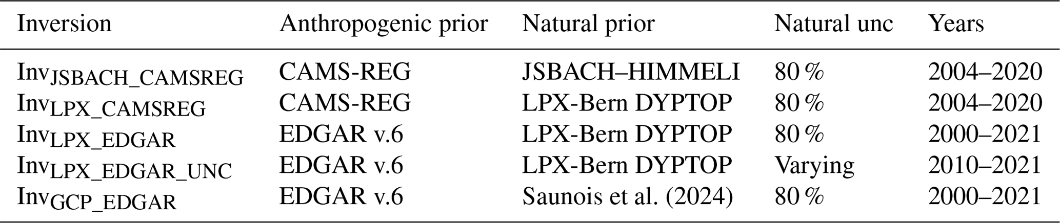
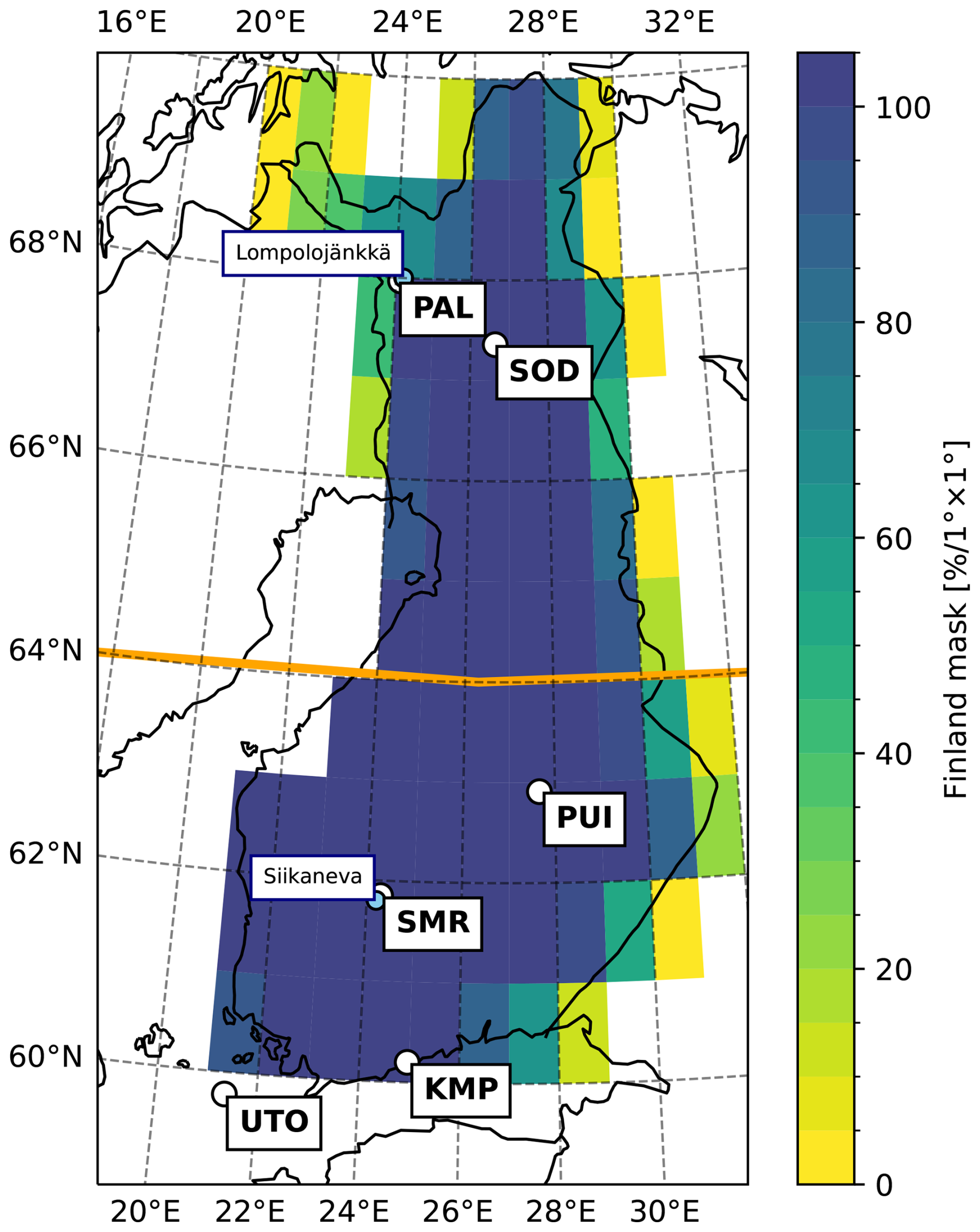
Figure 1 The land mask for Finland. Locations of six Finnish atmospheric observation sites (white dots and bold text) and flux measurement sites (blue dots). The orange line shows the boundary between southern and northern Finland.

2.3 Auxiliary CH₄ data

To help us interpret the CH₄ emissions estimated by the inverse model, we use auxiliary CH₄ datasets introduced below.

2.3.1 Ensemble of VERIFY inversions

The VERIFY project (https://verify.lsce.ipsl.fr/, last access: 12 February 2025) was a research and innovation project funded by the European Commission under the H2020 programme in 2018–2022. The project developed a GHG estimation system to support NGHGI reporting, focusing on the three major anthropogenic GHGs, namely carbon dioxide, methane and nitrous oxide. Here we use the results of the CH₄ inverse model from the VERIFY project, some of which were performed within the project, and the rest of the estimates were collected from other projects, such as the GCP (Saunois et al., 2020).

The VERIFY ensemble consists of 14 CH₄ inverse model estimates, but since one of them is Inv_{GCP_EDGAR}, we exclude it from the VERIFY ensemble as it is already included in our CTE–CH₄ ensemble. We only examine total CH₄ emissions because only 3 of the 13 VERIFY ensemble members provide the partitioning between natural and anthropogenic emissions. Three inverse model estimates do not include prior emissions estimates; there are two inversion runs with FLEXINVERT (an atmospheric Bayesian inversion framework using FLEXPART, the FLEXible PARTicle dispersion model) provided by the Norwegian research institute, NILU, and one inversion run with FLEXPART extended Kalman filter (FLExKF) provided by the Swiss institute EMPA (Swiss Federal Laboratories for Materials Science and Technology).

2.3.2 Eddy covariance CH₄ flux measurements

To verify the CH₄ emissions of the inverse model, we use eddy covariance measurements from two Finnish pristine open-peatland sites, Lompolojänkkä and Siikaneva. Lompolojänkkä (68.0° N, 24.2° E) is located in northern Finland and Siikaneva (61.8° N, 24.2° E) in southern Finland (Fig. 1). A more detailed description of Lompolojänkkä is given by Aurela et al. (2015) and of Siikaneva by Rinne et al. (2018). Eddy covariance is an atmospheric measurement technique that frequently measures vertical turbulent fluxes within the atmospheric surface layer. The footprint of the measurement, i.e. where the measured CH₄ fluxes originate, varies, depending on the prevailing meteorological conditions, but aims to cover the entire peatland ecosystem. The measurements are taken from the FLUXNET-CH₄ dataset (Delwiche et al., 2021), and the gap-filled daily values are used here to calculate monthly averages. Lompolojänkkä has data from 2006–2010 and Siikaneva from 2013–2018.

2.3.3 Freshwater CH₄ emissions

Freshwater is defined similarly to Saunois et al. (2020) here and includes lakes, ponds, reservoirs, streams and rivers. The freshwater CH₄ emission estimates examined here are from Stavert et al. (2022), who estimated the global annual freshwater CH₄ to be 53 Tg yr⁻¹.

2.3.4 Biomass-burning CH₄ emissions

The following two estimates of biomass-burning CH₄ emissions are used: GFED v4.1s (van der Werf et al., 2017), which is also used as a prior in the inversions, and the Copernicus Atmosphere Monitoring Service (CAMS) Global Fire Assimilation System (GFAS) (Kaiser et al., 2012). GFED is provided in resolutions of 0.25° × 0.25° and GFAS in resolutions of 0.1° × 0.1°. GFED has a monthly temporal resolution, and GFAS has a daily temporal resolution. We aggregate both datasets to 1° × 1° and monthly resolutions.

3 Results

3.1 Anthropogenic methane emission inventory estimates in Finland

In this section, we study the annual CH₄ emission estimates in Finland from six anthropogenic inventories. The spatial distributions of CAMS-REG, GAINS and EDGAR v7 are shown in Fig. S4.

The annual emission estimates for the four main source categories defined in the 2006 IPCC Guidelines for National Greenhouse Gas Inventories (Eggleston et al., 2006) (energy, industrial processes and product use, agriculture and waste) are shown for each inventory in Fig. 2. Of the six inventories examined, NGHGI Fi, CAMS-REG and GAINS were in good agreement (Fig. 2a). CAMS-REG used reported Finnish national data, and overall, the emissions in the two inventories had similar magnitudes and trends. The small differences between the values examined here could be explained by the fact that CAMS-REG has gridded estimates, and the values in Finland were obtained using an area mask, while NGHGI Fi is not spatially distributed. GAINS emissions were at the same level as the other two, but there were some differences; i.e. waste emissions had a larger decreasing trend and agricultural emissions were higher from 2000 to 2015. The trend in GAINS was driven by the decreasing number of cattle. This was also the case for NGHGI Fi. According to NGHGI Fi, the number of cattle decreased by more than a third between 1995 and 2021, but the decline slowed down after 2010. The decrease in the number of cattle has been offset by an increase in animal weight, growth and milk production, which has led to higher-emission factors so that the magnitude of agricultural CH₄ emissions has remained the same in recent years.

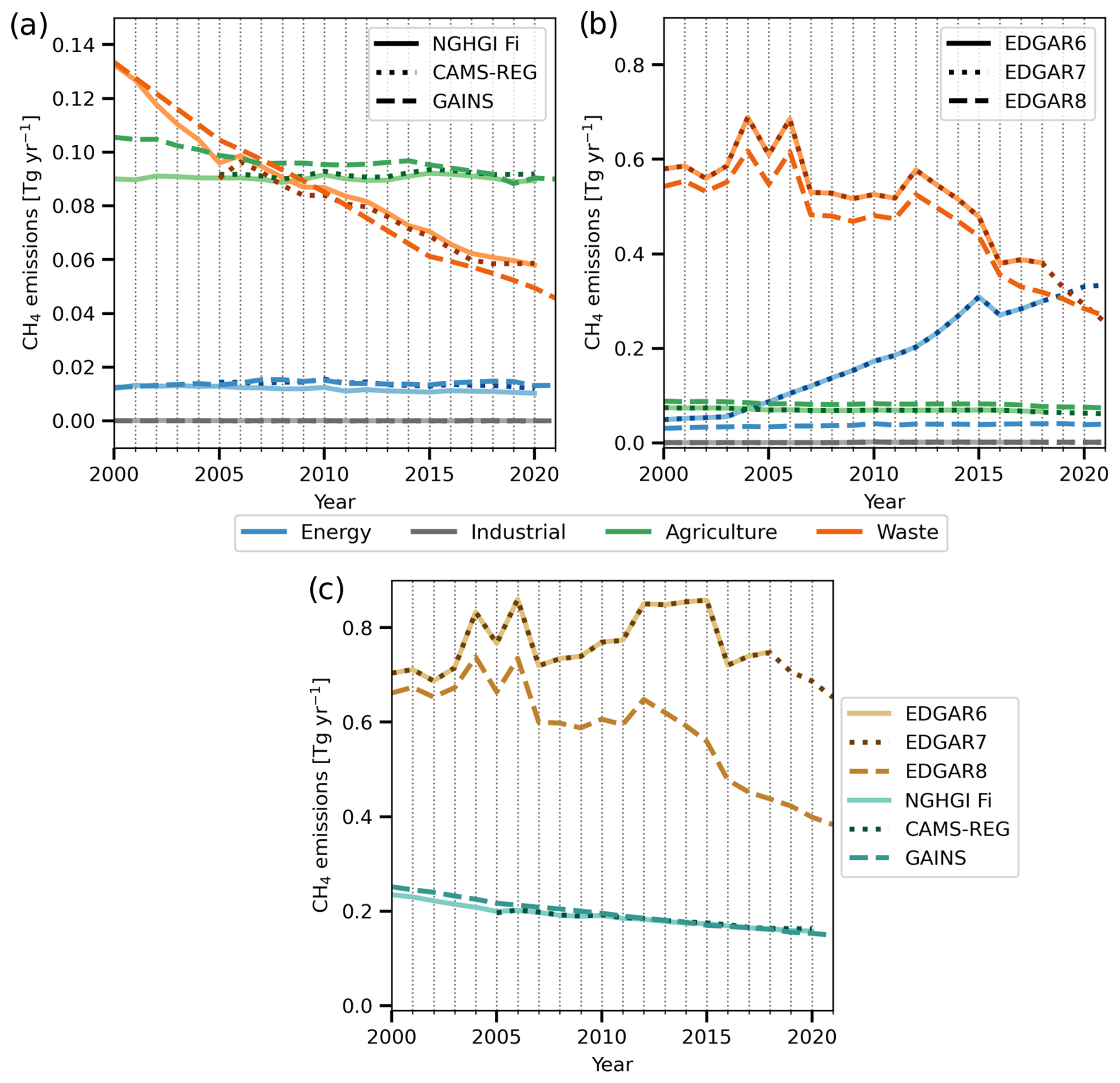
Figure 2 Annual anthropogenic CH₄ emissions per source category in Finland reported by (a) NGHGI Fi, CAMS-REG and GAINS; and (b) EDGAR v6, v7 and v8. Note the different y-axis ranges. (c) Annual total CH₄ emissions in all six inventories.

The three EDGAR versions differed from the other inventories but were similar to each other. The magnitudes of CH₄ emissions of different emission categories were the same in EDGAR v6 and v7 (Fig. 2b). The difference between the two versions was that v7 had a longer time series until 2021, while v6 ended in 2018. Agricultural and industrial emissions in all EDGAR versions were similar to those in the other inventories. Energy emissions in EDGAR v8 were lower than in v6 or v7 and showed no trend. However, the absolute magnitude was still 3 times higher in EDGAR v8 (0.03 Tg yr⁻¹) than in NGHGI Fi, CAMS-REG and GAINS (0.01 Tg yr⁻¹). In EDGAR v6 and v7, energy emissions increased significantly from 2004 onwards. This increase was due to higher estimates of fugitive methane emissions from oil refining and methane emissions from natural gas processing, transmission and distribution (Fig. S3). Waste emissions in EDGAR inventories, although decreasing over the period 2000–2021, were about 4–5 times higher than in the other inventories, although they were lower in v8 than in v6 and v7.

Waste emissions were the largest source in all inventories at the beginning of the study period. Due to the decreasing trend of waste emissions, agriculture became the largest source after 2008 in GAINS and after 2009 in NGHGI Fi. In CAMS-REG, emissions from waste were higher than those from agriculture in 2006; otherwise, agriculture had the highest emissions.

The EDGAR estimates stand out when looking at total annual emissions (Fig. 2c). While the average from 2000 to 2020 was about 0.19 Tg yr⁻¹ in NGHGI Fi and GAINS, it was 0.76 Tg yr⁻¹ in EDGAR v7 and 0.58 Tg yr⁻¹ in EDGAR v8. The EDGAR inventories also showed a higher interannual variability, especially in the waste sector, than the other inventory estimates.

3.2 Atmospheric inverse model emission estimates in Finland

3.2.1 Annual estimates from CTE–CH₄

In this section, we study the annual total, anthropogenic and natural CH₄ emissions in Finland and how the posterior emissions differed from the prior emissions, depending on the inverse model setup. The spatial distribution of the prior and posterior emissions is shown in Figs. S4–S7.

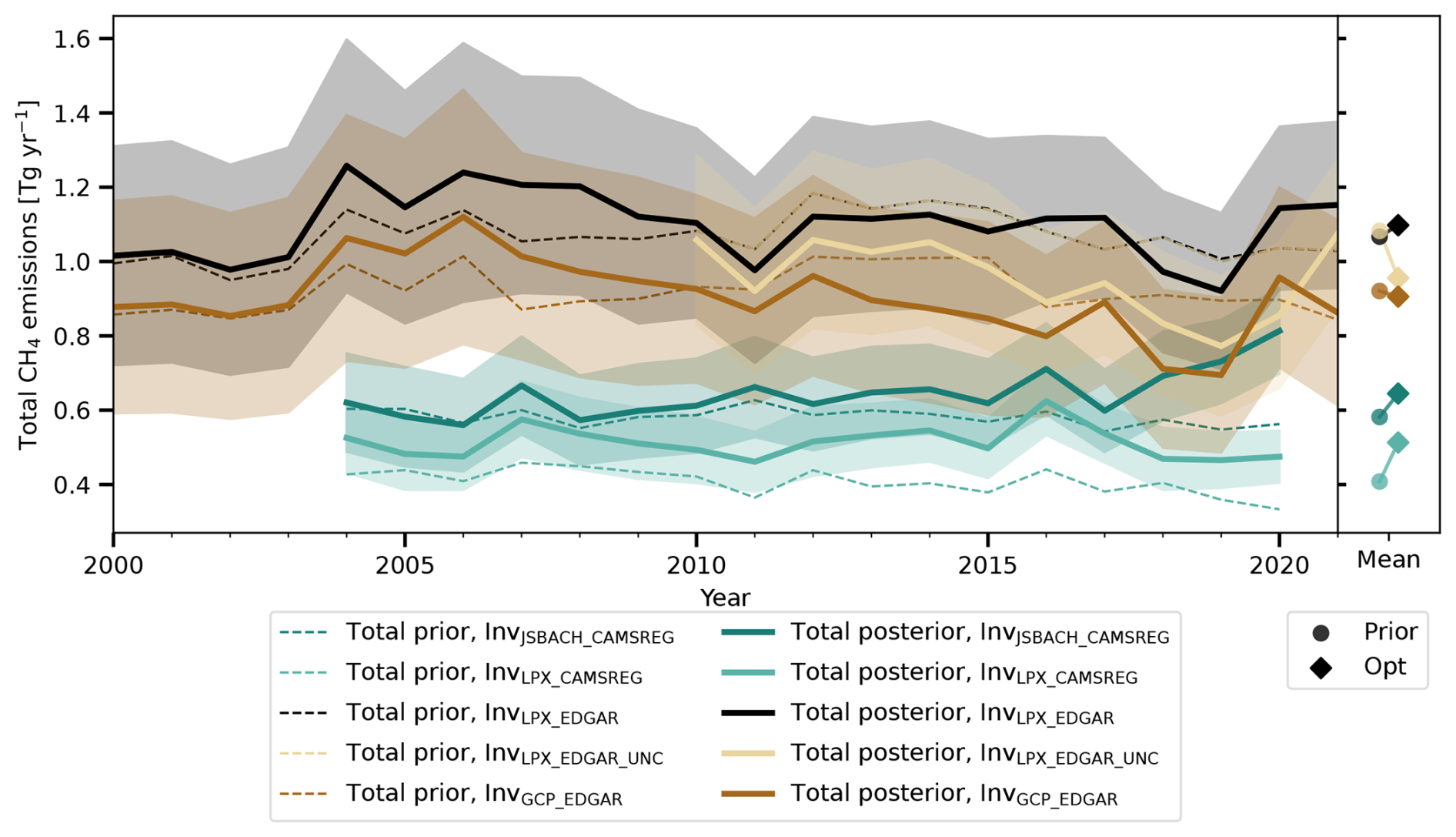
Figure 3 Annual total CH₄ emission estimates from the five CTE–CH₄ runs. Prior emissions are shown as dashed lines, and posterior emissions are shown as solid lines. The shaded areas around the posterior emissions show 1 standard deviation of the ensemble distributions. The right panel shows the mean prior and posterior emissions over the study period.

The annual total emissions of Finland from the five CTE–CH₄ inverse model runs are shown in Fig. 3. The prior emissions evidently had a strong influence on the posterior emissions. The range of the total prior emissions was large, but the range of the optimised emissions was smaller after 2009 and until 2020, with an average range of 0.57 Tg yr⁻¹ in 2009–2020, while the range of the prior emissions was 0.69 Tg yr⁻¹ in the same period. The inversions using LPX-Bern DYPTOP as the natural prior estimates had the highest (Inv_{LPX_EDGAR}; 1.1 Tg yr⁻¹ on average) and lowest (Inv_{LPX_CAMSREG}; 0.51 Tg yr⁻¹ on average) total emission estimates, while the three estimates between them agreed well, especially after 2016. To better explain the differences between the total emission estimates, the anthropogenic and natural CH₄ emissions are studied separately below.

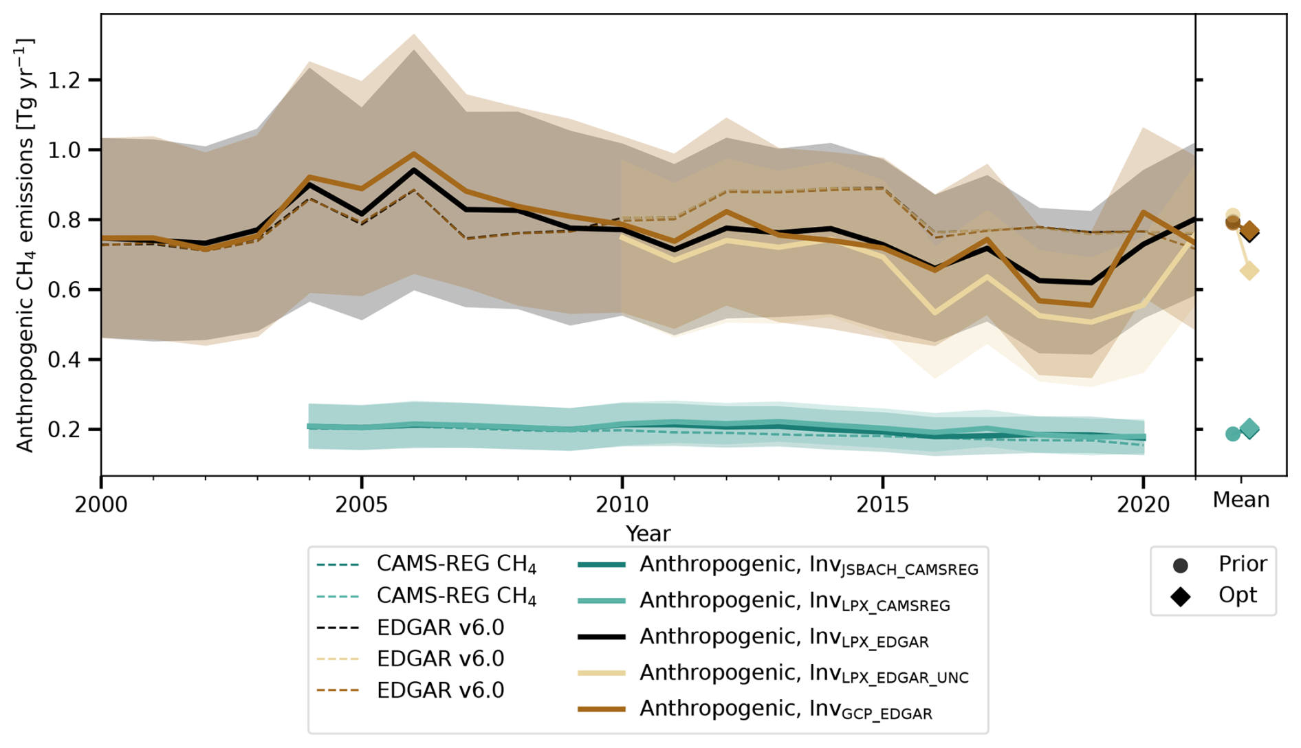
Figure 4 Annual anthropogenic CH₄ emission estimates from the five CTE–CH₄ inverse model runs. Prior emissions are shown as dashed lines and posterior emissions as solid lines. The shaded areas around the posterior emissions show 1 standard deviation of the ensemble distributions. The right panel shows the mean prior and posterior emissions over the study period.

The magnitudes of the two anthropogenic posterior emission estimates using CAMS-REG were similar and slightly higher than CAMS-REG (Fig. 4). The optimised results using EDGAR v6 varied more, but all posterior emissions were higher than EDGAR v6 until 2009 and lower thereafter until 2020 or 2021, bringing the posterior estimates of the five inversions closer together compared to their prior estimates. The two anthropogenic posterior emissions using EDGAR v6 combined with the default uncertainty estimate for the natural prior (Inv_{LPX_EDGAR} and Inv_{GCP_EDGAR}) had similar anthropogenic emission estimates, but the inversion with varying uncertainty estimates for the natural prior (Inv_{LPX_EDGAR_UNC}) had lower optimised anthropogenic emission estimates than the other two, especially after 2016.

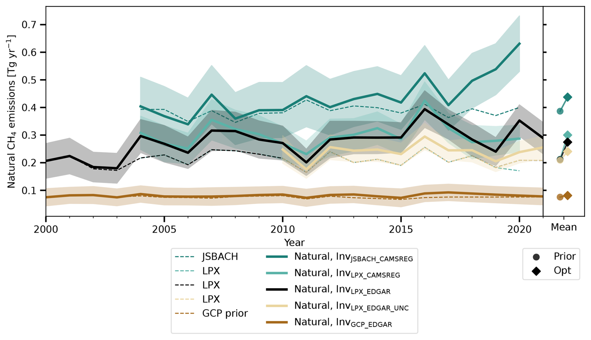
Figure 5 Annual natural CH₄ emission estimates from the five CTE–CH₄ inverse model runs. Prior emissions are shown as dashed lines and posterior emissions as solid lines. The shaded areas around the posterior emissions show 1 standard deviation of the ensemble distributions. The right panel shows the mean prior and posterior emissions over the study period.

The natural posterior emissions were always higher than the prior used, regardless of the natural prior, except in 2005 and 2006 when JSBACH–HIMMELI was higher (Fig. 5). The order of the emission estimates was also maintained after optimisation; the posterior emissions of Inv_{JSBACH_CAMSREG} were the highest, and Inv_{GCP_EDGAR} were the lowest. The three posterior emissions using LPX-Bern DYPTOP as a prior lay between these two estimates, with the inversion using the prior uncertainty estimates based on the ensemble of process-based models (Inv_{LPX_EDGAR_UNC}) giving the lowest estimates of the three. Since the estimates using the GCP prior did not change much, but the optimised emissions with JSBACH–HIMMELI were increased, the range of natural posterior emissions (0.08–0.44 Tg yr⁻¹) was larger than the range of prior emissions (0.08–0.39 Tg yr⁻¹).

Table 3 Linear trends [Gg yr⁻¹] and their p values (in brackets) for anthropogenic, natural and total CH₄ emission estimates in Finland. Values for prior and optimised estimates from the five CTE–CH₄ inversion runs are shown. Statistically significant trends (p value smaller than 0.05) are bolded.

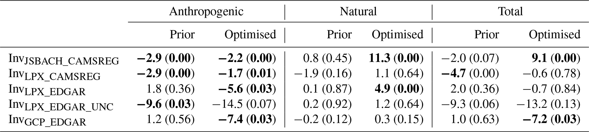
Even though the absolute magnitudes of total CH₄ emissions and the partition between anthropogenic and natural emissions differed between inversion runs, the trends of the emission estimates were more similar after the optimisation (Table 3). All anthropogenic posterior emissions had decreasing trends, although there was no significant trend in EDGAR v6 for 2000–2021. Similarly, there were no significant trends in the natural prior emissions, but there were small positive trends in the optimised natural emissions with Inv_{JSBACH_CAMSREG} (0.01 Tg yr⁻¹; p value 0.0003) and Inv_{LPX_EDGAR} (0.005 Tg yr⁻¹; p value 0.004). Decreasing anthropogenic emissions and increasing natural emissions cancelled each other out so that the only statistically significant trends in total emissions were found in Inv_{GCP_EDGAR} (−0.007 Tg yr⁻¹; p value 0.03) and Inv_{JSBACH_CAMSREG} (0.009 Tg yr⁻¹; p value 0.001). The signs of the trends were opposite, reflecting the partitioning between natural and anthropogenic emissions; Inv_{GCP_EDGAR} had the highest anthropogenic emissions and the lowest natural emissions, while Inv_{JSBACH_CAMSREG} had the highest natural emissions and the lowest anthropogenic emissions.

3.2.2 Years 2020 and 2021

During the last 2 years of the study period, 2020–2021, the growth rate of the global atmospheric CH₄ was remarkably high (Lan et al., 2024; Nisbet et al., 2023). Although our inversion results did not show exceptionally high CH₄ emissions during this period, there were still some consistent signals from the inversion estimates. In 2020, all total posterior emissions were higher than in 2019. This increase was due to increases in both anthropogenic and natural emissions, except for Inv_{GCP_EDGAR}, where the increase was due to anthropogenic emissions alone. However, its natural prior and posterior emissions were low compared to the other estimates. In contrast to Inv_{GCP_EDGAR}, the natural posterior emissions using JSBACH–HIMMELI as the natural prior (Inv_{JSBACH_CAMSREG}) were highest in 2020.

In 2021, there were only three posterior emission estimates, namely Inv_{LPX_EDGAR}, Inv_{LPX_EDGAR_UNC} and Inv_{GCP_EDGAR}. The three optimised total emissions were still higher than in 2019, but emissions from Inv_{GCP_EDGAR} were lower in 2021 than in 2020, while inversions with LPX-Bern DYPTOP were higher in 2021. The partitioning to natural or anthropogenic was also inconsistent across the three inversion estimates; Inv_{GCP_EDGAR} had lower anthropogenic and natural emissions in 2021 than in 2020, while in Inv_{LPX_EDGAR_UNC} it was the other way round. At the same time, the anthropogenic emissions of Inv_{LPX_EDGAR} were higher, and the natural emissions were lower in 2021 than in 2020. However, the differences between 2021 and 2020 were similar in magnitude to previous years.

In 2021, all estimates were higher than the prior total emissions, and in particular, the anthropogenic posterior estimates were close to the anthropogenic prior estimates. Part of the reason for this may be due to the high biomass-burning emissions in GFEDv4.1s, which seemed to affect at least the emissions in Inv_{LPX_EDGAR_UNC}. The natural posterior emission estimates of Inv_{LPX_EDGAR_UNC} in high northern latitudes (north of 50° N) were substantially higher than the emissions from LPX-Bern DYPTOP in 2016–2020, but in 2021, the emissions decreased by 15 Tg compared to 2020 (Fig. S8). CH₄ emissions of GFED in the high northern latitudes were 8.6 Tg in 2021 compared to 3.3 Tg yr⁻¹ in 2016–2020 (Fig. S9). The high emissions from biomass burning in the high northern latitudes most likely also affected the methane budget estimates in Finland, although there were no major forest fires in Finland. Emission estimates from another biomass-burning dataset, GFAS, were also high in 2021 but only about half of the GFED estimates (4.9 Tg; Fig. S9).

3.2.3 Comparison of CTE–CH₄ and VERIFY ensembles

We also compared the CTE–CH₄ emission estimates with the inversion results from the VERIFY project (Fig. 6). In the CTE–CH₄ ensemble, the average of the total CH₄ emissions from 2000–2021 was 0.83 Tg yr⁻¹ (average minimum and maximum range was 0.51–1.10 Tg yr⁻¹) in the prior and 0.85 Tg yr⁻¹ (0.59–1.08 Tg yr⁻¹) in the posterior estimates. In the VERIFY ensemble, the prior emissions were 1.50 Tg yr⁻¹ (0.78–2.28 Tg yr⁻¹), almost twice that of the CTE–CH₄ ensemble, but the posterior emissions were reduced to 0.98 Tg yr⁻¹ (0.61–1.43 Tg yr⁻¹), bringing the total CH₄ emission estimates close to the CTE–CH₄ ensemble and within the range of the posterior CTE–CH₄ ensemble estimates. The ranges of the posterior emission were large, but the range was considerably smaller than the range of the prior estimates. The lowest posterior emissions from both ensembles were approximately 0.6 Tg yr⁻¹, but the highest emissions differed by 0.3 Tg yr⁻¹.

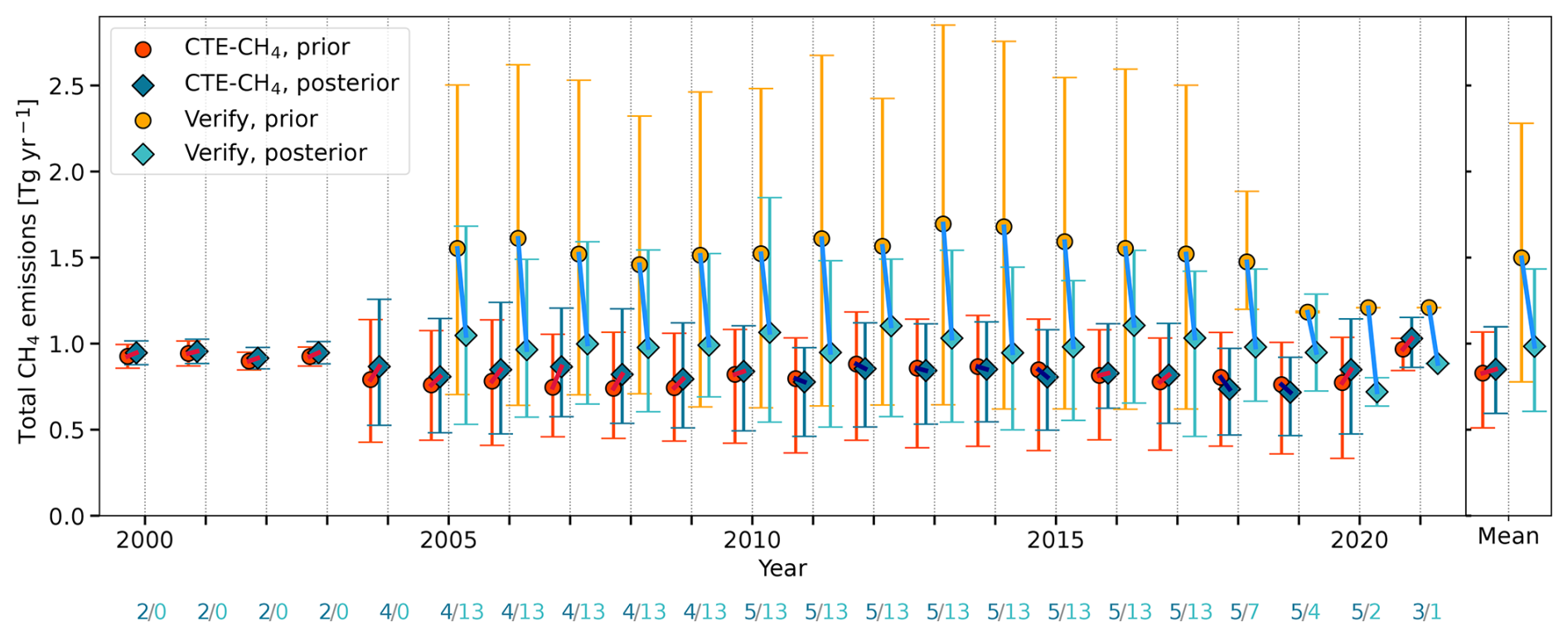
Figure 6 Estimated total annual CH₄ emissions in Finland in 2000–2021, using inverse models. Two ensembles are included, namely CTE–CH₄ and VERIFY. The circle (prior) and diamond (optimised) symbols indicate the ensemble means. The lowest- and highest-emission estimates are indicated by the lower and upper ends of the bars. Values for the priors are shown in yellow (VERIFY) and red (CTE–CH₄), and values for the optimised estimates are shown in light blue (VERIFY) and dark blue (CTE–CH₄). The mean values of the priors are connected to the mean values of the posteriors by a line. The colour of the line indicates whether emissions have increased (red) or decreased (blue) compared to the prior. The number below the year gives the number of ensemble members in the CTE–CH₄ (dark blue) and VERIFY (light blue) ensembles for that year. The right panel shows the mean values over the whole study period.

3.3 Seasonal cycle of methane emissions

Methane emissions, especially those from natural sources, have a strong seasonal cycle, and in addition to estimating the magnitude of emissions, it is important to have a correct estimate of the timing of CH₄ emissions. We calculated the monthly CH₄ emissions to see how the optimisation affected the seasonal cycle. Since the climate in southern and northern Finland is different, and thus the timing of natural CH₄ emissions in southern and northern Finland also differs, we divided the emissions from 64° N according to the division used, for example, in the Finnish NGHGI (Fig. 1). We focused on studying the emissions during the common time period between all inversion runs (2010–2020).

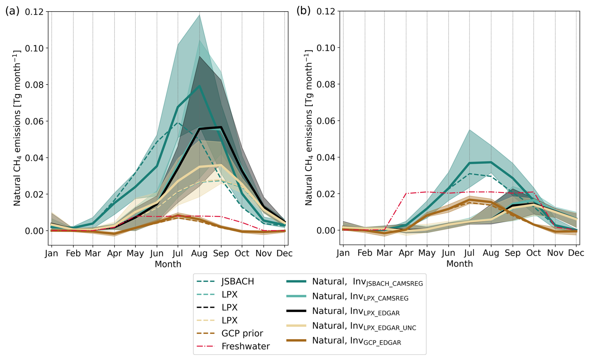
Figure 7 Average monthly natural CH₄ emission estimates from the five CTE–CH₄ inverse model runs in (a) northern and (b) southern Finland in 2010–2020. Prior estimates are shown as dashed lines, and optimised estimates are shown as solid lines. The shaded areas show the minimum and maximum monthly posterior emission estimates. Freshwater emissions from Stavert et al. (2022) are shown with dashed–dotted red lines.

The average, maximum and minimum monthly optimised natural emissions and the average of the prior emissions in 2010–2020 are shown in Fig. 7. There was a clear difference between the natural emissions in northern and southern Finland, as the maximum monthly emission estimate was almost 0.12 Tg per month in the north and only half of that in the south. In addition, the timing of the maxima of the posterior emissions differed between the south and the north, whereas the maxima in the priors were different only in the LPX-Bern DYPTOP; in LPX-Bern DYPTOP, the maximum was either in August or September in the north and in September or October in the south, while in JSBACH–HIMMELI and the natural prior GCP, the maximum was always in July. In northern Finland, the maximum of Inv_{GCP_EDGAR} emissions did not change from July, but the maximum of Inv_{JSBACH_CAMSREG} emissions was in August rather than in July. In southern Finland, the timing of the emissions did not change much from the priors, except for Inv_{JSBACH_CAMSREG}, where the posterior emissions were slightly shifted towards late summer.

In northern Finland, the posterior emissions using LPX-Bern DYPTOP (Inv_{LPX_CAMSREG}, Inv_{LPX_EDGAR} and Inv_{LPX_EDGAR_UNC}) had the largest increase from the priors in July to September so that the maximum was also shifted earlier towards late summer, although September was still the maximum in half of the years (Fig. 7a). This shift was less pronounced in Inv_{LPX_EDGAR_UNC}. The relative uncertainty estimates of the natural prior emissions in Inv_{LPX_EDGAR_UNC} varied monthly and were defined independently for each 1° × 1° grid cell in Finland. This meant that whether the assigned uncertainty was larger or smaller than the constant 80 % used in the other inversions also depended on the month and location. From November to January, the uncertainty was smaller almost everywhere in Inv_{LPX_EDGAR_UNC} compared to Inv_{LPX_EDGAR}. In February and March, Inv_{LPX_EDGAR_UNC} and Inv_{LPX_EDGAR} had low natural prior CH₄ emissions and small uncertainties. From April to June, the uncertainty in Inv_{LPX_EDGAR_UNC} was larger in northern Finland and smaller in southern Finland, but this did not have a strong effect on the posterior emissions, which remained close to the prior (Fig. 7a). From July to October, the uncertainty in the north was much smaller in Inv_{LPX_EDGAR_UNC} than in the other inversions, especially in grid cells where the natural prior emissions were high. Thus, the optimisation was more constrained by the prior than when the default uncertainty was used. However, southern Finland had a larger uncertainty in summer and autumn. As the optimisation had more freedom to adjust the CH₄ emissions in southern Finland in Inv_{LPX_EDGAR_UNC}, it could also give more weight to the observation in the south. The natural posterior CH₄ emissions in the south did not differ between Inv_{LPX_EDGAR_UNC} and Inv_{LPX_EDGAR}, but the anthropogenic posterior emissions were lower in Inv_{LPX_EDGAR_UNC} than in Inv_{LPX_EDGAR}, especially in July–October (Fig. S10). The lower natural emissions in the north and anthropogenic emissions in the south resulted in lower total emissions in Inv_{LPX_EDGAR_UNC} compared to Inv_{LPX_EDGAR}, and brought the seasonal cycle of total CH₄ emissions of Inv_{LPX_EDGAR_UNC} close to the seasonal cycle of Inv_{JSBACH_CAMSREG} (Fig. 8a).

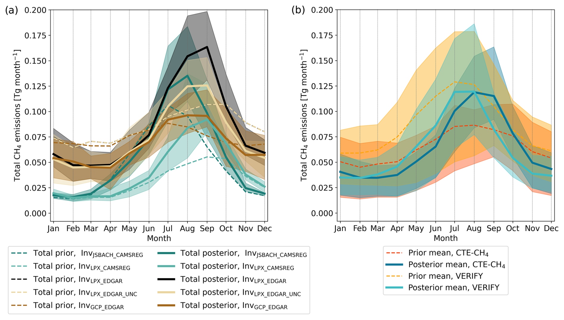
Figure 8 (a) Average monthly total CH₄ emission estimates from the five CTE–CH₄ inverse model runs in Finland from 2010–2020. Prior estimates are shown as dashed lines, and optimised estimates are shown as solid lines. The shaded areas show the lowest and highest monthly posterior emission estimates. (b) Average of the monthly total CH₄ emission estimates from the CTE–CH₄ and VERIFY ensembles in Finland from 2010–2020. The shaded areas show the minimum and maximum monthly estimates.

A comparison of the seasonal cycles of the total CH₄ emissions between the CTE–CH₄ and VERIFY ensembles (Fig. 8b) shows similar results to the comparison of the annual totals; the VERIFY prior emissions were higher on average and had a wider range than the prior emissions in the CTE–CH₄ ensemble, but the amplitudes of the seasonal cycles of the average posterior emissions agreed well. However, the phases of the average posterior emissions differed; the VERIFY ensemble was consistently 1 month ahead of the CTE–CH₄ ensemble.

Figure 7 also shows the freshwater CH₄ emissions from Stavert et al. (2022). These emissions were not included in the prior emissions of Inv_{GCP_EDGAR} or in the other inversions. In northern Finland, the estimated freshwater emissions were considerably lower than the posterior natural emission estimates (except for Inv_{GCP_EDGAR}), but in southern Finland, where there are many shallow lakes, they were almost as high as the posterior natural emissions; the freshwater emissions were 0.15 Tg yr⁻¹, while the JSBACH–HIMMELI emissions were 0.13 Tg yr⁻¹, and the optimised natural emissions in Inv_{JSBACH_CAMSREG} were 0.16 Tg yr⁻¹ on average in 2010–2020.

We also compared the seasonal cycles of the natural emission estimates with flux measurements from two Finnish pristine peatlands. Figure 9 shows the measured CH₄ fluxes from Lompolojänkkä (northern Finland) and Siikaneva (southern Finland). At Lompolojänkkä, the different years had very similar seasonal cycles, and the maximum was in August, except in 2008 when the maximum was in July. At Siikaneva, CH₄ fluxes varied more from year to year. Nevertheless, the maximum of the fluxes was relatively consistent regarding being in July or in August. In both peatlands, July and August were the months with the highest CH₄ fluxes. Due to the alterations made by the inverse model, the seasonal cycles of the optimised emission estimates were more consistent with the flux measurements than the seasonal cycles of the prior estimates. However, it should be noted that the inverse model estimates aggregate much larger areas and a variety of sources rather than a single peatland, so a direct comparison between the flux measurements and the inverse model results is not possible.

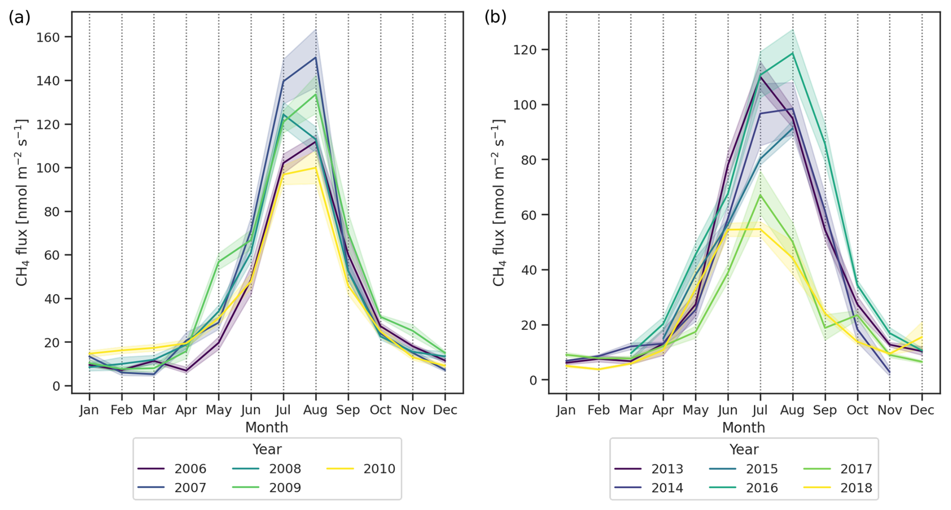
Figure 9 Average monthly CH₄ flux measurements at (a) Lompolojänkkä (northern Finland) and (b) Siikaneva (southern Finland). The shaded areas show a 95 % confidence interval.

3.4 Comparison of modelled methane mole fractions to observations in Finnish sites

The CH₄ emission estimates in Finland varied, depending on the priors and prior uncertainty estimates used. To understand which inversion best estimated CH₄ emissions in Finland, we compared modelled and observed mole fractions at the six Finnish in situ sites also used in the optimisation. We examined only the years 2010–2020, as these were common to all inversion runs. Observations from Utö were included from March 2018 and Hyytiälä from December 2016 as all inversions included observations from these two sites. The effect of including all available years was also examined, but it did not change the result significantly. In addition to the optimised mole fractions, we also studied the mole fractions modelled with the prior emissions using a so-called forward run mode, i.e. using only the TM5 transport model without the data assimilation. The term “prior” refers to these modelled mole fractions in this section. Similarly, the term “posterior” is used to refer to the mole fractions obtained using the optimised emissions.

In Fig. 10, correlation coefficients, detrended root mean square errors (RMSE) and standard deviations are shown as Taylor's diagrams (Taylor, 2001) for all Finnish sites, comparing both the prior and posterior mole fractions. The correlation coefficient describes the linear relationship between the modelled and observed mole fractions, with values close to 1 indicating good agreement between the two. The detrended RMSE quantifies and summarises the differences between the modelled and observed mole fractions. From the RMSE alone, it is not possible to determine whether the differences are due to different phases in the datasets or due to differences in the amplitudes of the variations. The standard deviation provides additional information and shows how much variation there is in each dataset.

The statistics of the priors varied more than the statistics of the posterior mole fractions (Fig. 10; see also Fig. S11). The prior values of Inv_{GCP_EDGAR} were in better agreement with the observations than the other priors at almost all observation sites, especially at PUI, SMR and PAL. However, in contrast to the other inverse model setups, the posterior statistics of Inv_{GCP_EDGAR} improved only slightly from the priors at PAL and SOD, which are two northern stations surrounded by natural CH₄ sources. Overall, the posterior mole fraction from different inverse model runs showed similar statistics, especially at the UTO and SMR stations.

To summarise the statistics of the optimised mole fractions, we ranked selected statistics as follows: for each site and inversion run, the bias, the detrended RMSE and the detrended linear correlation coefficient R were calculated. The bias was used instead of the standard deviations in Taylor's diagrams to emphasise any systematic errors in the modelled mole fractions. Detrending the data removes long-term variations and allows us to examine short-term variations. We detrended the data using the method introduced by Thoning and Tans (1989), which takes a seasonal cycle into account. The absolute value of each variable was then ranked between the inversion runs from one to five, with the smallest being the best value for the bias and the detrended RMSE and the largest being the best value for the detrended R. The average of the three rankings for each inversion run, as well as the average of all six stations, is shown in Fig. 11. The same figure, but with prior statistics, is shown in Fig. S11.

Based on the average rankings, there was no single inversion setup that stood out as the best across all sites. Most inversion runs had better and worse rankings, depending on the site. However, Inv_{LPX_EDGAR_UNC} had the best rankings in general (average 2.11), especially in the southern sites (UTO, KMP and SMR). In the northern sites (PAL and SOD), where natural CH₄ sources dominate, Inv_{JSBACH_CAMSREG} had the best rankings. Inv_{JSBACH_CAMSREG} also had the second-best overall ranking (2.61). The seasonal cycles of the optimised total CH₄ emissions of Inv_{LPX_EDGAR_UNC} and Inv_{JSBACH_CAMSREG} were also quite similar (Fig. 8a). Inv_{GCP_EDGAR} had the best rankings in PUI and SMR, where the prior statistics already showed good agreement with the observations, but the worst rankings in the northern peatland sites. Inv_{LPX_CAMSREG}, which had the lowest total posterior emissions, had the worst rankings in general, and Inv_{LPX_EDGAR}, which had the highest total posterior emissions, had average rankings across all sites.

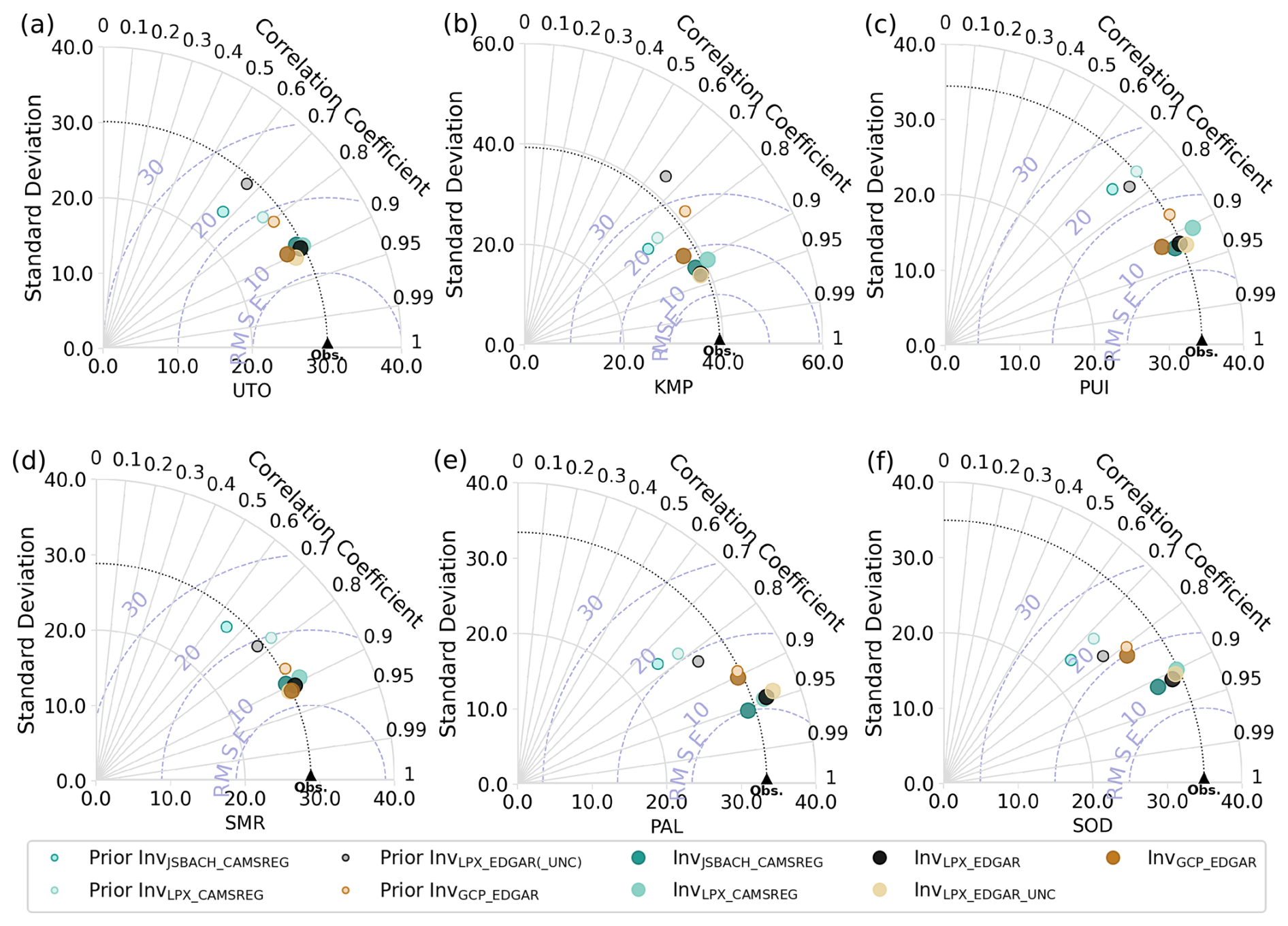
Figure 10 Taylor's diagram of the results of the five CTE–CH₄ inverse model runs against the measured mole fractions from the Finnish stations. (a) UTO, (b) KMP, (c) PUI, (d) SMR, (e) PAL and (f) SOD. Smaller circles correspond to values from forward modelling results using the TM5 transport model and prior emissions. The prior values of Inv_{LPX_EDGAR_(UNC)} are the same for Inv_{LPX_EDGAR} and Inv_{LPX_EDGAR_UNC} as they had the same prior emissions.

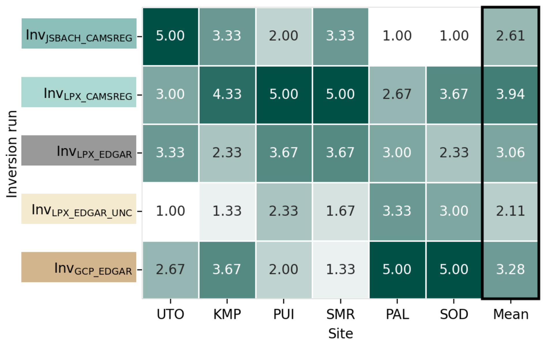
Figure 11 The average rank calculated for each inverse model run for each site is shown. The bias, detrended RMSE and detrended R of the modelled and measured mole fractions were calculated with each inversion model run in each site, and the values were then ranked between the model estimates (the lowest being the best in bias and RMSE and the highest being the best in R). In addition, the rightmost column is the average of all site averages.

4 Discussion

4.1 Total methane emission estimates

We estimated methane emissions in Finland using the atmospheric inverse model CTE–CH₄. As a global model, it was able to constrain the global total emissions well (on average 525 Tg yr⁻¹, with a minimum and maximum range of 3.2 %). However, the ratio of the range to the average total emissions in Finland was much larger at 58 % (71 % in the priors), which shows the difficulty of constraining emissions at the country level and also how the underlying prior emissions and their distribution affect emission estimates at a smaller scale. Nonetheless, using a global model, the optimisation of emissions in a region of interest is not separated from the emissions that occur outside of the region.

The range of posterior CH₄ emissions in Finland was large in the VERIFY ensemble (Fig. 6), which included estimates from different inverse models and model runs, some of which used the same priors and observations, and some of which had their own setups. The range of prior estimates was even wider, and as the optimisation always reduced the estimates, the highest prior estimates were most likely too high. Furthermore, the highest CTE–CH₄ estimate (Inv_{LPX_EDGAR}), which was lower than the highest estimate in the VERIFY ensemble, showed only moderate agreement with atmospheric CH₄ observations, indicating that CH₄ emissions were probably too high. Thus, the CTE–CH₄ ensemble range seemed more reliable, especially when excluding its highest estimate. Although the ranges of posterior emissions were large, the averages of the VERIFY and CTE–CH₄ ensembles were in good agreement. This is consistent with previous model intercomparisons which have shown that inversions can constrain emissions on a larger scale and that ensembles of inverse model estimates are more reliable and robust than estimates from a single inversion run (Petrescu et al., 2024; Saunois et al., 2020; Stavert et al., 2022). Further partitioning into independent countries still relies on the distributions of the priors.

4.2 Partition to anthropogenic and natural emissions

When comparing CH₄ estimates from the inverse model with national GHG inventories, it is important to understand not only the total CH₄ budget but also the partitioning of emissions reported in the inventories. As these inventories only cover anthropogenic activities, the share of anthropogenic emissions in the total CH₄ estimates is particularly important. In CTE–CH₄, emissions from anthropogenic and natural sources were optimised separately but simultaneously. The emissions from both categories were analysed as they were refined by CTE–CH₄.

The anthropogenic emission inventories gave two drastically different estimates of Finnish CH₄ emissions, with EDGAR v6, v7 and v8 giving much higher estimates than the other three, namely NGHGI Fi, CAMS-REG and GAINS (Fig. 2c). Olhoff et al. (2022) compared the NGHGI estimates with EDGAR v6 in the Nordic countries and showed that the CH₄ estimates from EDGAR v6 were much higher than the NGHGI estimates from Finland, Norway and Sweden. They showed that the discrepancies were due to fugitive emissions (in Norway and Finland) and waste emissions (in Sweden and Finland). In addition, using Bayesian inverse modelling, Worden et al. (2022) estimated Finland's waste emissions to be 0.11 ± 0.29 Tg in 2019 instead of the prior value of 0.60 ± 0.36 Tg (EDGAR v4.3.2 in 2012), which is much more consistent with the NGHGI Fi (0.06 Tg). Saboya et al. (2022) compared modelled mole fractions using an older version of EDGAR (v4.3.2) with observations in London and found that emissions from the waste sector were high and inconsistent with their estimates. As a global product, EDGAR uses globally consistent methodologies, meaning country-specific mitigation strategies may not have been considered. For example, fugitive emissions from the oil and gas sector in EDGAR v6 followed the trend of activity data in the Nordic countries, indicating that efforts to reduce emissions were not taken into account (Janssens-Maenhout et al., 2019; Olhoff et al., 2022). However, in the latest update of EDGAR v8 (European Commission and Joint Research Centre et al., 2023), there seems to be an improvement in the estimates for the energy sector, as they show the same trend as the other inventories in Finland (Fig. 2c).

Based on the comparison between atmospheric mole fractions modelled with CTE–CH₄ and observations from Finnish sites, neither EDGAR v6 nor CAMS-REG seemed to be better than the other (Fig. 11). As the comparison with the atmospheric mole fraction does not directly provide information on whether the split between anthropogenic and natural emissions is correct, this may indicate that the inverse model had difficulties in separating anthropogenic and natural emissions. This is particularly likely in southern Finland, where there are anthropogenic and natural CH₄ sources. It may also reflect the complexity of modelling urban fluxes. To improve estimates of anthropogenic emissions, it would be interesting to combine city-scale estimates with our larger-scale inversions.

The three natural CH₄ priors used in this study differed in absolute magnitude and in spatial and temporal distribution. The comparison with the atmospheric observations from northern Finland gave a clear ranking of the three priors. Inv_{JSBACH_CAMSREG}, with the highest emission estimates, seemed to have the most accurate natural estimates in Finland; inversion runs with LPX-Bern DYPTOP had the second-best ranking; and Inv_{GCP_EDGAR}, with the lowest emission estimates, had the worst ranking (Fig. 11). The natural posterior emissions were always higher than their priors, even from JSBACH–HIMMELI, and the largest increases were in 2016, when the summer was warm and rainy (Finnish Meteorological Institute, 2016), and in 2019–2020 (Fig. 5). Our results indicate that Finnish natural CH₄ emissions from peatlands might be underestimated by the process-based models, although the high natural posterior emissions could also be due to sources other than peatlands. In particular, emissions from freshwater sources are relevant. We compared the freshwater emission estimates from Stavert et al. (2022) with the natural CH₄ prior and posterior emissions in Fig. 7 and showed that in southern Finland these estimates were as high as the highest optimised natural emissions (Inv_{JSBACH_CAMSREG}). The spatial distribution of the freshwater emission estimates coincided with the JSBACH–HIMMELI estimates (Fig. S12), so the inversion would most likely have included freshwater emissions in the posterior natural emission estimates. However, as there were still methane-emitting peatlands in southern Finland, it is not expected that optimised Inv_{JSBACH_CAMSREG} emission estimates would have included only freshwater emissions. Therefore, the freshwater emission estimates in Finland seemed to be too high.

4.3 Years 2020 and 2021

The reasons for the high atmospheric CH₄ growth rates in recent years, especially in 2020–2021, have been under discussion. Part of the high growth rate in 2020 has been attributed to a weaker OH sink caused by a decrease in NO_x emissions due to the COVID-19 lockdowns (Stevenson et al., 2022; Qu et al., 2022; Peng et al., 2022; Feng et al., 2023). However, the weaker OH sink could not explain all of the increase in atmospheric CH₄, and wetlands, especially at high latitudes and in the tropics, were also suggested to be responsible for the increase (Qu et al., 2022; Peng et al., 2022; Zhang et al., 2023; Feng et al., 2023; Qu et al., 2024). In Finland, total CH₄ emissions were higher in 2020 than in 2019 in all CTE–CH₄ inversions, and the increase was attributed to both anthropogenic and natural emissions, but the posterior natural emissions in Inv_{JSBACH_CAMSREG}, which probably gave the most realistic estimates of natural emissions, were highest in 2020.

The increase in the CH₄ growth rate in 2021 has also been attributed to wetlands (Feng et al., 2023; Zhang et al., 2023; Qu et al., 2024). The natural CH₄ emission estimates of CTE–CH₄ in Finland were higher in 2021 than in 2019, but at the same level or lower than in 2020 (Fig. 5). To understand the Finnish emission estimates in 2021, it is beneficial to study the emissions in the whole northern high latitudes. The biomass-burning product used in the CTE–CH₄ runs, GFEDv4.1s, estimated the CH₄ emissions in the boreal forests (north of 50° N) to be 8.6 Tg, while they were 4.2 Tg in 2019 (Fig. S9). According to Feng et al. (2023), the global CH₄ emissions should have been 20.8 Tg higher in 2021 than in 2019 to reproduce the observed atmospheric methane, meaning that emissions from biomass burning in boreal forests would account for 21 % of the increase in global CH₄ emissions. Zheng et al. (2023) showed that CO₂ emissions from boreal forests have been increasing in recent decades and that CO₂ emissions were at a record high in 2021. They also used GFEDv4.1s in their analysis, but unlike our inversions, they specifically optimised biomass-burning emissions. The record-high biomass-burning CH₄ emissions in the boreal forests were probably the cause of the large decrease in the optimised wetland emissions of Inv_{LPX_EDGAR_UNC} in the high northern latitudes from 2020 to 2021 (Fig. S8). They most likely also constrained the optimisation in Finland, keeping the posterior emissions close to the prior emissions. However, to verify this, it would require further investigation and, for example, an inverse model setup in which biomass-burning CH₄ emissions are also optimised. There are also uncertainties in the biomass-burning emission estimates, and as discussed, GFAS had much lower-emission estimates north of 50° N in 2021 (4.9 Tg; Fig. S9). The increase in 2021 compared to 2019 was still relatively high in GFAS (2.2 Tg), i.e. it would have explained 11 % of the global increase in CH₄ emissions in 2021 estimated by Feng et al. (2023).

4.4 Uncertainty estimations

In addition to different prior emissions, we also investigated how different prior uncertainties affected the emission estimates in Finland. Inv_{LPX_EDGAR_UNC}, where the natural prior uncertainty was defined based on a process-based model ensemble, showed better agreement with observations at the southern sites than Inv_{LPX_EDGAR}, which used the default prior uncertainties but otherwise had the same setup (Fig. 11). In northern Finland, Inv_{LPX_EDGAR} had larger uncertainties and performed better than Inv_{LPX_EDGAR_UNC}. In addition, Inv_{JSBACH_CAMSREG}, which had the highest natural prior emissions and thus the largest uncertainties in the north, performed best at the northern sites. One might therefore expect that large uncertainties would give the optimisation the freedom to fit the posterior emissions to the observations and, with enough observations, lead to better emission estimates. However, this only seemed to be the case for natural emissions. The anthropogenic prior, EDGAR v6, had high emissions and therefore large uncertainties, so in theory, the optimisation could have reduced anthropogenic emissions more than it did. The largest reduction from EDGAR v6 was seen with Inv_{LPX_EDGAR_UNC} (Fig. 4), even though its anthropogenic prior uncertainty was the same as in the other runs. Thus, simply having large uncertainties and a relatively large number of sites does not guarantee a better estimate, but it is important to know where the uncertainties lie. It can be complicated to determine realistic uncertainty ranges, and even using an ensemble of several individual estimates may not capture the true magnitude of CH₄ emissions.

Our uncertainty estimates were based on the process-based models from the latest published GCP-CH₄ (Saunois et al., 2020). The ongoing effort to update the global CH₄ budget (Saunois et al., 2024) used an updated wetland extent product (WAD2M v2.0; Zhang et al., 2021), and 12 models had prognostic versions, almost doubling the number of model estimates from Saunois et al. (2020). It would be interesting to see how the uncertainty estimates would change if the process-based models from Saunois et al. (2024) were used.

The optimisation in our inverse model is based on the ensemble Kalman filter, which creates an ensemble of 500 members based on the priors and their uncertainties. By default, this method gives us a range of estimates that represent the uncertainties in the emission estimates. With these uncertainties we can, for example, calculate the uncertainty reduction from prior to posterior, which indicates how well the optimisation is able to constrain emissions. Another fairly robust way of estimating the uncertainties is to use different model ensembles and obtain a range of estimates (Petrescu et al., 2024; Saunois et al., 2020; Stavert et al., 2022). As shown here, using a single inverse model with different setups can constrain and produce a comparable range of CH₄ emission estimates at the country level as an ensemble of different inverse models. As it is easier for an individual researcher or research group to maintain one inverse model at a time, it would be recommended to use different priors to produce more constrained and reliable CH₄ emission estimates.

5 Conclusions

In this study, CH₄ emissions in Finland were investigated using a range of bottom-up (inventories and process-based models) and top-down (inverse models) estimates. We studied how different bottom-up emission estimates used as priors in the inverse model affected the posterior CH₄ emissions. This choice not only strongly influenced the posterior emissions but was as important as the choice of inverse model; the ensemble of inversion runs using the same inverse model, but different priors resulted in similar average total posterior emissions to using different inverse models but similar priors.

Even though the CH₄ emission estimates in Finland had a large range, the range of the total posterior emissions was smaller than the range of the prior emissions. The optimisation was also able to reconcile the trends of anthropogenic and natural CH₄ emissions, and the seasonal cycles of natural CH₄ emissions were altered by the optimisation to better match flux measurements from peatland sites. However, the spatial distributions were not radically changed from the prior emissions.

The comparison of atmospheric CH₄ observations with model results showed no clear preference between the anthropogenic inventories (EDGAR v6 and CAMS-REG), but the comparison seemed to favour the highest natural prior (JSBACH–HIMMELI). The optimised natural emissions were higher than their prior emissions, which could be due to missing emissions in the prior estimates, such as freshwater. Estimates of freshwater emissions are still highly uncertain, and the estimates examined in this study (Stavert et al., 2022) appeared to be too high for Finland. We also found evidence that CH₄ emissions from biomass burning, which were not optimised in CTE–CH₄, were likely to have a large impact on the optimised anthropogenic and natural emissions in Finland and high northern latitudes, especially in 2021. The biomass-burning emissions used in our inversions (GFEDv4.1s) had much higher emissions than those in GFAS, highlighting the uncertainties in the biomass-burning CH₄ emission estimates.

The optimised CH₄ emissions were shown to depend on the choice of prior emissions. This choice was particularly important for the optimisation of the different emission components, as the optimisation of the different emission components was based on the spatial and temporal distribution of the priors. Currently, there are six stations in Finland where atmospheric CH₄ is measured. Adding more stations would most likely help to better constrain the different emission components. In addition to more stations, we also need more reliable prior estimates and realistic uncertainty estimates. In this study, we tested an uncertainty estimate based on a process-based model ensemble for natural CH₄ emissions, which appeared to be an advantageous method compared to the standard uncertainty estimates (80 % of the prior emissions). This type of uncertainty estimation could also be used for anthropogenic emissions, although many of the anthropogenic inventories use the same statistics and activity data. However, as shown here, the choices made in compiling the inventories affect the estimated emissions, and the differences between them can help us to identify where the largest uncertainties lie.

The absolute magnitude of CH₄ emissions from Finland, especially anthropogenic emissions, is relatively small compared to global totals. Consequently, these magnitudes are primarily relevant in the context of methodological comparisons or for verifying the NGHGI. The broader relevance of this study emerges from our assessment of the ability of a global model to estimate CH₄ emissions within a single country. Such objectives are becoming increasingly relevant, as highlighted by initiatives such as the World Meteorological Organization's Global Greenhouse Gas Watch (G3W). This initiative aims to have global inverse models operationally running that could be used to assess country-specific GHG emissions. Under G3W, inverse model results will be available in common standard formats, making them more accessible and easier to use. This will likely also encourage their use in future studies by those unfamiliar with inverse models. As discussed in this study, the interpretation of inverse model results requires careful consideration of the model setup, and in particular, posterior estimates should be considered alongside prior emissions rather than as stand-alone definitive results. Ideally, those conducting the model runs would also provide uncertainty estimates (e.g. spatial and temporal uncertainty reductions from prior to posterior or an ensemble of inversions using different priors) and guidance on how to interpret the results and what factors to consider. Although the preparation of a comprehensive interpretation guide is challenging due to the possible diverse applications of model results, the establishment of some common guidelines would be beneficial (Peters et al., 2023).