Feasibility of robust estimates of ozone production rates using a synergy of satellite observations, ground-based remote sensing, and models

Ozone pollution is secondarily produced through a complex, non-linear chemical process. Our understanding of the spatiotemporal variations in photochemically produced ozone (i.e., PO₃) is limited to sparse aircraft campaigns and chemical transport models, which often carry significant biases. Hence, we present a novel satellite-derived PO₃ product informed by bias-corrected TROPOspheric Monitoring Instrument (TROPOMI) HCHO, NO₂, surface albedo data, and various models. These data are integrated into a parameterization that relies on HCHO, NO₂, HCHO $/$ NO₂, jNO₂, and jO¹D. Despite its simplicity, it can reproduce ∼ 90 % of the variance in observationally constrained PO₃, with minimal biases in moderately to highly polluted regions. We map PO₃ across various regions with respect to July 2019 at a 0.1° × 0.1° spatial resolution, revealing accelerated values (> 8 ppbv h⁻¹) for numerous cities throughout Asia and the Middle East, resulting from elevated ozone precursors and enhanced photochemistry. In Europe and the United States, such high levels are only detected over Benelux, Los Angeles, and New York City. PO₃ maxima are observed in various seasons and are attributed to changes in photolysis rates, non-linear ozone chemistry, and fluctuations in HCHO and NO₂. Satellite errors result in moderate errors (10 %–20 %) in PO₃ estimates over cities on a monthly average basis, while these errors exceed 50 % in clean areas and under low light conditions. Using the current algorithm, we demonstrate that satellite data can provide valuable information for robust PO₃ estimation. This capability expands future research through the application of data to address significant scientific questions about locally produced ozone hotspots, seasonality, and long-term trends.

1 Introduction

Tropospheric ozone (O₃) is a secondary pollutant formed through complex photochemical reactions involving various precursors, including nitrogen oxides (NO_x = NO + NO₂), volatile organic compounds (VOCs), aerosols, and halogens (Kleinman et al., 2002; Simpson et al., 2015; Li et al., 2019). Ozone not only poses significant risks to human health (Fleming et al., 2018) and agricultural productivity (Mills et al., 2018) but also influences the radiation budget, thereby affecting the climate (Gaudel et al., 2018). To mitigate the problem of elevated locally produced ozone, it is crucial to understand the spatiotemporal variability in the ozone production rate (PO₃), defined as the number of ozone molecules generated through secondary chemical pathways in the atmosphere. Comprehensive studies of ozone chemistry, informed by observations, are typically confined to observationally rich air quality campaigns (e.g., Cazorla et al., 2012; Ren et al., 2013; Mazzuca et al., 2016; Souri et al., 2020a; Schroeder et al., 2020; Brune et al., 2022; Wolfe et al., 2022; Souri et al., 2023), which are sparse in time and space.

Significant advancements have been made in using various measurable ozone indicators to simplify the non-linear relationship between PO₃, NO_x, and VOCs into linear forms (Sillman and He, 2002). These forms include NO_x-sensitive regimes (where PO₃ is sensitive to NO_x), VOC-sensitive regimes (where PO₃ is sensitive to VOCs), and transitional regimes (where PO₃ is sensitive to both NO_x and VOCs). Among the numerous proposed indicators, the ratio of formaldehyde (HCHO) to nitrogen dioxide (NO₂) (known as the FNR) has gained popularity (Tonnesen and Dennis, 2000a, b), despite its less effective performance compared to that of the H₂O₂ $/$ HNO₃ ratio in fully explaining the HO_x–RO_x cycle (Silman and He, 2002; Souri et al., 2023). The preference for the FNR stems from the fact that both HCHO and NO₂ can be informed by UV–Vis radiance data, such as those provided by the Ozone Monitoring Instrument (OMI) and the TROPOspheric Monitoring Instrument (TROPOMI) (Martin et al., 2004; Duncan et al., 2010; Choi et al., 2012; Choi and Souri, 2015a, b; Jin and Holloway, 2015; Jin et al., 2017; Schroeder et al., 2017; Souri et al., 2017; Jeon et al., 2018; Tao et al., 2022). Several limitations associated with the application of satellite-based FNRs have been identified, such as (i) the inherent limitations in understanding the radical termination in the HO_x–RO_x cycle (Souri et al., 2020a, 2023), (ii) the challenges associated with converting the column vertical density to near-surface concentrations (Jin et al., 2017; Schroeder et al., 2017; Souri et al., 2023), (iii) the spatial representativity associated with large satellite pixels (Souri et al., 2020a, 2023; Johnson et al., 2023), and (iv) retrieval errors (Souri et al., 2023; Johnson et al., 2023). Souri et al. (2023) concluded that retrieval errors make up the largest portion of the total errors associated with FNRs. These errors are becoming smaller with improved sensor designs, retrieval algorithms, and calibration over time.

While the characterization of ozone regimes offers valuable insights for regulators to prioritize effective emission control strategies, it does not provide information about the magnitude of PO₃ or the absolute quantities of PO₃ derivatives relative to its precursors. Consequently, chemical transport models under various emission scenarios are typically employed (e.g., Pan et al., 2019). These models allow for the execution of process-based scenarios to elucidate the response of PO₃ to different emissions and can simulate four-dimensional PO₃ data. However, the results of these simulations are based on various assumptions and inputs, which carry significant uncertainties. Therefore, it is essential to optimize some of the models' prognostic inputs using observations through inverse modeling/data assimilation. The primary advantage of inverse modeling/data assimilation using satellite observations is its ability to account for satellite errors and eliminate the influence of the a priori profile, thereby carrying only radiance information into the emission estimation. Numerous studies have utilized satellite observations to constrain NO_x and VOC emissions for various applications (e.g., Stavrakou et al., 2016; Souri et al., 2016a; Miyazaki et al., 2017; Souri et al., 2017, 2020b, 2021; Choi et al., 2022; DiMaria et al., 2023). Souri et al. (2020b) made an early attempt to simultaneously optimize both NO_x and VOC emissions over eastern Asia for a more accurate representation of PO₃. Their joint inversion was able to account for the intertwined relationships between HCHO–NO_x and NO₂–VOC. However, the execution of chemical transport models optimized by multiple satellite observations remains prohibitively expensive, particularly with respect to high-resolution domains, such as those demanded by regulatory agencies.

Data-driven methods for estimating PO₃ can serve as a more cost-effective alternative to physics-based methods. While using constrained chemical transport models provides a relatively robust framework grounded in certain explicit governing equations, these models require extensive computation resources and expertise. Conversely, data-driven algorithms make use of large datasets to identify patterns and make predictions with significantly reduced computational expenses. However, it is important to recognize that data-driven algorithms lack the ability to provide solid physical interpretability and generalizability. Despite this fundamental limitation, they are sensible tools for applications where rapid analysis over a wide spatial coverage is prioritized. Data-driven parameterizations for several components of atmospheric chemistry, such as OH (Anderson et al., 2022) and dry deposition (Silva et al., 2019), have been crafted for this reason. However, to our best knowledge, Chatfield et al. (2010) and Souri et al. (2023) are the only studies that have attempted to empirically parameterize PO₃ using information from HCHO and NO₂ mixing ratios.

Inspired by these works, we developed a novel product using TROPOMI observations, in conjunction with ground-based remote sensing and atmospheric models, to estimate PO₃ and associated errors within the planetary boundary layer (PBL) across the globe. This enabled us to map PO₃ across various regions at fine scales (i.e., 0.1° × 0.1°) for the first time.

2 Data

2.1 Aircraft

To study PO₃, we use various aircraft observations from several National Aeronautics and Space Administration (NASA) and National Oceanic and Atmospheric Administration (NOAA) atmospheric composition campaigns. We selected three sets of aircraft campaigns for the purpose of PO₃ estimation, targeting (i) urban and suburban air quality using the Deriving Information on Surface Conditions from Column and Vertically Resolved Observations Relevant to Air Quality (DISCOVER-AQ) Baltimore–Washington (2011), DISCOVER-AQ Texas (2013), DISCOVER-AQ Colorado (2014), and Korea–United States Air Quality (KORUS-AQ; 2016) campaigns (Crawford et al., 2021); (ii) remote areas using the Atmospheric Tomography Mission (ATom) (Thompson et al., 2022) and the Intercontinental Chemical Transport Experiment – Phase B (INTEX-B) (Singh et al., 2009); and (iii) a mixture of isoprene-rich environments and large emitters using SENEX (Southeast Nexus) (Warneke et al., 2016). Figure 1 shows the locations of these campaigns. Inspired by a study by Miller and Brune (2022), we list the “when”, “where”, and “why” characteristics of these campaigns in Table S1 in the Supplement.

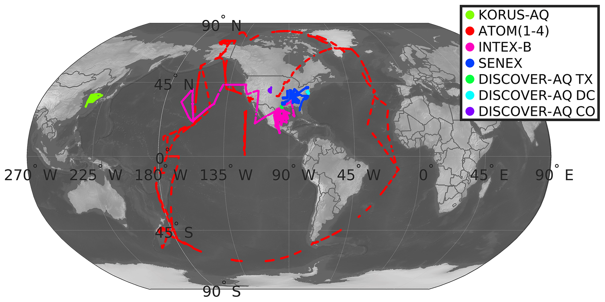
Figure 1 The locations of the seven different atmospheric composition aircraft campaigns used in this study. KORUS-AQ: Korea–United States Air Quality. ATom: Atmospheric Tomography Mission. INTEX-B: Intercontinental Chemical Transport Experiment – Phase B. SENEX: Southeast Nexus. DISCOVER-AQ refers to the Deriving Information on Surface Conditions from Column and Vertically Resolved Observations Relevant to Air Quality campaigns in Texas (TX), Washington DC (DC), and Colorado (CO).

For aircraft campaigns targeting polluted areas, including DISCOVER-AQ, KORUS-AQ, and SENEX, we use 10 s merged data, whereas for measurement campaigns conducted in relatively remote areas, such as INTEX-B and ATom, we use 30 s merged data. A more detailed description of the measurements is provided in Sect. 3.2. We exclude times with no measurements of NO, NO₂, or HCHO. The concentrations of OH and HO₂ were only measured during the INTEX-B, ATom, and KORUS-AQ campaigns. Likewise, we void any data points lacking either HO₂ or OH measurements for these campaigns. There are frequent gaps in some measurements, especially for VOCs, due to instrument issues or measurement techniques. Following Souri et al. (2020a), Miller and Brune (2022), Souri et al. (2023), and Bottorff et al. (2023), we fill the gaps in the measurements using a linear interpolation method, with no extrapolation allowed beyond 15 min. We drop any remaining gaps from the analysis. To better capture the rapid fluctuation in VOCs, we select the proton-transfer-reaction time-of-flight mass spectrometer (PTR-ToF-MS) instrument with high temporal resolution over the whole air sampler (WAS) when both instruments have measured the same quantity. Regarding the INTEX-B campaign, we drop the isoprene observations due to infrequent samples that downgrade the performance of our box model.

2.2 TROPOMI NO₂ and HCHO

We use recently reprocessed daily Level-2 (L2) TROPOMI tropospheric NO₂ and total HCHO columns (v2.4), derived from UV–Vis radiances captured by the European Space Agency (ESA) Sentinel-5 Precursor (S5P) spacecraft (∼ 328–496 nm) (Veefkind et al., 2012; De Smedt et al., 2021; van Geffen et al., 2022). This sensor has been operational since May 2018, providing global coverage of NO₂ and HCHO at ∼ 01:30 local standard time at the Equator. Since NO₂ and HCHO are optically thin absorbers in the UV–Vis range, meaning their concentrations do not substantially affect the sensitivity of the radiance to the optical thickness of the absorber, the retrieval follows a conventional two-step algorithm involving spectral fitting for slant column density (SCD) retrieval and air mass factor (AMF) calculations for conversion from SCDs to vertical column densities (VCDs). The product has a spatial resolution of 7.2 km (5.6 km as of August 2019) by 3.6 km at nadir. To remove unfit measurements, we use the provided quality flag (q_value) and choose only measurements above 0.75 for NO₂ and 0.5 for HCHO. As the L2 product is not provided on a regular grid, we use a mass-conserved regridding technique based on barycentric linear interpolation to map the data onto a 0.1° × 0.1° regular grid.

Van Geffen et al. (2022) demonstrated that the reprocessed TROPOMI tropospheric NO₂ columns exhibit a good level of correspondence with those obtained from ground-based MAX-DOAS (Multi-Axis Differential Optical Absorption Spectroscopy) sky spectrometers, with a correlation of 0.88 and a median bias of −23 %, improving on the older product versions, which were biased low by about 30 % with respect to ground-based measurements at polluted sites (Verhoelst et al., 2021). More information about the new modifications and their impacts on the retrieval can be found in van Geffen et al. (2022).

Studies by Vigouroux et al. (2020) and De Smedt et al. (2021) validated the reprocessed monthly-mean TROPOMI HCHO columns against Fourier-transform infrared (FTIR) and MAX-DOAS observations and found a good correlation above 0.8, with a negative bias of 20 %–30 % for polluted sites. The bias tends to be slightly positive or neutral over clean sites.

Error characterization of TROPOMI NO₂ and HCHO using ground-based retrievals

To propagate TROPOMI retrieval errors to the PO₃ product and to remove potential biases, we assume three origins for the errors: (i) random errors resulting from instrument noise, (ii) a fixed additive component that is magnitude-independent (i.e., a uniform offset persisting over all pixels), and (iii) unresolved systematic biases that are multiplicative and irreducible by oversampling. The first component is derived from the column precision variable provided along with the L2 product. In the spatial domain, we interpolate the squares of these errors in the same way we map the irregular L2 pixels onto the 0.1° × 0.1° regular grid. Moreover, we average the random errors over a month to reduce random noise by the square root of the number of pixels available at the same location (Eq. 3). Two other errors are determined by comparing FTIR observations for HCHO and MAX-DOAS observations for tropospheric NO₂ with TROPOMI data (Sect. 4.3.3). A detailed explanation of how these datasets are paired can be found in Vigouroux et al. (2020) and Verhoelst et al. (2021). Both datasets cover the period from 2018–2023.

To achieve an optimal linear fit ($y=ax+b+\mathit{\epsilon }$) between the paired observations – where a and b are the slope and offset to be determined, respectively – we follow a Monte Carlo chi-squared minimization such that ${\mathit{\chi }}^{\mathrm{2}}=\sum \frac{[y-f\left(x_i,a,b\right){]}^{\mathrm{2}}}{{\mathit{\sigma }}_y^{\mathrm{2}}+a^{\mathrm{2}}{\mathit{\sigma }}_x^{\mathrm{2}}}$ is minimized. In this equation, ${\mathit{\sigma }}_y^{\mathrm{2}}$ and ${\mathit{\sigma }}_x^{\mathrm{2}}$ are the variances of y (TROPOMI) and x (the benchmark, i.e., FTIR or MAX-DOAS), respectively; the subscript i refers to the ith observation point; and f is the proposed linear fit subject to optimization. In terms of TROPOMI NO₂ and HCHO, the errors are populated based on the L2 information. According to Verhoelst et al. (2021), a fixed error of 30 % is assumed for MAX-DOAS NO₂ observations whose values are above 1.4 × 10¹⁵ molec. cm⁻². Because of the detection limit of MAX-DOAS NO₂, we set errors for values below that threshold to 1.4 × 10¹⁵ molec. cm⁻². The FTIR retrieval errors described in Vigouroux et al. (2020) were used to populate the errors associated with this benchmark. The minimization is performed 10 000 times, each time with a set of random perturbations of x and y within their respective prescribed errors. This approach allows us to assess the robustness of the estimates across the range of errors associated with each data point.

The offset (a uniform additive term) and slope (a multiplicative error) drawn from the ground validation are used to correct the biases associated with TROPOMI via

$$\begin{array}{}\text{(1)}& {\mathrm{VCD}}_{\text{bias-corrected}}={\displaystyle \frac{{\mathrm{VCD}}_{\mathrm{original}}-\mathrm{offset}}{\mathrm{slope}}}.\end{array}$$

Since there are errors associated with this adjustment resulting from instrument and representation errors, we augment the error in the slope and offset with respect to the total error and label it as the constant error (e_const) using

$$\begin{array}{}\text{(2)}& e_{\mathrm{const}}^{\mathrm{2}}=e_{\mathrm{offset}}^{\mathrm{2}}+e_{\mathrm{slope}}^{\mathrm{2}}\times {\mathrm{VCD}}_{\text{bias-corrected}}^{\mathrm{2}},\end{array}$$

where $e_{\mathrm{offset}}^{\mathrm{2}}$ and $e_{\mathrm{slope}}^{\mathrm{2}}$ are the squares of the errors in the offset and slope, calculated from the linear regression (Eq. 1). Ultimately, the sum of all three errors constitutes the total error, as shown in the following:

$$\begin{array}{}\text{(3)}& e^{\mathrm{2}}=e_{\mathrm{const}}^{\mathrm{2}}+{\displaystyle \frac{\mathrm{1}}{m^{\mathrm{2}}}}\sum _{i=\mathrm{1}}^m{e}_{\mathrm{random},i}^{\mathrm{2}},\end{array}$$

where m is the number of samples for a given grid and time frame and $e_{\mathrm{random}}^{\mathrm{2}}$ represents the square of the random errors.

2.3 TROPOMI surface albedo

To account for the effect of surface albedo on photolysis rates (Sect. 2.5), we use a newly developed algorithm based on the directionally dependent Lambertian-equivalent reflectivity (DLER) UV surface albedo climatology derived from TROPOMI radiance (Tilstra et al., 2024). This new database leverages 60 months of TROPOMI reprocessed radiance data and is produced at a grid resolution of 0.125° × 0.125°. This product outperformed traditional Lambertian-equivalent reflectivity (LER) products, such as OMI, when they were compared to MODIS surface bidirectional reflectance distribution function (BRDF) results (Tilstra et al., 2024).

2.4 Modern-Era Retrospective analysis for Research and Applications, Version 2 – Global Modeling Initiative (MERRA-2 GMI)

To convert TROPOMI vertical column densities of HCHO and NO₂ to their volume mixing ratios in the PBL region, we use the MERRA-2 GMI (M2GMI) model (https://acd-ext.gsfc.nasa.gov/Projects/GEOSCCM/MERRA2GMI/, last access: 10 September 2023). This model serves as NASA's Goddard Earth Observing System (GEOS) chemistry–climate model (CCM), spanning the period of 1980–2019 and exploiting MERRA-2 (the second version of the Modern-Era Retrospective analysis for Research and Applications) to constrain meteorological fields (Orbe et al., 2017). The model uses the Global Modeling Initiative (GMI) chemical mechanism (Duncan et al., 2007), which involves over 120 species and 400 reactions. It has a resolution of approximately 0.5° latitude by 0.625° longitude, with 72 vertical layers stretching from the surface up to 0.1 hPa. Additional information about the configuration of this model can be found in Strode et al. (2019). To carry out the conversion, we apply the following conversion factor (γ) to the TROPOMI VCDs:

$$\begin{array}{}\text{(4)}& \mathit{\gamma }={\displaystyle \frac{{\stackrel{\mathrm{‾}}{q}}_{\mathrm{PBLH}}}{\frac{\mathrm{NA}}{g\times M_{\mathrm{air}}}\sum q\mathrm{dp}}},\end{array}$$

where ${\stackrel{\mathrm{‾}}{q}}_{\mathrm{PBLH}}$ is the average of the target trace gas mixing ratios within the planetary boundary layer height (PBLH), g is the acceleration of gravity (assumed to be 9.81 m s⁻²), NA is the Avogadro constant, M_air is the air molecular weight (assumed to be 28.96 g mol⁻¹), q is the target trace gas mixing ratio at a given altitude, and dp is the thickness of each vertical grid box in the model (simulated in hectopascals). The denominator in Eq. (4) represents the modeled VCD. We integrate the modeled partial VCDs up to the top of the atmosphere for HCHO and up to the tropopause pressure layer for NO₂.

2.5 The National Center for Atmospheric Research (NCAR) Tropospheric Ultraviolet and Visible (TUV) photolysis rate lookup table

To estimate the photolysis rates, JNO₂ (NO₂ + hν) and JO¹D (O₃ + hν), we use a comprehensive lookup table provided by the Framework for 0-D Atmospheric Modeling (F0AM) model (Sect. 3.2), created for clear-sky conditions. This lookup table is based on the calculation of more than 20 064 solar spectra over a wide range of solar zenith angles (SZAs) (a 0–90° range in steps of 5°), altitudes (a 0–15 km range in steps of 1 km), overhead total ozone column values (a 100–600 DU range in steps of 50 DU), and surface UV albedo values (a 0–1 range in steps of 0.2), using NCAR's Tropospheric Ultraviolet and Visible (TUV) radiation model (v5.2) and cross sections and quantum yields from the International Union of Pure and Applied Chemistry (IUPAC) and the Jet Propulsion Laboratory (JPL) (Wolfe et al., 2016). The L2 TROPOMI granule information populates the SZA, surface elevation, and surface UV albedo, while overhead total ozone columns are obtained from MERRA-2 GMI (Sect. 2.4), which is found to agree well with satellite observations (Souri et al., 2024). Any values between these tables are bilinearly interpolated for a smoother result.

3 Methods

In this section, we begin by discussing a robust regression model specifically developed for feature selection in the parameterization of PO₃. We then describe the training dataset created for this purpose. Following that, we introduce a clustering technique, utilized to organize the training data, which enables us to identify the key drivers of PO₃ variability. Finally, we provide a comprehensive overview of the PO₃ estimation algorithm by integrating data from the TROPOMI retrievals, ground-based remote sensing, and various models.

3.1 Least absolute shrinkage and selection operator (LASSO)

Through the use of multilinear regression models, it is possible to establish a simple but robust relationship between multiple variables and a target. However, when dealing with a large number of variables, there is a chance of introducing overfitting issues. This can lead to predictions that are either overly optimistic or unrealistic for values outside of the training dataset. To avoid this, it is recommended to simplify the model by removing variables that are loosely connected with the target or highly correlated with other variables. This process is known as “model shrinkage” and can narrow down the number of possible solutions (i.e., variance) at the cost of increasing the biases between the observed target and predictions. Ideally, we want a model that minimizes the sum of the bias and the variance. To achieve this, we can use the least absolute shrinkage and selection operator (LASSO) (Tibshirani, 1996). This operator considers the following regression:

$$\begin{array}{}\text{(5)}& Y=X\mathit{\beta }+\mathit{\alpha }+\mathit{\epsilon },\end{array}$$

where $Y=(y_{\mathrm{1}},\mathrm{\dots },y_n{)}^T$ is the response, X corresponds to n × p explanatory variables, $\mathit{\beta }=({\mathit{\beta }}_{\mathrm{1}},\mathrm{\dots },{\mathit{\beta }}_p{)}^T$ represents the coefficients, α is the intercept, and ε=(ε₁, …, ε_n)^T represents the noise variables. Moreover, n represents the number of data points, and p represents the number of explanatory variables. We can label the regression model as sparse when many of the β values are zero, and we can label it as high-dimensional when p≫n. LASSO attempts to select variables such that the following cost function is minimized:

$$\begin{array}{}\text{(6)}& \left(\widehat{\mathit{\alpha }}\widehat{\mathit{\beta }}\right)=\mathrm{argmin}\left\{{∥Y-X\mathit{\beta }-\mathit{\alpha }∥}_{\mathrm{2}}^{\mathrm{2}}+\mathit{\lambda }\sum _{i=\mathrm{1}}^p\left|{\mathit{\beta }}_i\right|\right\},\end{array}$$

where $\widehat{\mathit{\alpha }}$ and $\widehat{\mathit{\beta }}$ represent the optimized intercept and coefficients, respectively; λ is a non-negative regularization factor subject to tuning; i is the subscript of the ith explanatory variable; and ∥.∥₂ is the L2-norm-based operator. The first term on the right side of Eq. (6) minimizes the squares of the residuals, whereas the second term reduces the sum of the absolute values of the coefficients, resulting in a simpler model with fewer parameters. Without the second term, the regression model becomes an ordinary least-squares estimation. The most critical element here is λ. A large λ value results in more aggressive regularization, leading to more model shrinkage, whereas a small value preserves a high-dimensional model. To optimize this value, we discretize λ into 100 values between 10⁻⁴ and 10¹, divide the training dataset into 10 folds (i.e., split the dataset into equally sized segments), determine the average of the cross-validated error prediction among all folds, and find the λ value that yields the smallest error. The final solution ensures a balanced model with respect to model parsimony and bias. All explanatory variables are standardized during the regularization procedure such that their mean becomes zero and their standard deviation becomes 1.

3.2 Photochemical box modeling

To produce training datasets for LASSO-based PO₃ estimation, we use the Framework for 0-D Atmospheric Modeling (F0AM) box model (v4; Wolfe et al., 2016), constrained by a wide range of observations. These observations ensure that the model achieves a realistic range of values consistent with those found in the atmosphere. We follow past setups that apply the Carbon Bond 6 (CB06, r2) chemical mechanism within the F0AM model (Souri et al., 2020a, 2023). The model is constrained by aircraft data, including meteorology, photolysis rates, and trace gas concentrations. The model configuration and observations used are listed in Table S2.

Once the model is initialized and held constant with respect to a wide range of constraining quantities, it runs with a 30 min integration time cycle for 5 d to approach a steady-state environment. Several key compounds, including OH, HO₂, HCHO, polyacrylonitrile (PAN), NO, and NO₂, are initialized with aircraft observations, but they are left free to cycle with incoming solar-radiation variability. These compounds play a crucial role in validating the efficacy of model performance as well as the adequacy of the observations used as constraints. In particular, allowing HCHO to vary freely enables us to assess whether our mechanism for VOC treatment, the steady-state conditions, and the number of measured VOCs are sufficient for reasonably reproducing its concentrations. Although the individual concentrations of NO₂ and NO are not constrained, we constrain the total NO_x (NO + NO₂). Not all aircraft campaigns measured all photolysis rates included in the chemical mechanism. We first initialize the photolysis rates included in CB06 using the lookup tables described in Sect. 2.5. If any photolysis reaction rates in CB06 were measured, we replace the initial guess with the observed values. For reactions with unmeasured photolysis rates, we apply a scaling factor made from the average ratio of the observed J values to the modeled J values. This approach is a sensible choice for accounting for large particles, such as clouds, as their extinction coefficient is somewhat non-selective in the UV–Vis range; however, applying a wavelength-independent scaling factor may introduce some biases into optically complex environments introduced by aerosols.

It is essential to acknowledge the inherent limitations of the box model in our research. The model does not consider the diverse physical loss pathways that trace gases may undergo, including deposition and transport. As a result, we simplify the physical loss by employing a first-order dilution rate equivalent to a lifetime of 24 h. This approach ensures that unconstrained trace gases, which take longer to break down, do not accumulate over time. Exact knowledge of dilution factors requires understanding molecular and turbulent diffusion, entrainment, detrainment, and deposition rates, all of which are unknown at the microscale level of aircraft observations. Nonetheless, studies by Brune et al. (2022) and Souri et al. (2023) showed that HO₂, OH, NO_x, and HCHO are relatively immune to the choice of dilution factor, whereas RO₂ mixing ratios can vary, introducing some biases into PO₃ estimates.

We determine the simulated PO₃ using

$$\begin{array}{}\text{(7)}& {\mathrm{PO}}_{\mathrm{3}}={\mathrm{FO}}_{\mathrm{3}}-{\mathrm{LO}}_{\mathrm{3}},\end{array}$$

where LO₃ represents all possible chemical loss pathways of ozone (a negative stoichiometric multiplier matrix) and FO₃ represents all possible chemical pathways producing ozone molecules (a positive stoichiometric multiplier matrix). This calculation is theoretically equivalent to the value obtained from a chemical solver quantifying the number of ozone molecules produced/lost at each model time step. The adoption of Eq. 7 facilitates the direct comparison of PO₃ estimations with estimations derived from other models, including chemical-transport-model-based results (see Fig. 10 in Souri et al., 2021). Furthermore, it allows for seamless integration of these estimates into Lagrangian transport models for ozone forecasting purposes.

3.3 Clustering

The aim of using a classifier to categorize the large quantity and variety of aircraft data into groups with similar features is to enable us to study the primary contributors to PO₃ under different chemical, solar, and meteorological conditions. Additionally, this approach helps us understand the range of atmospheric conditions included in the training dataset. To accomplish this, we employ a widely used technique known as k-means, which has been used in a variety of applications (e.g., Beddows et al., 2009; Souri et al., 2016b; Govender and Sivakumar, 2020). In this approach, centroids are distributed randomly throughout a multidimensional dataset, with each centroid representing a distinct class. The algorithm then assigns a label to each data point by identifying its shortest Euclidean distance to the centroids. Following the labeling of all data points, the algorithm updates the centroids based on the means of the newly labeled groups. This process continues iteratively until there is minimal change in the location of the centroids. It is worth noting that k-means does not guarantee an optimal solution, so we reinitialize the classification 1000 times with a new set of initial centroids. We select the result with the lowest value for the sum of the Euclidean distances among the data points and centroids to ensure the outcomes are not influenced by random seeding.

Redundant features in the input can significantly compromise the effectiveness of the classification, so we apply principal component analysis (PCA) to a matrix of datasets (Z) with n data points and p features to reduce the dimensions to those of a PCA-transformed matrix (Z^′), i.e., n × q, where q < p. Despite this reduction in dimensions, Z^′ preserves a significant variance in Z, helping us to overcome issues of dimensionality or overfitting.

We select 11 features simulated by the F0AM model, many of which are set to the observed values or have observationally constrained precursors. These features comprise the SZA, HCHO $/$ NO₂, HCHO × NO₂, HCHO, NO₂, pressure, temperature, jNO₂, jO¹D, H₂O, and NO₂ $/$ NO_y (NO_y = NO + NO₂ + PAN + HNO₃ + alkyl nitrate + N₂O₅). There are indeed correlations among these features, such as between the SZA and jNO₂ or between HCHO and HCHO × NO₂; nonetheless, we use PCA to eliminate the possibility of these correlated factors causing overfitting issues.

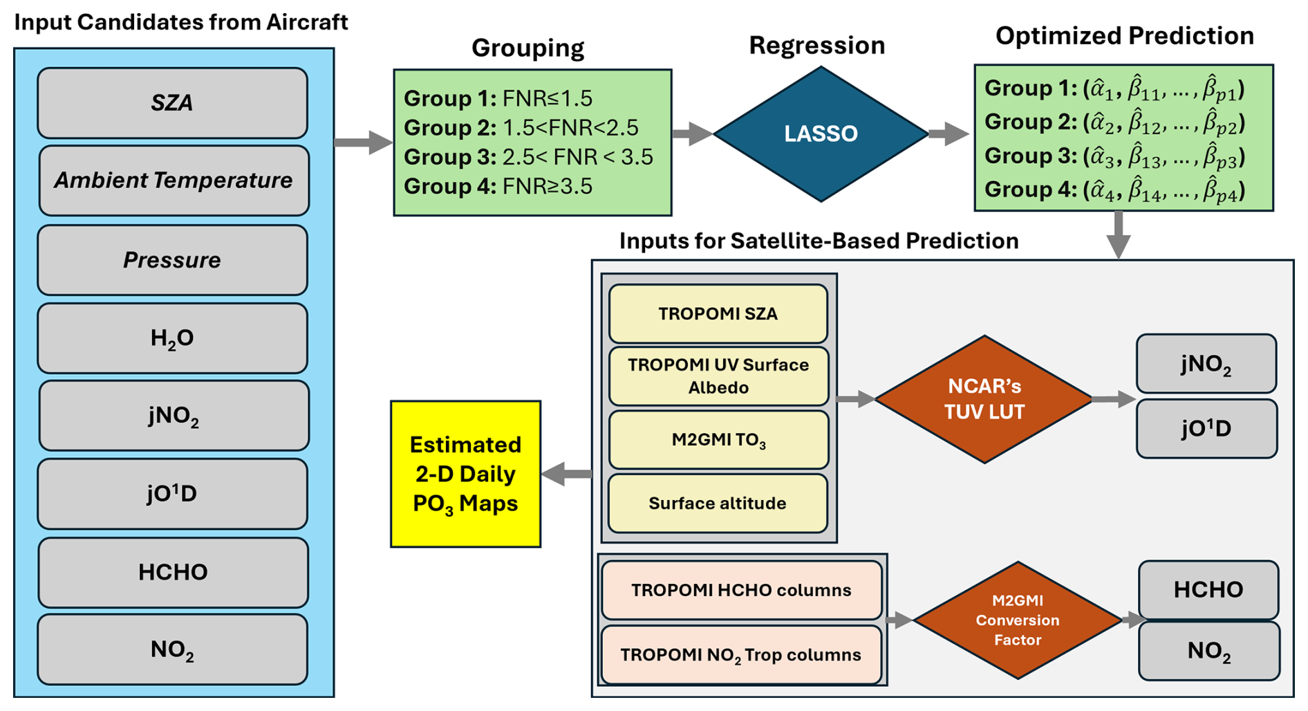
Figure 2 Schematic illustration of the daily PO₃ estimation process demonstrated in this study. This process consists of two major steps: (1) formulating PO₃ as a function of various prognostic inputs derived from the box model results and (2) predicting PO₃ based on optimized features/coefficients suggested by LASSO and using information obtained from TROPOMI, the TUV model, and M2GMI. LUT: lookup table. Trop columns: tropospheric columns.

3.4 The estimation of PO₃

In order to predict PO₃, we developed empirical equations using LASSO to link PO₃ with various relevant prognostic candidates related to ozone chemistry. A schematic presentation of how this estimation can be carried out to provide daily PO₃ maps corresponding to the TROPOMI revisit time across the globe is shown in Fig. 2. It is important to note that relying solely on linear regressions for a non-linear problem is not a viable approach. To address this, we divided the data points into four distinct groups based on FNR values, meaning we divided a non-linear realm into smaller linear segments (i.e., an empirical linearization). In a study by Souri et al. (2023), a wide range of aircraft observations and box model results were used to determine that FNR values of ∼ 1.7 were a universal threshold for separating NO_x-sensitive from VOC-sensitive regimes. We found that by breaking down the data points into slightly weaker or stronger variations within the regimes, we can improve the accuracy of our results. As a result, we established four distinct groups: VOC-sensitive regimes (FNR < 1.5), transitional regimes (1.5 < FNR < 2.5 and 2.5 < FNR < 3.5), and NO_x-sensitive regimes (FNR > 3.5). The coefficients and intercepts based on the LASSO regressions for each group were computed separately. From a long list of explanatory parameters, we selected the SZA, temperature, pressure, H₂O, jNO₂, jO¹D, HCHO, and NO₂ as the most sensible candidates. The reasoning behind this selection will be discussed in Sect. 4.2.

Once the LASSO parameters are determined, we apply the linear functions to the variables modeled/observed in the PBL region. We show that the LASSO method suggests dropping the SZA, temperature, water vapor, and pressure as they do not provide significant information on PO₃ compared to the other parameters. As for jNO₂ and jO¹D, we use the NCAR's TUV lookup table, described in Sect. 2.5. HCHO and NO₂ are derived by converting the bias-corrected TROPOMI VCDs into PBL mixing ratios using MERRA-2 GMI, as described in Sect. 2.4. To carry out this conversion, we multiply the satellite VCDs by the ratio of the averaged modeled mixing ratios of a target gas (i.e., NO₂ or HCHO) in the PBL region, divided by the modeled VCDs (Sect. 2.4). The PBL field also comes from MERRA-2 GMI.

4 Results and discussion

4.1 Box model validation

In order to assess the accuracy of the assumptions used in the box model's setup, which involves factors such as chemical mechanisms, dilution rates, and photolysis rate corrections, we will compare the simulated values of HCHO, NO₂, NO, PAN, HO₂, and OH with their actual measured values. This comparison will help us determine whether our model falls within an acceptable range of errors, as seen in other reputable studies of photochemical box modeling. This comparison is shown in Fig. 3, which displays scatterplots illustrating data collected from all seven aircraft campaigns. A discussion of each parameter follows:

• HCHO. The box model is proficient in capturing over 77 % of the variance in observations with less than 15 % absolute bias. While many box modeling studies prefer to have this compound constrained to potentially enhance the representation of HO_x, doing so comes with the trade-off of hindering our ability to validate the number and quality of observed HCHO precursors and/or the treatment of VOCs. Besides the study by Souri et al. (2023), the work of Marvin et al. (2017) serves as one of the few studies that did not constrain this compound, aiming to verify the efficacy of different pathways involved in HCHO formation and loss as simulated by various chemical mechanisms. Marvin et al. (2017) reproduced HCHO formation during the SENEX campaign using the CB06 mechanism, achieving an R² value of 0.66 and a bias of 32 % with 1 min averaged samples. In comparison, we recreated a variance of 86 % in observed HCHO during the same campaign, with a bias of 23 % (Fig. S1), using 10 s averaged samples. The remaining unresolved variance can be attributed to an incomplete list of VOC measurements from several campaigns, including DISCOVER-AQ, and errors in VOC measurements. It is unlikely that the chemical mechanism is the reason for this, as Marvin et al. (2017) did not observe substantial differences in R² values among various chemical mechanisms, including the near-explicit Master Chemical Mechanism (MCM). A mild underestimation of HCHO could likely be due to the steady-state assumption, a fixed arbitrary dilution factor, or uncertain isoprene chemistry (Archibald et al., 2010; Wolfe et al., 2016; Marvin et al., 2017).

• NO₂ and NO. Comparisons for both species demonstrate a high degree of correspondence for values above 0.1 ppbv. Nonetheless, we note a substantial amount of fluctuation in the simulations in clean regions, particularly for NO. While we cannot rule out the possibility of chemical-mechanism uncertainty contributing to this deviation, the reported measurement errors for NO₂ and NO are usually ±0.05 and ±0.1 ppbv, respectively. Consequently, it is likely that the measurement errors resulted in more spread in the comparisons. In particular, Shah et al. (2023) found that these measurements could be contaminated by various reactive nitrogen species in remote regions, precluding a robust validation of atmospheric models.

• PAN. Our model reproduced 61 % of the variance observed in PAN with marginal absolute bias. According to Xu et al. (2021), the presence of oxygenated VOCs, particularly acetaldehyde, and the NO $/$ NO₂ ratio are key factors controlling PAN levels. Although we constrained acetaldehyde, variations in the NO $/$ NO₂ ratio in heavily polluted regions (where NO_x levels exceed 1 ppbv) may have potentially led to biases in PAN simulations. Furthermore, our model's dilution factor was arbitrarily set, and it is possible that any bias caused by this factor was canceled out by other effects, leading to seemingly bias-free performance. However, Souri et al. (2023) showed that an incorrect dilution factor can significantly impact PAN performance, causing a sharp decline in R², resulting in a value below 30 %. Therefore, the fact that our box model performed well with respect to PAN could be an indication that our choice of dilution factor was reasonable.

• HO₂ and OH. Based on our analysis of HO₂ and OH simulations during the KORUS-AQ, INTEX-B, and ATom campaigns, we found a reasonable level of correspondence (R² > 0.6) with the performance observed in previous studies conducted by Souri et al. (2020a), Brune et al. (2022), Miller and Brune (2022), and Souri et al. (2023), which focused on some of these campaigns. Although the box model OH simulations reported in Brune et al. (2020) regarding the ATom campaign seemed to be better than ours (an R² value of ∼ 0.8 vs. an R² value of ∼ 0.6), it is important to consider that their observations were averaged over 1 min intervals as opposed to 30 s intervals, as seen in our study. It should also be noted that there can be large errors in ATHOS (Airborne Tropospheric Hydrogen Oxides Sensor) HO_x measurements, reaching up to ±40 % (Miller and Brune, 2022), so recreating the exact variance in the observations should not be the main objective. Nonetheless, the performance of our simulations in terms of HO_x compared to observations suggests that the number of measured compounds and chemical mechanisms used in the model was effective. Our model's performance with respect to HO_x is comparable to that of more sophisticated mechanisms that encompass a larger number of measured species (Brune et al., 2022; Miller and Brune, 2022).

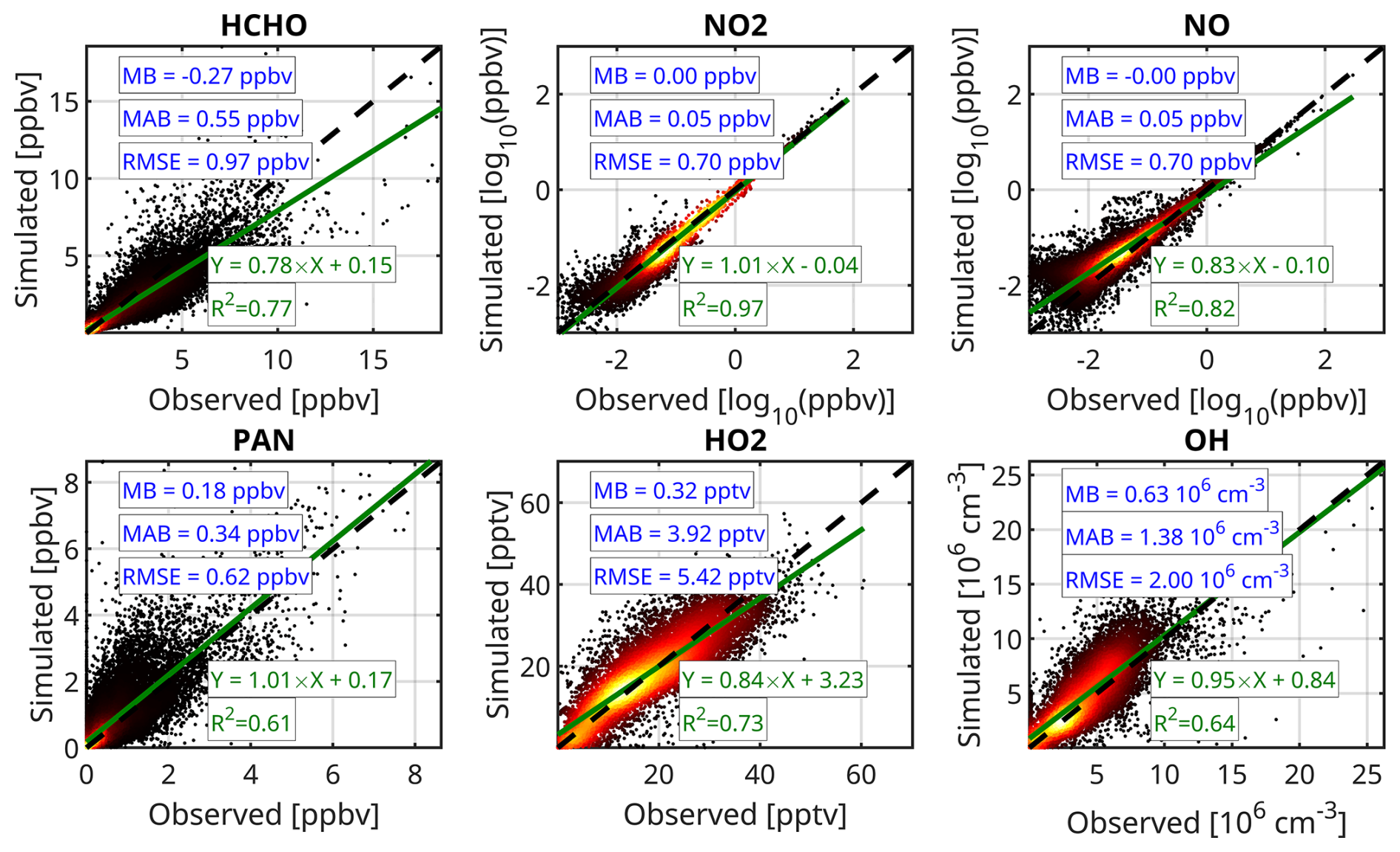
Figure 3 A scatterplot comparison of simulations with observed concentrations for six unconstrained species. More than ∼ 133 000 observations were used for HCHO, NO₂, NO, and PAN. HO_x data points were limited to ∼ 55 000 observations. Heat maps show the density of the data. Linear fits were calculated using the ordinary least-squares method. MB: mean bias. MAB: mean absolute bias.

Overall, while there are inevitably some differences between the box model results and observations, they are consistent with what other studies have found in similar aircraft campaigns. Our extensive box model results, which consider a variety of meteorological, chemical, and photolysis rates, demonstrate satisfactory results for unconstrained compounds across a wide range of atmospheric conditions. This suggests that our training dataset, derived from the box model, is a reliable source for understanding local PO₃.

It is important to note that even if a simulated data point does not match up perfectly with actual observations, it still plays a role in establishing PO₃ and other explanatory variables. Hypothetically, one can generate synthetic training data points by running the box model with random numbers for the inputs; however, only a fraction of these can be truly observed in nature. Therefore, a mild outlier in our training dataset should be viewed as less likely to occur in nature (presuming that these campaigns represent all conditions occurring in nature) but still as a valuable data point derived from a physical model that can help bridge PO₃ with explanatory variables.

4.2 Classification of aircraft data

Following the method described in Sect. 3.3, we cluster the cloud of aircraft data (∼ 133 000 points) into seven distinct classes. We describe these classes using three categories: pollution level, altitude, and SZA magnitude. Figure 4 illustrates violin plots of these classes for various chemical, solar, and meteorological conditions. Figure 5 presents corresponding violin plots of simulated PO₃. A discussion of each class and its relationship to PO₃ follows:

• Class 1 (C1) – clean, high-altitude, high-SZA conditions. Characterized by high-altitude flights, cold ambient temperatures, and a negligible water vapor content, this class consists of observations typically taken at a relatively high SZA, with a median value of 50°. While high-altitude observations under clear-sky conditions often exhibit high photolysis rates due to reduced overhead ozone, the relatively high SZA of this class leads to low photolysis rates. FNRs tend to be large in this class due to a higher amount of HCHO relative to NO₂, while FNP (HCHO × NO₂) values and NO₂ $/$ NO_y ratios are low due to the pristine conditions. The lack of sufficient ozone precursors and reduced photochemistry make this class undergo the lowest PO₃ rates, with a median of 0.11 ppbv h⁻¹.

• Class 2 (C2) – clean, high-altitude, low-SZA conditions. This category represents samples collected under low-SZA conditions, resulting in the highest photolysis rates among all classes. The mass of the ozone precursors and the ozone sensitivity conditions are similar to those in C1. However, C2 PO₃ rates are approximately 60 % higher than those in C1 due to increased photochemistry.

• Class 3 (C3) – moderately clean, medium-altitude, high-SZA conditions. This class is characterized by observations collected at medium altitudes and a high SZA. Airsheds in C3 experienced more polluted air compared to those in C1 and C2 due to their proximity to the surface. Photolysis rates in C3 are lower than those in C1, possibly due to higher levels of overhead ozone, although we cannot rule out the influence of varying surface albedo between the classes. Despite the lower photolysis rates, C3 PO₃ levels (0.28 ppbv h⁻¹) are higher than those of C2 and C1, indicating that pollution levels can have a more significant impact than favorable conditions for photochemistry.

• Class 4 (C4) – moderately clean, medium-altitude, low-SZA conditions. This class differs from C3 in having a lower SZA (resulting in more photochemistry) and a slightly smaller number of ozone precursors. As a result of the lower ozone precursor concentration, C4 PO₃ levels (0.19 ppbv h⁻¹) are not only lower than those in C3 but also comparable to those in C2. This again implies that the concentration of ozone precursors is more important than photochemistry under these conditions.

• Class 5 (C5) – extremely polluted, low-altitude, low-SZA conditions. This class features the highest concentration of ozone precursors among all classes (median FNP value of ∼ 58 ppbv²). Furthermore, it is characterized by low photolysis rates, due to its proximity to the surface, and high NO₂ $/$ NO_y ratios, indicative of a localized polluted airshed. Compared to the aforementioned classes, this class has the lowest FNR, indicating that it is mainly located in the VOC-sensitive regime. C5 PO₃ values are much higher than those in the aforementioned classes, reaching 3.0 ppbv h⁻¹.

• Class 6 (C6) – polluted, low-altitude, low-SZA conditions. While this class shares similar features with C5 in terms of altitude, photolysis rates, and meteorology, it has a lower value (with a median value of 8 ppbv²). Despite the lower FNP value, C6 exhibits the highest levels of PO₃ (5.2 ppbv h⁻¹) among all classes. This is a result of reduced non-linearities as this class does not often fall into an extreme VOC-sensitive regime (with a median FNR of ∼ 1.0), where nitrogen oxides (NO_x) can hamper ozone production. This tendency aligns with the findings of Souri et al. (2023), who also found that the highest amount of PO₃, lying between the transitional regimes, gravitated toward the VOC-sensitive regime due to abundant ozone precursors and reduced negative chemical feedback from NO_x.

• Class 7 (C7) – moderately polluted, low-altitude, low-SZA conditions. C7 is characterized by aged air close to the surface and slightly higher photolysis rates compared to those in C5 and C6. C7 PO₃ levels amount to 2.5 ppbv h⁻¹, only slightly lower than the C5 value, despite having a much lower FNP value (with a median of 0.9 ppbv²). This could be due to the combined effect of higher photolysis rates and reduced non-linear ozone chemistry.

Figure 4 Violin plots illustrating six different parameters derived from the box model, clustered into seven distinct categories. Each cluster is described using three types of labels: one for air pollution levels (C (clean), M (moderately clean), P (moderately polluted), P+ (polluted), and P++ (extremely polluted)), one for altitude (H (high), M (medium), and L (low)), and one for the SZA (H (high) and L (low)). Each white dot represents the median, and the bars indicate the 75th and 25th percentiles. Both the FNRs and FNPs are scaled using a logarithmic function to enable the simultaneous visualization of both low and high values within a single plot.

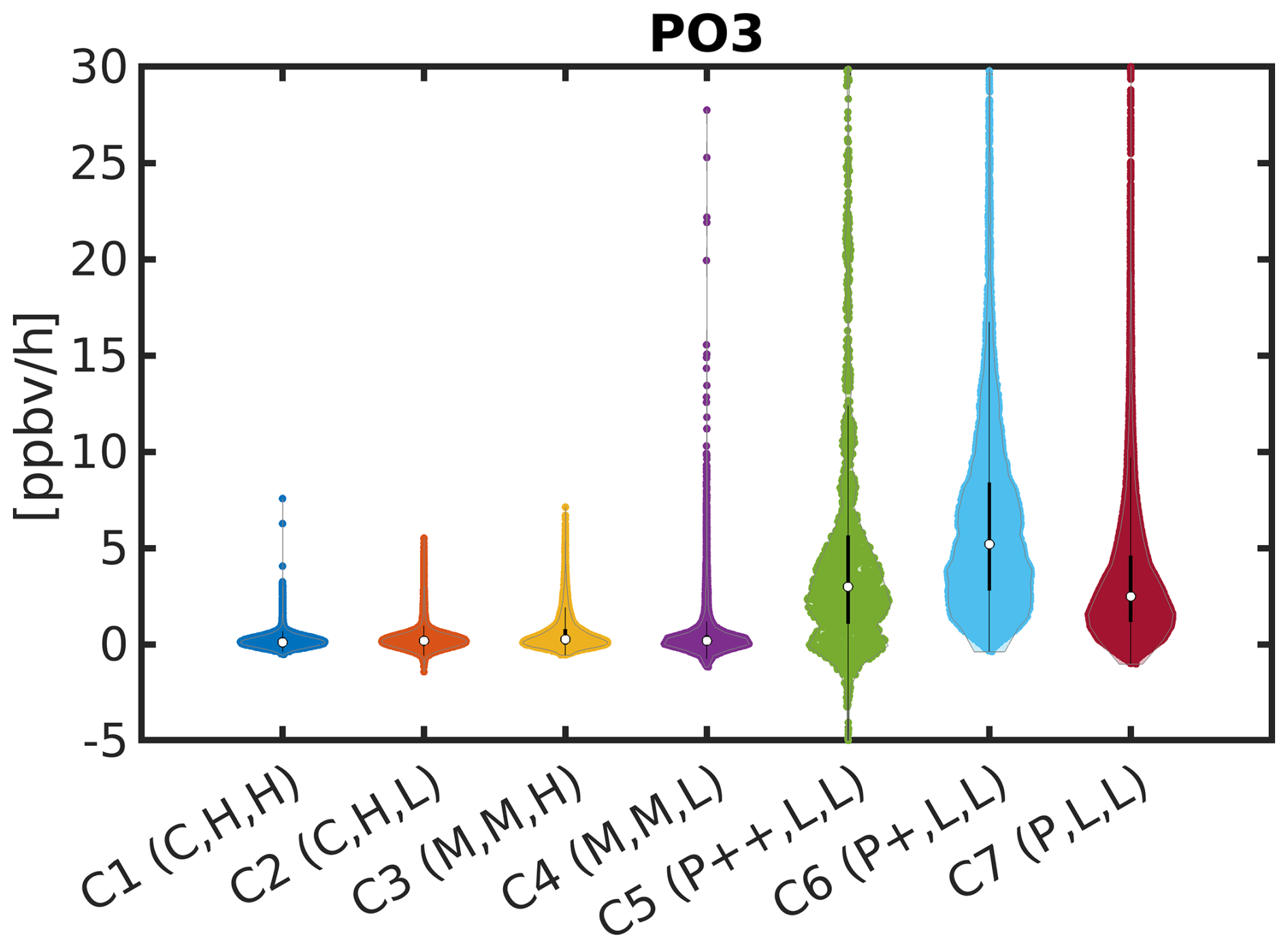
Figure 5 Violin plots of simulated PO₃ corresponding to the seven clusters described in Fig. 4. The lowest PO₃ levels are seen in remote regions (air pollution levels: C–M), where ozone precursors are minimal. The highest PO₃ levels do not occur in the most polluted (P++) regions due to the non-linear ozone chemistry.

An analysis of the aircraft data revealed that the levels of HCHO and NO₂, as well as the rates of jNO₂ and jO¹D photolysis, play an important role in influencing PO₃. Additionally, the FNR can offer insights into the sensitivity of PO₃ to its main precursors. These findings align with numerous studies that have examined the factors driving PO₃ (e.g., Duncan and Chameides, 1998; Thornton et al., 2002; Kleiman et al., 2002; Gerasopoulos et al., 2006; Chatfield et al., 2010; Baylon et al., 2018; Wang et al., 2020; Souri et al., 2023). Consequently, our PO₃ estimates incorporate HCHO, NO₂, jNO₂, jO¹D, and FNRs. While the cluster analysis did not definitively indicate whether meteorological conditions impact PO₃, we also include ambient temperature, water vapor, pressure, and the SZA to determine whether they provide any additional insights into PO₃ estimates.

4.3 Estimates of PO₃

4.3.1 LASSO coefficients

Armed with a procedure that identifies important features in a linear model (Sect. 3.1), we now explore the use of LASSO for PO₃ estimation. We make use of all data points generated by the observationally constrained box model across various atmospheric composition campaigns. Regarding the selected variables shown in Fig. 2, the LASSO algorithm assigns zero coefficients to the SZA, pressure, temperature, and water vapor, indicating that they offer less valuable information compared to the other variables. This decision was made by systematically adjusting the regularization factor within a 10-fold cross-validation framework to identify the optimal factor that balances solution variance and prediction bias. As a result, the LASSO algorithm suggests that HCHO, NO₂, jNO₂, and jO¹D contain sufficient information to accurately predict PO₃ for the most part.

Table 1 Calibrated coefficients derived from the LASSO estimator using seven atmospheric composition aircraft campaigns.

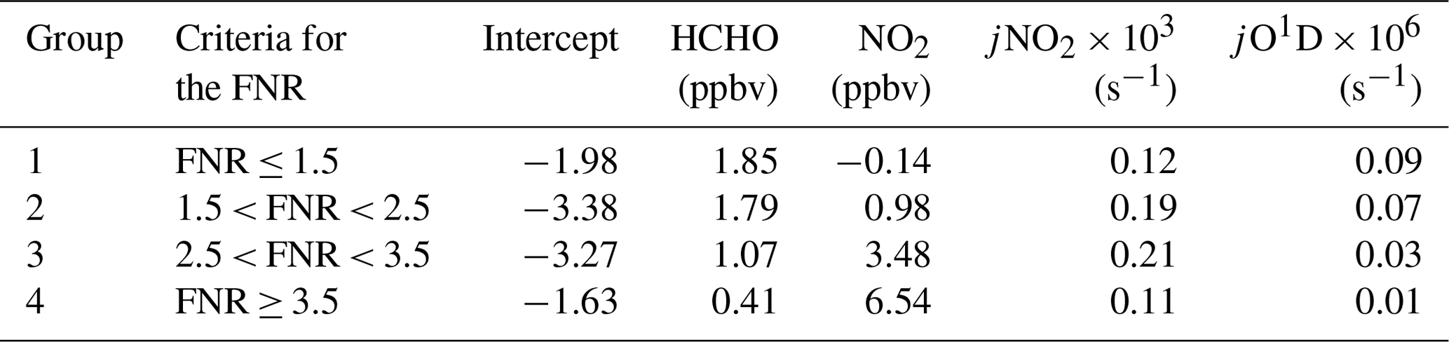
Table 1 provides the intercepts and corresponding coefficients for four different regions, classified by FNRs. While we do not expect a statistical model to fully single out the cause-and-effect relationship between explanatory variables and the target, we note that it exhibits a basic understanding of ozone chemistry; specifically, the HCHO coefficients increase as the FNR decreases (i.e., in more VOC-sensitive conditions). The same tendency is evident with respect to NO₂ and higher FNRs (i.e., more NO_x-sensitive conditions). The negative coefficient of NO₂ in regions where FNR values ≤ 1.5 implies some level of non-linear feedback embedded in this parameterization. Both jNO₂ and JO¹D have positive coefficients across all chemical conditions, suggesting that higher photolysis rates accelerate PO₃. JO¹D has a smaller effect than jNO₂ on PO₃ over remote regions (with FNR values ≥ 3.5), perhaps due to redundant information compared to that concerning jNO₂.

4.3.2 Validation of PO₃ predictions

The validation of PO₃ predictions against the box model results is performed in three progressively stringent stages: (i) using all data points included in the LASSO algorithm, (ii) randomly dropping data points, and (iii) dropping each air quality campaign from the LASSO estimation and using its data as a benchmark.

Figure 6a shows the scatterplot of predicted PO₃ against the box model for all data points used to estimate the coefficients described in Sect. 4.3.1. Despite the algorithm's simplicity, we can recreate more than 88 % of the variance in PO₃ with negligible absolute bias. Importantly, this suggests that our scientific problem is not overly complex. There is less than 30 % bias relative to the mean absolute bias of the prediction. The positive offset and slope smaller than 1 indicate a mild underestimation (overestimation) of PO₃ in polluted (clean) regions. Figure 6b shows the same analysis for 20 000 randomly chosen data points (∼ 15 % of the total), which we purposefully dropped from the LASSO estimation to assess whether the predictor model can replicate values for points not used during the training. We find almost identical statistics for these points, suggesting that the prediction stays robust for points outside the training dataset. However, the most stringent method involves dropping each campaign dataset entirely to understand where the prediction model struggles most.

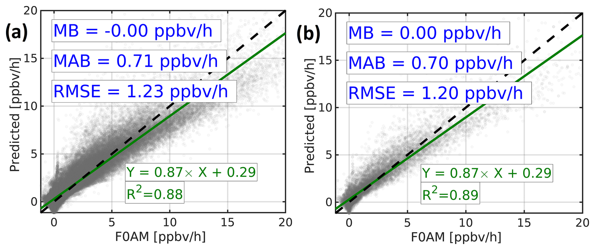
Figure 6 Scatterplots comparing observationally constrained F0AM model PO₃ with predictions based on proposed algorithms for either (a) all data points or (b) 20 000 data points randomly dropped as benchmarks. Despite the simplicity of the algorithm, we can reproduce a large variance in PO₃ using only four explanatory variables.

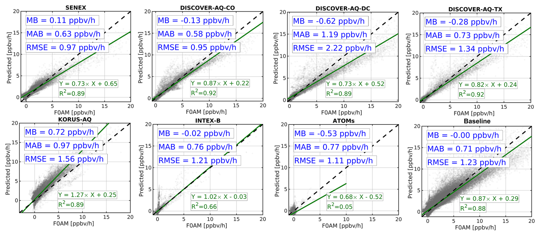
Figure 7 As in Fig. 6b but with each campaign dropped from the LASSO estimation and subsequently used as an independent benchmark. The designed algorithm demonstrates a high degree of skill in predicting PO₃ in polluted regions; however, it performs poorly in pristine areas.

Figure 7 shows several subplots pertaining to campaigns dropped from the analysis. It is immediately evident that our PO₃ estimation demonstrates considerable skill in capturing PO₃ in most polluted cases, including those from DISCOVER-AQ, KORUS-AQ, and SENEX, without using their individual datasets. This provides convincing evidence of a high degree of generalizability for the predictor. However, the model shows reduced performance with respect to INTEX-B for PO₃ values < 1 ppbv h⁻¹. Moreover, the model's predictive power is consistently poor for ATom, where a significant fraction of airsheds were sampled in pristine areas. We observe similarly poor performance for PO₃ values < 1 ppbv h⁻¹ in other campaigns, such as KORUS-AQ. Therefore, it is difficult to have confidence in the model's predictive power in remote regions, which may be due to the lack of inclusion of HO_x, halogens, and H₂O in the fit, as these can serve as important sinks for tropospheric ozone in those areas (Simpson et al., 2015). Nonetheless, while our predictive accuracy remains poor for this specific subset of data, the practical utility and significance of these specific regions (i.e., pristine areas) for air quality applications are notably limited. Given these results, we limit our predictions to PO₃ values > 1 ppbv h⁻¹ for the subsequent analyses.

4.3.3 TROPOMI NO₂ and HCHO validation

To build confidence in our quantitative application of TROPOMI data for PO₃ estimates, we validate the daily tropospheric NO₂ and total HCHO columns against MAX-DOAS and FTIR observations based upon the validation framework outlined in Vigouroux et al. (2020) and Verhoelst et al. (2021). Both paired datasets were expanded to cover late 2023, providing a fuller picture of TROPOMI error characterization compared to previous studies. Figure 8 presents a comparison of daily TROPOMI data, the benchmarks, and the optimal fit associated with their errors for the period 2018–2023.

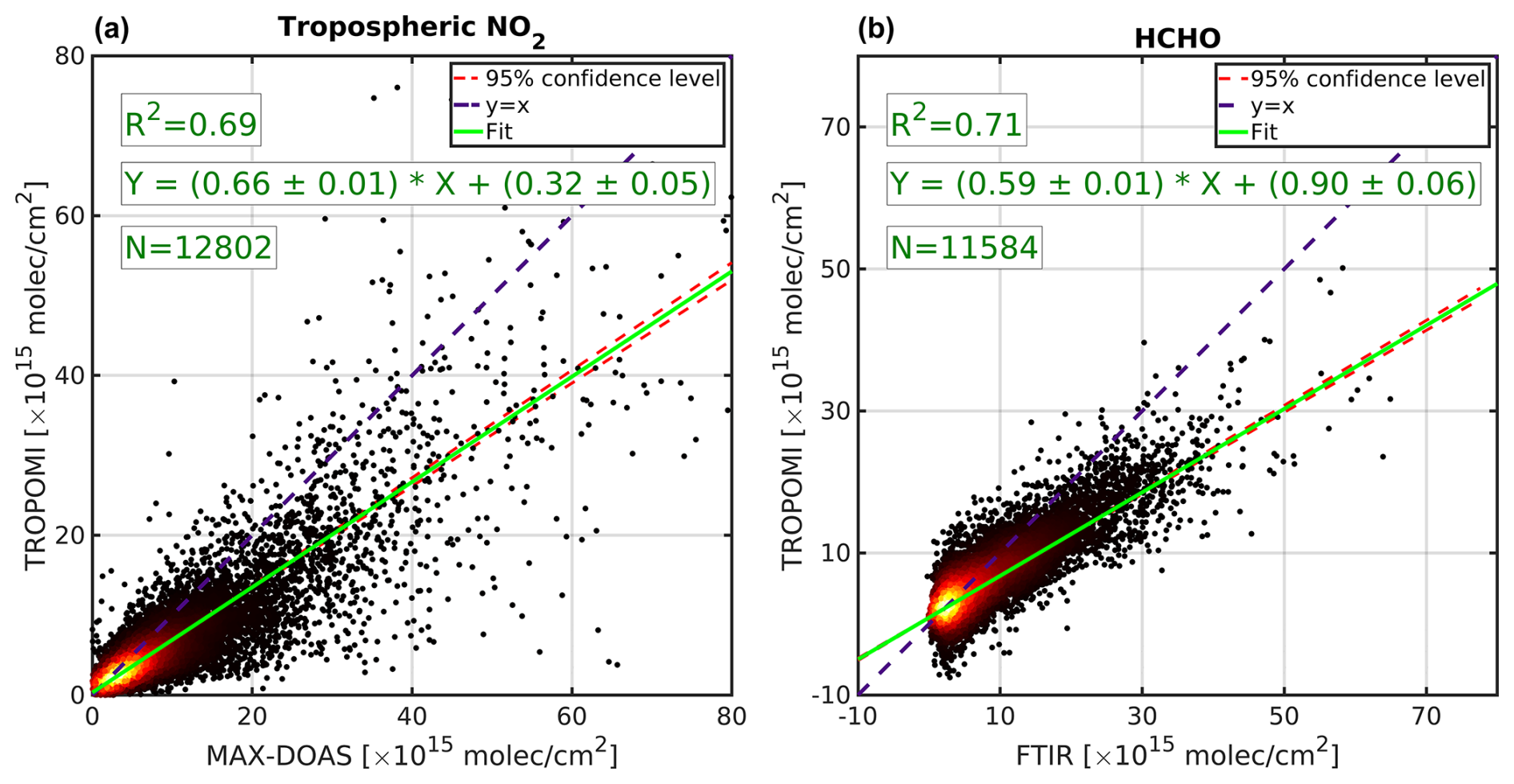
Figure 8 Comparisons of TROPOMI tropospheric NO₂ with MAX-DOAS observations (a) and TROPOMI HCHO with FTIR observations (b). The data points cover the period from 2018–2023. Errors in both ground-based remote sensing measurements and TROPOMI are considered in the fit. The data curation procedure is discussed in Verhoelst et al. (2021) and Vigouroux et al. (2020). A slope smaller than 1 suggests that both HCHO and NO₂ retrievals are underestimated in polluted regions.

In the context of tropospheric NO₂ comparison, we observe a slope smaller than 1 (∼ 0.66) with a positive offset (0.32 × 10¹⁵ molec. cm⁻²). This tendency has been repeatedly documented in various studies for different satellites or benchmarks (e.g., Griffin et al., 2019; Choi et al., 2020; Verhoelst et al., 2021; van Geffen et al., 2022). A slope smaller than 1, originating from unresolved systematic biases, implies that TROPOMI is biased low in polluted regions. A slightly positive offset suggests that TROPOMI NO₂ is biased high in remote regions. The errors in the slope and offset are relatively small, providing evidence of the robustness of the optimal fit against the dataset variance. Nonetheless, we incorporate them into Eqs. (2) and (3) to take the adjustment error into consideration.

Despite the inherent difficulty in obtaining HCHO observations from UV–Vis imagery (Gonzalez Abad et al., 2019), the HCHO comparison exhibits good alignment with the benchmarks. As in the previous comparison, the slope is smaller than 1 (∼ 0.59), and the offset is positive (∼ 0.9 × 10¹⁵ molec. cm⁻²), agreeing within 10 % of studies by Vigouroux et al. (2020) and De Smedt et al. (2021). Consequently, we consider the fit errors and adjust all VCDs based on the slope and offset obtained from this comparison.

4.3.4 Maps of PO₃ across various regions with qualitative descriptions

Taking advantage of the wealth of bias-corrected TROPOMI observations, we present the first-ever reported maps of PO₃ at a 0.1 × 0.1° resolution within the PBL for July 2019 across various geographic regions. Moreover, due to the explicit nature of our algorithm, it is straightforward to break down the contributors of PO₃ to gain insights into how each driver has shaped the distribution of PO₃. Therefore, in addition to PO₃ maps, we will show the magnitudes of various drivers of PO₃, including NO₂, HCHO, and FNR concentrations in the PBL region and the sum of scaled jO¹D and jNO₂ values, as well as their contributions to PO₃. It is worth noting that these maps are only a snapshot of PO₃ as its precursors can exhibit large interannual and interdecadal variability caused by meteorology, chemistry, and emissions. A discussion of each region follows.

Africa and the Middle East. Figure 9 illustrates accelerated rates of PO₃ over this region, particularly concentrated over major cities, such as Tehran (Iran), Cairo (Egypt), Riyadh (Saudi Arabia), Baghdad (Iraq), Algiers (Algeria), and Johannesburg (South Africa). These urban areas consistently experience episodes of poor air quality (e.g., Chaichan et al., 2018; Belhout et al., 2018; Yousefian et al., 2020; Thompson et al., 2014; Boraiy et al., 2023; Choi and Souri, 2015a; Bililign et al., 2024). Biomass-burning activities in Africa (see Fig. 1 in Roberts et al., 2009) significantly contribute to the high rates of PO₃. Moreover, we see accelerated PO₃ rates over the Persian Gulf, a region housing oil and gas production facilities, leading to high PO₃ rates in this region (Lelieveld et al., 2009; Choi and Souri, 2015a). Figure 10 shows that NO₂ and HCHO concentrations are highly correlated in the Middle East (r = 0.82) due to co-emitted NO_x and VOC emissions, predominantly from anthropogenic sources. Over the entire region, HCHO and NO₂ concentrations are only moderately correlated (r = 0.61). This is due to the strong spatial heterogeneity of NO_x and VOC emissions over Africa, which are not spatially correlated. One possible explanation for this could be the emissions' dependence on the type of fire combustion in Africa (van der Velde et al., 2021) and the location of biogenic isoprene emissions (Marais et al., 2014). For the most part, FNRs tend to fall within ranges of values above 3.5 (LASSO group 4 – highly NO_x-sensitive). However, lower FNRs are prevalent in the core of cities due to elevated NO_x emissions. The contributions of HCHO to PO₃ occur predominantly over areas with low FNRs. These results suggest that NO_x emissions dictate the locations of the maximum VOC contributions to PO₃. The contribution of NO₂ to PO₃ behaves non-linearly, with negative values observed in the core of cities such as Johannesburg and Tehran (Fig. S2). Photolysis rates are high over areas with a low SZA and bright surface albedo (i.e., arid land). Accordingly, photolysis rates exhibit a latitudinal gradient in response to changes in the SZA. Greater contributions of photolysis rates to PO₃ are observed in areas with low FNRs, as determined by the LASSO estimator (Table 1).

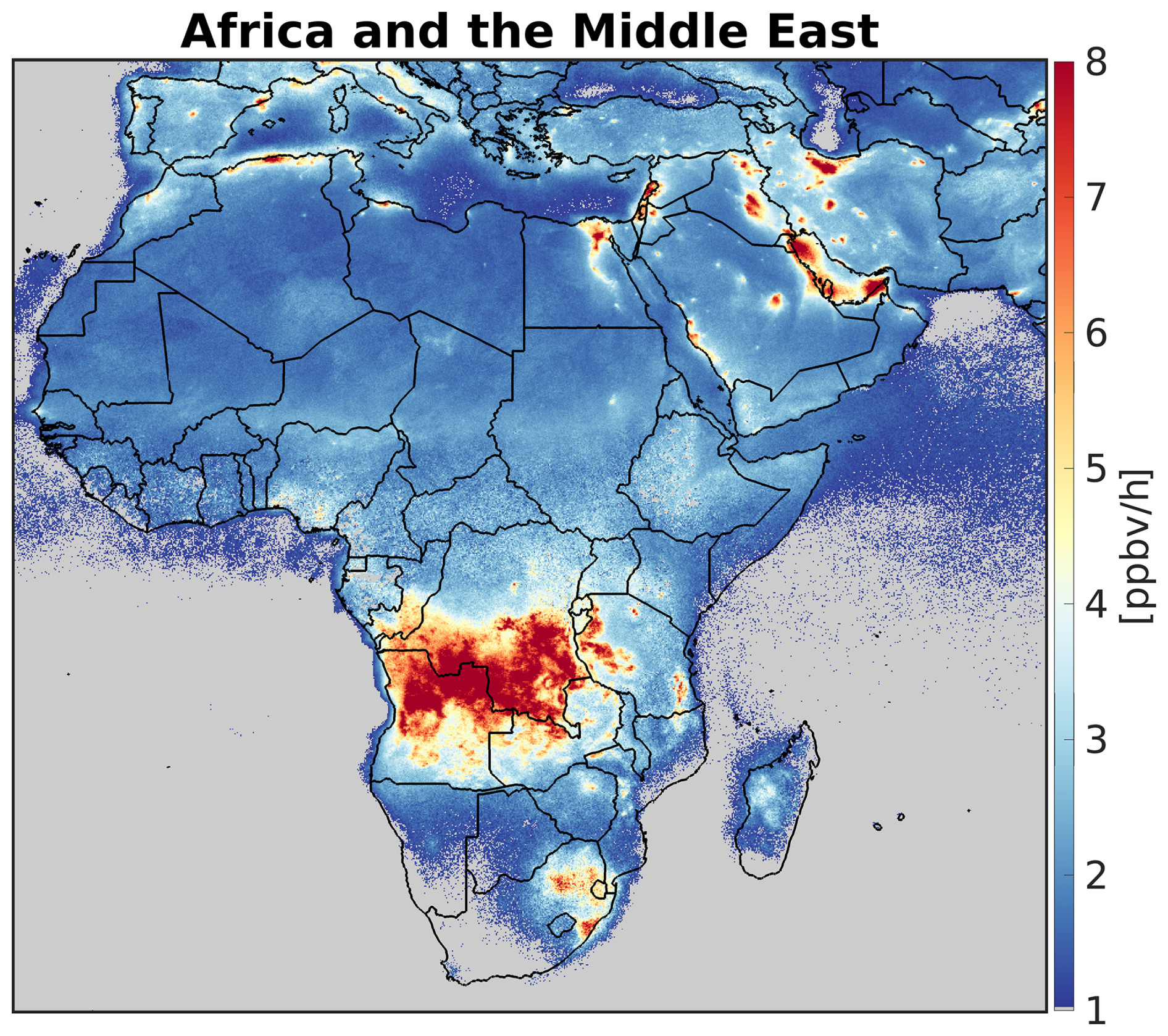
Figure 9 Spatial distribution of PO₃ within the PBL region, averaged over July 2019, for Africa and the Middle East. PO₃ < 1 ppbv h⁻¹ is masked due to algorithm deficiencies. Accelerated PO₃ rates can be seen over major cities and regions of biomass-burning activity in Africa.

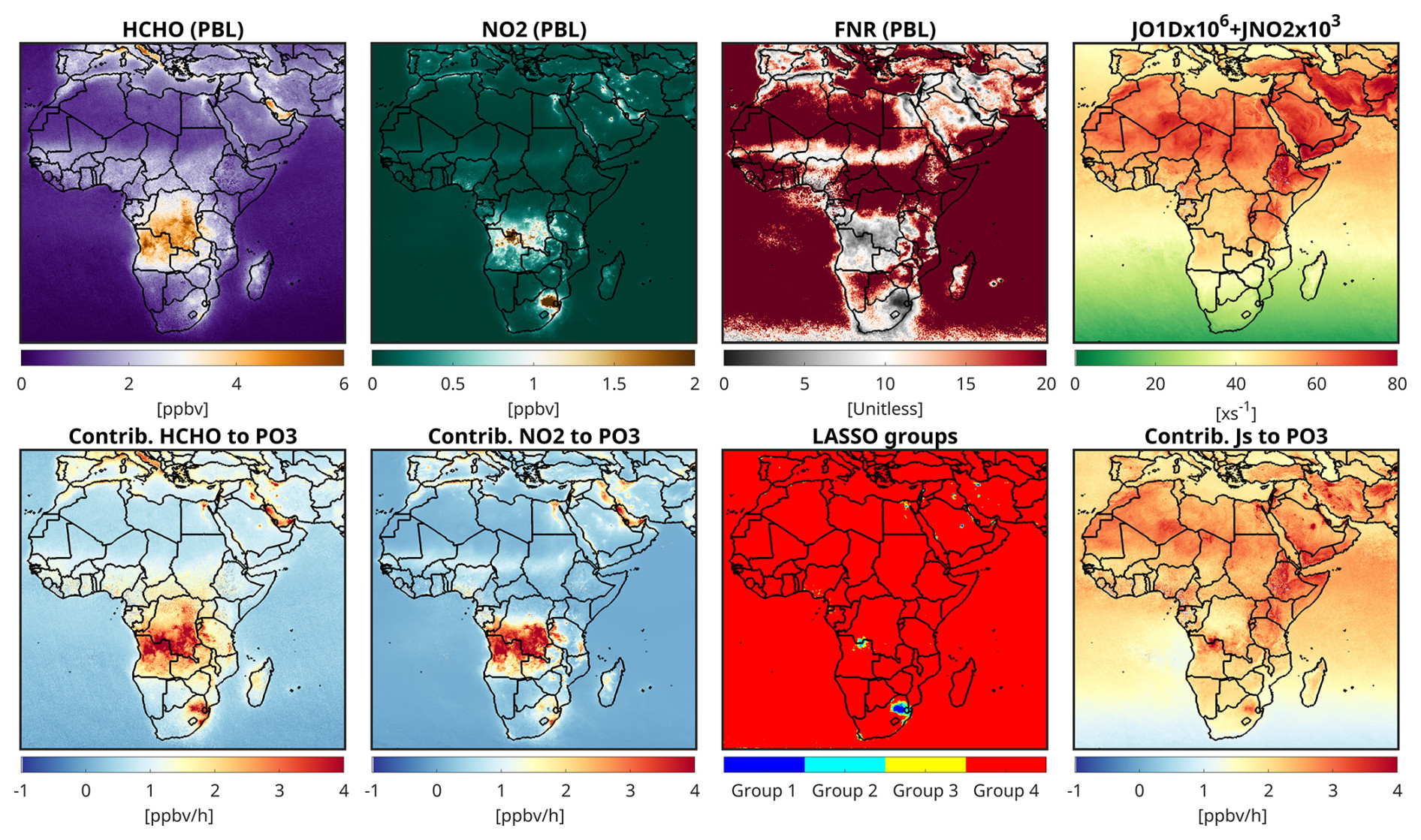
Figure 10 The first row shows the PBL concentrations of HCHO, NO₂, and FNRs, as well as the sum of scaled jO¹D and jNO₂, derived from TROPOMI and models with respect to July 2019. The second row shows the contributions of HCHO, NO₂, and photolysis rates to PO₃, along with the defined LASSO ozone production sensitivity regimes for PO₃ estimates. Contrib: contribution. J_s: photolysis rate.

Contiguous United States (CONUS). New York City, Los Angeles (LA), the San Francisco Bay Area, and Lake Michigan all experienced accelerated PO₃ rates in July 2019, as shown in Fig. 11. All these regions fall into non-attainment areas (marginal to extreme) with respect to ozone standards and have been extensively studied (Wu et al., 2024; Kim et al., 2022; Stanier et al., 2021). A robust relationship between PO₃ and ozone concentrations can only be established by factoring in physical processes such as horizontal and vertical transport, dry-deposition rates, and background values. In regions with high background ozone concentrations – for example, mountainous areas – even a moderate level of PO₃ can elevate ozone concentrations to unhealthy levels. Conversely, if there is a strong correlation between PO₃ and frequent ozone exceedances, such as those observed in the mentioned US cities, this indicates that locally produced ozone from chemical reactions is the primary factor contributing to such events. Except for LA, the vast majority of the CONUS exhibits large FNRs (> 3.5), meaning NO₂ levels largely shape the spatial distribution of PO₃ (Fig. 12). HCHO levels are found to be relatively large over LA, causing PO₃ to increase due to its greater sensitivity to VOCs. In addition to high levels of HCHO and NO₂ in several Californian regions, accelerated photochemistry caused by the bright surface albedo enhances PO₃.

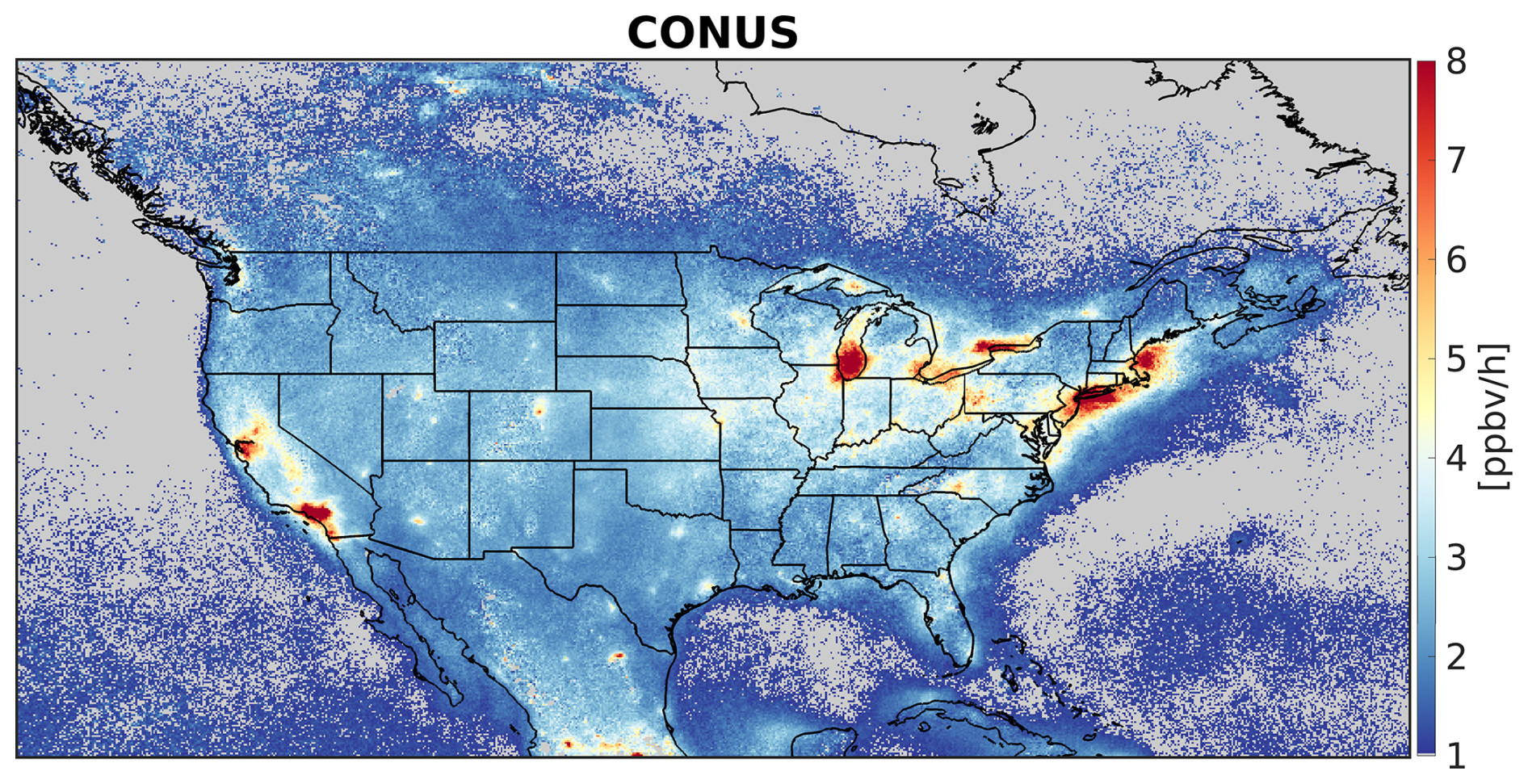
Figure 11 As in Fig. 9 but for the CONUS. Elevated PO₃ prevails over various areas, such as New York City, Los Angeles, the San Francisco Bay Area, and Lake Michigan.

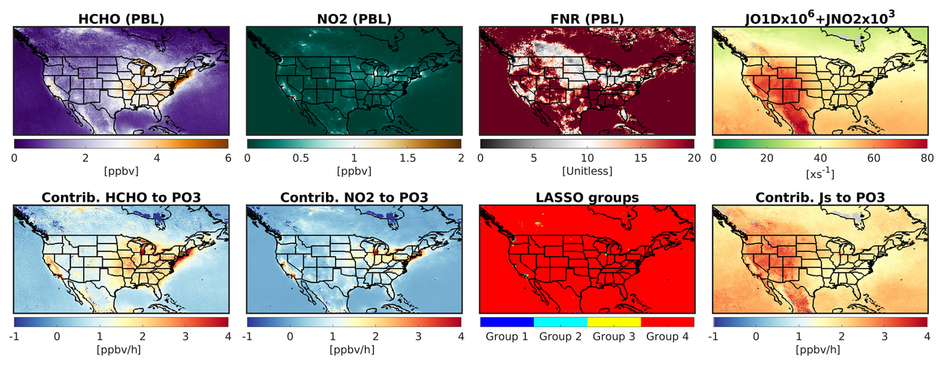
Figure 12 As in Fig. 10 but for the CONUS.

Eastern and southeastern Asia. Figure 13 shows extremely accelerated PO₃ rates over eastern Asia, particularly over the North China Plain, the Yangtze River Delta, the Pearl River Delta, and Seoul. These regions have experienced severely degraded air quality with respect to ozone (Souri et al., 2020a, b; Li et al., 2019; Colombi et al., 2023; Schroeder et al., 2020; Wang et al., 2017; Zhang et al., 2007). In southeastern Asia, Hanoi (Vietnam), Kuala Lumpur (Malaysia), and Jakarta (Indonesia) – which have also experienced heightened PO₃ – have received less attention in the literature (Ahamad et al., 2020; Kusumaningtyas et al., 2024; Sakamoto et al., 2018). Figure 14 suggests that the chemical conditions of many regions in China and South Korea, falling within the transitional regimes (LASSO groups 2 and 3 – 1.5 < FNR < 3.5), have made them susceptible to high PO₃ levels due to concurrently high concentrations of HCHO and NO₂. Moreover, photochemistry appears to be active throughout the region.

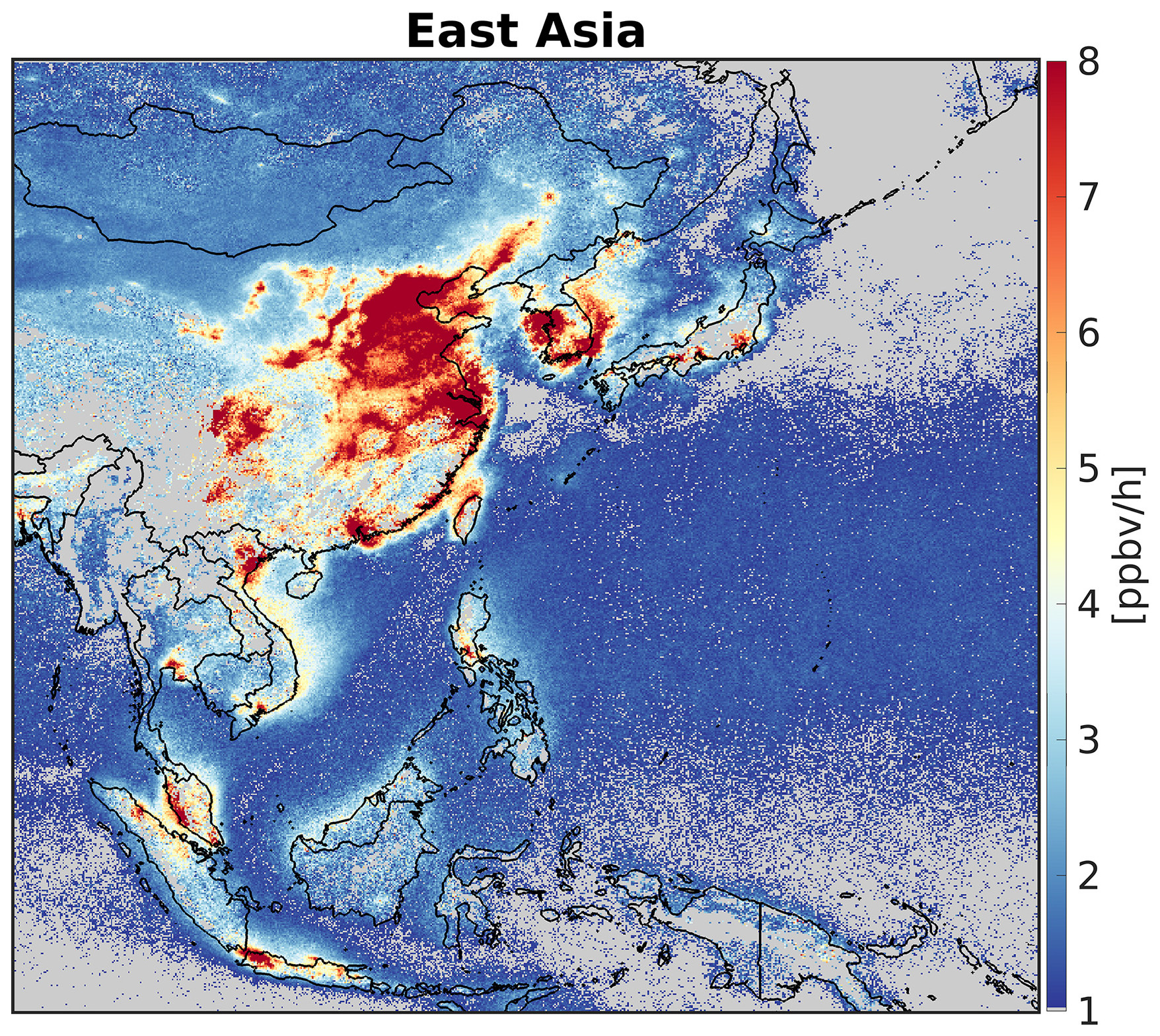
Figure 13 As in Fig. 9 but for eastern and southeastern Asia. Due to heightened levels of photochemistry, NO₂, and HCHO, we observe accelerated PO₃ rates across the majority of the cities in eastern and southeastern Asia.

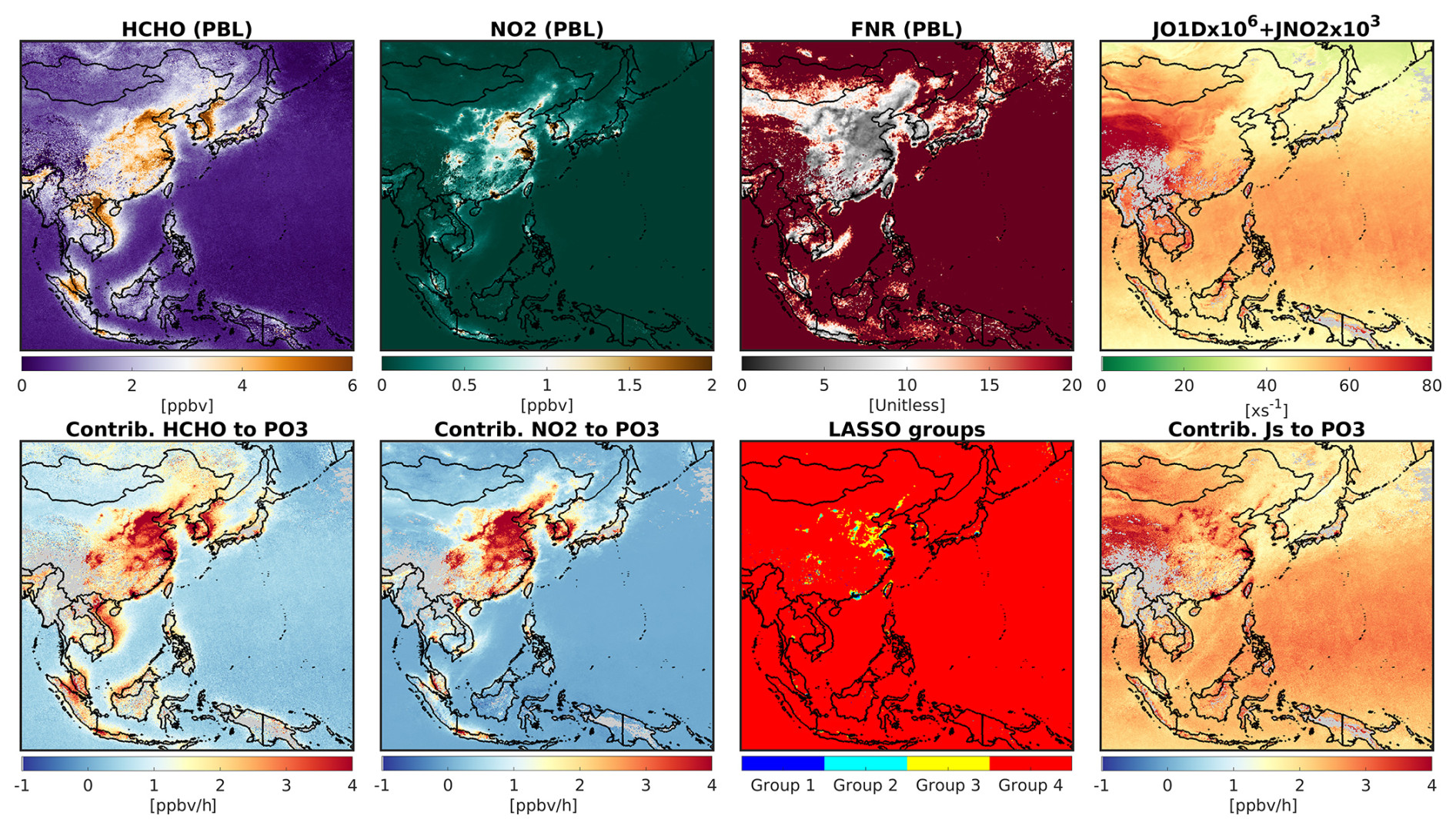
Figure 14 As in Fig. 10 but for eastern and southeastern Asia.

Europe. Figure 15 reveals high PO₃ levels over Benelux (Belgium, the Netherlands, and Luxembourg); the Po Valley (Italy); and several major cities, such as Barcelona (Spain) and Rome (Italy). Benelux exhibits the largest hotspot of PO₃ in the region (e.g., Zara et al., 2021). Benelux and a significant portion of England fall into the VOC-sensitive or transitional regimes (FNR < 2.5), as shown in Fig. 16. Due to diminished photochemistry in these high-latitude regions, we do not observe significant PBL concentrations of HCHO that would allow for PO₃ levels to be as high as in the previous areas; moreover, non-linear NO_x feedback has led to negative contributions of NO₂ to PO₃ in several cities, such as London. In general, low photolysis rates compared to the aforementioned regions have made most of Europe less prone to elevated PO₃.

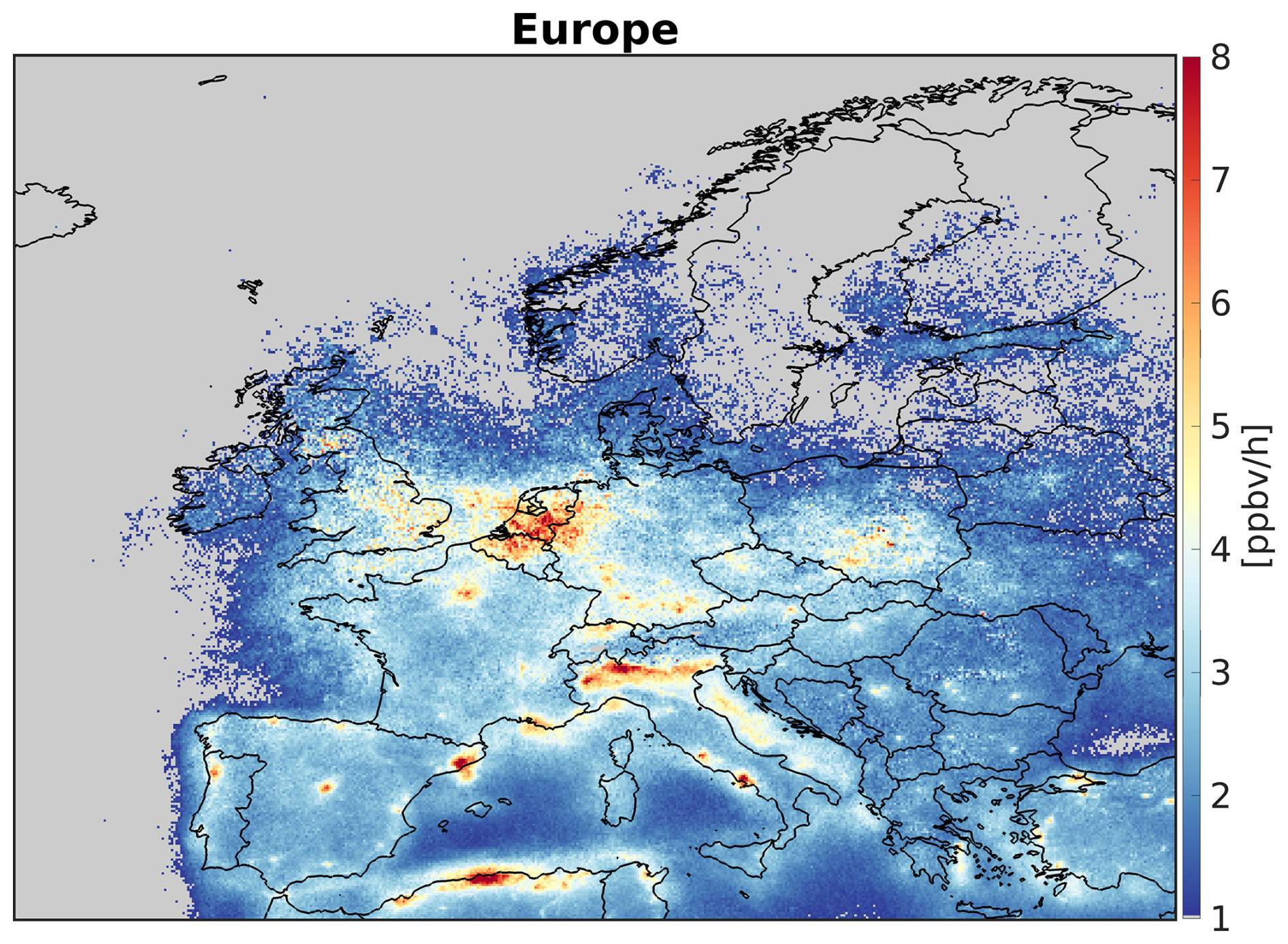
Figure 15 As in Fig. 9 but for Europe. Due to reduced photochemistry, PO₃ values tend to be smaller than in the previous cases. Benelux experiences the highest PO₃ levels in this region.

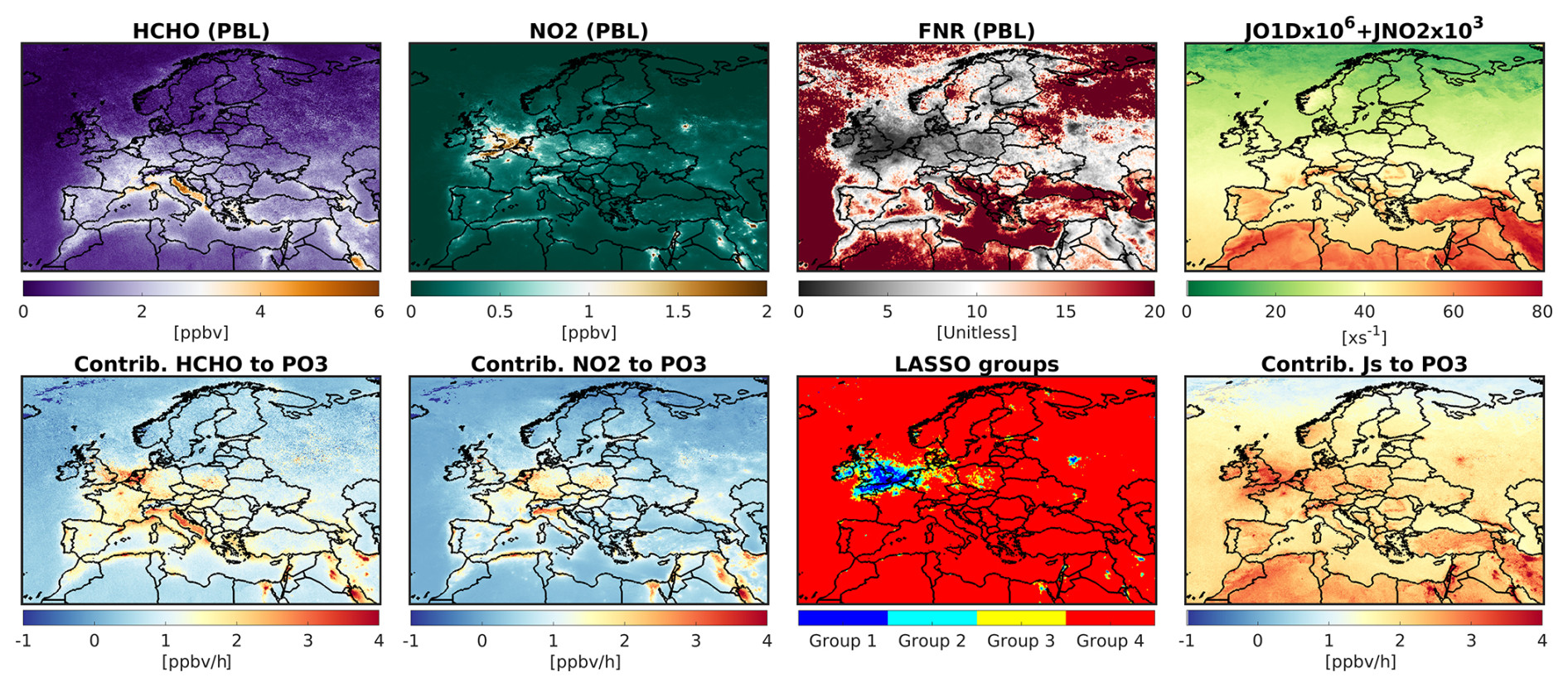
Figure 16 As in Fig. 10 but for Europe.

4.3.5 Seasonality of PO₃ over the Middle East

It is valuable to study the seasonal variations in the contributors to PO₃ over several major cities because the seasonality of PO₃ drivers can vary from location to location. We decided to focus on several Middle Eastern regions that have experienced rapid growth and deteriorating air quality: Cairo (Egypt), Gaza (Palestine), Baghdad (Iraq), Riyadh (Saudi Arabia), Tehran (Iran), and the Persian Gulf. We illustrate the seasonality of the four major contributors to PO₃ – NO₂, HCHO, jNO₂, and jO¹D – with respect to 2019 in Fig. 17.

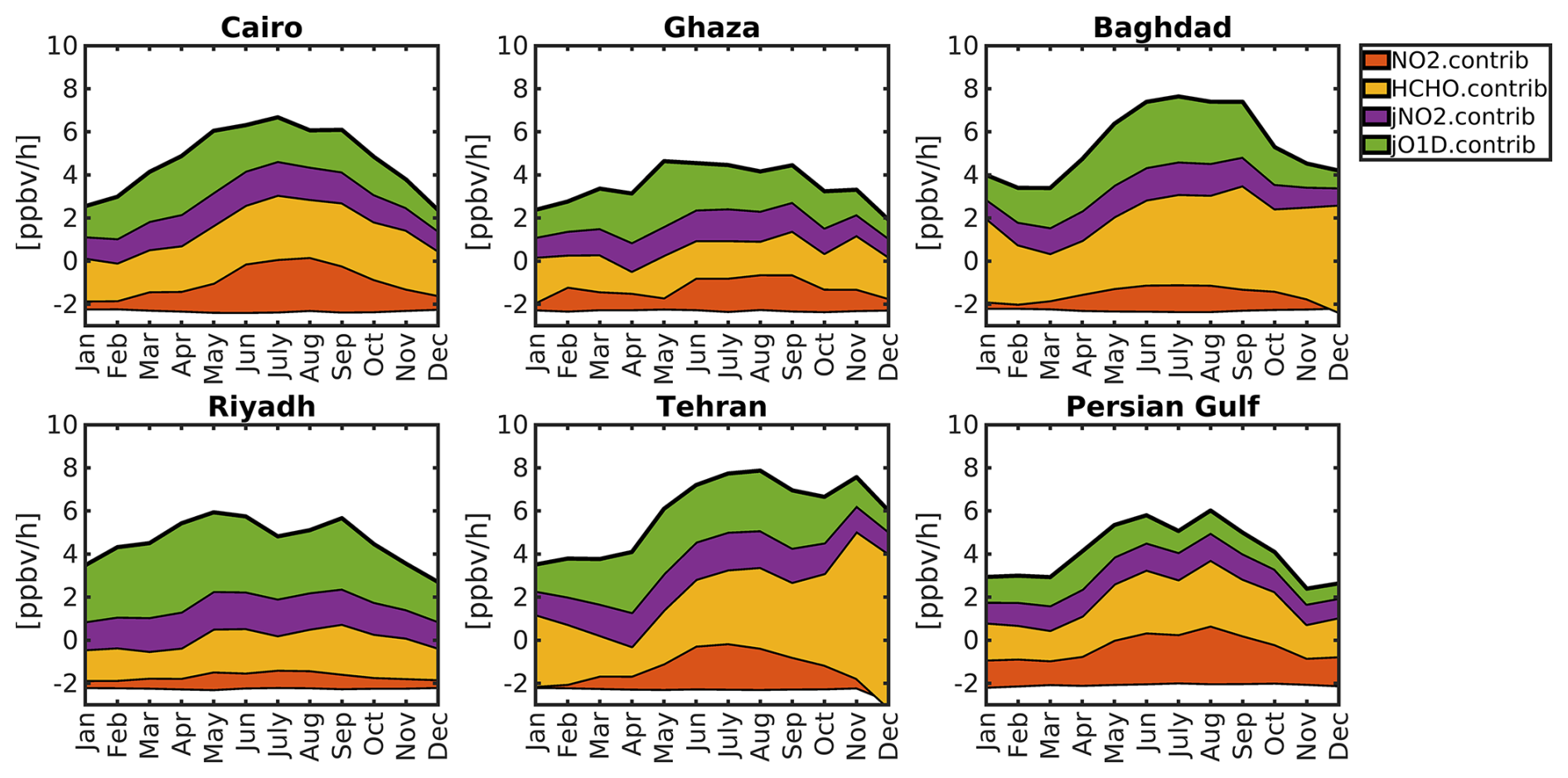
Figure 17 The contributions of NO₂, HCHO, jNO₂, and jO¹D to PBL PO₃ for several major regions in the Middle East. These estimates are based on the proposed algorithm, which integrates TROPOMI, ground-based remote sensing, and atmospheric models to estimate PO₃ using a statistical approach. PO₃ tends to spike during summer due to increased HCHO levels, a higher sensitivity of PO₃ to NO_x, and enhanced photochemistry. However, Tehran shows a second peak in fall due to unusually high values of HCHO.

HCHO levels (a proxy for VOCs) consistently have the greatest impact on PO₃ throughout the year in these regions. Specifically, both Baghdad and Tehran experience high levels of HCHO, even during the colder months, which can be observed using TROPOMI. This suggests that regulations targeting the reduction of human-made VOC emissions should be prioritized in these regions. PO₃ levels over Cairo, Gaza, Baghdad, and the Persian Gulf peak during summertime, while Tehran experiences a comparable peak in fall due to increased VOC emissions. Additionally, we notice a decrease in PO₃ levels over the Persian Gulf and Riyadh in July, possibly due to a decline in HCHO contributions caused by meteorological factors. Even though NO₂ concentrations decline in the summertime due to shorter lifetimes against OH, the higher amount of HCHO makes PO₃ more sensitive to NO₂ during this season. Gaza exhibits the least seasonal variation among these regions, likely due to consistently active photochemistry throughout the year.

4.3.6 The effect of satellite errors on PO₃

Satellite retrieval errors have been identified as the primary obstacle to achieving a robust understanding of ozone chemistry using HCHO and NO₂ data (Souri et al., 2023; Johnson et al., 2023); therefore, generating uncertainty maps is crucial for informing the scientific community about the credibility of our PO₃ estimates. In this study, we utilize the equations outlined in Sect. 2.2 to propagate the errors in HCHO and NO₂ retrievals to the final PO₃ estimates. We achieve this by recalculating the PO₃ value for a given pixel 10 000 times, with each recalculation based on a sample drawn from a normal distribution with a standard deviation equal to the satellite's total error. The standard deviation of these samples offers a good approximation of the impact of satellite errors on PO₃ estimates.

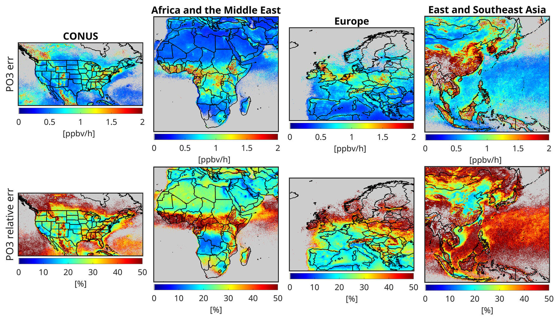
Figure 18 The influence of satellite errors on PO₃ estimates (both absolute and relative) over four major regions addressed in this work. The errors are based on monthly averaged TROPOMI errors. The errors tend to be mild over polluted regions (10 %–20 %), but they can exceed 50 % over pristine regions. Note that “err” stands for error.

Figure 18 illustrates the maps of absolute and relative PO₃ errors over the targeted regions for the month of July. The errors in the PO₃ estimates tend to be high (> 50 %) in remote regions, where the trace gas signals are small. However, the PO₃ errors are within 10 %–20 % in polluted regions, where the signals are larger. Currently, the absence of absolute measurements of PO₃ across this vast spatial coverage makes it challenging to assess the severity of these errors for PO₃ applications. Nonetheless, any application based on this product should be recalculated within the reported errors using a Monte Carlo approach to gauge the significance of the outcome.

5 Conclusion

Providing data-driven and integrated maps of the ozone production rate (PO₃) using a synergy of satellite retrievals, ground-based remote sensing, and atmospheric models enabled us to generate the first satellite-informed product of its kind, offering extensive spatial coverage and important applications for atmospheric chemistry. These data have indeed extended the use of the ratio of formaldehyde (HCHO) to nitrogen dioxide (NO₂), known as the FNR, beyond its current role. Through this product, we can shed light on the effects of emission regulations, wildfires, widespread lockdowns, wars, and economic recessions on PO₃ levels. Furthermore, using long-term records of satellite observations (e.g., those from OMI, starting in 2005, and TROPOMI, from 2018 onward), this product can inform emission regulators about locally produced ozone hotspots and, ultimately, enhance our understanding of the spatiotemporal variability in ozone formation over the past 2 decades.

In this study, we generated PO₃ maps within the planetary boundary layer (PBL), constrained by bias-corrected TROPOspheric Monitoring Instrument (TROPOMI) observations, using a piecewise regularized regression model. This model was calibrated using a blend of data from a comprehensive suite of aircraft observations and a well-characterized box model. These maps, produced for various regions, allowed us to identify hotspots of locally produced ozone pollution with unprecedented resolution. Our findings indicate that numerous urban areas in the Middle East, eastern Asia, and southeastern Asia exhibit accelerated PO₃ rates (> 8 ppbv h⁻¹), attributed to high levels of anthropogenic nitrogen oxides (NO_x = NO + NO₂), volatile organic compounds (VOCs), and active photochemistry. In contrast, such elevated PO₃ levels were less prevalent in the United States and Europe, with exceptions including Los Angeles, New York City, and the entire region of Benelux. Additionally, biomass-burning activities in Africa contributed to high PO₃ rates across extensive areas. The seasonality of PO₃ peaked around summer in several regions in the Middle East due to active photochemistry and concurrently high HCHO and NO₂ levels; however, Tehran experienced elevated PO₃ during fall due to large HCHO values, possibly produced from anthropogenic emissions.

The production of these maps relied heavily on a robust training dataset. To this end, we incorporated an extensive array of aircraft observations from multiple atmospheric composition campaigns, including DISCOVER-AQ, KORUS-AQ, INTEX-B, ATom, and SENEX, into the Framework for 0-D Atmospheric Modeling (F0AM) photochemical box model. This box model demonstrated a high level of correspondence (R² > 0.6, with minimal biases) between several unconstrained compounds (e.g., HCHO, OH, HO₂, PAN, NO, and NO₂) and their observed counterparts, indicating its effectiveness in understanding local ozone chemistry. Utilizing a classification algorithm applied to the data obtained from the constrained box model, we identified HCHO; NO₂; the ratio between HCHO and NO₂ (known as the FNR); photolysis rates; and, to some extent, meteorological factors as good candidates for reproducing PO₃ variability and magnitudes.

Subsequently, we employed a piecewise linear model known as LASSO, which performs feature selection by eliminating unimportant inputs, to parameterize PO₃. A key component of this parameterization was the use of FNRs to empirically linearize the non-linear ozone chemistry. The LASSO algorithm indicated that more than 88 % of the variance in PO₃ could be reproduced with low bias using only five parameters: the FNR, HCHO, NO₂, jNO₂ (the photolysis rate for NO₂ + hν), and jO¹D (the photolysis rate for O₃ + hν). This parameterization demonstrated remarkable performance for the majority of air parcels collected in moderately to extremely polluted regions (PO₃ > 1 ppbv h⁻¹). However, it performed poorly in pristine regions due to the exclusion of certain ozone loss pathways, such as HO_x (OH + HO₂), which are more challenging to predict.

Fortunately, TROPOMI provides critical data for enhancing the representation of the FNR, HCHO, NO₂, jNO₂, and jO¹D. We utilized TROPOMI's viewing geometry, UV surface albedo, and total ozone overhead from a model to predict jNO₂ and jO¹D, using lookup tables derived from NCAR's TUV model. To convert TROPOMI tropospheric NO₂ and HCHO columns into their corresponding PBL mixing ratios, we employed the MERRA-2 GMI global transport model, which is extensively used in various studies. However, the coarse resolution of this model might have introduced underrepresentation issues, which could be mitigated in future research by using higher-spatial-resolution models.

To address the biases associated with the TROPOMI observations, we updated comparisons from Verhoelst et al. (2021) and Vigouroux et al. (2020) with a larger dataset of paired TROPOMI–FTIR and TROPOMI–MAX-DOAS measurements. TROPOMI retrievals significantly underestimated HCHO and NO₂ magnitudes in polluted regions (exhibiting slope values of ∼ 0.6–0.7) and moderately overestimated them in pristine areas. These biases were corrected using regression lines, enabling a relatively unbiased application of the data.

To build confidence in our product, we propagated TROPOMI HCHO and NO₂ errors to PO₃ estimates using a Monte Carlo approach. The results indicated that PO₃ estimates were uncertain (> 50 %) in clean regions due to a low trace gas signal in TROPOMI retrievals. However, in polluted regions, the errors were more moderate (10 %–20 %) due to the stronger signal.

Over the years, extensive efforts have been devoted to measuring various critical atmospheric compounds globally, developing robust atmospheric models, and enhancing satellite retrievals and their benchmarks. These advancements have enabled us to estimate PO₃ maps within the PBL. Nonetheless, it is crucial to acknowledge some limitations of our work, many of which are the focus of ongoing research within our team:

• i.

  Direct measurements of PO₃ using specialized instruments (Cazorla and Brune, 2010; Sadanaga et al., 2017; Sklaveniti et al., 2018) are lacking in most atmospheric composition datasets, limiting our ability to fully understand the effects of assumptions made in the box model (such as the exclusion of heterogeneous chemistry) on PO₃.

• ii.

  There is potential for improvement in the parameterization process by employing more sophisticated algorithms, such as neural networks, which could increase the explained variance in the predicted PO₃.

• iii.

  The conversion of satellite column data to PBL mixing ratios requires error characterization and the use of finer-resolution models that are comparable in size to the PO₃ grid boxes.

• iv.

  Partially cloudy pixels and aerosols can affect photolysis rates, which should be considered in future parameterization efforts.

It is important to recognize that PO₃ maps are just one piece of the puzzle when it comes to determining ozone concentrations. Several studies have indicated that accurately representing surface ozone is challenging due to difficulties in representing background ozone, transport, and dry-deposition rates (e.g., Zhang et al., 2023; Clifton et al., 2020). Therefore, we advise against directly linking high PO₃ rates from our product to increased unhealthy ozone exposure. However, our product does provide indications as to whether heightened ozone concentrations are associated with chemistry contributions as opposed to other processes (e.g., meteorology or dry-deposition rates). Further investigation using additional tools/data is necessary to gather a full picture of these processes.

Despite these limitations, our novel product is a valuable asset to the atmospheric science community. It provides a more comprehensive understanding of the complexities associated with spatiotemporal variability in non-linear ozone chemistry over a large domain and enhances confidence in high-resolution maps of chemically produced ozone hotspots.