BVOC and speciated monoterpene concentrations and fluxes at a Scandinavian boreal forest

Boreal forests emit terpenoid biogenic volatile organic compounds (BVOCs) that significantly affect atmospheric chemistry. Our understanding of the variation of BVOC species emitted from boreal ecosystems is based on relatively few datasets, especially at the ecosystem-level. We conducted measurements to obtain BVOC flux observations above the boreal forest at the ICOS (Integrated Carbon Observation System) station Norunda in central Sweden. The goal was to study concentrations and fluxes of terpenoids, including isoprene, speciated monoterpenes (MTs), and sesquiterpenes (SQTs), during a Scandinavian summer. Measurements (10 Hz sampling) from a Vocus proton-transfer-reaction time-of-flight mass spectrometer (Vocus PTR-ToF-MS) were used to quantify a wide range of BVOC fluxes, including total MT (386 (± 5) ng m⁻² s⁻¹; β=0.1 °C⁻¹), using the eddy-covariance (EC) method. Surface-layer gradient (SLG) flux measurements were performed on selected daytime sampling periods, using thermal-desorption adsorbent tube sampling, to establish speciated MT fluxes. The effect of chemical degradation on measured terpenoid fluxes relative to surface exchange rates ($F/E$) was also investigated using stochastic Lagrangian transport modeling in forest-canopy. While the effect on isoprene was within EC-flux uncertainty ($F_{\mathrm{ISO}}/E_{\mathrm{ISO}}$ <  5 %), the effect on SQT and nighttime MT was significant, with average $F/E$ ratios for nighttime $F_{\mathrm{MT}}/E_{\mathrm{MT}}=$ ca. 0.9 (0.87–0.93), nighttime $F_{\mathrm{SQT}}/E_{\mathrm{SQT}}=\mathrm{0.35}$ (0.31–0.41), and daytime $F_{\mathrm{SQT}}/E_{\mathrm{SQT}}=\mathrm{0.4}$1 (0.37–0.47). The main compounds contributing to MT flux were α-pinene and Δ³-carene. Summer shifts in speciated MT emissions for Δ³-carene were detected, featuring a decrease in its relative fraction among observed MT compounds from June to August sampling periods, indicating that closer attention to seasonality of individual MT species in BVOC emission and climate models is warranted.

1 Introduction

Biogenic volatile organic compounds (BVOCs) play a central role in tropospheric chemistry, influencing both regional air quality and global climate (Fall, 1999). Many BVOCs participate in new particle formation (NPF) and growth (Bianchi et al., 2016; Boucher et al., 2013; Kirkby et al., 2016; Mohr et al., 2019; Riipinen et al., 2012; Tunved et al., 2006; Went, 1960). As BVOCs react with ozone, OH, and NO₃ (in the case of nighttime chemistry), the subsequent reaction products often have lower volatility that in suitable conditions can condense into new secondary organic aerosol (SOA) particles or contribute to the growth of existing aerosol particles (Bonn et al., 2009; Hallquist et al., 2009; Hodzic et al., 2016; Kulmala et al., 2004). BVOCs also affect the production and lifetime of tropospheric ozone through their photo-oxidation in the presence of NO_x, as well as through their interactions with OH and other radicals (Atkinson and Arey, 2003). As reactive BVOCs compete with methane for reacting with ambient OH, they may also have an influence on the atmospheric lifetime of this greenhouse gas (e.g., Kaplan et al., 2006). Oxygenated VOCs, such as acetone – one of the most abundant in the atmosphere (e.g., Singh et al., 1994), can also modify OH concentrations in the upper troposphere (Fehsenfeld et al., 1992; McKeen et al., 1997; Monks, 2005) and/or contribute to the formation of PAN that can act as a reservoir for NO_x (Read et al., 2012; Roberts et al., 2002).

Globally, BVOC emissions are several times greater than anthropogenic emissions, accounting for up to ca. 90 % of total VOC emissions worldwide (Guenther et al., 1995; Müller, 1992). In densely populated European regions, anthropogenic VOC emissions are estimated to exceed biogenic emissions, but in most cases, particularly those areas which are sparsely populated, biogenic emissions are dominant (Lindfors and Laurila, 2000; Simpson et al., 1999). These include sparsely populated countries in the European boreal zone (Simpson et al., 1999). The boreal vegetation zone, one of the Earth's largest terrestrial biomes and forming a near-continuous band around the Northern Hemisphere, is one of the major sources of BVOCs to the atmosphere at the global scale (Guenther et al., 1995; Sindelarova et al., 2014). Across all plant functional types (e.g., Guenther et al., 2012), boreal monoterpene (MT) emissions make up as much as ca. 26.3 % of the global summertime MT emission inventory (June: 28.3 %, July: 29.7 %, and August: 20.7 %), and up to ca. 37.1 % of it (June: 39.2 %, July: 41 %, and August: 30.5 %) for the Northern Hemisphere (Sindelarova et al., 2022).

Terpenoid compounds are an important fraction of BVOCs emitted globally (Guenther et al., 1995) and also from boreal forests (Rinne et al., 2009), and include isoprene (C₅H₈), the MTs (C₁₀H₁₆), the sesquiterpenes (SQTs; C₁₅H₂₄), and so on to diterpenes and larger compounds. Typically, for European boreal forests such as those largely composed of Scots pine and Norway Spruce (Rinne et al., 2009), isoprene emissions are relatively low while MT emissions predominate during typical ambient conditions (Hakola et al., 2006; Hakola et al., 2017), with isoprene emission about 10 %–15 % of MT emissions by mass (Rinne et al., 2009). When under significant stresses such as insect herbivory or drought, boreal forests are also known to be significant SQT emitters (Rinne et al., 2009; Niinemets, 2010). Isoprene is mainly involved in influencing production and lifespan of tropospheric ozone (Atkinson and Arey, 2003) but is relatively ineffective at enhancing tropospheric SOA yields compared to MT. In the lower troposphere, isoprene can even inhibit SOA NPF and early-stage particle growth, such as when present as an isoprene + MT mixture relative to a pure MT mixture (e.g., Heinritzi et al., 2020; Kiendler-Scharr et al., 2009; McFiggans et al., 2019). However, MTs as such emitted by the boreal forest biome are mainly involved in SOA particle formation and growth (Spracklen et al., 2008).

Globally, α-Pinene, β-pinene, and limonene typically have the highest net atmospheric abundance for MTs. Many MT isomers, however, are present and vary widely in structure (Geron et al., 2000; Guenther et al., 2012). In boreal forests, the emission of MT from predominant tree species, particularly Scots pine and Norway spruce, can vary as distinct chemotypes (referred to as α-pinene and Δ³-carene types) (Hiltunen and Laakso, 1995; Holzke et al., 2006; Janson, 1993; Komenda and Koppmann, 2002; Manninen et al., 2002; Tarvainen et al., 2005). The chemical speciation of MT emissions can also vary significantly within the same tree species population (e.g., Persson et al., 2016). This has direct effects on the resulting atmospheric chemistry, as MT reactivity and SOA formation potential varies by isomeric structure (Friedman and Farmer, 2018; Griffin et al., 1999; Lee et al., 2006a; Zhao et al., 2015). For example, Lee et al. (2006b) reported SOA yields from ozonolysis of MTs ranging from 17 % for β-pinene to 54 % for Δ³-carene (41 % for α-pinene) and in photolysis experiments (Lee et al., 2006a) found that Δ³-carene had an SOA mass yield that is ca. 16 %–30 % and 15 %–22 % greater than that of β-pinene and α-pinene, respectively. Accurately characterizing the speciation of MT fluxes from boreal forests is therefore of significant importance to parameterizing chemical species-specific emission factors in current and future climate and air quality models.

Observations of BVOC concentration above forest canopy are important for interpreting atmospheric chemistry processes, particularly in the lower troposphere and surface boundary layer directly above the forest, which are dependent on the concentration of precursor BVOC compounds (Atkinson, 2000; Pryor et al., 2014; Tunved et al., 2006). Observed concentrations are affected by both BVOC emission rate and micrometeorological conditions in the surface boundary layer (e.g., Karl et al., 2004; Petersen et al., 2023), as well as the chemical lifetime of relatively short-lived BVOC compounds (Atkinson and Arey, 2003). Very brief chemical lifetimes, such as for SQTs (τ_SQT – seconds), can affect their observed above-canopy fluxes as well (e.g., Rinne et al., 2012). Evaluating the ecosystem–atmosphere exchange of reactive BVOCs in the absence of chemical degradation, and hence isolating the roles of surface emission, deposition, and physical transport from its effects, represents an important goal for separating the relative influences on BVOC ecosystem-scale surface exchange and physical transport processes from atmospheric chemistry. Meanwhile, BVOC flux observations are important for understanding BVOC exchange between forest ecosystems and the atmosphere. Quantifying fluxes is also important for accurately parameterizing the functional dependencies of BVOC emissions on environmental parameters, such as temperature and solar radiation, as well as non-constitutive influences on ecosystem-scale emissions such as drought and disturbance stress, for regional and global atmospheric chemistry models (e.g., Rinne et al., 2007; Taipale et al., 2011).

There are multiple methods used to measure BVOC concentrations and fluxes (Rantala et al., 2014; Rinne et al., 2021). Proton-transfer-reaction mass spectrometry (PTR-MS) has been widely used to study BVOCs in the atmosphere (e.g., Yuan et al., 2017; Lindinger et al., 1998). In this technique, proton-transfer reactions with H3O⁺ ions are used to ionize atmospheric VOCs for detection of the product ions by mass spectrometry. In recent years, it has become possible to perform eddy-covariance (EC) measurements of BVOC fluxes using fast-response (τ1 s) PTR time-of-flight MS (PTR-ToF-MS) over a wide range of BVOC molar masses (Müller et al., 2010). The EC flux approach, based on the covariance between fast (10–20 Hz) observations of the fluctuations in chemical concentration and vertical wind speed (see Sect. 2.4), has the advantage of being the most direct and accurate approach for measuring ecosystem-level BVOC fluxes, and thus is an important component for biosphere BVOC emission research. Fluxes measured by micrometeorological methods can be used to study the effects of environmental parameters on BVOC emissions. They can also be applied in up-scaling studies, where canopy-scale measurements provide an important intermediate step between leaf-level and regional-scale for use in model verification (Guenther, 2012; Peñuelas and Staudt, 2010; Rinne et al., 2009). A high sampling rate is essential to resolve fluctuations from small, short-lived eddies (0.1–5 Hz) that drive turbulent transport, as lower rates can lead to significant attenuation of measured fluxes due to unresolved turbulence. The high sampling rate capability of PTR-ToF-MS (>10 Hz) makes it well-suited for measuring BVOC fluxes using the EC method. Additionally, EC-based methods utilizing PTR-ToF-MS can be implemented for various mobile platforms, including aircraft, for spatially resolved landscape-scale flux assessments over wide areas (Pfannerstill et al., 2023). When combined with the high sensitivity and accuracy of modern instrumentation (e.g., Krechmer et al., 2018), PTR-ToF-MS stands as one of the most effective tools currently available for measuring ecosystem-scale BVOC fluxes. A limitation of PTR-MS analysis is, however, that it identifies compounds collectively by their mass-to-charge ratio, and cannot differentiate between compounds with the same molar mass and molecular composition (i.e., isomeric compounds). For example, MTs (C₁₀H₁₆), which can be emitted in a boreal forest as any one of many structurally unique compounds, all have a protonated nominal mass-to-charge ($m/z$) ratio of 137.130.

While BVOC flux studies have made great strides due the development of PTR instrumentation, improvements to the study of speciated MT fluxes are still lacking. In addition to total fluxes (such as total MT flux), speciated flux information can be used to further improve model verification for compound-specific emission potentials used in emission models (e.g., MEGAN) (Guenther et al., 2012). Methods used to measure speciated BVOC fluxes include variants of the gradient method (see Sect. 2.6), which assumes that a compound's ecosystem–atmosphere turbulent flux is proportional to its vertical concentration gradient above the forest canopy (where the proportionality constant is the turbulent exchange coefficient) (Fuentes et al., 1996; Goldstein et al., 1995; Guenther et al., 1996; Rinne et al., 2000a; Schween et al., 1997). By using automated thermal desorption (ATD) gas chromatograph–mass spectrometry (GC-MS) for adsorbent tube sampling of the vertical BVOC gradient, in conjunction with PTR-ToF-MS measurements of the EC-derived BVOC fluxes, the information from these two approaches to BVOC flux observations can provide additional insight into the ecosystem–atmosphere exchange of BVOCs between boreal forests and the troposphere.

In this work, concentrations and fluxes of BVOCs, particularly the MTs, at a Swedish site in the European boreal zone are presented. Six weeks of Vocus PTR-ToF-MS measurements were performed from 21 July to 26 August 2020. Thermal desorption (TD) tube samples of the BVOC concentration were collected during the daytime (typically between 09:00 am and 05:00 pm) at 37 m and 60 m a.g.l. on the Norunda flux tower over 3 d periods, during 8–10 June (prior to Vocus deployment), 22–24 July, and 16–18 August.

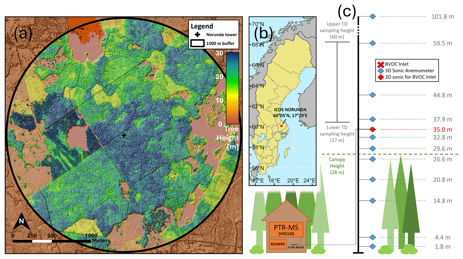
Figure 1 Forest map, station location, and BVOC inlet setup for ICOS Norunda. (a) A map of tree heights surrounding the station flux tower (out to 1500 m radially from tower base) for the Norunda forest. (b) Location and coordinates of ICOS station Norunda in Sweden. (c) BVOC inlet, infrastructure, and instrumentation setup for Vocus PTR-ToF-MS measurements on the Norunda tower (BVOC inlet at 35 m). Shown are the heights of the on-site collection of 3D sonic anemometers (blue diamonds) and BVOC inlet (red cross) at the station flux tower. The canopy top height was at approximately 28 m. Sonic-profile anemometers were located at 1.8, 4.4, 14.8, 20.8, 26.6, 29.6, 32.8, 35, 37.9, 44.8, 59.5, 74,88.5, and 101.8 m on the Norunda tower. The instrument shed contained the Vocus PTR-ToF-MS and zero-air generator for the Vocus. A blower was used to pull air through the tower inlet.

2 Methods

2.1 Measurement site

This study was conducted at the Norunda research station, located at 60°05^′ N, 17°29^′ E, ca. 30 km north of Uppsala, in central Sweden. The station is part of the Integrated Carbon Observation System (ICOS) research infrastructure (https://www.icos-cp.eu, last access: 14 October 2025; (Heiskanen et al., 2022)), a network for monitoring greenhouse gases and short-lived climate forcers (more recently, part of Aerosol, Clouds, and Trace Gases Research Infrastructure (ACTRIS) in Sweden (https://www.actris.eu, last access: 14 October 2025) as well). The station was surrounded by a mixed-conifer forest of Scots pine (Pinus sylvestris) and Norway spruce (Picea abies). This forest was between 80 and 120 years old (Lagergren et al., 2005) and the forest canopy height was ca. 28 m (Wang et al., 2017). The forest (subsequently clearcut in 2022 for lumber) has been managed for economic purposes for approximately the last 200 years. The research station has been in operation since 1994 as a CO₂ and trace gas flux station and is equipped with a 102 m tower (Lindroth et al., 1998; Lundin et al., 1999). A station map and its location in Sweden are presented in Fig. 1.

Together, Norway spruce (53.4 %) and Scots pine (39.8 %) make up 93.2 % of mean tree number per hectare. There was also a small number of deciduous trees, consisting primarily of black alder (Alnus glutinosa (L.) Gaertn; 2.5 %) and downy birch (Betula pubescens Ehrh.; 3.9 %). The dominant ground vegetation at the station was bilberry (Vaccinium myrtillus) and lingonberry (Vaccinium vitis-idaea), in addition to several species of dwarf shrubs, ferns, and grasses. The bottom layer vegetation predominantly consisted of a thick layer of feather moss (Pleurozium schreberi and Hylocomium splendens). During the 25 years prior to 2020, the mean monthly temperature varied between −5 and 25 °C, and the mean annual precipitation was approximately 540 mm. The growing season, with daily air temperatures above 5 °C, ranges typically from May to September. During the same calendar period as the collected 2020 Norunda campaign measurements (8 June–August 28), the local 25-year climatological average daily temperature was 16.4 ± 2.7 °C, with an average nighttime minimum of 10.7 ± 3 °C and daytime maximum of 21.2 ± 3.6 °C. New needle growth typically begins in April. Foliation of existing deciduous trees and plants usually occurs in May and senescence usually in October (± 15 d). From 2009 to 2014, the leaf area index (LAI) of the Norunda forest in proximity of the tower was determined to be approximately 3.6 (± 0.4) using a LAI 2000 (Li Cor Inc., Lincoln Nebraska, USA).

2.2 Instrumentation and sampling setup

The canopy temperature of the Norunda forest was measured using a precision SI-111 infrared radiometer (Campbell Scientific Inc., Logan UT, USA) mounted at 55 m on the station flux tower. The wind velocity components were measured using a three-dimensional sonic anemometer (USA-1, Metek GmbH, Germany). BVOC volume mixing ratios were measured using a Vocus PTR-ToF-MS (Vocus-2R, TOFWERK, Thun, Switzerland) (Krechmer et al., 2018). The Vocus has several advantages over previous PTR-ToF-MS designs, such as in detecting low-volatility BVOC compounds (Krechmer et al., 2018). The Metek sonic anemometer and BVOC sampling inlet were co-located at 35 m on the Norunda flux tower. Ambient air at 35 m was transported from the BVOC inlet head through a heated and insulated PFA Teflon tube mounted on the station flux tower (Fig. 1) to the instrument shed housing the Vocus PTR-ToF-MS using a side-channel blower. The tower Teflon tubing was ca. 49 m in length with an outer diameter of $\mathrm{3}/\mathrm{8}$ in (inner diameter $\mathrm{1}/\mathrm{4}$ in). The flow rate through the BVOC inlet tubing to the Vocus was 20 L min⁻¹ to minimize BVOC losses from prolonged residence time within sample tubing. Sample air residence time in tower Teflon tubing before reaching instrumentation was ca. 4.7 ± 1 s.

Inside the instrumentation shed, 6 L min⁻¹ of the flow coming from the main inlet tubing were directed to the Vocus inlet, and 100 mL min⁻¹ were sampled into the Vocus, and the remainder was directed to the inlet exhaust. The Vocus ion source was set at 2 mbar. From field measurements, the mass-resolving power ($m/\mathrm{\Delta }m$) of the Vocus, where Δm is the full-width at half-maximum (fwhm) of a spectrum peak, was found to be ca. 9900 Th/Th fwhm for the MT parent ion C₁₀H₁₆H⁺ (nominal $m/z=\mathrm{137}$). During the campaign, data from the Vocus were recorded at a frequency of 10 Hz. Reference measurements to determine the instrumental background of the Vocus PTR-MS were periodically performed (for 1 min each hour) using zero air from a heated catalytic converter (Zero Air Generator, Parker Balston, Haverhill, MA, USA). The mass flow controller for the Vocus zero-air was set to 500 mL min⁻¹. The Vocus calibration was performed using a gravimetrically prepared calibration standard (Ionimed Analytik, Innsbruck, Austria). The calibration standard gas was diluted before sampling by the Vocus using a gas calibration unit (GCU-b, Ionicon, Innsbruck, Austria).

2.3 Vocus data processing

For compounds present in the calibration gas standard bottle, the corresponding calibration factor was applied directly to the processed Vocus trace data. For the remaining compounds, calibration factors were calculated using the analysis approach implemented by the PTR data toolkit as described by Jensen et al. (2023) (See Table C2 of calibration coefficients and calculated terpenoid sensitivities). The fractionation rate estimate for SQTs (0.20 ± 0.1) is based on PTR Library reference of proton-transfer reactions in trace gas sampling (Pagonis et al., 2019).

The processing of the raw Vocus data was performed using Julia-based analysis scripts from the software package TOF-Tracer2 (Breitenlechner et al., 2017; Fischer et al., 2021; Stolzenburg et al., 2018), modified for use with the Vocus PTR-ToF-MS dataset. For each campaign day, all Vocus spectra data acquired within 24 h were mass-scale calibrated every 6 min and averaged for peak shape analysis. The program PeakFit (Fischer et al., 2021) was used for peak fitting and identification. PeakFit was used to create a mass peak list of more than 2000 identified compounds for our Vocus dataset. Based on this mass peak list and using the modified TOF-Tracer2 scripts, the 10 Hz time traces were obtained by integrating the spectra for intervals around each mass, then applying deconvolution to reduce cross-talk caused by signal contributions from neighboring masses and isotopes in each spectrum (Müller et al., 2010). The script runtime on a 10-core processor system with 1Tb hard drive and 96 GB of RAM is approximately 2.5 h for 24 h of 10 Hz data. The recorded amount of raw Vocus data collected each day in the native HDF5-file format was approximately 20 GB.

2.4 Eddy-covariance fluxes

The most direct method for measuring a chemical flux above a forest canopy is the EC method. It requires simultaneous, fast (10–20 Hz) measurements of the compound concentration (c) and vertical wind velocity (w). The covariance between the time-dependent fluctuations of these variables gives the flux (F_c), with

$$\begin{array}{}\text{(1)}& F_{\mathrm{c}}=\stackrel{\mathrm{‾}}{w{}^{\prime }c{}^{\prime }}={\displaystyle \frac{\mathrm{1}}{t_{\mathrm{2}}-t_{\mathrm{1}}}}\underset{t_{\mathrm{1}}}{\overset{t_{\mathrm{2}}}{\int }}w{}^{\prime }\left(t\right)c{}^{\prime }\left(t\right)\mathrm{d}t,\end{array}$$

where the overbar denotes time averaging from time t₁ to time t₂, $c{}^{\prime }=c-\stackrel{\mathrm{‾}}{c}$, and $w{}^{\prime }=w-\stackrel{\mathrm{‾}}{w}$. Further information regarding the EC approach can be found in the literature (e.g., Aubinet et al., 2012a). As a significant proportion of a turbulent flux in the atmospheric surface layer is carried by relatively small eddies, for the EC-flux method to accurately quantify the vertical exchange, the BVOC concentration and vertical wind speed must be measured by fast-response instrumentation. Typically, many analyzers for greenhouse gas fluxes have response times of around 0.1 s. While the PTR analyzer's characteristic response time τ (i.e., time for 100 × 1/e % ≈63.2 % of instrument signal to fully transition between two levels of concentration) is around 1 s, due to transit time of the BVOC product ions in the Vocus drift tube reaction chamber (Krechmer et al., 2018), the effect of this is relatively minimal for evaluating BVOC EC flux (high-frequency attenuation of total flux signal is about 1 %), and can be accounted for by a transfer function correction factor (Striednig et al., 2020). This is sufficient for fluxes measured above tall vegetation, such as forest canopies (Rantala et al., 2014).

The EC flux calculations were performed using the MATLAB-code innFLUX (Striednig et al., 2020). The analysis routines implemented in this code include a wind sector-dependent tilt correction, lag time determination, and calculation of several quality tests. In particular, a tilt-correction was performed on the Metek sonic data to align the instrument's coordinate system with the mean wind streamlines (e.g., Wilczak et al., 2001). The time delay between the Metek sonic and Vocus BVOC signals was determined by maximizing the correlation coefficient of the Vocus signals with the vertical wind component. For the final processing of the data points for the Vocus EC flux time series, 30 min ensemble averages were selected.

2.5 Adsorption sampling and ATD-GC-MS analysis

For a gradient-flux approach targeting the speciated MT fluxes, ambient air BVOC samples were collected over three-day periods, approximately once a month, from June to August, from two heights. These air samples were simultaneously collected at 37 and 60 m on the Norunda flux tower for 30 min periods, once an hour, starting at 09:30 am and concluded with the collection of the last sample-pair at 05:00 pm from the tower.

Air samples were collected using stainless steel TD tubes (10 cm in length and $\mathrm{1}/\mathrm{4}$ inch in diameter) and filled with Tenax GR and Carbograph 5TD (Markes International Inc., USA). Ambient air was pumped through these TD tubes at 200 mL min⁻¹ for 30 min (6 L total per sample) using flow-controlled sampling pumps (Pocket Pump Pro, SKC Ltd., Dorset, UK). Two MnO₂-coated copper mesh filters (50 mm grid, type ETO341FC003, Ansyco, Karlsruhe, Germany) were placed inside a Teflon inlet head affixed in front of each sampling tube, to remove ozone from the ambient air. In previous studies it was found that these MnO₂-coated mesh filters destroy about 80 % of the ozone but leave α-pinene, β-pinene, limonene, Δ³-carene, and other terpenoids intact (e.g., Bäck et al., 2012; Calogirou et al., 1996). TD samples were refrigerated and then analyzed within 30 d of collection. Calibration tubes were also prepared and analyzed to calibrate the subsequent GC-MS analysis (e.g., Bai et al., 2016).

TD tubes were thermally desorbed and cryo-focused using a Perkin Elmer TurboMatrix 650 ATD. This ATD was operated in splitless mode. Samples were then injected into a gas chromatograph–mass spectrometry system (GC-MS, Shimadzu QP2010 Plus, Shimadzu Corporation, Japan). For the gas chromatography portion of the ATD-GC-MS analysis, the BVOC gas samples were separated using a BPX5 capillary column (50 m, I.D. 0.32 mm, film thickness 1.0 µm, Trajan Scientific, Australia). The carrier gas was helium. The GC oven temperature program was as follows: start temperature, 40 °C; hold time, 1 min; ramp 1, 6 °C min⁻¹ to 210 °C; ramp 2, 10 °C min⁻¹ to 25 °C; final hold time, 5 min. The GC-MS was run simultaneously in both SIM and SCAN modes (e.g., Duhl et al., 2013). This choice was to enable detection of both common and unanticipated compounds. For sample calibration, a pure standard solution containing isoprene, α-pinene, β-pinene, p-cymene, eucalyptol, limonene, 3-carene, linalool, α-humulene, β-caryophyllene, longifolene, and myrcene (Merck KGaA, Darmstadt, Germany) was prepared in methanol. This standard solution was injected onto conditioned adsorbent sampling tubes in a helium stream, with cartridges receiving different concentrations of the standard solution. These prepared TD tubes were then analyzed with the samples to provide a calibration curve (e.g., Noe et al., 2012).

2.6 Gradient-method fluxes

In the surface-layer gradient (SLG) method we obtain the turbulent flux by using the vertical gradient of the measured volume mixing ratios (i.e., concentrations $\stackrel{\mathrm{‾}}{c}$) and a turbulent exchange coefficient K in the manner analogous to molecular diffusion, with $F_{\mathrm{c}}=-K\frac{\mathit{\delta }\stackrel{\mathrm{‾}}{c}}{\mathit{\delta }z}$. The turbulent exchange coefficient K can be obtained in several approaches, such as using results from another scalar quantity through the modified Bowen ratio approach or by application of Monin–Obukhov similarity theory (e.g., Rannik, 1998; Rantala et al., 2014). In the case of BVOC gradient sampling using TD tubes at two heights, we use the Monin–Obukhov similarity approach as in e.g., Fuentes et al. (1996) and Rinne et al. (2000b),

$$\begin{array}{}\text{(2)}& F_{\mathrm{c}}={\displaystyle \frac{-k{u}_{\ast }\left[\stackrel{\mathrm{‾}}{c}\left(z_{\mathrm{1}}\right)-\stackrel{\mathrm{‾}}{c}\left(z_{\mathrm{2}}\right)\right]}{\ln \left(\frac{z_{\mathrm{2}}-d}{z_{\mathrm{1}}-d}\right)+{\mathit{\psi }}_h\left(\frac{z_{\mathrm{1}}-d}{L}\right)-{\mathit{\psi }}_h\left(\frac{z_{\mathrm{2}}-d}{L}\right)}},\end{array}$$

where u_∗ is the friction velocity, d is the displacement height, L is the Obukhov length, ψ_h is the Monin–Obukhov stability function for heat, k is the von Kármán constant, and $\stackrel{\mathrm{‾}}{c}\left(z_{\mathrm{1}}\right)$ and $\stackrel{\mathrm{‾}}{c}\left(z_{\mathrm{2}}\right)$ are the BVOC concentrations at heights z₁ and z₂, respectively. The values of the integrated stability functions ψ_h were calculated using the Businger–Dyer equations (Dyer, 1974), with

$$\begin{array}{}\text{(3)}& \begin{array}{l}{\mathit{\psi }}_h=\mathrm{2}\ln \left(\frac{\mathrm{1}+Y}{\mathrm{2}}\right),\left(\mathrm{for}\mathit{\zeta }<\mathrm{0}\right),\\ {\mathit{\psi }}_h=-{\mathit{\beta }}_h\mathit{\zeta },\left(\mathrm{for}\mathit{\zeta }>\mathrm{0}\right),\end{array}\end{array}$$

where $\mathit{\zeta }=(z-d)/L$, and coefficients $Y=(\mathrm{1}-\mathrm{12}\mathit{\zeta }{)}^{\mathrm{1}/\mathrm{2}}$ and β_h=7.8 were selected based on those used in previous investigations (Businger et al., 1971; Dyer, 1974; Rannik, 1998; Rantala et al., 2014; Rinne et al., 2000a).

In the atmosphere directly above rough surfaces, such as forest canopy, flux-gradient laws tend to break down (Cellier and Brunet, 1992; Fazu and Schwerdtfeger, 1989; Garratt, 1980; Högström et al., 1989; Mölder et al., 1999; Simpson et al., 1998). The layer in which these laws are not directly applicable is called the roughness sublayer (RSL). In the RSL, the eddy diffusivities are increased, and consequently, vertical gradients are decreased compared to their non-dimensionalized gradient form, which for a scalar concentration C is expressed by ${\mathrm{\Phi }}_C\left(\mathit{\zeta }\right)=\frac{k(z-d)}{c_{\ast }}\frac{\partial \stackrel{\mathrm{‾}}{C}}{\partial z}$, where c_∗ is the scalar flux concentration (e.g., Rannik 1998). The decrease in gradients due to the influence of the RSL layer can be quantified and corrected for by using the non-dimensional factor γ, expressed as

$$\begin{array}{}\text{(4)}& \mathit{\gamma }={\displaystyle \frac{{\mathrm{\Phi }}_{\mathrm{S}}}{\mathrm{\Phi }}},\end{array}$$

where Φ_S is the dimensionless gradient of a scalar according to the Monin–Obukhov similarity theory (i.e., Eq. 4) and Φ is the dimensionless gradient according to the measurements. The observed γ-coefficients above a forest canopy at the heights our TD samples were collected typically vary from unity to 3 depending on the measurement height and type of the forest (e.g., Simpson et al., 1998).

From γ, it is possible to calculate a mean enhancement factor Γ by integrating the γ-coefficient from the measurement height z₁ to z₂ (e.g., Rinne et al., 2000b), such that in general we have

$$\begin{array}{}\text{(5)}& \mathrm{\Gamma }\left(z_{\mathrm{1}},z_{\mathrm{2}}\right)={\displaystyle \frac{\mathrm{1}}{z_{\mathrm{2}}-z_{\mathrm{1}}}}\left[\underset{z_{\mathrm{1}}}{\overset{z_{\mathrm{2}}}{\int }}\mathit{\gamma }\left(z\right)\mathrm{d}z\right].\end{array}$$

Details of the γ-coefficient profile analysis for the RSL above the Norunda canopy, as well as determination of displacement height d (24 m), are included in the Appendix. Based on this analysis, we have found a Γ-coefficient value of 1.36 ± 0.09 for TD gradient-flux calculation.

2.7 Gradient-method error analysis

For the two-point SLG gradient method, as alluded to by the form of $F_{\mathrm{c}}=-K\frac{\mathit{\delta }\stackrel{\mathrm{‾}}{c}}{\mathit{\delta }z}$ and Eq. (2), the sources of uncertainty can be divided into those from the gradient (i.e., measured concentration difference $\stackrel{\mathrm{‾}}{c}\left(z_{\mathrm{1}}\right)-\stackrel{\mathrm{‾}}{c}\left(z_{\mathrm{2}}\right))$ and those from to the turbulent exchange coefficient K. A detailed evaluation of SLG-related uncertainties for BVOC flux measurements is presented in Rinne et al. (2000b).

The adsorption sampling and analysis of the BVOCs represents the largest single source of uncertainty in the flux calculation. This is due to the relatively small difference in concentrations between sampling heights as compared to the uncertainty of the concentration measurements themselves. The two error sources which can be evaluated for the chemical gradient measurements are the sampling uncertainty and the analysis uncertainty from the ATD-GC-MS (e.g., Kajos et al., 2015). Measurement results from the ATD-GC-MS include values for peak area mean and standard deviation, as well as signal-to-noise ratio, which were used in the uncertainty analysis. Sampling uncertainty during field measurements includes the sampling pump flow rate (typically ± 5 % of set flow rate), whereas sources of uncertainty in the analysis include the preconditioned tube background, as well as the ATD-GC-MS instrumental uncertainty and standard calibration uncertainty. From the combined (in quadrature) uncertainties of TD sampling and laboratory analysis, a total estimated uncertainty of ± 15 % is assumed for each MT compound. The total uncertainty of the measured concentration difference, $\stackrel{\mathrm{‾}}{c}\left(z_{\mathrm{1}}\right)-\stackrel{\mathrm{‾}}{c}\left(z_{\mathrm{2}}\right)$, is then determined by summing the uncertainties of $\stackrel{\mathrm{‾}}{c}\left(z_{\mathrm{1}}\right)$ and $\stackrel{\mathrm{‾}}{c}\left(z_{\mathrm{2}}\right)$ in quadrature.

In addition to these concentration-related uncertainties, the random and systematic uncertainties associated with the turbulent exchange were also considered. Following the approach of Rinne et al. (2000), the principal uncertainties of the turbulent exchange coefficient can be further divided into those originating from the Norunda tower flux measurements used in calculating K and those arising from the parametrization of K. For the former, uncertainties in K are dominated by measurement noise and sampling error in the EC-derived friction velocity and buoyancy flux, contributing an estimated random error of ± 20 %. For the latter, systematic uncertainties in K primarily arise from the use of universal flux-gradient relationships. While consensus exists on their functional form, a range of values for the empirical constants used to parameterize these relationships has been reported in the literature (e.g., Businger et al., 1971; Dyer, 1974; Wieringa, 1980; Högström, 1988; Oncley et al., 1996). In practice, alongside the von Kármán constant, the constants used in parameterizing the Businger–Dyer relationships are not determined independently from each other and hence, in principle, should be treated as a single parameter set. Variability among reported parameter sets produces up to 25 % systematic uncertainty in calculated estimates of K. Evaluated directly from Norunda station data (e.g., Rantala et al. 2014), the zero-plane displacement height d was treated as an independent parameter and contributed an estimated systematic error of ± 10 %. The final uncertainty of the SLG flux is then assessed by applying the standard propagation of error method for summing up these four key uncertainties for each SLG flux estimate.

2.8 Correction for chemical degradation

One of the common assumptions of any surface-layer flux measurement technique is the constancy of the vertical flux between the surface and the measurement level. In the case of reactive trace gases, such as VOCs, this assumption is not strictly valid, and the invalidity can cause systematic errors if interpreting the measured fluxes as surface exchange rates (SERs). This systematic error can be quite substantial for compounds with high Damköhler number (Da), i.e., the ratio of time scale of the turbulent mixing to that of the chemical reactions, such as certain SQTs (Rinne et al., 2012). The ratio of flux to the surface exchange ($R=F/E$) depends on the chemical lifetime (τ_c) of the compound in question and its turbulent mixing time scale (τ_t). The chemical lifetime of BVOCs typically depends on O₃, OH, and NO₃ mixing ratios and reactivities of the VOC in question against these reactants. The turbulent mixing time scale depends on friction velocity (u_∗) and measurement height (z). Thus, we can estimate the SER of a compound if we can estimate the reactant levels and friction velocity by

$$\begin{array}{}\text{(6)}& E={\displaystyle \frac{F}{R\left(Da\left({\mathit{\tau }}_{\mathrm{t}}/{\mathit{\tau }}_{\mathrm{c}}\right),z/h\right)}},\end{array}$$

and using the look-up tables by Rinne et al. (2012) to estimate the R. Furthermore, R varies considerably depending on the emission height, i.e., between canopy and soil surface emission. For example, for isoprene, Da ranged from 0.0003 to 0.014. For MT (based on the reactivities of α-pinene), Da ranged from 0.005 to 0.037, and for SQT (based on the reactivities β−caryophyllene) between 0.3 to 0.9.

The effect of chemical degradation on isoprene, MT, and SQT SERs was explored using the modeling work of Rinne et al. (2012), which made use of a stochastic Lagrangian transport chemistry model, and by parameterizing the diurnal cycle of the reaction rates for ozone, OH, and NO₃, to estimate the SERs for the 2020 Norunda campaign's terpenoid EC flux dataset. The OH, O₃, and NO₃ reaction rate constants of isoprene, MT, and SQT for the chemical degradation analysis are from those reported by Atkinson (1997) and Shu and Atkinson (1995). In Sect. 3.3.1, the reaction rate coefficients of α-pinene and β-caryophyllene were implemented to assess SERs from the measured fluxes of total MT and total SQT, respectively, obtained using Vocus PTR-ToF-MS. Both compounds are common and frequently dominant examples of their terpenoid classes in the emissions of Norunda and similar boreal forests (e.g., Hakola et al., 2006; Hellén et al., 2018; Rinne et al., 2009; Rinne et al., 2012; Wang et al., 2018).” It is important to note, however, that the dominance of a particular compound in total emissions, such as β-caryophyllene among SQTs, might not always be the case, particularly for non-constitutive (stressed) emissions, such as from insect herbivory (e.g., Wang et al., 2017). Care must be taken when inferring total SERs that underlying assumptions regarding the relative mixture of emitted compounds are correct. A full description of the SER calculations, as well as the influence of relative speciation on total exchange rate estimate uncertainties, can be found in the Appendix.

2.9 Emission algorithm fitting

To estimate the mixed contribution of de novo biosynthesis and storage pool emission to terpene ecosystem-scale emissions, a hybrid emission algorithm (Taipale et al., 2011; Ghirardo et al., 2010) was fitted to emission measurements. This hybrid algorithm was developed under the hypothesis that the two origins of emission can combined as $E=E_{\mathrm{synth}}+E_{\mathrm{pool}}$, where E_synth represents emission originating directly from biosynthesis and E_pool represents emission from specialized storage structures, such as resin ducts . This hybrid algorithm formulation takes the form

$$\begin{array}{}\text{(7)}& E=E_{\mathrm{o}}\left[f_{\mathrm{denovo}}{C}_{\mathrm{T}}{C}_{\mathrm{L}}+\left(\mathrm{1}-f_{\mathrm{denovo}}\right)\mathit{\gamma }\right],\end{array}$$

where $E_{\mathrm{o}}=E_{\mathrm{o},\mathrm{denovo}}+E_{o,pool}$ is the total emission potential, $f_{\mathrm{denovo}}=E_{\mathrm{o},\mathrm{denovo}}/E_{\mathrm{o}}$ is the ratio of the de novo emission potential to the total emission potential, C_T and C_L are the synthesis activity factors for temperature and light, respectively (Guenther 1997), and γ is the temperature activity factor (exp[β(T−30 °C)]) for the traditional pool emission algorithm, where β is an empirical constant (°C⁻¹) and T is the canopy temperature (°C).

To determine E_o, β, and f_denovo, the fitting of Eq. (7) to the campaign data was performed using nonlinear regression. As isoprene is widely understood to have no storage source for emission (Guenther et al., 1993, 1995), fitting for isoprene emission was investigated by setting f_denovo to unity (i.e., pure de novo synthesis emission). Meanwhile, pool emission for MT and SQT was investigated by setting f_denovo to 0. In the case of investigating the fraction of MT and SQT emissions deriving as a mix of de novo synthesis and pool emission, f_denovo was allowed to vary as a fitting parameter.

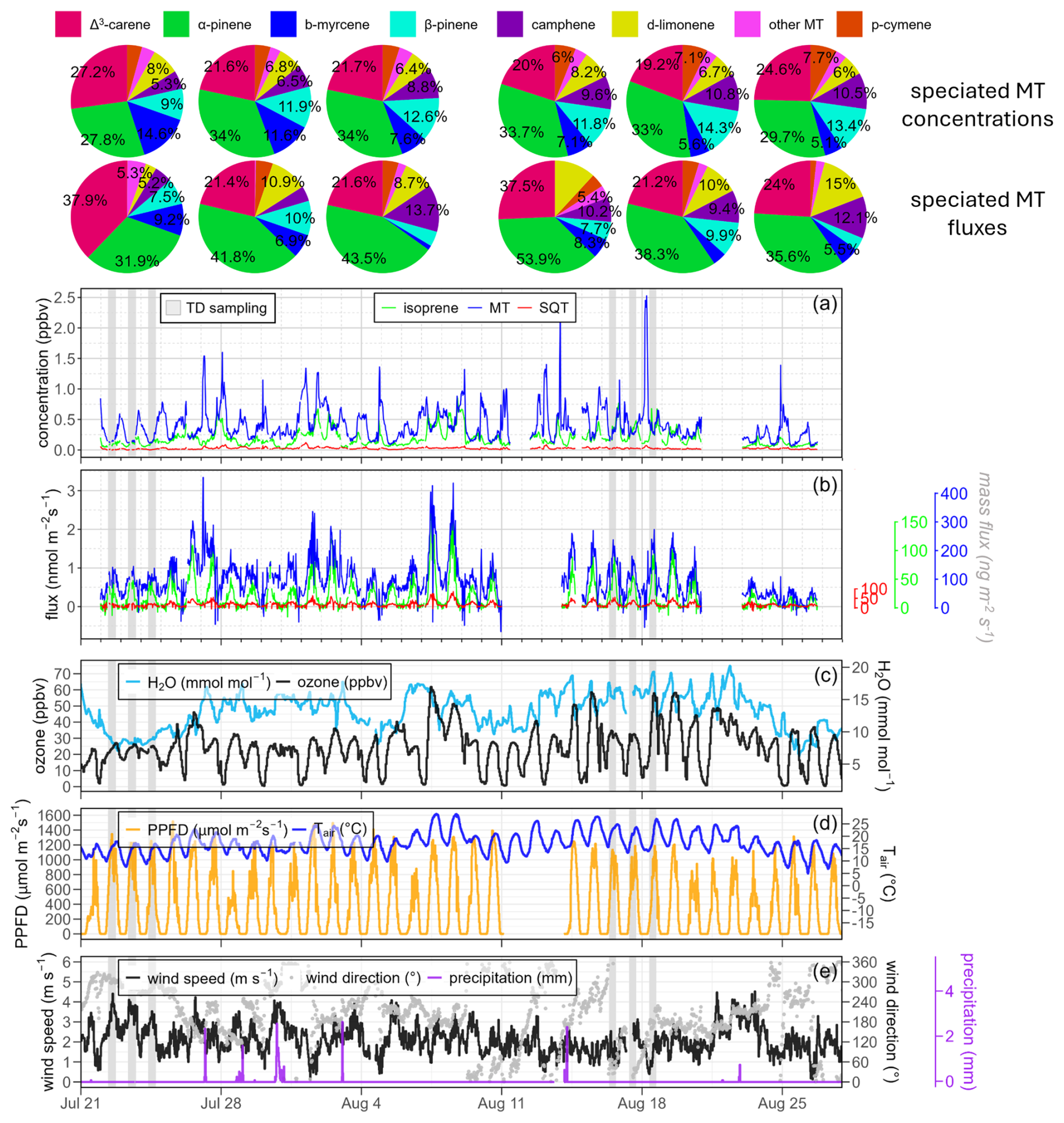
Figure 2 The 30 min BVOC concentrations (ppbv) and fluxes (nmol m⁻² s⁻¹) sampled at the 35 m BVOC inlet at ICOS Norunda, as well as related meteorological measurements. Shaded areas depict manual TD BVOC sampling periods at 37 and 60 m on the Norunda flux tower. The pie charts indicate the relative speciation of MT compound (top row) concentrations at 37 m and (bottom row) fluxes (via SLG flux method) as determined from the TD BVOC samples (percentages shown are >5 %). (a) MT, isoprene, and SQT concentrations (ppbv) and (b) EC-derived fluxes (nmol m⁻² s⁻¹) from the Vocus PTR-ToF-MS. The equivalent mass-flux (ng m⁻² s⁻¹) for isoprene, MT, and SQT is depicted along the right-hand y-axis. (c) Ozone concentration (ppbv) and water vapor (mmol mol⁻¹). (d) PPFD (µmol m⁻² s⁻¹; at height 55 m) and air temperature (°C; at 37 m). (e) wind speed (m s⁻¹), wind direction (°), and precipitation (mm). Set of displayed measurements span from 21 July to 27 August 2020.

3 Results

3.1 Meteorological and other conditions during campaign

Temperatures during the campaign varied between 13 and 22 °C. The typical prevailing wind direction was between south and northwest. Light precipitation occurred on manual sampling day 9 June. The meteorological conditions during the campaign EC measurements are displayed in Fig. 2. Typical peak daytime photosynthetic photon flux density (PPFD) varied from 700 to 1500 µmol m⁻² s⁻¹. Conditions during days when TD sampling was performed (8–10 June, 22–24 July, and 16–18 August) had consistent temperature (mean 17.4 ± 3.7 °C) and PPFD (mean 901 ± 319 µmol m⁻² s⁻¹) conditions. Ozone monitoring was available throughout the campaign from the nearby Norunda-Stenen station, via a Model E400 Teledyne ozone analyzer, located 1.4 km east of the Norunda tower. One interruption to Vocus sampling occurred on 12–13 August due to an electrical failure in the instrument shelter. A summary of the campaign time series is presented in Fig. 2, in which the campaign observations of the station water vapor, vapor pressure deficit (VPD), and dew point temperature are also included.

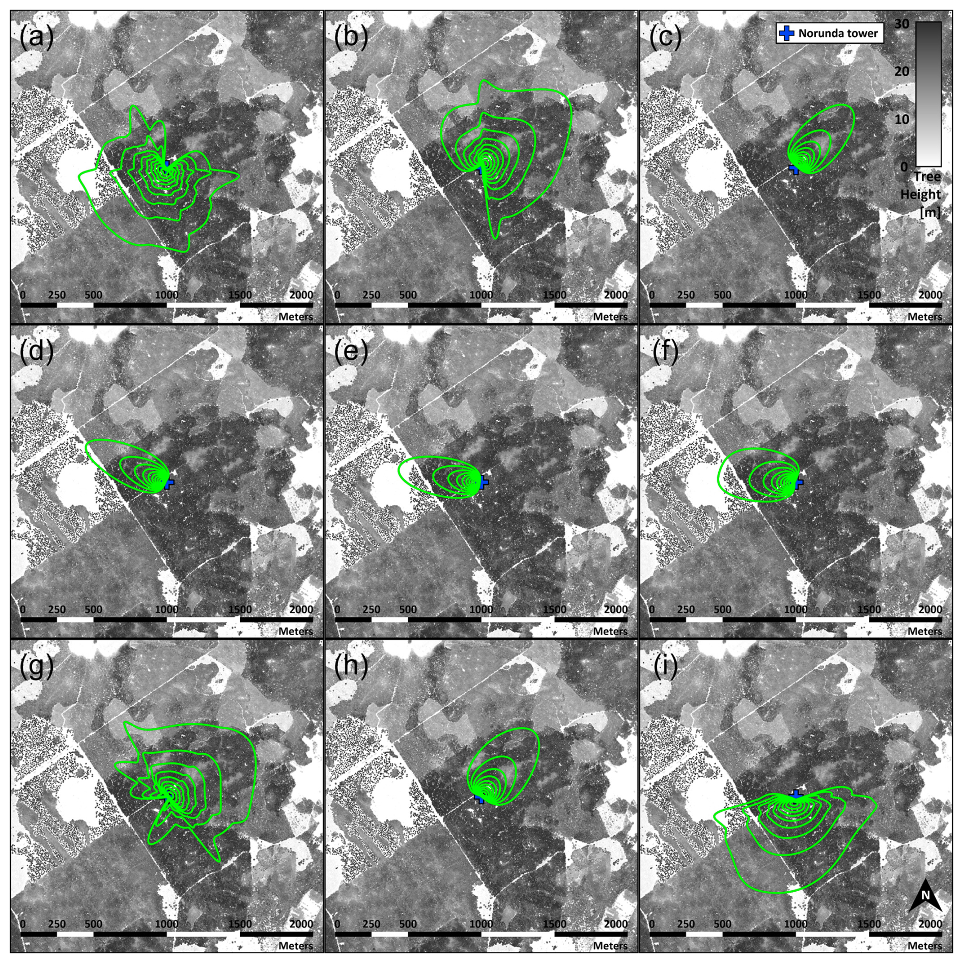
Figure 3 Daytime (from 09:00 to 17:00 CEST) average footprint estimates for SLG-derived fluxes using the two TD BVOC sampling heights (37 and 60 m) on the Norunda flux tower. Footprint contour lines (green) are shown in 10 % increments from 10 % to 90 %. Displayed footprints assessed at geometric-mean height (47.1 m) of TD sampling levels, following Horst (1999) for footprint estimation of SLG-method surface fluxes under unstable atmospheric stratification above-canopy (see Fig. 5f). The panels show these footprints for (a–c) 8, 9 and 10 June, (d–f) 22, 23, and 24 July and (g–f) 16, 17, and 18 August respectively.

3.2 Gradient sampling conditions during campaign

3.2.1 Sampling footprint comparison

To accurately interpret BVOC fluxes derived from concentration gradient measurements, it is important to assess the gradient-flux method footprint for the two TD sampling levels (37 and 60 m). A flux footprint analysis at their geometric-mean height (47.1 m), as suggested by Horst (1999) for two-height gradient-profile flux estimates, was conducted for each daily period corresponding to TD tube BVOC gradient sampling on the Norunda flux tower. Each footprint was calculated using the flux footprint model developed by Kljun et al. (2015). The Flux Footprint Prediction (FFP) model is a two-dimensional parameterization for the flux footprint based on a scaling approach to its crosswind distribution (e.g., Kljun et al., 2004, 2015). It was found that the footprints, particularly for ca. 85th percentile and below footprint contours (depicted in Fig. 3), in general compared well with each other in terms of the forest area and composition covered. Since the geometric-mean height for the SLG estimates is above the Vocus inlet height (35 m), the total extent of the estimated SLG footprints tended to be slightly larger than the EC flux footprint.

During the campaign TD measurements approximately 90 % of the flux measured by the Vocus tower inlet at the 35 m level originated within 350 m of the tower itself. For comparison, at 47.1 m, approximately 90 % of the observations originated from within 420 m of the tower.

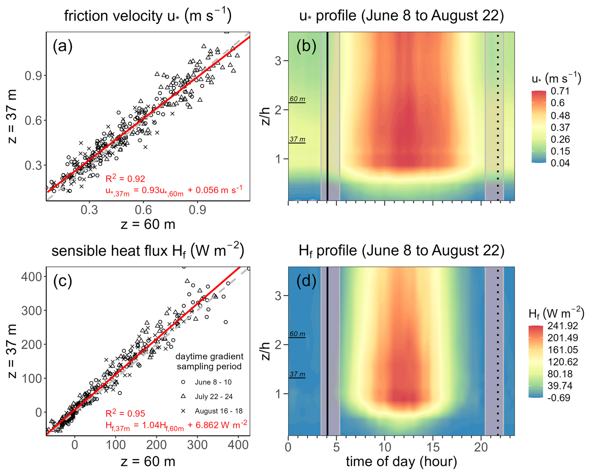
Figure 4 Comparison between friction velocity u_∗ (m s⁻¹) and sensible heat flux H_f (W m⁻²) measured at two heights above the forest canopy. (a, c) A best-fit comparison between 37 and 60 m for (a) friction velocity and (c) sensible heat flux during the 3 d sampling periods in June, July and August. The dashed line indicates a 1:1 relation, while the solid red line indicates the best fit linear regression. (b, d) Diurnal mean contour profiles for the 2020 Norunda campaign of (b) friction velocity u_∗ and (d) H_f with respect to the normalized height $z/h$ (canopy height h=28 m) in and above the Norunda forest. The relative heights of the 37 and 60 m sampling levels on the normalized height scale are indicated on the y-axis. In (b) and (d) panels, mean daily sunrise (solid vertical line) and sunset (dotted vertical line) are indicated. Shaded region indicates the range of sunrise and sunset times during the 9 June to 22 August campaign period.

3.2.2 Vertical micrometeorological conditions

An important prerequisite for the gradient-flux method is that vertical fluxes remain constant within the observation layer. To validate this constant-flux assumption, we compared the friction velocities, heat fluxes, and roughness lengths measured at both the 37 and 60 m measurement levels.

Measured sensible heat and momentum fluxes were similar at both measurement heights (see Fig. 4), with the mean linear fit of friction velocity and sensible heat flux between the 37 and 60 m heights being $u_{\ast ,\mathrm{37}\mathrm{m}}=\mathrm{0.93}{u}_{\ast ,\mathrm{37}\mathrm{m}}+\mathrm{0.056}\mathrm{m}{\mathrm{s}}^{-\mathrm{1}}$ and $H_{\mathrm{f},\mathrm{37}\mathrm{m}}=\mathrm{1.04}{H}_{\mathrm{f},\mathrm{60}\mathrm{m}}+\mathrm{6.9}\mathrm{W}{\mathrm{m}}^{-\mathrm{2}}$, respectively. Table C1 (see Appendix C) lists a summary of these friction velocity and sensible heat flux ratios under different stability conditions and wind directions. Atmospheric instability above canopy (i.e., Obukhov length $L^{-\mathrm{1}}<-\mathrm{1000}$; see Fig. 5f) prevailed during the times of daytime TD sampling. Stable atmospheric conditions were generally observed at night, while near-neutral conditions were typically observed during the transition in stability following sunrise and preceding sunset. It was found that, while near-neutral and stable conditions could lead to relatively large deviations in these ratios, for unstable atmospheric conditions the ratios were close to unity.

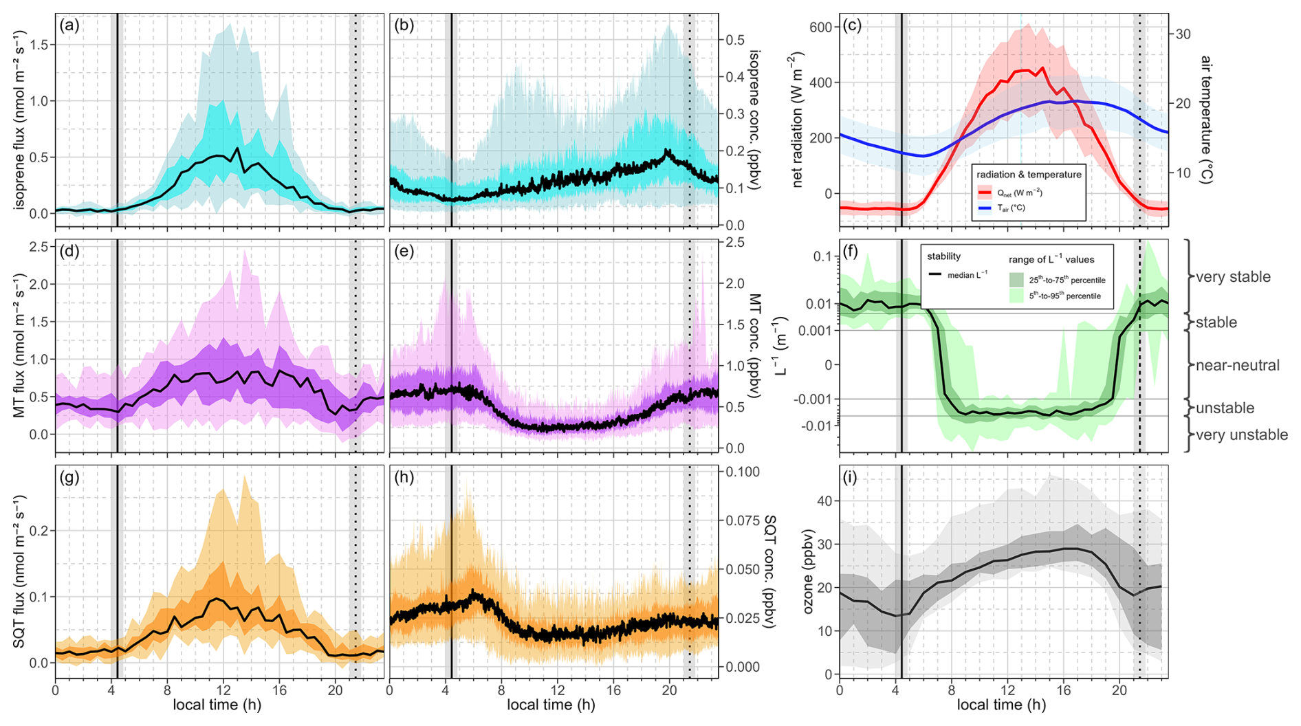
Figure 5 Diurnal range of fluxes and concentrations for (a, b) isoprene, (d, e) total MT, and (g, h) total SQT, as measured from the tower BVOC inlet using Vocus PTR-ToF-MS during the Norunda 2020 BVOC field campaign. Diurnal fluxes shown represent 30 min EC ensemble averages and diurnal concentrations represent 1 min averaged time series data. Shaded regions in panels indicate the 5th-to-95th and the 25th-to-75th quantile range, as well as the mean (solid line). (c) Net radiation (red) and canopy temperature (blue). Shaded regions for net radiation and temperature indicate one standard deviation. (f) Plot of the inverse of the Obukhov length (L⁻¹), indicating atmospheric stability above the canopy (measured at 36 m). (i) local diurnal ozone concentration (ppbv). In all the panels, mean sunrise and sunset (solid and dotted vertical lines, respectively) for the period of Vocus deployment (21 July 21 to 27 August) are indicated. Vertical bars (gray) indicate the range of sunrise and sunset times during this period.

3.3 Concentrations and fluxes of terpenes and other VOCs

During the campaign, the mean daytime isoprene concentration measured by the Vocus PTR-ToF-MS was 250 pptv. As shown in Fig. 2, the maximum concentration values occurred during daylight hours, at a time when temperature and PPFD were high (>20 °C and >1000 µmol m⁻² s⁻¹) as well, with concentrations falling to daily lows towards the evening. Little to no isoprene flux was observed at night. Peak total MT concentrations (1–1.4 ppbv) were typically significantly higher than isoprene concentrations. Unlike isoprene, peak total MT concentration typically occurred at night during stable atmospheric conditions in the canopy similarly to the observations by Petersen et al. (2023).

Such diurnal cycles in concentration were regularly observed throughout the campaign. Figure 5 shows the diurnal variation in isoprene, total MT, and total SQT from the Vocus PTR-ToF-MS measurements collected (21 July to 27 August) during the 2020 Norunda field campaign.

Isoprene had its highest concentrations above forest canopy during the day, with peaks typically in the morning between 07:00–11:00 CEST and more strongly between 16:00 CEST and sunset, whereas MT and SQT concentrations typically peaked at night. Isoprene and terpene fluxes, meanwhile, generally all peaked around noon. This diurnal concentration behavior by isoprene and total SQT, as was observed for total MT, was due to interplay of emission dynamics and the changes in atmospheric stability in the surface boundary layer. For isoprene, this was due to the light-dependent nature of emissions (i.e., de novo synthesis emissions (e.g., Guenther et al., 1995, 1993)), with emissions effectively shut down with the cessation of photosynthesis activity at night. On the other hand, the MT and SQT emissions of evergreen boreal tree species like Scots pine and Norway Spruce still have considerable nighttime emission from resin ducts and other tissue structures that are temperature-only-dependent (i.e., storage emission, rather than wholly de novo emission (e.g., Ghirardo et al., 2010; Guenther et al., 1995, 1993; Tingey et al., 1980)). It should also be noted that many SQTs have a short (∼0.1–10 s) chemical lifetime relative to MT, and that this is reflected in the observed concentrations measured by the Vocus, as a substantial fraction is expected to react with atmospheric radicals or other compounds before reaching the measurement height (e.g., Atkinson and Arey, 2003; Rinne et al., 2012). This diurnal behavior highlights the interplay between constitutive (non-stress induced) emissions, driven by environmental conditions (principally, photosynthetic light and temperature), and the atmospheric stability within the forest canopy. Despite lower emission rates of terpenes at night, as observed from their EC fluxes (see Fig. 5d and g), the stable nighttime atmosphere, as indicated by the Obukhov length (see Fig. 5f), causes a buildup in their concentrations at night. It was observed that terpene concentrations are typically greatest at or just following sunrise. Similar diurnal behavior was observed in other VOC compounds measured by the Vocus, such as acetone, acetaldehyde, and toluene, among others, and is also consistent with previous BVOC PTR-MS field campaigns at ICOS Norunda (Petersen et al., 2023). This diurnal terpene behavior is also consistent with observations at other boreal sites (e.g., Borsdorf et al., 2023; Hakola et al., 2012; Hellén et al., 2018).

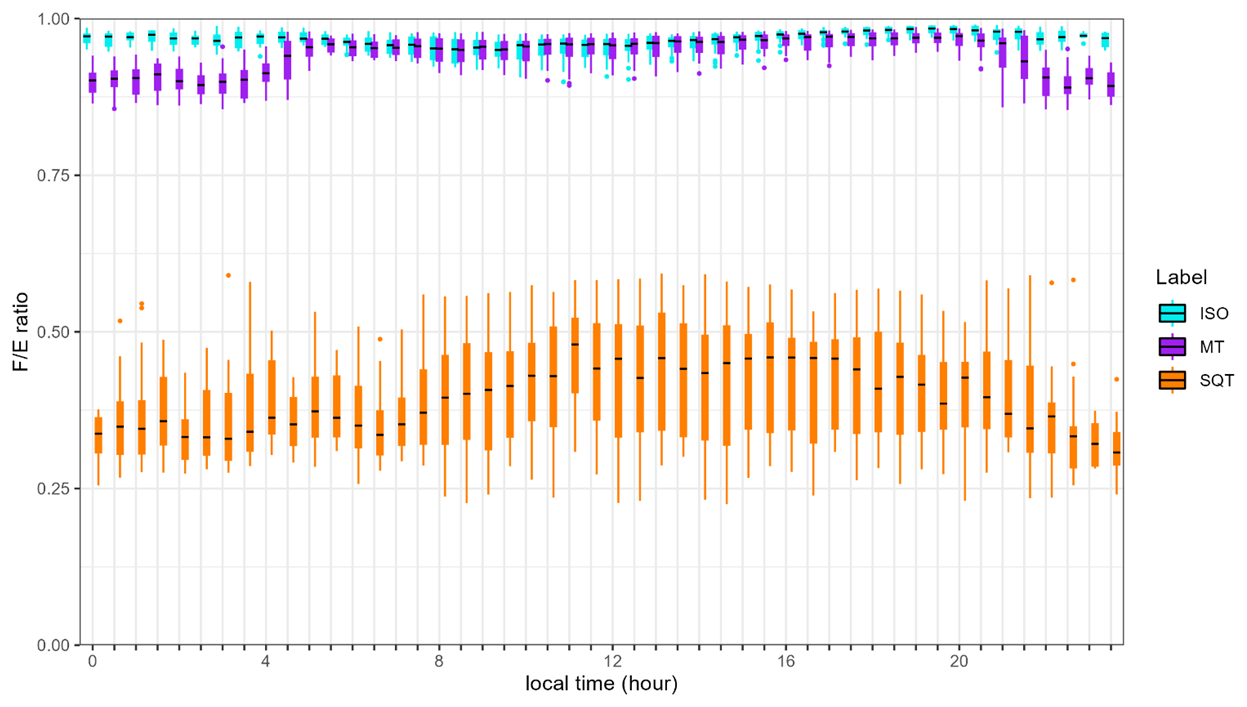
Figure 6 Boxplot of mean diurnal $F/E$ ratios for chemical degradation estimates of isoprene (cyan), MT (purple), and SQT (orange) for the 2020 Norunda BVOC campaign. Black dash of whisker plot indicates the median value.

3.3.1 Surface exchange rates

To quantify the actual SER of reactive VOCs, the effect of chemical degradation on the SER of isoprene, MT, and SQT was estimated. For ecosystem–atmosphere exchange, whereas above-canopy fluxes quantify the cumulative effect of within-canopy processes, including chemical degradation, the SER characterizes the net emission and deposition occurring at the ecosystem's soil and vegetation surfaces in the absence of this chemical sink. The effect of chemical degradation on the ratio of measured flux to SER, $R=F/E$, is shown in Fig. 6. Following the modeling work of Rinne et al. (2012) for a similar boreal forest, the $F/E$ ratios for MT are based on the reaction rate constants of α-pinene and for SQT on the reaction rate constants of β-caryophyllene. The effect of the chemical degradation rate of isoprene and MT, relative to the observed fluxes, was found to be minimal. The influence of chemical degradation on isoprene ($F/E=\mathrm{0.981}$ ± 0.013 at night and 0.957 ± 0.013 during day) was within the EC flux measurement uncertainty. The main influence of chemical degradation for total MT was found to be at night and, in terms of absolute emission increases, during peak flux periods around noon. For total MT, a daytime average of $F/E=\mathrm{0.957}$ ± 0.013 due to chemical degradation was calculated for daytime (within the uncertainty of EC flux measurements), while the nighttime loss was estimated at an average $F/E=$ 0.90 ± 0.03.

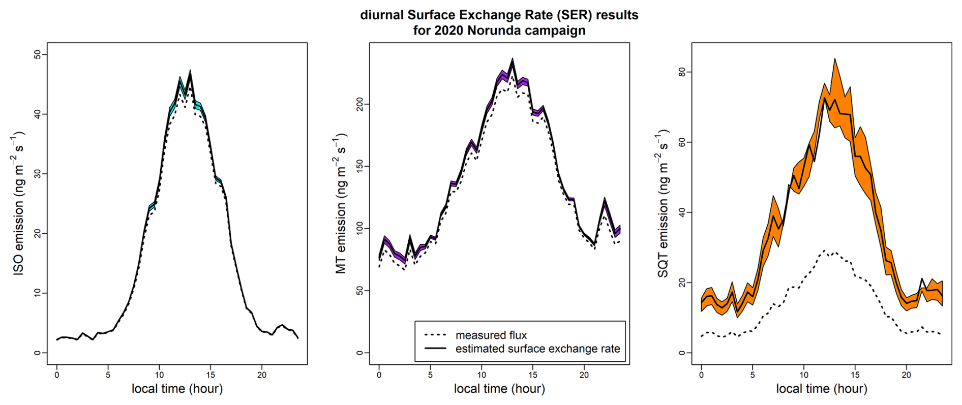
Figure 7 Mean diurnal SERs for isoprene, MT, and SQT during the 2020 Norunda campaign. Shaded region indicates the range of uncertainty for the modeled ozone, OH, and NO₃ reaction rate coefficients. Dashed black line indicates the corresponding measured flux.

In contrast, the measured SQT flux was significantly affected by chemical degradation (see Fig. 7). For the full campaign, the estimated SQT nighttime $F/E$ ratio is typically ca. 0.35 (varying from 0.31 to 0.41), while the daytime ratio is ca. 0.41 (varying from 0.37 to 0.47). The mean diurnal measured fluxes and inferred SERs of isoprene, MT, and SQT, for their respective OH, O₃, and NO₃ reaction rate constants (Table C3 in Appendix C), are shown in Fig. 7. As a consequence, for the diurnal average over the full campaign, peak SQT nighttime emission rates are typically ca. 240 % to 310 % (mean ca. 290 %) times greater, and SQT daytime emissions ca. 240 % to 290 % (mean ca. 260 %) times greater than would otherwise be inferred solely from EC flux measurements if the effect of chemical degradation on SQT exchange and subsequent SQT flux observations were neglected.

The effect of chemical degradation on the $F/E$ ratio between the TD sampling heights was also investigated. This was done to gauge an underpinning assumption of the SLG method: that there is no significant chemical sink between the sampling heights used to determine the above-canopy gradient. This was performed by evaluating, instead of $R=F/E$, the value of $R_{\mathrm{2}}/R_{\mathrm{1}}=F_{\mathrm{2}}/F_{\mathrm{1}}$, where R₁ and R₂ are the flux-to-emission ratios for the sampling heights z₁=37 m and z₂= 60 m, respectively. This provides a measure for the percent of flux lost between the lower and upper heights for the gradient measurement. For MT, there was typically only 1.7 (± 0.5) % flux loss between sampling heights, with $R_{\mathrm{2},\mathrm{MT}}/R_{\mathrm{1},\mathrm{MT}}=\mathrm{98.3}$ (varying from 97.8 to 98.8). This is less than the $F/E$ ratio previously found for the total MT EC flux measurements. In contrast, for SQT, there was typically between 33 % and 43 % loss in SQT flux between these heights, with $R_{\mathrm{2},\mathrm{SQT}}/R_{\mathrm{1},\mathrm{SQT}}=\mathrm{61.8}$ (varying from 57.1 to 66.6). As expected, this demonstrates significant SQT chemical loss between the two intervening heights, and that the SLG method would be inapplicable to SQT fluxes without significant modification to account for chemical degradation.

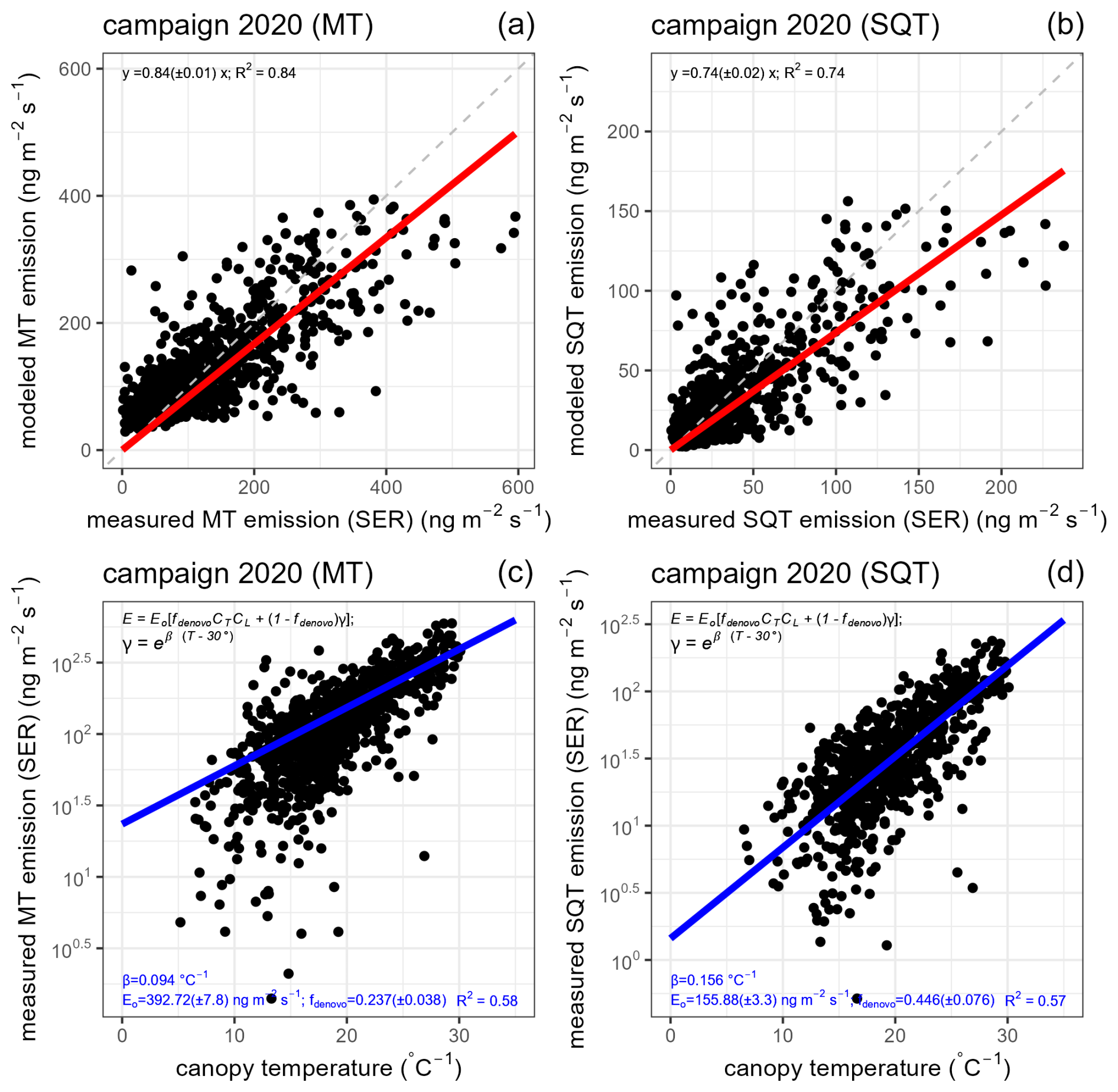
Figure 8 Hybrid emission algorithm comparison to terpene measurements. (a, b) Comparison of measured vs. modeled emission (using the fitted coefficients) for (a) MT and (b) SQT SERs. The red line indicates the linear regression best-fit line for the data points, and dashed gray line indicates the one-to-one line. (c, d) Plots of the canopy temperature vs. (c) MT emission and (d) SQT emission. Blue line shows the best-fit regression line.

3.3.2 Comparing measured terpenoid emissions with emission algorithms

The presented emission algorithm regression results (specifically, for the terpenes) are presented in Fig. 8. As the estimated isoprene SERs were within the range of uncertainty of the measured fluxes, only the measured isoprene fluxes were used for the regression analysis. For isoprene, we used the fixed β=0.09 °C⁻¹ of Guenther et al. (1993), and the emission algorithm was set to pure de novo synthesis emission by setting f_denovo to unity. The fitted isoprene E_o was found to be 85.0 (± 1.5) ng m⁻² s⁻¹.

For MT emissions based on the temperature-dependent pool emission algorithm (Guenther et al., 1993, 2012), by setting f_denovo to 0, the fitted MT standardized emission E_o was found to be 386 (± 5) ng m⁻² s⁻¹ for β=0.1 °C⁻¹ (Guenther et al., 2012). Allowing β to vary as a regression coefficient for the pool algorithm as well yields 370 (± 9) ng m⁻² s⁻¹ and β=0.094 (± 0.003) °C⁻¹. Applying the full hybrid MT emission algorithm, combining de novo synthesis and pool storage emission (e.g., Taipale et al., 2011), with the previously fitted β=0.094 °C⁻¹, yields E_o=374 (± 7) ng m⁻² s⁻¹, and the fraction of MT emissions originating from de novo synthesis as f_denovo=26 (± 4) %. When using the MT SERs instead of the observed EC fluxes at 37 m, fitting the hybrid algorithm then yields E_o=393 (± 8) ng m⁻² s⁻¹ and f_denovo=24 (± 4) %.

As the SQT emission rate is significantly under-represented by the measured flux due to chemical degradation, we fitted the hybrid emission algorithm to the estimated SQT SERs for the campaign. For fitting from SQT SERs, based on the temperature-dependent pool emission algorithm of Guenther et al. (1993, 2012), the fitted standardized SQT emission E_o was found to be 171 (± 3) ng m⁻² s⁻¹ for β=0.17 °C⁻¹ (Guenther et al., 2012). Allowing β to vary as a regression coefficient for the pool algorithm as well yields 160 (± 5) ng m⁻² s⁻¹ and β=0.156 (± 0.004) °C⁻¹. Applying the hybrid emission algorithm, combining de novo synthesis and pool storage emission (e.g., Taipale et al., 2011), with the previously fitted β=0.156 °C⁻¹, yields E_o=156 (± 3) ng m⁻² s⁻¹, and the fraction of SQT emissions originating from de novo synthesis as f_denovo=45 (± 8) %. Fitting the hybrid algorithm using the estimated SERs for SQT yielded better fits than simply applying the measured SQT flux data without the corresponding correction for chemical degradation. From the SERs, the hybrid algorithm estimates for f_denovo for both MT and SQT were found to be quite similar (38 (± 8) % and 31 (± 7) %, respectively).

3.3.3 Other VOCs

Acetaldehyde ($m/z+=\mathrm{45.034}$) exhibited a mean daily concentration of 0.7 ppbv. Concentrations of toluene ($m/z+=\mathrm{93.07}$) were generally low during daytime (∼12 pptv) and increased during nighttime (∼30 pptv), This behavior by toluene is consistent with the buildup of anthropogenic background emissions during night in the shallow nocturnal boundary layer (Karl et al., 2004). Similar behavior was found for the mass peak at $m/z+=\mathrm{95.049}$ (i.e., phenol), which had a concentration minimum during daytime (∼ 9 pptv) and maximum during nighttime (∼ 40 pptv). Acetic acid ($m/z+=\mathrm{61.028}$) was typically lowest after sunrise (∼ 10 pptv), gradually increasing throughout the day and peaking before sunset (∼ 33 pptv), then declining overnight. The exception to this trend occurred when high nighttime canopy concentrations coincided with similar peaks in acetone and acetaldehyde. The diurnal signal for $m/z+=\mathrm{41.039}$ and $m/z+=\mathrm{103.112}$, representing the PTR-protonated hexanol fragment and the hexanol parent ion, respectively, followed a similar pattern to acetone. The minimum in hexanol concentration (∼ 50 pptv) typically occurred in the morning following sunrise and peaked after sunset (∼ 130 pptv). Methyl vinyl ketone and methacrolein (MVK+MACR, $m/z+=\mathrm{71.049}$), two important intermediate products from the photochemical oxidation of isoprene, averaged 7 pptv daily.

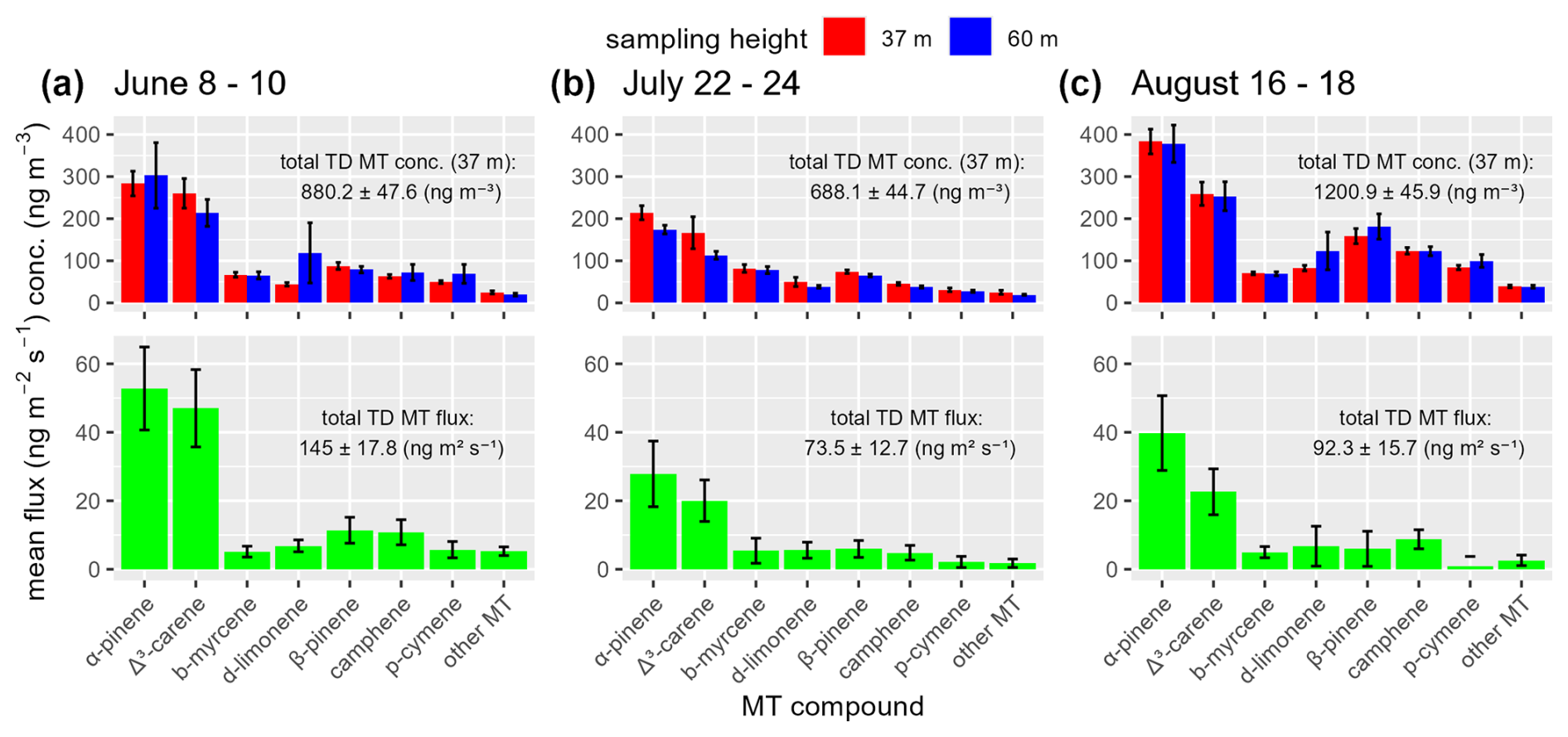
Figure 9 Monthly sampling-period mean concentrations of MT compound species at 37 (red) and 60 m (blue) on the station flux tower at the ICOS Norunda boreal forest, as well as sampling period mean speciated MT fluxes (green), during 8–10 June (a), 22–24 July (b) and 16–18 August (c). Vertical error bars indicate the standard mean error. The daily mean concentrations and fluxes are shown in Fig. C1 in Appendix C.

3.3.4 Speciated MT concentrations and fluxes

During the campaign, α-pinene, Δ³-carene, β-pinene, camphene, myrcene, and limonene were detected in the ATD-GC–MS analysis. The most abundant MT species throughout the campaign was α-pinene, followed by Δ³-carene (see Figs. 2 and 9). Limonene concentrations contributed approximately 5 %–10 % of total MT concentrations. An overview of the monthly sampling-period mean concentrations and SLG method-derived fluxes of the speciated MT compounds, observed via thermal desorption sampling at 35 m above the forest canopy, during the 3 d monthly sampling periods in June, July, and August is shown in Fig. 9. A daily mean evaluation can be found in the Appendix. During all sampling periods, α-pinene was the most prevalent MT compound present, fairly constant and typically representing between ca. 28 % to 34 % of the total MT concentration. The second most prevalent MT compound was Δ³-carene. From June to August, fraction of Δ³-carene among the MT compounds decreases by ca. 8 %, from monthly sampling-period averages of ca. 30 % in June, to ca. 24 % in July and ca. 22 % in August. During the June measurements, the typical concentration abundance at 37 m above the forest canopy among the MT species were 32 (± 4) % α-pinene, 30 (± 4) % Δ³-carene, 7.6 (± 0.8) % myrcene, 5 (± 0.6) % limonene, and 10 (± 1.1) % β-pinene, 7.2 (± 0.6) % camphene, and 5.6 (± 0.5) % cymene. In July, the typical abundances were 31 (± 3) % α-pinene, 24 (± 6) % Δ³-carene, 12 (± 2) % myrcene, 7(± 2) % limonene, and 10.8 (± 0.9) % β-pinene, 4.5 (± 0.7) % camphene, and 4.5 (± 0.7) % cymene. In August, the typical abundances were 32 (± 3) % α-pinene, 22 (± 2) % Δ³-carene, 5.9(± 0.4) % myrcene, 6.9 (± 0.6) % limonene, 13 (± 2) % β-pinene, 10.3 (± 0.8) % camphene, and 7 (± 0.5) % cymene.

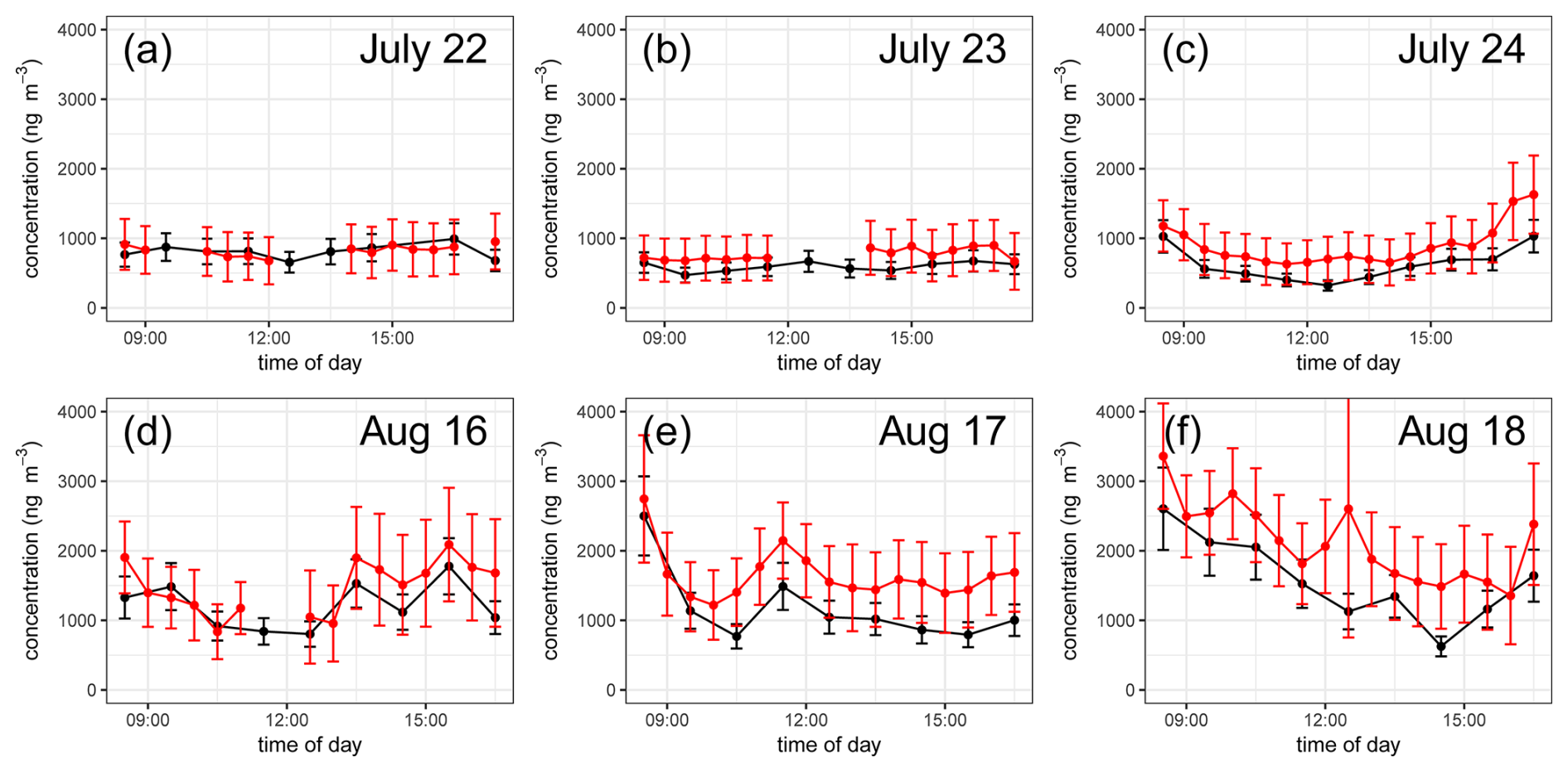
Figure 10 Comparison of MT concentration measurements from the Vocus PTR-ToF-MS (red) and the sum of speciated MT concentrations (black) from the TD sample GC-MS analysis. Summed TD MT displayed were measured at the 37 m TD sampling height. Error bars indicate (red) standard deviation of 30 min Vocus MT concentration and (black) uncertainty of summed TD MT concentrations based on the error analysis for TD sampling and analysis presented in Sect. 2.7. Shown are half-hourly time series of the MT concentration measurements from both Vocus and manual TD sampling for the (a–c) 22–24 July 2020 and (d–f) 16–18 August 2020 TD sample periods.

3.3.5 Vocus and ATD-GC-MS concentration comparison

We compared the sum of speciated MTs measured by GC–MS with the total MT concentration measured by Vocus PTR-ToF-MS. The comparison is displayed in Fig. 10. Based on comparison with 2022 precut TD measurements, it is expected that the sum of MT compounds identified by TD sample analysis represent 70 %–80 % of total atmospheric MT concentration. During 22–24 July the ATD-GC–MS obtained a concentration of 610 (± 30) ng m⁻³ while the Vocus measured 851 (± 27) ng m⁻³ for MTs. During 16–18 August, the ATD-GC–MS obtained a daytime concentration of 1201 (± 73) ng m⁻³ while the Vocus measured 1790 (± 73) ng m⁻³ for MTs.

3.4 Vocus EC flux results

During daytime sampling, the values of the Vocus MT flux typically ranged from 100 to 150 ng m⁻² s⁻¹ (see Figs. 2 and 5). Nighttime flux measurements should be treated with care, as stable atmospheric conditions during the evening lead to large uncertainties (e.g., Aubinet et al., 2012b). A combined estimate of the mean flux from the three-day sampling periods in June, July (start of Vocus campaign), and August (end of combined campaign) was performed for the SLG fluxes. The mean flux for each of these three-day sampling periods was calculated to reduce the large uncertainty in the SLG flux estimates, by reducing the influence of random errors in the calculation. For the period of 8–10 June gradient samples, the estimated mean summed MT flux was 108 (± 14) ng m⁻² s⁻¹. For the period of 22–24 July TD gradient samples, the estimated mean of the summed MT flux was 70 (± 20) ng m⁻² s⁻¹. For the period of 16–18 August TD gradient samples, the estimated mean summed MT flux was 90 (± 20) ng m⁻² s⁻¹. For comparison, during the 2020 campaign period when the Vocus was also operating, for the daytime sampling periods when TD sampling was performed the mean total MT flux from Vocus EC measurements for 22–24 July was 105 (± 3) ng m⁻² s⁻¹ and during 16–18 August was 155 (± 7) ng m⁻² s⁻¹. For these same periods, the estimated isoprene flux was 20 (± 9) ng m⁻² s⁻¹ and 23 (± 10) ng m⁻² s⁻¹, respectively.

To determine whether there were any significant changes in the relative mixture of speciated MT compounds emitted over the course of the 2020 campaign, a two-way analysis of variance statistical analysis was performed using the gradient-derived speciated MT fluxes. First, to eliminate the temperature-dependence of the MT emissions, the speciated fluxes were used to calculate temperature-normalized (to °C) emissions E₀ using the equation $E=E_{\mathrm{0}}\exp \left[\mathit{\beta }\left(T-\mathrm{30}\mathit{°}\mathrm{C}\right)\right]$ (Guenther et al., 1993), where E is the total MT emissions, β is an empirically fitted coefficient (found for the Norunda 2020 campaign to be β=0.094), and T is the temperature in °C. Next, for the two-way analysis of variance analysis, the flux data was sorted according to the monthly period (i.e., June, July, or August), and day of each sampling period (i.e., day 1, 2, or 3) when each gradient sample was collected. This allowed for the comparison of MT fluxes between sampling days and between sampling periods. The p-values from the analysis indicated that there was no significant (p<0.05) trend in the measured flux between the monthly sampling periods for the speciated MT compounds observed, with the exception of a weak negative trend in the emission of Δ³-carene when comparing the three monthly sampling periods, in particular, between June and August (p<0.0309). This indicates that at an ecosystem-scale level of emissions from the Norunda forest canopy, following from the gradient samples, at least during the summer months of June to August, no statistically significant variation was noted in the relative mixture of MT compounds emitted with respect to the time of season.

4 Discussion

We conducted a measurement campaign in a boreal forest in order to estimate speciated MT concentrations and fluxes during Scandinavian summer. The flux of MT compounds at Norunda was observed to primarily consist of α-pinene, followed by Δ³-carene (at approximately 60 %–70 % the rate of α-pinene). This is similar to the preponderance of α-pinene, followed by Δ³-carene, observed by Hakola et al. (2012) above the boreal forest at the Hyytiälä research station in Finland, a predominantly Scots pine forest with nearby Norway Spruce, as well. Speciated MT emissions showed no significant differences during summer-seasonal cycle. Only a slight weakening of the temperature-normalized emission rate for Δ³-carene was observed over the course of the 2020 measurements (June–August). It should be noted that observations did not extend to the spring and autumn, hence further attention to the seasonal behavior of individual MT species in BVOC emission and climate models may be warranted in future investigations.

These gradient-method flux measurements allow the speciated flux to be evaluated at an ecosystem-level scale, which sidesteps a potential issue for understanding ecosystem–atmosphere MT exchange, the large variability in speciated MT emissions that can exist among pine or spruce groups. Such variability, as observed in chamber measurement studies, can occur even among members of the same tree species and population (Bäck et al., 2012; Hakola et al., 2017).

The observed MT emissions were significantly temperature-dependent (fitting well to the storage-based pool emission algorithm of Guenther et al., 1993) and most of the forest MT emission originates from plant storage structures rather than from de novo synthesis as is the case for certain boreal tree species (e.g., Ghirardo et al., 2010). This is consistent with the forest tree species composition and the fact that MT mixing ratios were higher at night, with the lower boundary-layer height and stable atmosphere, despite that nighttime MT emission rates are lower (e.g., Rinne et al., 2009).

The influence of chemical degradation on the surface exchange rates of isoprene, MT, and SQT was also investigated. While the effect of chemical degradation on isoprene exchange rates was negligible (<5 %; less that EC flux uncertainties), a significant influence on the nighttime MT exchange rate was observed, with the exchange rate being on average ca. 10.8 % (varying from 6.8 % to 14.1 %) greater than measured MT flux. This was far more evident with the overall SQT exchange rates, which diurnally were on average ca. 160 % (varying 130 % to 180 %) greater during day and ca. 190 % (varying from 140 % to 230 %) greater during night than the measured SQT flux.

The effect of MT and SQT chemical speciation on inferred SER rates should also be noted. Since the various individual MT and SQT compounds react at different rates with OH, O₃, and NO₃, these differences in turn affect the total MT and SQT fluxes that are ultimately observed above canopy using Vocus PTR-ToF-MS. Conversely, the estimation of SER rates from total MT and total SQT flux observations is therefore dependent on the relative mixture of emitted compounds considered. For example, for Δ³-carene (the second most commonly observed MT compound during the 2020 Norunda campaign, following α-pinene) the reaction rates for the radicals OH, O₃, and NO₃ are $\mathrm{8.8}\times {\mathrm{10}}^{-\mathrm{11}}$, $\mathrm{3.7}\times {\mathrm{10}}^{-\mathrm{17}}$, and $\mathrm{9.1}\times {\mathrm{10}}^{-\mathrm{12}}$ cm³ molec.⁻¹ s⁻¹, respectively (Atkinson, 1997). When these values are implemented in our quantification of chemical degradation effects on the MT SER rates, in lieu of the reaction rate constants for α-pinene, it yields nighttime SER values that are ca. 12.6 % (varying 7.7 % to 16.9 %) greater than measured flux. This is an increase from the nighttime SER estimate based on the reaction rates of α-pinene of ca. 10.8 % (varying 6.8 % to 14.1 %) for this SER-to-flux comparison. Also present are MT compounds that are far more reactive than either α-pinene or Δ³-carene. For example, relative to individual MT compounds, it was observed that the combined concentration of b-myrcene and d-limonene was exceeded only by α-pinene and Δ³-carene. The OH, O₃, and NO₃ rate constants for β-myrcene are $\mathrm{2.2}\times {\mathrm{10}}^{-\mathrm{10}}$, $\mathrm{4.7}\times {\mathrm{10}}^{-\mathrm{16}}$, and $\mathrm{1.1}\times {\mathrm{10}}^{-\mathrm{11}}$ cm³ molec.⁻¹ s⁻¹, respectively, while for d-limonene they are $\mathrm{1.7}\times {\mathrm{10}}^{-\mathrm{10}}$, $\mathrm{2}\times {\mathrm{10}}^{-\mathrm{16}}$, and $\mathrm{1.22}\times {\mathrm{10}}^{-\mathrm{11}}$ cm³ molec.⁻¹ s⁻¹, respectively (Atkinson, 1997). When we substitute these reaction rate constants into our SER evaluation procedure, for our SER-to-flux comparison, we find for b-myrcene during nighttime ca. 24.6 % (varying from 16.7 % to 33.3 %) and during daytime ca. 17.5 % (varying from 13.1 % to 21.8 %). Meanwhile, for d-limonene, we find during nighttime ca. 19.3 % (varying from 12.7 % to 26.4 %) and during daytime ca. 10.8 % (varying from 7.9 % to 13.4 %). These values are ca. 2.4 and 1.8 times greater during nighttime, and ca. 3.8 and 2.3 times greater during daytime, for b-myrcene and d-limonene, respectively, than the corresponding increases found for α-pinene. For the average concentration apportionment, over the course of the 2020 Norunda campaign, of the identified MT compounds α-pinene, Δ³-carene, b-myrcene, d-limonene, β-pinene, and camphene, the mean values of their reactivities for OH, O₃, and NO₃ are $\mathrm{8.9}\times {\mathrm{10}}^{-\mathrm{11}}$, $\mathrm{9.79}\times {\mathrm{10}}^{-\mathrm{17}}$, and $\mathrm{6.83}\times {\mathrm{10}}^{-\mathrm{12}}$ cm³ molec.⁻¹ s⁻¹, respectively. When using these reaction rate constants instead of those of α-pinene for the MT SER evaluation, this yields a diurnal SER estimate for total MT that is very close (∼ Δ1 %) to the estimate formed using the OH, O₃, and NO₃ reactivities of α-pinene, with an nighttime increase in SER from the measured MT fluxes of 12 % (varying from 7.7 % to 15.7 %), and a daytime increase of 6.1 % (varying from 4.3 % to 7.8 %). This indicates that α-pinene likely acts as a good proxy for the mixture of MT emissions from this and similar boreal forests when attempting to infer the effect of chemical degradation on observed fluxes as collected using total MT measurement instruments such as PTR-ToF-MS.

For the speciated MT fluxes it has been observed that, despite the relatively large uncertainty involved with the speciated MT fluxes (compared to total MT EC flux measurements), the fraction of MT flux from the most common MT compound, α-pinene, is somewhat higher than the fraction of their concentration relative to the other MT compounds (see Figs. 2 and 10). This condition is also found in other studies (e.g., Rinne et al., 2000a). A potential explanation of this observation is the influence of chemical degradation, particularly with respect to more reactive compounds such as myrcene and d-limonene, during turbulent transport within and above canopy. Another potential influence on speciated MT flux vs. concentration observations is from transport from outside the flux tower footprint. The observed concentrations used for gradient measurements are the result of emissions, sinks, chemical transformation, and transport, whereas the observed fluxes reflect the emissions and sinks solely in the flux footprint of the tower.

5 Implications

A significant implication of this work is the role that seasonal changes can have on the speciation of MT compounds and subsequently their impact on air chemistry. BVOCs like MT influence the tropospheric ozone budget (Archibald et al., 2020). MTs also contribute to the formation and/or growth of atmospheric SOA due to the gas/particle partitioning of their reaction products in the troposphere. The structure of MTs has a significant role in their reactivity. For example, endocyclic MTs (e.g., limonene, α-pinene, and 3-carene) have a greater aerosol formation potential and tend to react faster than compounds with exocyclic double bonds (e.g., β-pinene and camphene). In addition, b-myrcene, an acyclic MT with three double-bonds, has a significant effect on the overall MT reactivity of MTs investigated by TD sampling, despite being at lower concentrations than many of the observed MT compounds. For example, in July, while less than 14 % of total MT concentration, b-myrcene made up more than half (52 %) of overall observed MT ozone reactivity. Fast-reacting MTs can represent a significant fraction of total reactivity even at low concentrations (e.g., Yee et al., 2018). Subsequently, even small seasonal changes in their concentration can represent large changes in the reactivity of the overall MT population emitted.

From July to August, the average of the OH, ozone, and NO₃ reaction rate coefficients for the observed MT mixture decreased. This was mainly driven by month-to-month trends in the relative abundance of 3-carene and b-myrcene. While overall reactivity of MT towards OH, ozone, and NO₃ increased from July to August, due to an increase in overall MT concentration, that increase is less than would be expected if changes in speciation were neglected, particularly for ozone (from July to August, for example, a 31 ± 18 % overestimate of ozone's MT reactivity). The relative average decrease in total oxidative capacity between July and August sampling periods amounts to 16 ± 10 %, when evaluated at the average ozone and OH concentrations investigated during the TD sampling periods. This is primarily due to the impact of speciation changes on ozone's oxidation capacity (∼ 24 ± 11 % decrease for ozone, vs. ∼ 10 ± 3 % decrease for OH). At night, when NO₃ can form (modeled at 1 pptv), and when average OH and ozone concentration are lower, this drop in total oxidative capacity was 12 ± 3 % (decrease for NO₃'s capacity was 8 ± 3 %). While this is within the uncertainty of modeled OH, ozone, and NO₃ concentrations utilized in our evaluation of chemical degradation, it is still a significant difference that warrants further attention when considering the effects of MTs on air chemistry at the ecosystem scale for boreal forests in BVOC emission modeling.

While not the main focus of this investigation, the impact on SQT speciation is also significant. For example, at the 37 m height used for TD sampling, the measured concentration of longifolene greatly exceeds that of α-humulene at a ratio of 80 %-to-20 %. However, the reactivity of α-humulene towards ozone is more than 2.3×10⁴ times greater than that of longifolene. An approximate calculation using the same chemical degradation evaluation presented in this investigation indicates the converse for the speciation of these SQT emissions, indicating that α-humulene emission dominates that of longifolene at a ratio of nearly 90 %-to-10 %. As can be seen, this presents a useful potential tool for investigating the ecosystem-scale speciation of SQT emissions.

Another potential implication is the determination of SQT SERs at the ecosystem scale using a combination of measured fluxes and modeled F/E ratio. The breakdown of SQT has long been a limiting factor in evaluating surface emissions based on observed fluxes (e.g., Duhl et al., 2008; Helmig et al., 2006; Pollmann et al., 2005). The determination of the effect of chemical degradation on the surface exchange of reactive BVOC fluxes can be evaluated using measurements of ozone and the radicals OH and NO₃. While OH measurements have classically been difficult to conduct (e.g., Heard, 2006; Heard and Pilling, 2003; Stone et al., 2012), many stations regularly monitor ozone, often the leading contributor (by an order of magnitude (see Fig. B1)) to the SQT chemical degradation that attenuates observed SQT fluxes. In parallel with GC-MS or more recent tools such as ultrafast GC (e.g., Materiæ et al., 2015) for determining SQT speciation at the PTR EC inlet height, combining PTR-ToF-MS EC flux observations with chemical degradation analysis offers a promising avenue for evaluating ecosystem-scale SERs of SQTs and other highly reactive BVOC compounds.

Appendix A: Determination of displacement height d and the Γ correction factor

The displacement height d was determined using the velocity u and friction velocity u_∗ data from the vertical profile of sonic anemometers on the Norunda flux tower, using the approach described in Mölder et al. (1999), as well as with the empirical relation d=0.86 h found therein (where h is canopy height). The u and u_∗ data were filtered according to the selection criteria: $u\left(\mathrm{87}\mathrm{m}\right)-u\left(\mathrm{44}\mathrm{m}\right)>\mathrm{0.2}{\mathrm{m}\mathrm{s}}^{-\mathrm{1}}$ and $u_{\ast }>\mathrm{0.1}{\mathrm{m}\mathrm{s}}^{-\mathrm{1}}$. Good agreement for the displacement height d was found for d=24 m.

To correct the SLG flux measurements of speciated MT flux for the influence of the RSL above canopy, the Γ correction factor was determined by integrating the profile for γ(z) above the canopy (and within the RSL) from the lower TD sampling height (37 m) to upper sampling height (60 m).

The γ-coefficients above the canopy were calculated from the sensible heat flux H, temperature T, and friction velocity u_∗ from the sonic anemometer profile according to $\mathit{\gamma }={\mathrm{\Phi }}_h^{\mathrm{MO}}\left(\mathit{\zeta }\right)/{\mathrm{\Phi }}_h^{\mathrm{meas}}\left(z\right)$, where ${\mathrm{\Phi }}_h^{\mathrm{MO}}$ is the dimensionless gradient for sensible heat according to Monin–Obukhov similarity theory (where ζ is the stability parameter $(z-d)/L$), ${\mathrm{\Phi }}_h^{\mathrm{meas}}\left(z\right)$ is the dimensionless gradient for sensible heat according to measurements on the flux tower, k is the von Kármán constant, ρ is the density of air, and c_p is the specific heat capacity of dry air. To minimize errors in the derivative of θ(z) when calculating ${\mathrm{\Phi }}_h^{\mathrm{meas}}\left(z\right)$, the gradient $\mathrm{d}\mathit{\theta }/\mathrm{d}z$ was determined by fitting the profile sonic data for potential temperature θ(z) using the equation $\mathit{\theta }=a+b\ln \left(z\right)+c{\ln }^{\mathrm{2}}\left(z\right)$ (e.g., Mölder et al., 1999).

Measured γ values during the TD sampling periods on 8–10 June, 22–24 July, and 16–18 August, between 09:30 to 17:00 CEST, were collected. This vertical γ-profile above forest canopy was then used to fit the coefficients for a continuous profile for γ(z). We applied the following formula:

$$\begin{array}{}\text{(A1)}& \mathit{\gamma }\cong \mathrm{1}+A{e}^{-B(z-d)},\end{array}$$

where A and B are undetermined coefficients. This fitting formula derives from consideration of Garratt (1980) and Harman and Finnigan (2007). Following nonlinear regression, the fitted coefficients were found to be A=5.26 and B=0.12 (ΔA=1.01, ΔB=0.02). A plot of the vertical γ-coefficient profile between the TD sampling levels at z₁=37 and z₂=60 m during the 2020 Norunda campaign is shown in Fig. A1 (the fitted curve for Eq. (A1) appears in blue).

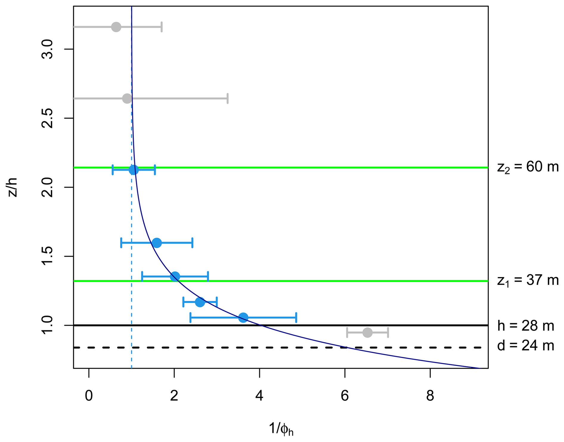
Figure A1 Vertical profile of γ above the Norunda forest canopy during daytime TD sampling. The x-axis shows the value of $\mathit{\gamma }=\mathrm{1}/{\mathit{\varphi }}_h={\mathrm{\Phi }}_h^{\mathrm{MO}}\left(\mathit{\zeta }\right)/{\mathrm{\Phi }}_h^{\mathrm{meas}}$, and the y axis shows the normalized height $z/h$. Points indicate median γ (± standard error of median) measured from ${\mathrm{\Phi }}_h^{\mathrm{MO}}\left(\mathit{\zeta }\right)/{\mathrm{\Phi }}_h^{\mathrm{meas}}$ during for the TD sampling periods (09:30 to 16:30 CEST; 8–10 June, 22–24 July, and 16–18 August 2024). Blue points (near or within RSL) indicate y used to fit function for the RSL layer. Dark blue curve indicates regression fit of $\mathit{\gamma }=\mathrm{1}+A{e}^{-B(z-d)}$ to the measured γ-profile values (A=5.26, B=0.12). Vertical dashed line indicates γ=1. Horizontal lines indicate (dashed black) displacement height d, (solid black) canopy height h, and (green) the z₁=37 m and z₂=60 m TD sampling heights.

Using z₁=37, z₂=60, d=24 m, and fitted coefficients $A=-\mathrm{5.26}$ and B=0.12, the integral of equation A1 was then used to determine a mean enhancement factor $\mathrm{\Gamma }=\frac{\mathrm{1}}{z_{\mathrm{2}}-z_{\mathrm{1}}}{\int }_{z_{\mathrm{1}}}^{z_{\mathrm{2}}}\mathit{\gamma }\left(z\right)\mathrm{d}z$. For the Norunda 2020 SLG flux measurements, this yielded $\mathrm{\Gamma }=\mathrm{1.36}\pm \mathrm{0.09}$.

$$\begin{array}{}\text{(A2)}& \begin{array}{rl}\mathrm{\Gamma }& \left(z_{\mathrm{1}}=\mathrm{37}\mathrm{m},z_{\mathrm{2}}=\mathrm{60}\mathrm{m}\right)={\displaystyle \frac{\mathrm{1}}{z_{\mathrm{2}}-z_{\mathrm{1}}}}\underset{z_{\mathrm{1}}}{\overset{z_{\mathrm{2}}}{\int }}\mathit{\gamma }\left(z\right)\mathrm{d}z\\ & ={\displaystyle \frac{A}{B}}\left[{\displaystyle \frac{e^{-B(z_{\mathrm{2}}-d)}-e^{-B(z_{\mathrm{1}}-d)}}{z_{\mathrm{2}}-z_{\mathrm{1}}}}\right]+\mathrm{1}\cong \mathrm{1.36}.\end{array}\end{array}$$

The uncertainty of this fitted estimate was determined using the standard errors of coefficients A and B, and propagation of uncertainty $\mathrm{\Delta }\mathrm{\Gamma }=\sqrt{{\left(\frac{\partial \mathrm{\Gamma }}{\partial \mathrm{A}}\mathrm{\Delta }\mathrm{A}\right)}^{\mathrm{2}}+{\left(\frac{\partial \mathrm{\Gamma }}{\partial \mathrm{B}}\mathrm{\Delta }\mathrm{B}\right)}^{\mathrm{2}}}\cong \mathrm{0.09}$.

Appendix B: Effect of chemical degradation on isoprene, MT, and SQT surface exchange rates

B1 Model calculations

The effect of chemical degradation on isoprene, MT, and SQT SERs was explored using the modeling supplement of Rinne et al. (2012), which made use of a stochastic Lagrangian transport chemistry model, and by parameterizing the reaction rates for ozone, OH, and NO₃, to estimate the SERs for the 2020 Norunda campaign's terpenoid EC flux dataset.

The effect of chemical degradation on measured fluxes of reactive compounds is closely related to the ratio the mixing time scale τ_t to the compound's chemical time scale τ_c, also known as the Damköhler number Da (Damköhler 1940), which can be written as

$$\begin{array}{}\text{(B1)}& Da={\displaystyle \frac{{\mathit{\tau }}_{\mathrm{t}}}{{\mathit{\tau }}_{\mathrm{c}}}}.\end{array}$$

In the case of Da≪1, the flux at the measurement height closely corresponds to the emission rate. For relatively large Da values, however, the compound will be affected by chemical degradation before reaching the measurement height, and the observed flux will be lower than the primary emission.

To estimate the flux-to-emission ratio ($F/E$) from measured Da-number ratios, lookup tables were used from the supplementary materials provided by Rinne et al. 2012. These tables relate the canopy-top Damköhler number (Da_h) to the flux-to-emission ratio ($F/E$) for specific normalized heights $z/h$ above the forest canopy-top height h. In this model, the LAI of the canopy, modeled according to the typical profile of a Scots pine forest, is 3.5. For comparison, LAI at Norunda is 3.6 (± 0.4) m² m⁻² (Petersen et al., 2023). Using an approximation for the mixing time scale of ${\mathit{\tau }}_{\mathrm{t}}=z/u_{\ast }$, the canopy-top Damköhler number (Da_h) was calculated using the relation

$$\begin{array}{}\text{(B2)}& D{a}_h={\displaystyle \frac{h}{u_{\ast }{\mathit{\tau }}_{\mathrm{c}}}},\end{array}$$

where the friction velocity u_∗ was measured at 37 m on the station flux tower (see example station BVOC inlet setup in Fig. 1 of the main text), h is the canopy height (28 m), and τ_c is the chemical lifetime of a given BVOC compound. The chemical lifetime τ_c can be calculated as

$$\begin{array}{}\text{(B3)}& {\mathit{\tau }}_{\mathrm{c}}={\left(k_{X,\mathrm{OH}}\left[\mathrm{OH}\right]+k_{X,{\mathrm{O}}_{\mathrm{3}}}\left[{\mathrm{O}}_{\mathrm{3}}\right]+k_{X,{\mathrm{NO}}_{\mathrm{3}}}\left[{\mathrm{NO}}_{\mathrm{3}}\right]+k_{X,\mathrm{photolysis}}\right)}^{-\mathrm{1}},\end{array}$$

where [OH], [O₃], and [NO₃] are the concentrations of OH, O₃, and NO₃, respectively, and where k_X,OH, $k_{X,{\mathrm{O}}_{\mathrm{3}}}$, and $k_{X,{\mathrm{NO}}_{\mathrm{3}}}$ are the reaction rate constants between the compound of interest X (i.e., isoprene, MT, SQT, etc.) and the radicals OH, O₃, and NO₃, respectively. Finally, k_{X, photolysis} is the photolysis rate of compound X. As k_{X, photolysis} for isoprene, MT, and SQT is much less than the rate of reactions with radicals OH, O₃, and NO₃, as in Rinne et al. (2012), it is dropped from subsequent calculations.

The reaction rate constants for isoprene, α-pinene and β-caryophyllene with respect to OH, O₃, and NO₃ used for the Norunda 2020 campaign SER analysis are listed in Table C3.

For the 2020 Norunda campaign SER analysis, modeling of the diurnal cycle of OH and NO₃, as well as local ozone data from the nearby Norunda-Stenen monitoring site, were used to calculate the time series of τ_c for isoprene, MT, and SQT, to then calculate Da_h for applying the Rinne et al. (2012) $F/E$ lookup tables.

The radicals OH and NO₃ were diurnally simulated for the Da_h calculations. The modeling choices for OH and NO₃ were informed by the HUMPPA-COPEC-2010 measurement campaign in Hyytiälä, Finland, and the settings implemented in Rinne et al. (2012). The OH concentration was assumed to vary diurnally between 0.3 × 10⁶ and 1.2 × 10⁶ molecules cm⁻³ over a Gaussian peak profile (t_mean= 12:00 CEST, σ_t=3.5 h). The uncertainty ΔOH was assumed to be 40 % of concentration.

NO₃ was assumed to vary as a step function, with a daytime concentration of zero and a nighttime concentration of 2.5 × 10⁷ molecules cm⁻³ (1 pptv), consistent with the breakdown of NO₃ under direct sunlight. The NO₃ concentration was assumed to linearly ramp between daytime and nighttime values during a 30 min widow before the daily sunrise and after daily sunset. The uncertainty ΔNO₃ was assumed to be 50 % of concentration.

The ozone data used for the τ_c-calculations came from the Norunda-Stenen monitoring station (1.4 km east of Norunda flux tower). To accurately reflect above-canopy nighttime concentrations, as model ozone data was collected well below canopy height, a nighttime minimum concentration was set at 5 × 10¹¹ molec. cm⁻³ (ca. 20 s ppbv). This conforms with previous campaign studies of the diurnal vertical ozone profile within and above the Norunda forest summer canopy (Petersen et al., 2023), where a significant nighttime sink was observed below canopy height (28 m). The uncertainty ΔO₃ was assumed to be 25 % of concentration.

The diurnal mean reaction rates of ozone, OH, and NO₃ with isoprene, as well as with α-pinene and β-caryophyllene (used as examples for MT and SQT, respectively), are shown in Fig. B1.

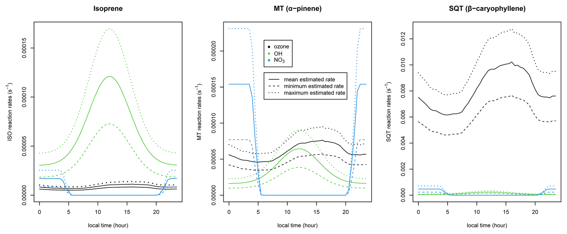
Figure B1 Diurnal mean reaction rates of ozone (black), OH (green), and NO₃ (blue) for isoprene, MT (α-pinene) and SQT (β-caryophyllene). Lines indicate the mean (solid) reaction rates, as well as the minimum (dashed) and maximum (dotted) -estimated values of the reaction rates based on the concentrations of OH, O₃, and NO₃ as well as the uncertainties ΔOH, ΔO₃, and ΔNO₃.

For the estimate of $F/E$ from Da_h, the lookup tables were used from the supplementary materials provided by Rinne et al. (2012). These tables relate the canopy-top Damköhler number (Da_h) to the flux-to-emission ratio ($F/E$) for specific normalized heights z/h above the forest canopy-top height h. In this model, the LAI of the canopy, modeled according to the typical profile of a Scots pine forest, is 3.5.

The $F/E$ modeling also includes the output for different parameterizations, such as canopy-source emission vs. ground-source emission, as well as the relative scaling of oxidation rates above vs. below-canopy. Several examples of the estimated diurnal $F/E$ ratios for the 2020 Norunda campaign under these different parameterizations are shown below (Fig. B2).

The ground source, for example, is likely appropriate for certain types of forest floor SQT emission (e.g., Mäki et al., 2019). In addition, daytime mixing may lead to equal or similar oxidation levels above and below canopy, as the canopy is well-mixed, while nighttime oxidation rates can become very stratified within stable canopy air, as was frequently observed for vertical profile of ozone within the Norunda canopy at night (see Fig. 7 therein). For the SER estimates presented in the main text, the source is modeled as being in the canopy, and the relative oxidation rates above and below canopy are modeled as being equal. For SQT (and for predominantly a canopy source), this can be addressed by interpolating between table lookup_C_o025.txt (i.e., nighttime stratified ozone) and table lookup_C_o100.txt (i.e., daytime well-mixed ozone), both found in the supplementary materials of Rinne et al. (2012), using the Monin–Obukhov atmosphere stability length L.

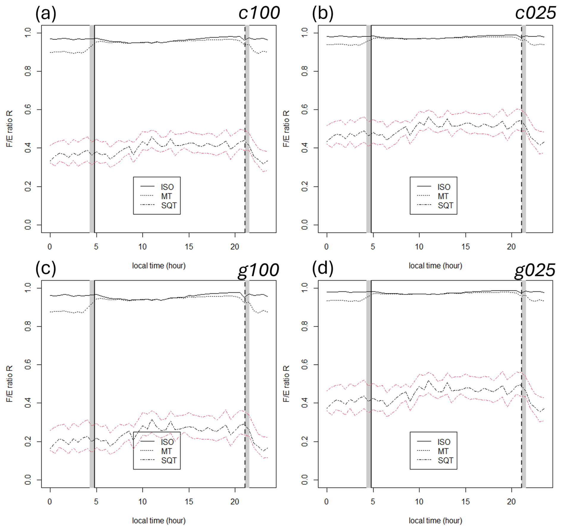
Figure B2 Diurnal $F/E$ ratios for isoprene, MT (α-pinene) and SQT (β-caryophyllene) for a range of different model parameterizations. (a, b) parameterized for canopy source. (c, d) parameterized for ground source. (a, c) below-canopy oxidation rate equals that of above-canopy. (b, d) below-canopy oxidation rate 0.25× that of above-canopy. The estimated $F/E$ ratios for the minimum and maximum of the ozone, OH, and NO₃ reactions rates are shown as dashed red lines.

B2 Impact of chemical speciation on estimated surface exchange rate uncertainty

Having described an approach for inferring SERs from measured fluxes, we now aim to investigate the conditions when applying a proxy or group-average estimate for the R ratio is justified when estimating emission rates from chemically degraded flux measurements of total SQT and nighttime total MT by PTR-MS instrumentation. Using the ratio $R=F/E$ (described in Sect. 2.8), we can write the total SQT flux measured by the Vocus PTR-ToF-MS as $F=\sum _i{F}_i=\sum _i{E}_i{R}_i=E\sum _i{\mathit{\chi }}_i{R}_i$, where χ_i is the fraction $E_i/E$ that each compound of the total mixture contributes to the total emission (with $\sum _i{\mathit{\chi }}_i=\mathrm{1}$). We can then define an effective R ratio for describing the total mixture as $R_{\mathrm{true}}=\sum _i{\mathit{\chi }}_i{R}_i$, an emission-weighted average of the compound-specific R values for all compounds contributing to the total group emission rate. In practice, even for the relatively well-behaved MT mixture, our knowledge of χ_i is limited. For estimating the SER it can, instead, be useful to use an estimate for R based on a compound commonly observed to dominate total emissions of a terpenoid group such as MT or SQT or, alternatively, use an estimate for the approximate emission rates based on previous chamber emission measurements at the surrounding site. The true and estimated total emission are $E_{\mathrm{true}}=F/R_{\mathrm{true}}$ and $E_{\mathrm{est}}=F/R_{\mathrm{est}}$, where R_est is the assumed group average or compound-specific proxy used for estimating the total emission rate. The relative error in the estimated total emission rate is $\mathit{ϵ}=\left|E_{\mathrm{est}}-E_{\mathrm{true}}\right|/E_{\mathrm{true}}=\left|\frac{\mathrm{1}}{R_{\mathrm{avg}}}-\frac{\mathrm{1}}{R_{\mathrm{true}}}\right|/\left(\frac{\mathrm{1}}{R_{\mathrm{true}}}\right)$, which simplifies to

$$\begin{array}{}\text{(B4)}& \mathit{ϵ}=\left|R_{\mathrm{true}}-R_{\mathrm{est}}\right|/R_{\mathrm{est}}.\end{array}$$

We proceed from here to estimate the impact that individual compounds in the mixture might have on the estimated total emission rate. While R_true might be elusive in practice, we can test the influence of individual compounds against an idealized case. For a test case where we can specify the emitted proportions, and in the case that the estimate for R is based on a single compound, Eq. (B4) simplifies to

$$\begin{array}{}\text{(B5)}& \begin{array}{rl}& \left|{\displaystyle \frac{R_{\mathrm{mix}}-R_k}{R_k}}\right|=\left|{\displaystyle \frac{\left(\sum _i{\mathit{\chi }}_i{R}_i\right)-R_k}{R_k}}\right|\\ & =\left|{\displaystyle \frac{\left(\sum _{i\ne k}{\mathit{\chi }}_i{R}_i\right)-(\mathrm{1}-{\mathit{\chi }}_k)R_k}{R_k}}\right|\\ & =\left|{\displaystyle \frac{\left(\sum _{i\ne k}{\mathit{\chi }}_i{R}_i\right)-\left(\sum _{i\ne k}{\mathit{\chi }}_i\right)R_k}{R_k}}\right|=\left|\sum _{i\ne k}{\mathit{\chi }}_i{\displaystyle \frac{R_i-R_k}{R_k}}\right|,\end{array}\end{array}$$

where χ_k and R_k=R_est are the emitted proportion and R ratio, respectively, of the proxy compound used for estimating the total SER, and R_mix is the weighted average of the R ratio based on the specified emitted proportions of the test case mixture. We can apply Eq. (B5) to a simple test based on three compounds.

For this three-compound test, we assume that the SQT mixture is similar to that observed in chamber emission measurements at Norunda in July and August 2014 (e.g., Wang et al., 2018) and at a similar boreal forest by Hellén et al. (2018). A summary of the compounds, proportions, and calculated R ratios are listed in Table B1. Based on observations, the proportion of longifolene is likely much lower (<1 %). From Kim et al. (2011), for an air temperature of 298 K and at sea-level pressure, we calculate the reaction rate coefficients for β-farnesene to be $k_{\mathrm{OH}}=\mathrm{2.9}\times$ 10⁻¹⁶ cm³ molec.⁻¹ s⁻¹ and $k_{\mathrm{ozone}}=\mathrm{6.9}\times$ 10⁻¹⁶ cm³ molec.⁻¹ s⁻¹. For the daytime OH and ozone concentrations listed in Table C3, the chemical lifetime of β-farnesene during the day is ca. 16 min.

Table B1 The proportions χ_i and calculated flux to surface exchange ratios R_i for the three compounds (β-caryophyllene, longifolene, and β-farnesene) used in the three-compound test case example.

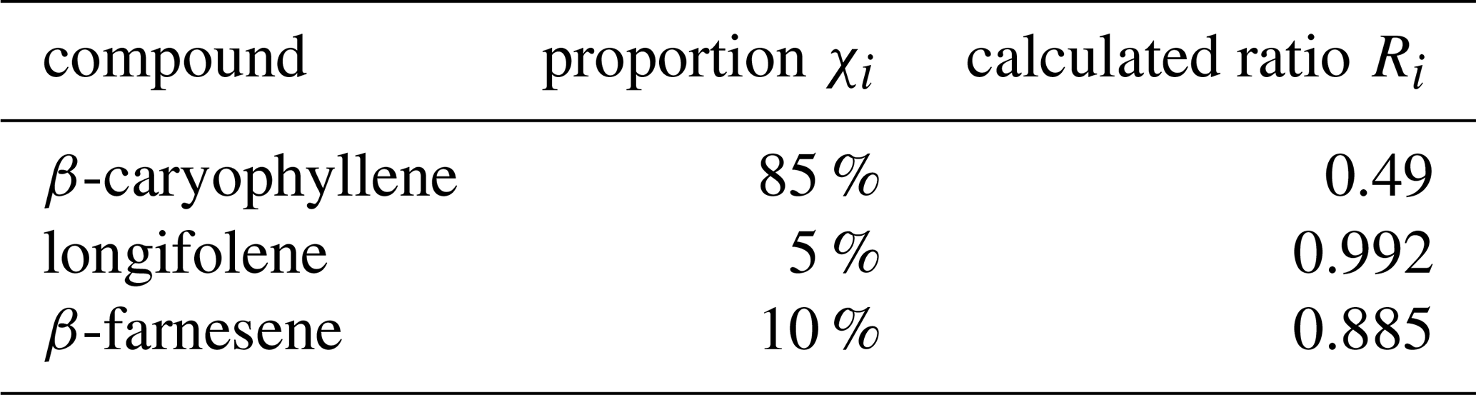
Applying this to Eq. (B5), we find that applying β-caryophyllene as a proxy leads to an offset of approximately 13 %. In comparison, the influence of uncertainty from modeled concentrations of daytime OH (± 40 %) and ozone (± 25 %) on the calculated SERs from the chemical degradation analysis 12 %) is approximately the same.

In a more general view, since R_true can be expressed as a linear weighted average over the full set of compounds making up the true emission, we can divide it between a subset of known compounds and its complement subset. Let S be the subset of known compounds making up a linear estimate for R_est and let its complement, S^c, be the remaining, missing group of unknown compounds. We can then define ${\mathit{\chi }}_{\mathrm{est}}=\sum _{j\in S}{\mathit{\chi }}_j$ and ${\mathit{\chi }}_{\mathrm{miss}}=\sum _{k\in S^{\mathrm{c}}}{\mathit{\chi }}_k=\mathrm{1}-{\mathit{\chi }}_{\mathrm{est}}$ where $\sum _i{\mathit{\chi }}_i={\mathit{\chi }}_{\mathrm{est}}+{\mathit{\chi }}_{\mathrm{miss}}=\mathrm{1}.$ From this step, we can separate R_true into its known and unknown parts, with $R_{\mathrm{est}}=\frac{\mathrm{1}}{{\mathit{\chi }}_{\mathrm{est}}}\sum _{j\in S}{\mathit{\chi }}_j{R}_j$, $R_{\mathrm{miss}}=\frac{\mathrm{1}}{{\mathit{\chi }}_{\mathrm{miss}}}\sum _{k\in S^{\mathrm{c}}}{\mathit{\chi }}_k{R}_k$, and $R_{\mathrm{true}}=\sum _i{\mathit{\chi }}_i{R}_i=\sum _{j\in S}{\mathit{\chi }}_j{R}_j+\sum _{k\in S^{\mathrm{c}}}{\mathit{\chi }}_k{R}_k={\mathit{\chi }}_{\mathrm{miss}}{R}_{\mathrm{miss}}+{\mathit{\chi }}_{\mathrm{est}}{R}_{\mathrm{est}}$. Applying Eq. (B4) to these yields

$$\begin{array}{}\text{(B6)}& \begin{array}{rl}& \left|{\displaystyle \frac{R_{\mathrm{true}}-R_{\mathrm{est}}}{R_{\mathrm{est}}}}\right|=\left|{\displaystyle \frac{({\mathit{\chi }}_{\mathrm{miss}}{R}_{\mathrm{miss}}+{\mathit{\chi }}_{\mathrm{est}}{R}_{\mathrm{est}})-R_{\mathrm{est}}}{R_{\mathrm{est}}}}\right|\\ & ={\mathit{\chi }}_{\mathrm{miss}}\left|{\displaystyle \frac{R_{\mathrm{miss}}-R_{\mathrm{est}}}{R_{\mathrm{est}}}}\right|<\mathit{\epsilon }.\end{array}\end{array}$$

Hence, based on assumptions regarding R_est, we can estimate roughly the average chemical lifetime that the unresolve components of total SQT emission must have in order to fall outside the specified amount of acceptable uncertainty ε, based on the inequality $\left|R_{\mathrm{miss}}-R_{\mathrm{est}}\right|<\frac{\mathit{\epsilon }}{{\mathit{\chi }}_{\mathrm{miss}}}{R}_{\mathrm{est}}$.

For example, if we are confident that at least 85 % of total SQT emissions consists of β-caryophyllene, use it as a proxy for our total SQT estimate as in Sect. 2.8 and 3.3.1, and are willing to accept an uncertainty bound ε=15 %, then solving the above inequality for R_miss places the constraint $R_{\mathrm{miss}}<\mathrm{2}\times R_{\mathrm{est}}=\mathrm{0.98}$. From this upper-bound on R, we can estimate the corresponding value of D_ah, and subsequently τ_c,miss, by working back through the R-vs-D_ah lookup tables of the chemical degradation analysis outlined earlier in the Appendix (in this case, yielding D_ah<0.005). Using Eq. (B2), we can estimate the associated upper-bound for the average chemical lifetime from ${\mathit{\tau }}_c<\frac{h}{u_{\ast }D{a}_h}$. In this example (using Table C3 for daytime friction velocity $u_{\ast }=$ 0.65 m⁻² s⁻¹ and canopy height h=28 m), to fall within ε=15 %, the average chemical lifetime of the missing emission components is bounded by ${\mathit{\tau }}_{\mathrm{c},\mathrm{miss}}<\mathrm{2.4}$ h.

Appendix C: Additional tables and figures

For Table C1, the data was divided into three wind-direction classes based on the two prevailing wind directions (between 245–310° and 310–80°) during the campaign TD sampling on the Norunda flux tower on 8–10 June, 22–24 July, and 16–18 August. The heterogeneity of the forest tree heights can be observed from the lidar height map presented in Fig. 3.

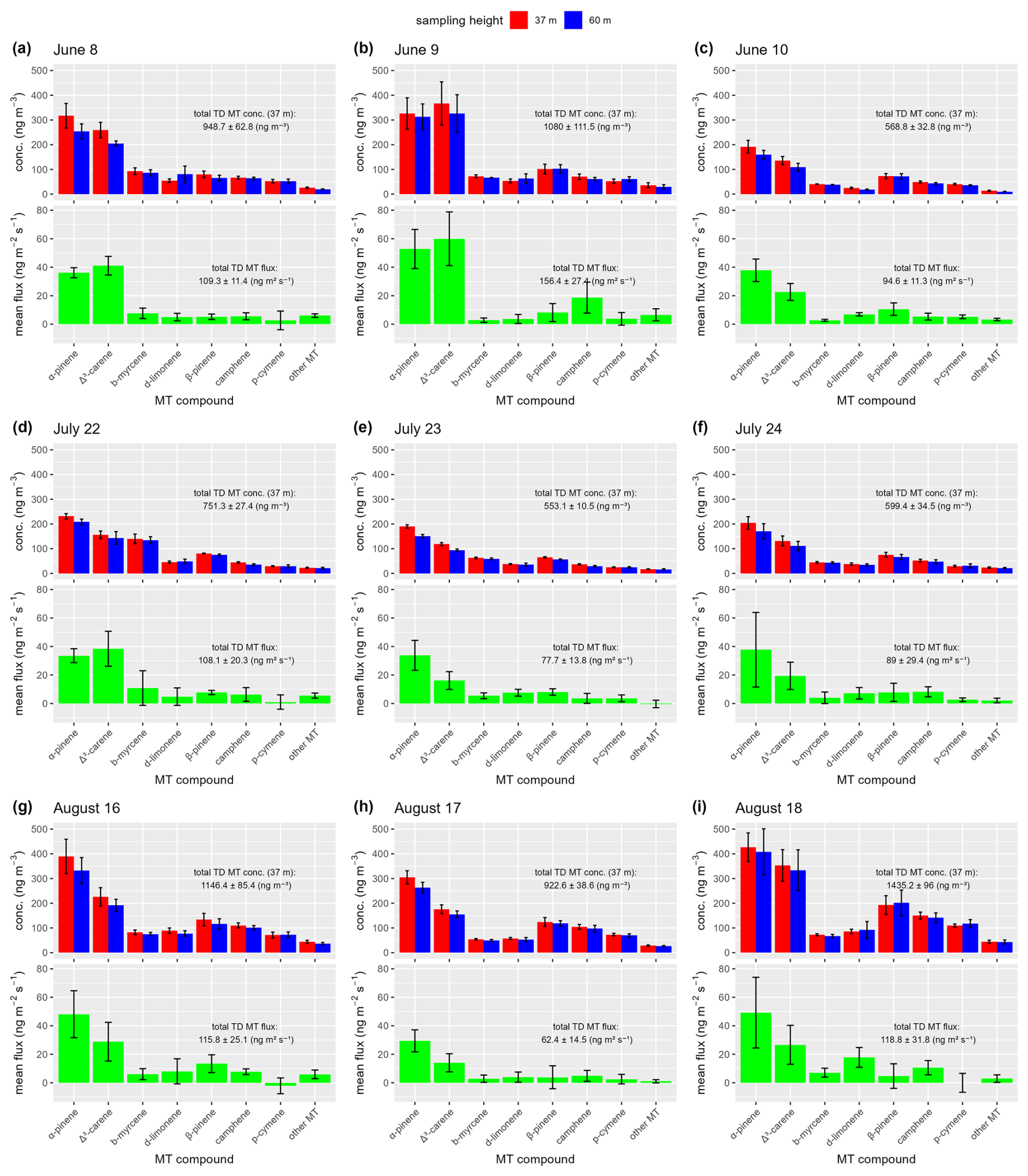
Figure C1 Daily mean (09:30–17:00 CEST) concentrations of MT compound species at 37 (red) and 60 m (blue) on the station flux tower at the ICOS Norunda boreal forest, as well as daily mean speciated MT fluxes (green), during 8–10 June (a–c), 22–24 July (d–f) and 16–18 August (g–i). Vertical error bars indicate the standard mean error.

Table C1 The ratios of momentum and sensible heat fluxes measured at 60 m to those at 37 m (i.e., $r_{u_{\ast }}=\stackrel{\mathrm{‾}}{u_{\ast ,\mathrm{60}\mathrm{m}}/u_{\ast ,\mathrm{37}\mathrm{m}}}$ and $r_H=\stackrel{\mathrm{‾}}{{\stackrel{\mathrm{‾}}{w{}^{\prime }T{}^{\prime }}}_{\mathrm{60}\mathrm{m}}/{\stackrel{\mathrm{‾}}{w{}^{\prime }T{}^{\prime }}}_{\mathrm{37}\mathrm{m}}}$) during daytime (08:30 am to 17:30 pm) during the 2020 Norunda campaign season. L is the Monin–Obukhov length.

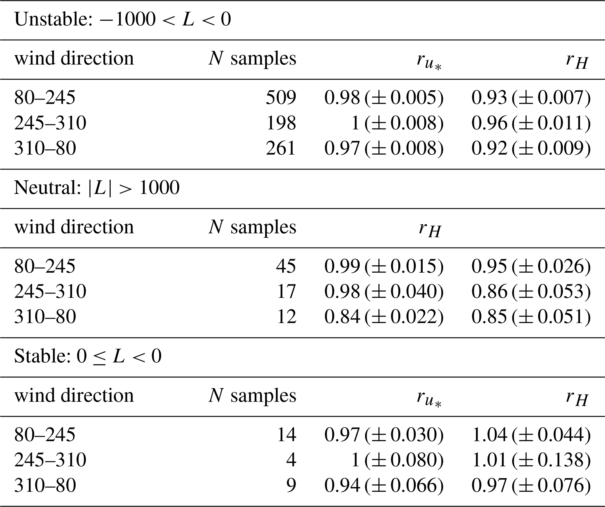
Table C2 Summary of VOC concentration calibration coefficients and parameters for the concentration (ppbv)-calibrated time series data for the 2020 Norunda field campaign measurements. For each calibrated compound, the summary includes the compound name, quantitative ion formula, observed mass-to-charge ratio $m/z$ [Th], molecular polarizability (α), permanent dipole moment (D), calculated proton-transfer reaction rate constant (kPTR), fraction f of the compound's total signal attributed to the quantitative ion, and average of the compound sensitivity (attenuated) during the full 2020 Norunda field campaign.

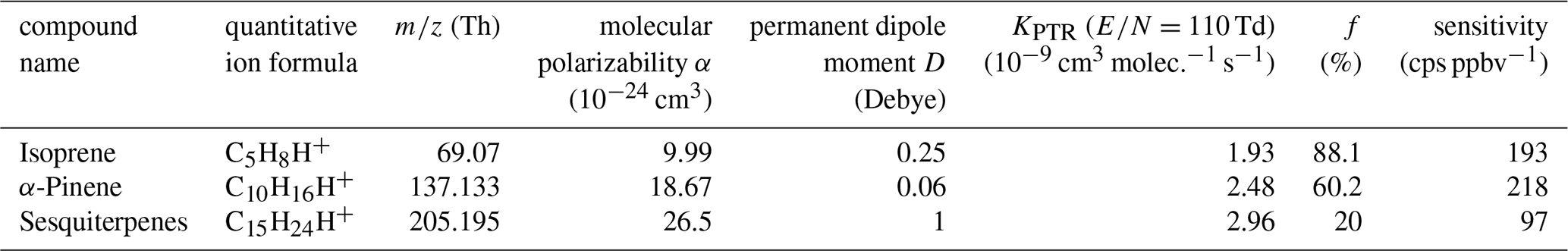
Table C3 Summary of reaction rate coefficients of terpenoids (isoprene, MTs, and SQTs) for OH, O₃, and NO₃ at 298 K and 1013.25 hPa air pressure at sea level. Reaction coefficients for isoprene and MTs are from Atkinson (1997) and reaction coefficients for SQTs are from Shu and Atkinson (1995). Typical values for their chemical lifetimes during the day (τ_c,day), night (τ_c,night), as well as the ratio of these day-night time scales (${\mathit{\tau }}_{\mathrm{c},\mathrm{day}}/{\mathit{\tau }}_{\mathrm{c},\mathrm{night}}$) are also included. Ambient day and night OH, O₃, and NO₃ concentrations for the calculation of τ_c,day and τ_c,night, are based on the modeled values used for the chemical degradation analysis. For comparison, typical values of the turbulent mixing time scale in the canopy during day and night (τ_t,day and τ_t,night, respectively) are ca. ${\mathit{\tau }}_{\mathrm{t},\mathrm{day}}=\mathrm{40}$ s, ${\mathit{\tau }}_{\mathrm{t},\mathrm{night}}=$ ca. 1.5 min, and ${\mathit{\tau }}_{\mathrm{t},\mathrm{day}}/{\mathit{\tau }}_{\mathrm{t},\mathrm{night}}=\mathrm{0.4}$–0.5.

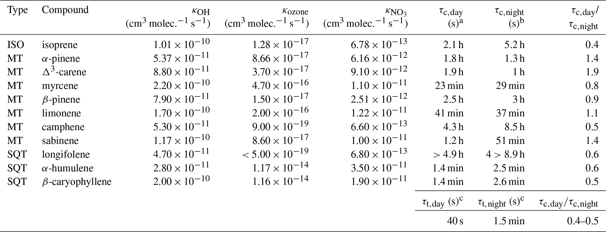
^a (daytime) OH and ozone concentrations are taken to be 1.2×10⁶ molec. cm⁻³ and 1×10¹² molec. cm⁻³ (ca. 0.05 ppt and 40 ppb), respectively. ^b (nighttime) OH and ozone concentrations are taken to be 3×10⁵ molec. cm⁻³ (ppt) and 5×10¹¹ molec. cm⁻³ (ca 0.01 ppt and 20 ppb), respectively. Nighttime NO₃: 2.5×10⁷ molec. cm⁻³ (ca. 2.5 ppt). ^c Based on ${\mathit{\tau }}_{\mathrm{t}}=z/u_{*}$ (e.g., Rinne et al., 2012) at inlet height (35 m) and typical friction velocities u_* observed during day and night (ca. 0.65 and 0.3 m s⁻¹, respectively) for the 2020 Norunda campaign.