Quantifying forest canopy shading and turbulence effects on boundary layer ozone over the United States

The presence of dense forest canopies significantly alters the near-field dynamical, physical, and chemical environment, with implications for atmospheric composition and air quality variables such as boundary layer ozone (O₃). Observations show profound vertical gradients in O₃ concentration beneath forest canopies; however, most chemical transport models (CTMs) used in the operational and research community, such as the Community Multiscale Air Quality (CMAQ) model, cannot account for such effects due to inadequate canopy representation and lack of sub-canopy processes. To address this knowledge gap, we implemented detailed forest canopy processes – including in-canopy photolysis attenuation and turbulence – into the CMAQv5.3.1 model, driven by the Global Forecast System and enhanced with high-resolution vegetation datasets. Simulations were conducted for August 2019 over the contiguous US. The canopy-aware model shows substantial improvement, with mean O₃ bias reduced from +0.70 ppb (Base) to −0.10 ppb (Canopy), and fractional bias from +9.71 % to +6.37 %. Monthly mean O₃ in the lowest model layer (∼ 0–40 m) decreased by up to 9 ppb in dense forests, especially in the East. Process analysis reveals a 75.2 % drop in first-layer O₃ chemical production, with daily surface production declining from 673 to 167 ppb d⁻¹, driven by suppressed photolysis and vertical mixing. This enhances NO_x titration and reduces O₃ formation under darker, stable conditions. The results highlight the critical role of canopy processes in atmospheric chemistry and demonstrate the importance of incorporating realistic vegetation-atmosphere interactions in CTMs to improve air quality forecasts and health-relevant exposure assessments.

1 Introduction

The Earth's vegetative canopies have ubiquitous effects on the physical, dynamical, and chemical environments, which impact the fluxes of momentum, heat, water, nutrients, and gases to the atmosphere above the canopy (Bonan et al., 2021, 2018, 2014). Some primary processes that alter the chemistry of the Earth's atmosphere due to the within canopy environment include radiative transport and photolysis (Monsi and Saeki, 1953; Nilson, 1971; Makar et al., 2017; Moon et al., 2020; Norman, 1979), turbulent transport and diffusion (Raupach, 1989; Harman and Finnigan, 2007, 2008; Ashworth et al., 2015; Makar et al., 2017; Bonan et al., 2018), hydrocarbon and other trace gas emissions (Guenther et al., 2012), and deposition to the leaves and foliage (Vermeuel et al., 2023). Understanding the importance of near-surface and canopy environments has led to decades-long measurements of heat, momentum, and trace gases and aerosols fluxes across different land surface types, vegetation properties, and forest/tree canopy characteristics (Baldocchi and Harley, 1995; Meyers et al., 1998; Hicks et al., 2016; Saylor et al., 2019; Hicks and Baldocchi, 2020). More recent field campaigns such as the Flux Closure Study 2021 (FluCS 2021) have studied the complex forest canopy chemistry and fluxes (e.g., reactive carbon fluxes) to attempt at closing budgets critical to atmospheric composition modeling across scales (Vermeuel et al., 2023).

Widely used chemical transport models (CTMs) in the community, such as the Community Multiscale Air Quality (CMAQ) model (Byun and Ching, 1999; Byun and Schere, 2006), have well represented processes that govern the Earth's atmospheric composition and air quality, including anthropogenic/natural source emissions, gas and aqueous chemistry, aerosol formation and physics, resolved horizontal/vertical transport, and dry/wet deposition (Appel et al., 2021); however, those CTMs often largely rely on the “big-leaf” approach that has minimal representation of sub-canopy structure and explicit processes (Bash et al., 2013; Pleim and Ran, 2011; Pleim et al., 2019, 2022). The big-leaf approach is readily used in land, weather, climate, and CTMs, and represents the plant canopies as a homogeneous single layer without real vertical structure (Bonan et al., 2021). This approach might be considered a reasonable simplification when atmospheric models routinely used horizontal resolutions (> 20 km) where a largely heterogeneous landscape within each grid cell could be represented only approximately anyway. Now, as horizontal resolutions of weather, climate and air quality models are becoming smaller, the adequacy of the big-leaf approach is being called into question. In addition, the big-leaf models and the chemical transport models in which they reside did not take into account the potential impact of changes in the vertical coordinate between the below-canopy and above-canopy environment (e.g. changes in light and temperature levels) on atmospheric chemistry, and of the vertical transport of pollutants from below- to above-canopy.

As an alternative to the big-leaf, single-layer canopy representations in CTMs, multilayer canopy models can resolve vertically varying profiles and microclimates in canopies (Baldocchi and Harley, 1995; Ogée et al., 2003; Chang et al., 2018; Bonan et al., 2021). The vertical distribution of leaf area has substantial impacts on the microclimate, leaf morphology, and leaf physiology in forest canopies, which in turn drives the dynamic/kinematic (e.g., wind speed and turbulent kinetic energy profiles), thermodynamic and radiative effects (e.g., daytime/nighttime air temperatures and light levels within and below the canopy) (see Bonan et al., 2021 and references found within). These in turn may drive chemical responses associated with the below-canopy environment to these changes (e.g., trace gas/scalar transport) characteristics of the sub-canopy layer. The use of a single-layer, “big-leaf” approach neglects such in-canopy profiles and their consequences, under the driving desire to adequately reproduce the behavior of multi-layer canopies to derive bulk quantities such as evapotranspiration from the canopy, and gross primary production. While the big-leaf simplification has over time proven useful in the sense that it is computationally efficient and can provide reasonably accurate fluxes, it can only be assumed to be “correct” under certain applications, namely large-scale influences of vegetation on large-scale climate (i.e., it is a “useful” approach). However, to best understand how large-scale climate effects manifest in the local, vertical, microclimate associated with vegetation requires the use of in-canopy parameterizations or more comprehensive multi-layer canopy (MLC) models. Furthermore, MLCs are explicitly needed to simulate chemistry and scalar transport in forest canopies (Boy et al., 2011; Wolfe and Thornton, 2011; Bryan et al., 2012; Saylor, 2013; Bonan et al., 2014; Ashworth et al., 2015). Overall, explicit in-canopy modeling can also better handle the natural complexity of trace gas and aerosol fluxes between the surface, vegetation, and atmosphere that are known to be important to Earth System, biogeochemical budgets (Braghiere et al., 2019).

MLC models have been incorporated in research versions of regional (e.g., Weather Research and Forecasting Model; Xu et al., 2017) and global (Community Land Model; Bonan et al., 2014, 2018) weather and climate models, and these previous studies have generally shown that the more detailed canopy representations can increase model accuracy in evapotranspiration. The understanding of the impact of the multilayer canopy on turbulence, and scalar transport has been long known (Raupach, 1989), and has been applied to one-dimensional canopy models that show good agreement with observations (Makar et al., 1999; Stroud et al., 2005; Saylor, 2013; Gordon et al., 2014; Ashworth et al., 2015). Only more recently have the effects of multilayer canopy models been scaled up to large eddy simulations with chemistry (Clifton et al., 2022; Fuentes et al., 2022) and to regional scale air quality forecast (AQF) models with more complex chemistry (Makar et al., 2017). Here, one of our main aims was to evaluate the effects of these processes on a regional scale CTM, CMAQ, in the community. A major limitation is that MLC models are more computationally costly and have proven problematic for widespread use and understanding in complex CTMs, necessitating the need for parameterized or simplified forms of these models that may reside within a more complex CTM, and capture the main features of the MLC models.

The CTMs used in the community and in operational forecasting centers continue to generate systematic ozone (O₃) overpredictions in the eastern US during the photochemical summer O₃ season (e.g., July–August). Such biases have been linked to distinct vertical gradients of O₃ measured within dense forest canopies of the US (Makar et al., 2017). Most CTMs and air quality forecasting models cannot capture such details, as they continue to rely on the previously discussed big-leaf model to represent canopy interactions with chemistry and scalar transport (Makar et al., 2017; Bonan et al., 2021). However, Makar et al. (2017) showed that inclusion of explicit sub-canopy effects of photolysis and the attenuation of light, in combination with the effects of sub-canopy vertical diffusivity in a regional-scale CTM, can improve predictions of near-surface O₃ concentrations in regions of contiguous canopies. It was further noted that simulated tropospheric O₃ in forest canopy regions is significantly reduced, through the combined effects of forest canopy shading (about $\mathrm{1}/\mathrm{3}$ of the total reduction) and modified turbulence (the remaining $\mathrm{2}/\mathrm{3}$), and that the inclusion of these in-canopy processes can largely correct this long-standing positive bias in forecasts of near-surface O₃ in the eastern US across multiple air-quality models (Makar et al., 2017).

The objectives of this work are to adapt the methodologies from Makar et al. (2017) and integrate them into relatively simple, but efficient parameterizations of in-canopy photolysis and turbulent diffusivity effects in the widely used CMAQ model. We then employ CMAQ process-analysis (PA) techniques, to better discern and quantify the in-canopy photolysis/chemistry and turbulence/transport effects on O₃ and other related chemical species and processes over the entire contiguous US region (CONUS). Apart from Makar et al. (2017), most studies on in-canopy chemistry and turbulence/diffusivity effects have been applied at local/field to near-local scales, while regional scale CTMs can better represent the widespread effects of in-canopy chemistry, turbulent diffusivity, and vertical transport across CONUS, and show how in-canopy processes interact with other processes in the atmosphere (such as advective transport and feedbacks between the canopy effects and meteorology). In this study, we focus on the primary effects of in-canopy photolysis attenuation and turbulence on chemical processes in CMAQ. While biogenic emissions and dry deposition are included in the model, they are represented using CMAQ's existing one-layer “big-leaf” method without explicit adjustments for vertical canopy structure. Section 2 describes the methods of the CMAQ model canopy parameterizations, CMAQ PA approaches, simulation design, observations, and evaluation protocol. Section 3 shows the results of the in-canopy parameterizations in CMAQ on O₃ and nitrogen oxides (NO_x), and a detailed evaluation and analysis of the impacts. Section 4 provides the study's main conclusions, a discussion on the limitations of the parameterizations, and paths forward to further improve integration of more comprehensive in-canopy processes for atmospheric composition models across scales.

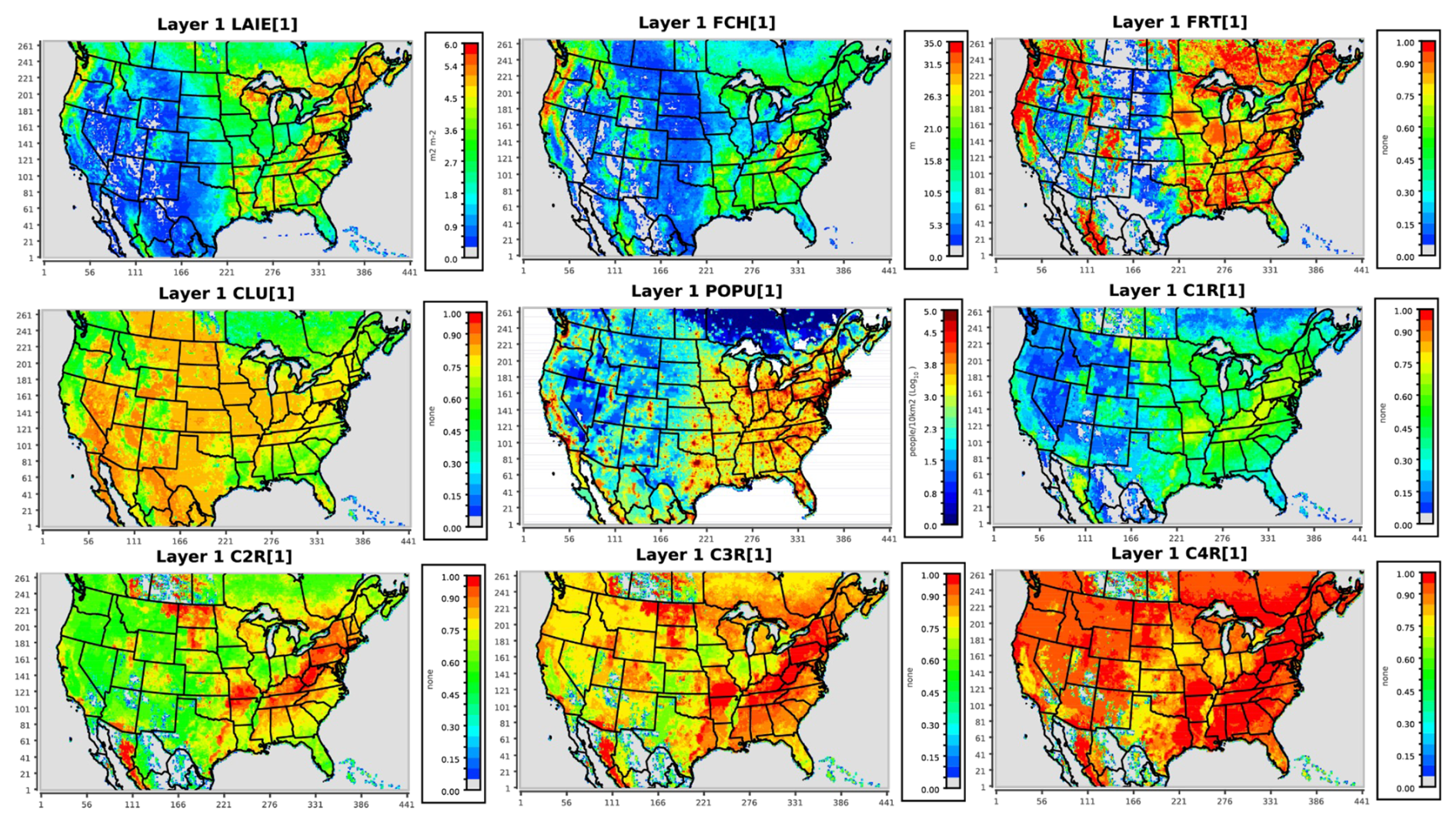
Figure 1 Spatial plots of average LAI, FCH, FRT, CLU, POPU, and CLAI_FRAC1-4 (referred to as C1R-C4R in headers) used for August 2019 CMAQ simulations in this work.

2 Methods

2.1 Gridded canopy datasets and contiguous canopy thresholds for CMAQ

A suite of gridded vegetative canopy-related parameters is needed for the new in-canopy parameterizations in CMAQ, as well as to define what model grid cells are representative of a contiguous canopy. These parameters include gridded 2-D fields such as the leaf area index (LAI), forest canopy height (FCH), forest fraction (FRT), and forest clumping index (CLU) based on Makar et al. (2017) (Fig. 1). The CLU is a unitless parameter ranging from 0 to 1 that describes the spatial distribution of foliage within the canopy. A CLU value of 1 indicates randomly distributed leaves, while lower values reflect increasing aggregation or “clumping” of leaf area (Makar et al., 2017; Chen and Black, 1992; Chen et al., 2005). The clumping index is used in conjunction with LAI to estimate the light extinction through the canopy and thus the fraction of direct radiation reaching the ground. These four canopy parameters are derived from a suite of ground-based datasets and space-borne observations including the MODerate Resolution Imaging Spectrometers (MODIS) on the NASA Terra and Aqua satellites. An additional dataset, population density (POPU), is used to identify and filter out city core areas that do not have contiguous vegetated canopies. To further approximate the vertical canopy structure spatially across the domain, we define four additional variables using the total LAI and cumulative LAI fractions (CLAI_FRAC) at four FCH-relative heights (0.75 × FCH, 0.50 × FCH, 0.35 × FCH, and 0.20 × FCH) within the canopy (Fig. 1). These heights were chosen to resolve the typical turbulence structure within forest canopies (Makar et al., 2017, Raupach, 1989). The CLAI_FRAC is based on typical leaf vertical distributions from the literature for different forest types (deciduous, coniferous, and mixed forests) assigned to the 230 Biogenic Emissions Landuse Database (BELD), version 3 (Pierce et al., 1998). These BELD data were weighted by the associated MODIS-based land use fractions in the model grid cell, and similar methods were used for CLU. More details on retrieval and processing of the gridded canopy variables may be found in Makar et al. (2017).

The first step in parameterization of the vegetative in-canopy effects is to determine whether a CMAQ model grid cell is defined as having a contiguous canopy with sufficient foliage to warrant defining a canopy column and correction. Based on similar theory from Makar et al. (2017), we apply the following canopy thresholds to define if a grid cell has a contiguous forest canopy:

1. The LAI exceeds a minimum threshold, suggesting that the grid cell likely has sufficient canopy shading or turbulence effects: LAI>0.1.

2. The canopy height (FCH) is substantial relative to the model's vertical resolution, such that it occupies at least one-fourth of the first model layer (which spans ∼ 40 m): FCH>10 m.

3. The population density is low enough to indicate that the grid cell is not dominated by urban influence: $\text{POPU}<\mathrm{10}\mathrm{000}\text{ people per }\mathrm{10}{\mathrm{km}}^{\mathrm{2}}(\text{i.e.},<\mathrm{1000}\text{ people per }{\mathrm{km}}^{\mathrm{2}})$.

4. The forest fraction (FRT) exceeds 0.5, indicating that more than half of the land use in the grid cell is covered by forest, consistent with a contiguous forest canopy: FRT>0.5.

5. The canopy is tall enough and dense enough to significantly reduce incident light reaching the surface, defined by the condition that less than 55 % of incoming light reaches the ground: $\text{EXP}(-\mathrm{0.5}\times \text{LAI}\times \text{CLU})<\mathrm{0.45}\text{ and }\text{FCH}>\mathrm{18}\mathrm{m}$.

We note that our FCH contiguous canopy condition #2 above (FCH > 10 m) updates that of Makar et al. (2017), which used a much lower FCH threshold (FCH > 0.5 m). We arrived at the FCH > 10 m threshold after numerous tests experimenting with 0.5, 3, and 10 m (along with all other canopy conditions applied), which resulted in a current best-case scenario regarding accurate regions of contiguous forests in the US simultaneously occurring with regions of CMAQ model systematic ozone overpredictions (see Fig. S1 in the Supplement). One implication of this finding is that vegetative canopies must be sufficiently “deep” for their effects to have an impact on regional scale atmospheric chemistry.

2.2 Vegetative in-canopy parameterizations in CMAQ

Here we describe the vegetative in-canopy parameterizations associated with the attenuation of light (photolysis) and the effects of modified turbulence (eddy diffusivity) based on Makar et al. (2017), as they have been implemented into the CMAQ model. We note that one significant difference in the implementation as described below is that the CTM vertical structure has been retained in its original form, unlike Makar et al. (2017) where additional vertical layers were added locally within canopy grid cells and model processes were split to operate on both the original CTM layer structure (in non-canopy grid cells) and an enhanced layer structure (in canopy grid cells), the latter including three additional layers. Here, the approach is to determine the impact of the canopy effects on the regional model layer structure, through calculation of CTM layer-thickness weighted photolysis attenuation and turbulent diffusivity reductions. While this approach does not explicitly resolve the canopy structure, it does provide estimates of its impact on the resolved vertical scale, requires less computational resources than the introduction of spatially varying local layers, and does not require the larger effort of recoding the CTM's core. The implementation of the full canopy layer structure within CMAQ for NOAA's Unified Forecast System is being implemented in ongoing work (Ivanova et al., 2024).

In-Canopy Photolysis: Using representative canopy conditions, the impact of attenuation of light due to a contiguous forest canopy can be parameterized in CMAQ for the jth model layer in the following way:

$$\begin{array}{}\text{(1)}& P\left(\mathit{\theta }z\right)={\displaystyle \frac{{\int }_{z_{j-\frac{\mathrm{1}}{\mathrm{2}}}}^{z_{j+\frac{\mathrm{1}}{\mathrm{2}}}}\text{exp}\left(-\frac{G\left(\mathit{\theta }\right)\text{CLU}\left(\mathit{\theta }\right)\text{LAI}\left(z\right)}{\text{cos}\left(\mathit{\theta }\right)}\right)\mathrm{d}z}{z_{j+\frac{\mathrm{1}}{\mathrm{2}}}-z_{j-\frac{\mathrm{1}}{\mathrm{2}}}}}\end{array}$$

whereP(θ,z) is the probability of beam penetration (i.e., fractional light penetration; Nilson, 1971; Monsi and Saeki, 1953), and depends on the LAI, leaf projection (G; for spherical assumption = 0.5), CLU, and solar zenith angle (θ). To capture the canopy vertical structure (i.e., leaf vertical distributions) in Eq. (1), we note that the LAI is dependent on height within the vegetation (LAI(z)), and that above the forest canopy height (z>FCH), the LAI is zero and the exponential term returns a value of unity (no light attenuation). To parameterize the integral effect of P(θ,z), we multiply the total LAI in the grid cell by the set of four CLAI_FRAC datasets (i.e.,g C1R-C4R) between the FCH and the four heights within the canopy (see Sect. 2.1 and Fig. 1), thus deriving the height-dependent photolysis attenuation factor. Linear interpolation between these attenuation values gives the attenuation profile below FCH. This vertically averaged probability of beam penetration is used as a correction factor on the j'th layer photolysis rates used in the CMAQ chemistry gas solver, which in turn affects the subsequent predictions of O₃, trace gas, and particulate matter concentrations.

In-Canopy Turbulence: In CMAQ, the near-surface scalar transport in the vertical is based on Monin–Obukhov (M-O) similarity theory (Monin and Obukhov, 1954) and calculation of the eddy diffusivity coefficient (K). Without presence of in-canopy effects, this calculation is based on the resolved meteorology taken in the native first model layer (closest to the surface); however, the fluxes and profiles in and above rough plant canopies deviate from M-O similarity theory due to the presence of a roughness sublayer (Bonan et al., 2018), where scalar transport is dominated by localized turbulence rather than large-scale advection (i.e., M-O theory cannot be used). Following the Makar et al. (2017) application of the Raupach (1989) near-field theory for many one-dimensional canopy models in the literature, and similar to our approach for photolysis, we adapt a methodology of vertically weighting the resolved layer values by a reduction factor referenced to an above-canopy height z₁, to parameterize in-canopy effects on turbulence/diffusivity in CMAQ, using the following two equations:

$$\begin{array}{}\text{(2)}& {\displaystyle }& {\displaystyle }{K}_{\text{can}}\left(z\right)={\displaystyle \frac{{\int }_{z_{j-\frac{\mathrm{1}}{\mathrm{2}}}}^{z_{j+\frac{\mathrm{1}}{\mathrm{2}}}}\frac{K_{\text{mod}}\left(z_{\mathrm{1}}\right)}{K_{\text{est}}\left(\frac{Z_{\mathrm{1}}}{\text{FCH}}\right)}{K}_{\text{est}}\left(\frac{z}{\text{FCH}}\right)\mathrm{d}z}{z_{j+\frac{\mathrm{1}}{\mathrm{2}}}-z_{j-\frac{\mathrm{1}}{\mathrm{2}}}}}\text{(3)}& {\displaystyle }& {\displaystyle }\left({\displaystyle \frac{z}{\text{FCH}}}\right)={\mathit{\sigma }}_{\mathrm{w}}^{\mathrm{2}}\left({\displaystyle \frac{z}{\text{FCH}}}\right)T_{\mathrm{L}}{\displaystyle \frac{z}{\text{FCH}}}\end{array}$$

where z is the height above the Earth's surface, z₁ is the height of the lowest model layer above the forest canopy, ${\mathit{\sigma }}_{\mathrm{w}}^{\mathrm{2}}$ the variance in Eulerian vertical velocity, T_L the Lagrangian turbulence timescale, and K_mod(z₁), ${\mathit{\sigma }}_{\mathrm{w}}^{\mathrm{2}}$ and T_L are dependent on the resolved friction velocity and atmospheric stability conditions from the driving meteorological model at the lowest model layer above the forest canopy (see Eqs. 4–9 in Makar et al., 2017), and that the effective in-canopy diffusivity, K_can(z), is normalized to allow a smooth transition between the K values for the resolved first model layer above the forest canopy and the reduced values within the forest canopy, $K_{\text{est}}(z_{\mathrm{1}}/\text{FCH})$. Effectively, the original CTM turbulent diffusivity coefficient profile K_mod(z) is weighted by a reduction factor which takes into account the typical shape of the observed diffusivity profile between the region above the canopy and the surface.

Here, this reduction has been vertically weighted to determine the net reduction in the CTM's vertical layer structure, in contrast to the approach in Makar et al. (2017) where additional vertical layers were explicitly added to the model vertical structure. The calculated values of K_can(z) are integrated downward through the sub-grid canopy in CMAQ at a vertical resolution of Δz = 0.5 m (same as for photolysis attenuation). This allows the parameterized sub-grid canopy effects to be incorporated into CMAQ without modifying its existing vertical layer structure. Specifically, the reduction in K is applied to the portion of the first model layer (∼ 0–40 m) corresponding to in-canopy heights (0–FCH), and to the portion above the canopy (FCH–40 m). This effectively introduces a separation in the above and below canopy environments, through reducing near-surface vertical transport in forest canopies. This can lead to higher concentrations of species emitted near the surface (e.g. nitric oxide, NO) that in turn influence other species (for example O₃, through enhanced O₃ titration in the same region that the photolysis rate reduction is reducing nitrogen dioxide, NO₂ photolysis). The reductions in vertical diffusivity also reduce the vertical transport/mixing of near-surface O₃ with the adjacent model layers above the canopy. In synergy with the in-canopy photolysis attenuation effects, the modified vertical diffusivity can thus, in part, further reduce predicted near-surface O₃ concentrations, and typical CTM overpredictions in regions of contiguous canopies.

We note that the in-canopy photolysis attenuation and turbulence/scalar transport parametrizations, as implemented here through vertical weighting of photolysis and turbulent diffusivity coefficient reductions for the CTM's vertical layers, add negligible computation time to the CMAQ routines, and are easier to implement in CTMs than the core model recoding required in the approach described in Makar et al. (2017). An additional important difference in the implementation here relative to Makar et al. (2017) is that the modifications to the coefficients of forest canopy turbulence are applied the driving meteorological model itself (rather than the scaled coefficients only being applied to the vertical transport of chemical tracers, as in Makar et al., 2017).

Dry deposition is retained as implemented in CMAQ v5.3.1 using the “M3Dry” scheme with one-layer “big-leaf” approach. While deposition rates respond to changes in near-surface concentrations and meteorological conditions, no vertical canopy structure is explicitly represented in the resistance terms. As such, the dry deposition parameterization is consistent with the default model configuration and remains unmodified in this study.

2.3 CMAQ process analysis

Process Analysis (PA) is a diagnostic tool (Jeffries and Tonnesen, 1994; Henderson et al., 2010) used to investigate and quantify complex processes leading to chemical concentration changes in the CMAQ model. The CMAQ model simulates the hourly air pollutant concentration, while PA provides the hourly process-based rates for selected air pollutants for each grid cell, including horizontal and vertical advection, diffusion, emission, dry/wet deposition, and chemical reaction rates (USEPA, 2022). Therefore, the PA diagnostics can be used to better quantify the effects of the forest canopy parameterizations and impacts on chemical concentrations in the CMAQ model. The PA results within chemical transport models (CTMs) include two key components: the integrated process rate (IPR), which accounts for hourly net chemical and physical processes, and the integrated reaction rate (IRR), which covers all chemical hourly reaction processing rates. The analysis tool, Python Environment for Reaction Mechanism/Mathematics (PERMM) (Henderson et al., 2009), is applied to study the IPR and IRR results. This study generated hourly IPR data for O₃, NO_x ($=\mathrm{NO}+{\mathrm{NO}}_{\mathrm{2}}$), volatile organic compounds (VOCs), and its composition for the simulated case studies (Sect. 2.3). The details of chemistry processing rates (initiation, propagation, and termination reactions) for all species in a reduced chemical mechanism (CB6r3) are used to quantify the O₃ and NO_x changes.

2.4 Simulation design, observations and evaluation protocol

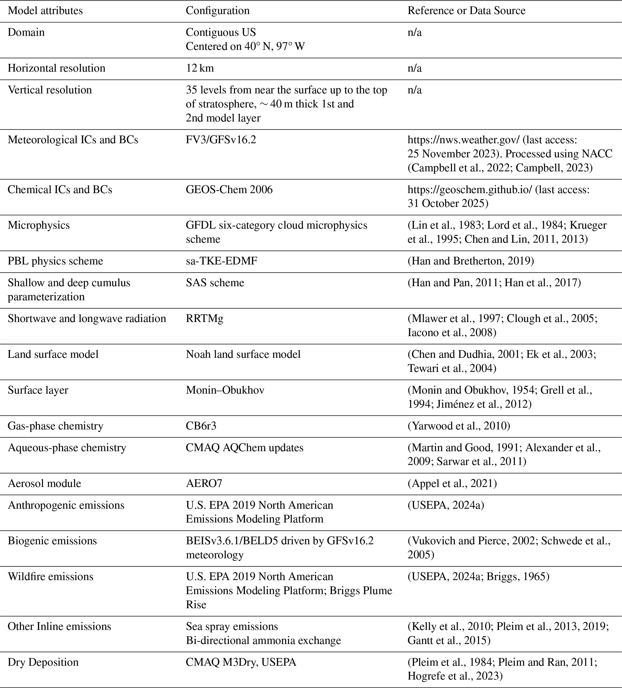
The model configuration used to implement and investigate the in-canopy parameterizations (Sect. 2.2) is based on a variant of the offline CMAQ model, version 5.3.1 (Appel et al., 2021). The updated CMAQv5.3.1 forest canopy shading, and turbulent diffusivity model codes (based on Eqs. 1–3) are available at https://zenodo.org/records/14502375 (last access: 3 November 2025) and https://github.com/GMU-CSER/CMAQ/releases/tag/GMU_Canopy_CMAQv5.3.1_05Aug2024 (last access: 3 November 2025). The meteorological driver is based on NOAA's operational Finite Volume Cubed Sphere (FV3) Global Forecast System (GFS) version 16.2, which was processed for model-ready CMAQ input by the NOAA-EPA Atmospheric-Chemistry Coupler (NACC), version 2.1.2, which is available at https://github.com/noaa-oar-arl/NACC/releases/tag/v2.1.2 (last access: 3 November 2025) (Campbell, 2023; Campbell et al., 2022). NACC is used to bi-linearly interpolate the canopy-related variables from Makar et al. (2017) including LAI, FCH, FRT, CLU, POPU, and C1R-C4R into the CMAQ grid used here (Fig. 1), which are needed for the updated forest canopy shading and turbulent diffusivity codes in CMAQ. These canopy variables are not available in the GFSv16.2 output files and thus are provided to NACC via external satellite and surface vegetation data sources (as discussed in Sect. 2.1), with conversion of these fields to the CMAQ grid being carried out through NACC. The overall meteorological and chemical model components, configurations, and other model inputs are shown in Table 1.

Table 1 The main meteorological (GFS) and chemical (CMAQ) model components and configurations used in this study. The abbreviation n/a stands for not applicable in this table.

To investigate and quantify the impacts of the in-canopy parameterizations using PA, we run two simulations: (1) “CMAQ-Base” without the canopy effects (hereafter referred to as the “Base” run), and (2) “CMAQ-Canopy” which includes the canopy effects as described above (hereafter referred to as the “Canopy” run). The canopy photolysis and diffusivity parameterizations are simultaneously turned on/off using a single CMAQ model environmental variable flag (i.e., “CTM_CANOPY_SHADE”, see updated scripts in code release: https://zenodo.org/records/14502375, last access: 3 November 2025). For the simulation period, we choose the month of 1–31 August 2019, with 10 d of spin-up (22–31 July 2019); the spin-up period is discarded and is not included in our analysis. The month of August was chosen because it is a representative warm summer month during both peak contiguous vegetative canopy conditions and high photochemical O₃ formation in the US. Thus, choice of this month allows for an ideal investigation of in-canopy photolysis attenuation and vertical turbulence/diffusivity effects on air quality. We select forest locations representing different US forest and ecosystem types for the case study to better understand their differences and canopy impacts on O₃ formation across CONUS (see Sect. 3 and Table 2 below), in addition to evaluating O₃ across the broader monitoring network.

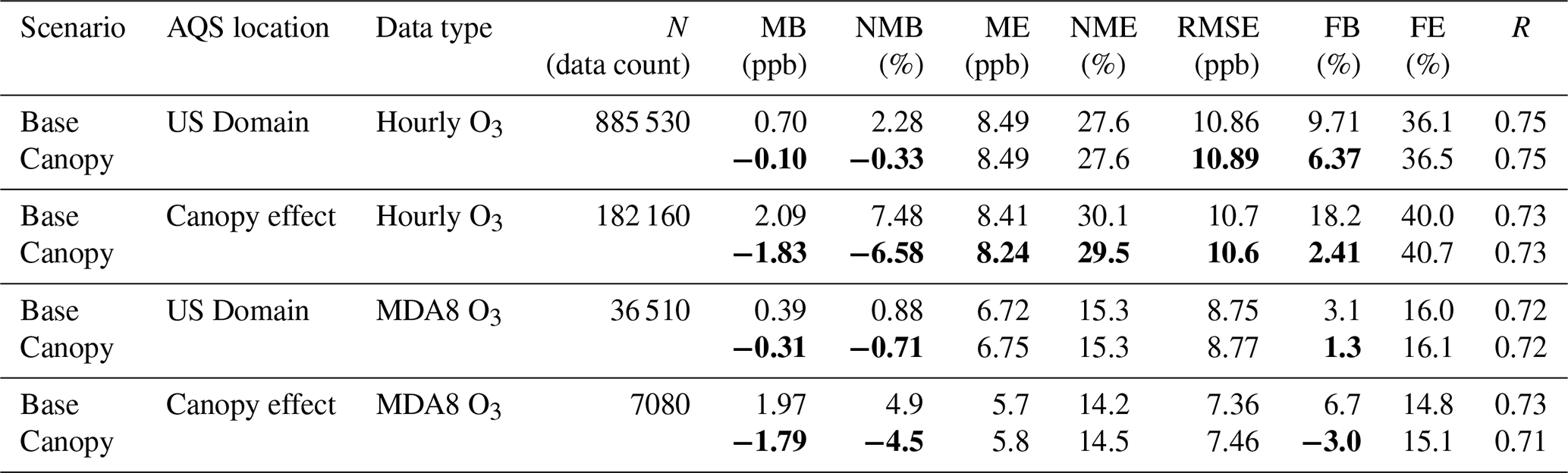
Table 2 Base and Canopy CMAQ model performance for hourly and MDA8 O₃ at all AQS sites and at AQS sites directly affected by canopy. The bold font indicates the improvement caused by the canopy effect.

The model evaluation includes comparison against observations from the U.S. EPA Air Quality System (AQS) O₃ (Parameter code: 44201) network (https://www.epa.gov/aqs, last access: 3 November 2025). For the O₃ observational data, 1217 sites across 48 contiguous US states are paired with modeling data, but only 235 of these sites fall within model grid cells that meet the criteria for a contiguous forest canopy as described above in Sect. 2.1 (see Sect. 3.1 and Fig. 2 below). We also note that the U.S. AQS observations sites are usually located in urban or suburban areas focused on relatively high population exposure and for public health impacts. Nevertheless, forest canopy processes affecting transported species such as ozone may influence concentrations of those species at locations downwind. As a result, about 19.3 % of O₃ sites have canopy effects in the simulations. Consequently, our study compares both the model performance changes for all US domain model-observational data pairs (i.e., both “direct” and “indirect” impacts) and canopy effect only model-observation pairs (i.e., “direct” impact). Direct effects are defined as grid cells that meet all five canopy criteria and activate the canopy parameterizations in CMAQ, while indirect effects are the grid cells that do not meet the criteria but may be influenced by canopy effect grid cells due to transport.

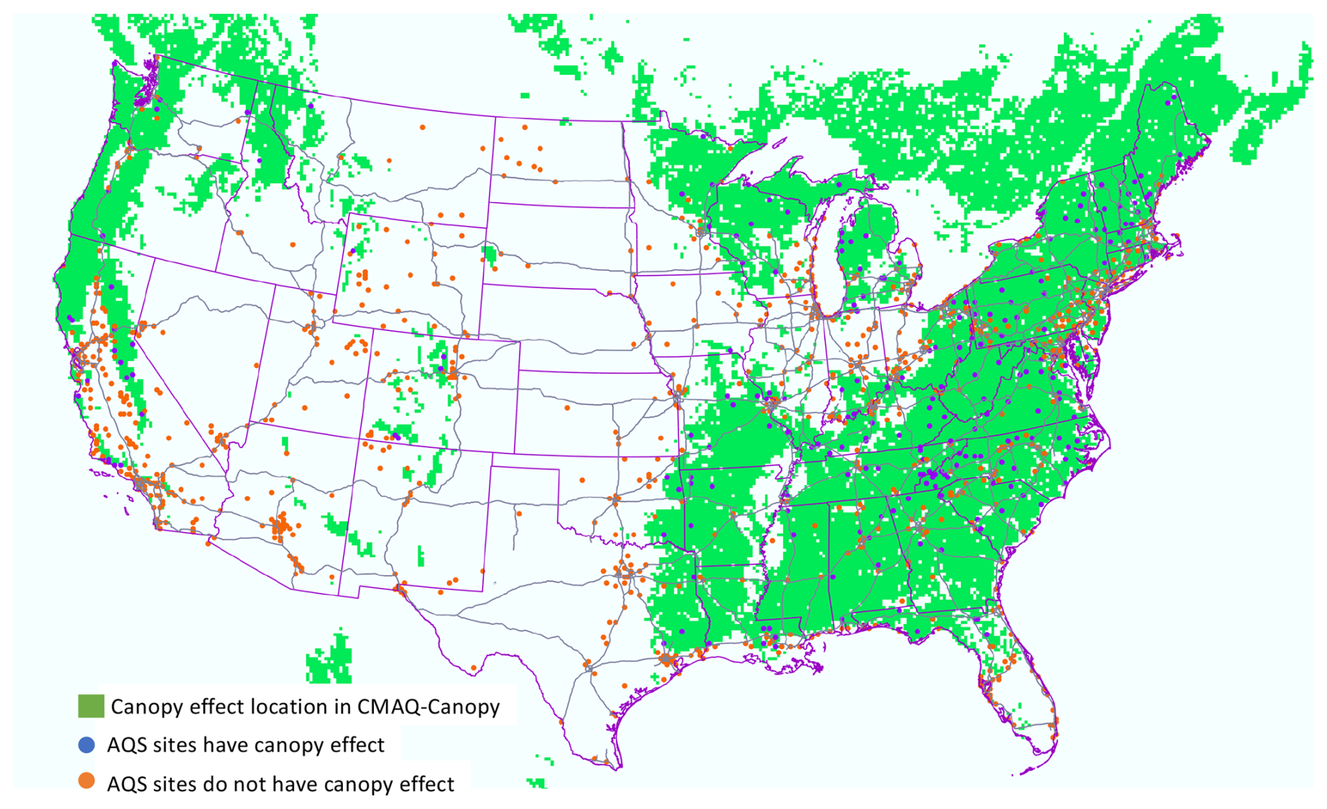
Figure 2 Model domain areas representing the canopy effect regions (green shading) for the Canopy scenario, overlaid with U.S. EPA AQS sites that are both directly (blue dots) and indirectly (orange dots) affected by the vegetative canopy parameterizations. The green shaded regions are derived from contiguous canopy thresholds described in Sect. 2.1 and generally shown in Fig. 1.

3 Results

3.1 Model performance

The Base and Canopy scenarios are evaluated to compare base model performance and demonstrate the impacts of canopy parameterizations (Sect. 2.2). Figure 2 illustrates the U.S. EPA AQS locations and the regions with vegetative canopy effects applied in the Canopy scenario. The green shaded regions are derived from contiguous canopy thresholds described in Sect. 2.1. The blue dots indicate AQS locations with direct canopy effects, while the orange dots correspond to grid cells which lack a forest canopy as defined here, and hence are subject to indirect effects. We note that many “indirect effect” grid cells (particularly in Eastern USA) appear within regions surrounded by forest canopies. Nevertheless, these grid cells do not meet the forest canopy selection criteria described above.

Table 2 presents the O₃ performance results (hourly average and Maximum Daily 8 h average, MDA8) for both model scenarios, including metrics such as data count (number of model-observation pairs used for the analysis) (N), mean bias (MB), mean error (ME), normalized mean bias (NMB), normalized mean error (NME), root-mean-squared error (RMSE), fractional bias (FB), fractional error (FE), and correlation coefficient (R). The mathematical definitions of those performance metrics are in the supplementary document. Across all model-observation pairs in the domain, the Base simulation demonstrates good overall performance for O₃ with a MB (NMB) of 0.70 ppb (2.3 %), a ME (NME) of 8.49 ppb (27.6 %), and an R of 0.75. This performance falls within documented photochemical model benchmark criteria (Emery et al., 2017).

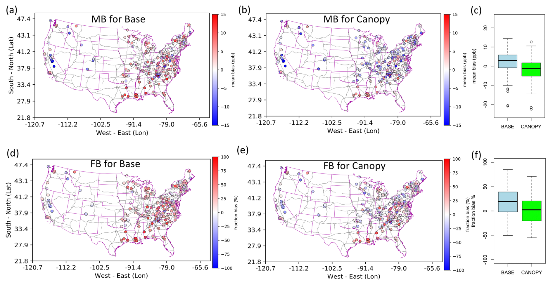
Figure 3 Hourly O₃ mean bias (MB) and fraction bias (FB) spatial plot at AQS sites with direct canopy effects. The upper panels (a–c) are MB for each site; the lower panels (d–f) are FB. The (a) and (d) are Base scenarios; (b) and (e) are Canopy scenarios. (c) and (f) are Box-whisker plots (blue = base; green = canopy) for MB and FB at canopy affected AQS sites, respectively. The boxes represent the interquartile range (IQR), with the upper and lower lines indicating the 75th (Q3) and 25th (Q1) percentiles, respectively. The thick line in the center of each box represents the median. The circle dots are outliers, defined as values lower than Q1–1.5 IQR or higher than Q3 + 1.5 IQR.

The Canopy scenario shows a clear improvement in MB (NMB) for O₃, from 0.7 to −0.1 ppb (2.3 % to −0.3 %), and in FB, from 9.7 % to 6.4 %, across all sites and hence including both direct and indirect canopy effects (Table 2). For sites that have canopy effect (blue dots in Fig. 2), the Canopy simulation improves most statistical performance measures (MB: 2.09 to −1.83 ppb; ME: 8.41 to 8.24 ppb; RMSE: 10.7 to 10.6; FB: 18.2 % to 2.41 %) for hourly O₃. While the MB represents the direct average difference between the observational data and the modeled data, the FB represents the difference between normalized observational and modeled data. Because the FB uses normalized differences for each paired prediction, it is less sensitive to the scale of the data (e.g., extremely high, or low values). Consequently, the MB shows an improvement but shifts from a relatively larger overestimation to a smaller underestimation in magnitude (US Domain: 0.7 to −0.1 ppb; Canopy effect location: 2.09 to −1.83 ppb). The FB still indicates that the model tends to overestimate O₃ (US Domain: 9.71 % to 6.37 %; Canopy effect locations: 18.2 % to 2.41 %), but the range of overestimation has largely decreased for hourly data in the Canopy run. The MDA8 O₃ for the entire domain has a MB change of 0.39 to −0.31 ppb (NMB is from 0.88 % to −0.71 %), while the Canopy effect locations have a MB change of 1.97 to −1.79 ppb (NMB is from 4.9 % to −4.5 ppb). However, the MDA8 O₃ FB differences are more substantial, with a change of 3.1 % to 1.63 % for the entire domain, and 6.7 % to −3 % for canopy effect locations. Thus, according to MB results, the Canopy effect improves the model MDA8 O₃ from slightly overestimated to slightly underestimated, and the FB result shows better improvement in reducing the overall model overestimation. The hourly O₃ concentration distribution, MB, and FB data for the canopy-affected AQS sites are presented in Fig. 3. Spatially, the hourly O₃ in the Base scenario is overestimated at nearly all canopy-affected sites in the eastern US (Fig. 3a).

Figure 3b shows significant improvement in reducing the O₃ overestimation at direct canopy effect sites with the Canopy scenario, particularly in Mississippi, Alabama, Florida, Arkansas, North Carolina, West Virginia, Virginia, Wisconsin, and Michigan. However, some AQS canopy sites show underestimation in the Base case, which worsens in the sites in Colorado and New York state. The MB values in Fig. 3a and b (N=235) are also represented by a box-whisker plot in Fig. 3c. In the Base case (blue box), around 75 % of the canopy AQS sites show overestimation, but the Canopy case demonstrates an improvement in reducing this overestimation. The FB results are shown in the lower panels of Fig. 3. The spatial plots in Fig. 3d and e depict the Base case and the improvement in the Canopy case, respectively, while Fig. 3f shows that the range and median FB values for the AQS sites are close to 0 % (no bias). Thus, the canopy-affected AQS sites show a clear improvement in reducing overestimation, as indicated by both MB and FB.

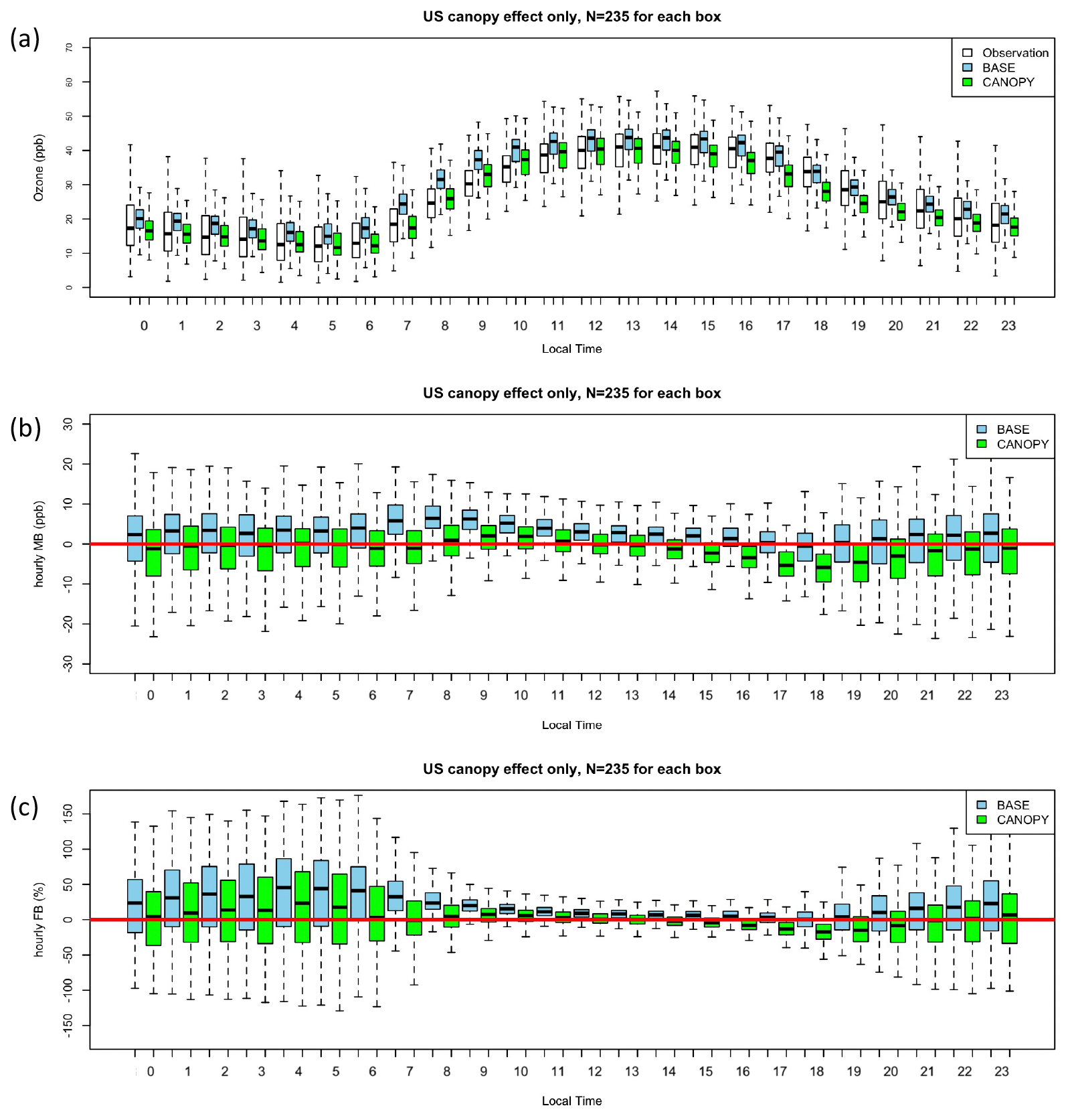
Figure 4 (a) Near-surface (first model layer) diurnal hourly average O₃ concentration (ppb) for canopy-affected AQS sites. Each box represents the monthly hourly average of all AQS sites (235 sites). The white box represents the AQS observations, the blue box is for the BASE case, and the green box is for the Canopy case. (b) Mean bias (MB, in ppb) for the paired data, and (c) Fractional bias (FB, in %) for the same paired data between the AQS observations and the model results. The blue box represents the BASE case, and the green box represents the Canopy case. The bias plots (b and c) show the hourly performance of the model in comparison to the AQS observations. The hourly MB and FB median values are present is Table S3.

Figure 4 shows that the canopy parameterization improves the diurnal pattern of hourly mean O₃ concentrations at most AQS sites affected by canopy effects. Between 09:00 and 14:00 LT (local time), the Canopy simulation better captures the observed spread in ozone levels, with its vertical extent more closely aligning with the broader distribution seen in observations than the Base case. This suggests that the updated parameterization more accurately represents the magnitude of daytime ozone variability. The enhanced spread in the Canopy case arises from the more discrete and intermittent nature of turbulent eddies, as represented by Raupach's near-field approach to vertical diffusivity (Eqs. 2 and 3). This formulation suppresses vertical diffusivity near the canopy top, particularly under stable or weakly mixed conditions, which can lead to localized accumulation or depletion of ozone within the canopy layer, thereby increasing spatial and temporal variability across sites and hours.

Diurnally, the BASE model scenarios overestimate O₃ from 12 AM to 5 PM and 9 PM to 11 PM local time (LT), while the Canopy case shows O₃ mean ranges closer to observations (Fig. 4a). For a relatively narrow period of 5 PM to 7 PM LT, however, the Base case performs better, whereas the Canopy case shows a larger underestimation for most AQS sites. Figure 4b represents the MB calculated from paired data, and Fig. 4c shows the FB. Figure 4b and c illustrate that daytime (8 AM to 4 PM LT) O₃ concentrations are higher (AQS mean Inter-Quartile Range (IQR) is 32 to 42 ppb at 12 PM LT; Base is 38 to 43 ppb; Canopy is 35 to 40 ppb) but exhibit lower bias (Base: IQR of MB is 0.9 to 5 ppb at 12 PM LT; FB is 3.7 % to 14 %). The Canopy case improves the overestimated O₃ ranges and comes closer to centering the range around the perfect score values (Canopy: IQR of MB is −2.4 to 2.4 ppb at 12 PM LT; FB is −4.8 % to 8.3 %). Nighttime O₃ concentrations (6 PM to 6 AM LT) are lower (AQS hourly mean IQR is 12.3 to 24 ppb; Base is 17 to 23 ppb; Canopy is 13 to 19 ppb) but have larger bias ranges (BASE: IQR of MB is −4.3 to 7.0 ppb at 12 AM LT; FB is −18 % to 57 %). The Canopy effect reduces the overestimation seen in the Base case (Canopy: IQR of MB is −8 to 3.6 ppb at 12 AM LT; FB is −36 % to 40 %), again centering the biases about the zero better than the base case.

The largest improvement due to the canopy effect happens in the morning at 8 AM. The AQS hourly mean IQR is from 20 to 29 ppb at 8 AM LT, the Base case IQR is 29 to 34 ppb, while the Canopy case is much closer at 23 to 29 ppb. The paired data also shows the improvement from Base case (IQR range of MB is from 3.9 to 9.5 ppb at 8 AM LT; FB is from 15 % to 38 %) to Canopy case (IQR of MB is from −3.0 to 4.7 ppb at 8 AM LT; FB is from −10 % to 20 %). These results illustrate the canopy effect on improving CMAQ's overall diurnal O₃ patterns during both daytime and nighttime, with some degradation with larger underestimations in late afternoon and early evening (e.g., 5 to 7 PM LT).

3.2 Canopy impacts on O₃

In regions with direct canopy effects, the canopy parameterizations in CMAQ lead to forest shading and reduced photolysis during the daytime, and reduced transport of O₃ and other titrating molecules during the nighttime (in agreement with Makar et al., 2017). These processes collectively reduce the mean level of the near-surface (i.e., first model layer) O₃ diurnal profile in the Canopy simulation compared to the Base case (Fig. 4). Overall, the Canopy simulation demonstrates an improved O₃ diurnal profile and reduces overestimation (especially FB) compared to AQS observations. However, direct canopy effects can also exacerbate Base CMAQ underpredictions during some hours of the later afternoon and evening. To provide more insight on this result, the following sections comprehensively analyze, discuss, and quantify the impacts of the canopy parameterizations in the lowest model layers for O₃ and related NO_x processes using CMAQ-PA.

3.2.1 Effects of the canopy on O₃ concentrations in the US

For August 2019, higher monthly average O₃ concentrations in the first (approximately 0–40 $\mathrm{m}\mathrm{a}.\mathrm{g}.\mathrm{l}.$) and second model layers (approximately 40–90 $\mathrm{m}\mathrm{a}.\mathrm{g}.\mathrm{l}.$) are observed in mountainous and suburban areas near Los Angeles, Denver, Salt Lake City, Chicago, Detroit, and New York City (Figs. 5a and 6a). The widespread effects of the canopy parameterizations result in significant reductions in the first model layer monthly average O₃ concentrations for Canopy compared to Base, particularly in the dense forest regions of the eastern US, with a maximum grid cell decrease of about 9 ppb (Fig. 5b). However, the canopy effects also lead to increases in the second layer O₃ concentration, with a maximum increase of about 3 ppb (Fig. 6b). Hence, we next use CMAQ-PA to further diagnose and quantify the contrasting canopy impacts on first and second model layer O₃ concentrations.

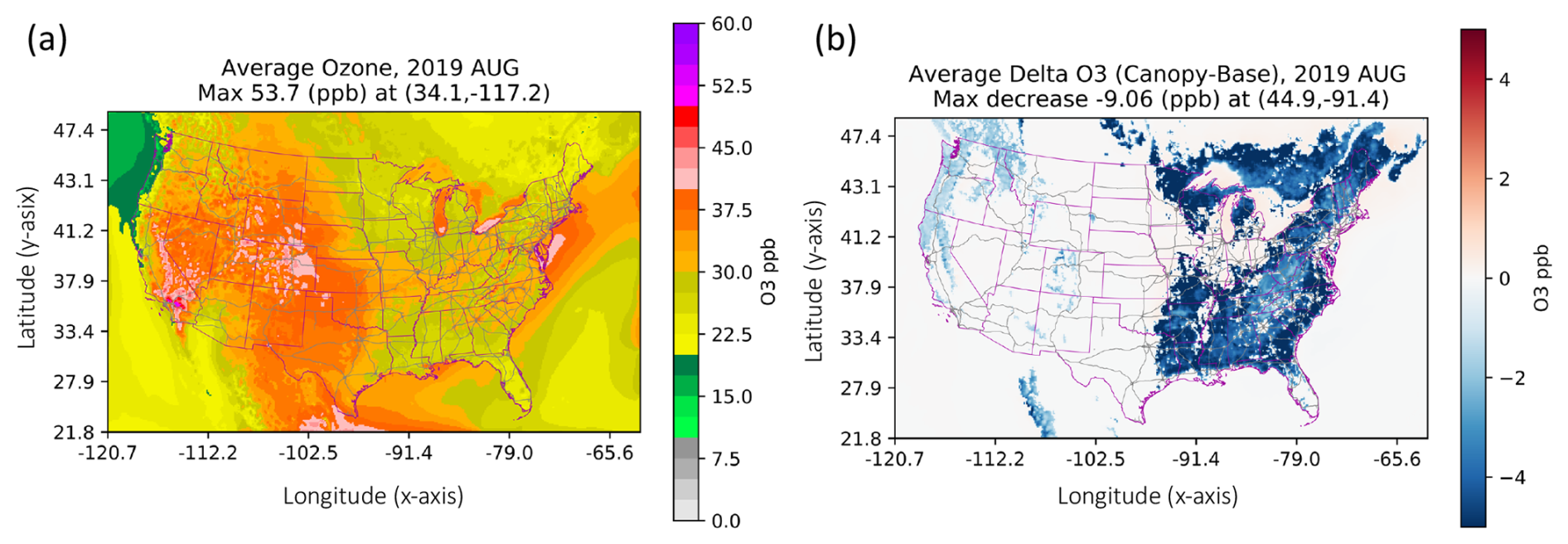
Figure 5 First layer(0–40 m) Base case monthly average O₃ concentration (a) and the monthly average difference (b) between Canopy case and Base case (Canopy – Base) in 2019 August.

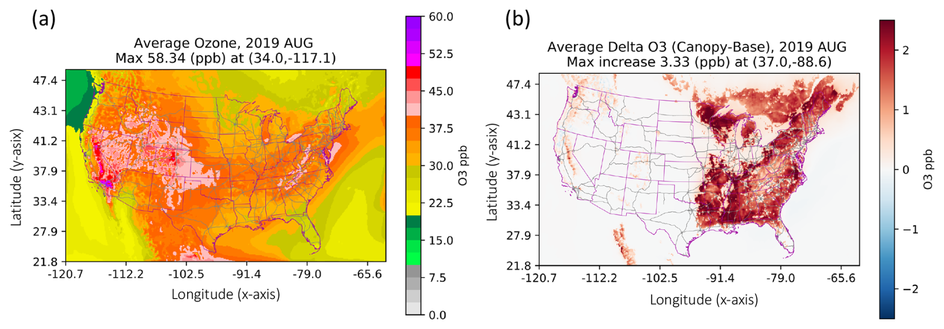
Figure 6 Second layer (40–90 m) Base case monthly O₃ concentration (a) and the difference (b) between Canopy case and Base case (Canopy – Base) in 2019 August.

3.2.2 PA results for canopy-effected modeled first layer (0–40 m) O₃ changes

The direct canopy effect locations, shown as green shaded areas in Fig. 2, are selected for studying O₃ changes using CMAQ PA output. We also applied a time zone mask for selecting the eastern standard time (EST) region to provide emphasis of the eastern US and thus inherently reducing impacts from the western mountainous regions. To investigate the diurnal patterns for processing rates, the PA data are calculated as 1 month averages for each hour and canopy-effected grid cells. The major processes that contribute to O₃ changes are vertical diffusion rate (“v diffusion”, green lines), deposition rate (orange lines), and chemical processing rate (red lines) in the morning (Fig. 7a).

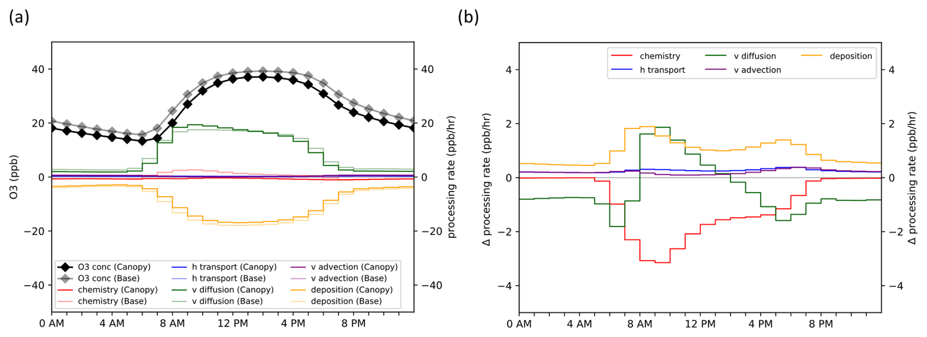
Figure 7 Hourly average near-surface O₃ (0–40 m above surface) process analysis result at Canopy effect locations in August 2019 for (a) two scenarios (Canopy: solid shade, Base: transparent shade) and their process rate differences (Canopy – Base) in (b).

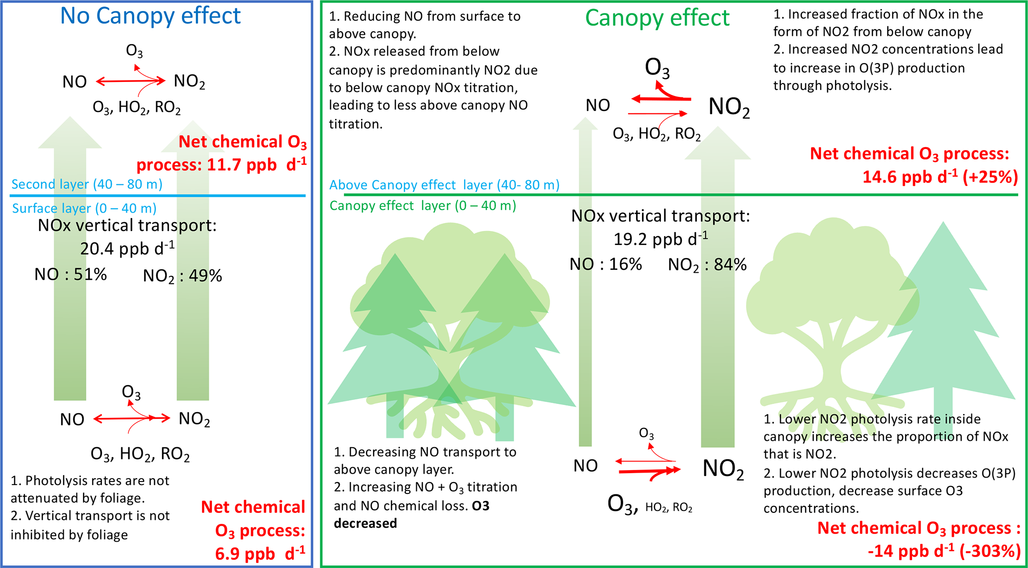
The Base case (transparent shaded lines in Fig. 7a) shows that vertical diffusion processing rates (transparent green line) contribute significantly to near-surface O₃ concentrations, with a maximum of 18 ppb h⁻¹ at 9–10 AM. Deposition causes the major loss, with a maximum of 18 ppb h⁻¹ at 12–1 PM. The chemical production rate of O₃ (transparent red line) reaches a maximum of 3 ppb h⁻¹ at 9–10 AM during the daytime but becomes negative during the nighttime (7 PM–5 AM). These results indicate that surface O₃ changes in the Base case originate from exchange of O₃ with the upper troposphere, near-surface O₃ chemical production and loss, and loss via deposition to the surface.

In the Canopy case (solid shaded lines in Fig. 7a), the daytime maximum near-surface O₃ chemical production rate within the first model layer (red line) becomes all negative (maximum: −1 ppb h⁻¹) compared to the Base case. This suggests net chemical loss of O₃ within the canopy, where the chemical processing rate difference reaches a maximum of −3 ppb h⁻¹ at 9 AM (Fig. 7b). The reduction in chemical processing rate is caused by decreased NO₂ photolysis resulting in less O(³P) formation and hence less O₃ formation, while at the same locations, the relative amount of NO_x that remains as NO increases due to trapping of fresh emissions, and hence the O₃ titration rate increases, leading to increased O₃ destruction. The net result is a shift from net chemical production to net loss of near-surface O₃, in areas of contiguous canopies.

Additionally, there is a reduction in vertical transport rates due to the impact of contiguous canopies on modulating the eddy diffusivity rates in the lowest model layer (Fig. 7b). It is important to note that the quantities depicted in Fig. 7b are the differences in the rates of change between the two simulations; a negative value indicates that the rate of change has decreased with the canopy parameterization, a positive value indicating that the rate of change has increased. A negative value for the vertical diffusion component (Fig. 7b, green line) thus indicates that the rate of change associated with vertical diffusion has decreased, but not necessarily that the rate of change associated with transport is negative, in either simulation.

The vertical diffusion processing rate (Fig. 7b, green line) differences for CMAQ (Canopy-Base) in the first model layer are negative starting in the afternoon (2 PM) and through nighttime into the early morning (5–8 AM LT) by up to −1.8 ppb h⁻¹. This is due to canopy impacts on relatively less diffusion of higher O₃ concentrations downward in conjunction with chemical net loss of O₃ (from shading and reduced photolysis in mid-afternoon and early morning) in the first model layer (red line). Consequently, the Canopy case develops a larger vertical O₃ concentration gradient between the first and second model layers from 7 PM – 7 AM (see Figs. 8 and S1 for O₃ vertical profile and PBL height).

We note that the rate of change of O₃ due to vertical diffusion $\partial \left[{\mathrm{O}}_{{\mathrm{3}}_{\mathrm{vdiff}}}\right]/\partial t$ can be expressed as:

$$\begin{array}{}\text{(4)}& {\displaystyle \frac{\partial \left[{\mathrm{O}}_{{\mathrm{3}}_{\mathrm{vdiff}}}\right]}{\partial t}}=-\left\{{\displaystyle \frac{\partial K}{\partial z}}{\displaystyle \frac{\partial \left[{\mathrm{O}}_{\mathrm{3}}\right]}{\partial z}}+K{\displaystyle \frac{{\partial }^{\mathrm{2}}\left[{\mathrm{O}}_{\mathrm{3}}\right]}{\partial z^{\mathrm{2}}}}\right\}.\end{array}$$

From Fig. 8 (and Fig. S2), it can be seen that ${\partial }^{\mathrm{2}}\left[{\mathrm{O}}_{\mathrm{3}}\right]/\partial z^{\mathrm{2}}$ is always greater at the second model layer with the use of the canopy parameterization, though weaker above layer 2, and in the early morning, $\partial \left[{\mathrm{O}}_{\mathrm{3}}\right]\partial z$ is less with the canopy model above layer 2, and greater below layer 2, and by the late morning the vertical gradients above the lowest model layer are relatively unchanged. That is, the effects are strongest and extend into the first three layers when the magnitude of K is relatively low (nighttime and early morning). By late morning, with the diurnal increase of K, the canopy affects only be seen in the lowest model layer.

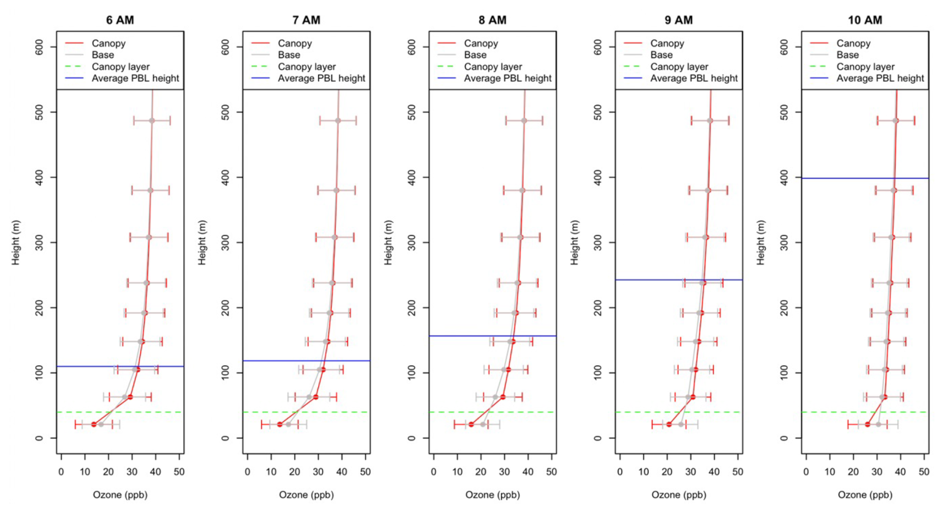
Figure 8 The hourly vertical O₃ profiles of Base (gray) and Canopy (red) at 6 AM to 10 AM LT. The dots in each layer are average O₃ concentration in regions of canopy effects in Fig. 2 and the range bars are the standard deviation range. The blue Line is the hourly average PBL height, and the green dash line is the forest canopy height.

At 8 AM, the average planetary boundary layer (PBL) height increases to 160 $\mathrm{m}\mathrm{a}.\mathrm{g}.\mathrm{l}.$ (higher than the fourth layer), in response to morning increases in the magnitude of K, which allows for more O₃ that had previously built up in the free troposphere transport downward into the PBL (Fig. 8). This results in increases to the vertical diffusion O₃ processing rate of about 1.5–2 ppb h⁻¹ for the canopy compared to Base case between 8 AM–2 PM in the first model layer (Fig. 7b). In other words, the presence of the canopy via the modified K profile delays the downward transport of higher O₃ aloft (due to buildup during late afternoon, evening, and early morning) until the PBLH grows high enough into the region where the canopy increased gradient dissipates after 8 AM LT. Therefore, the first model layer O₃ changes due to the canopy (i.e., net decrease all hours; see black lines in Fig. 7a) is caused by both decreased photolysis and modulated vertical diffusion processes. The reduction of near-surface O₃ concentration also reduces the deposition rate (Fig. 7a from −14 to −12 ppb h⁻¹ at 8 AM LT).

3.2.3 PA results for canopy-effected modeled second layer (40–90 $\mathrm{m}\mathrm{a}.\mathrm{g}.\mathrm{l}.$) O₃ changes

Unlike the first (lowest) model layer (0–40 $\mathrm{m}\mathrm{a}.\mathrm{g}.\mathrm{l}.$) that always has positive O₃ vertical transport process (upper layer O₃ are transported to surface by diffusion), the second layer vertical transport processes in the Base run (Fig. 9a, diffusion, green transparent line) only shows positive in the morning hours of 8 AM to 11 AM LT. Figure 9a is presented in duo y-axis, the left y-axis is concentration, and the right y-axis is processing rate.

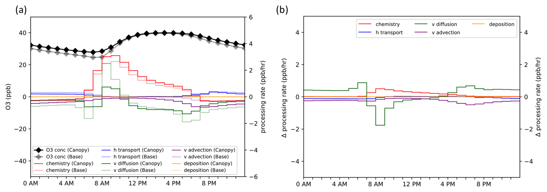
Figure 9 Hourly average 2nd layer (40–80 m above surface) O₃ process analysis result at Canopy effect locations in August 2019 for (a) two scenarios (CMAQ-Canopy: solid color, CMAQ-Base: transparent color) and their differences (Canopy – Base) in (b).

From midnight to early morning (0 AM to 6 AM LT), the loss of second layer O₃ transported downward (v diffusion) to the first model layer is reduced due to the canopy (transparent green line to solid green line). At 6 AM LT (sunrise), the PBL height is above the second model layer height at roughly 110 m (close to the third model layer height; Fig. 8), and the chemical O₃ formation process has become positive (Fig. 9a; Base: 0.47 ppb h⁻¹, Canopy: 0.5 ppb h⁻¹). At 7–8 AM LT, the increase of O₃ concentration gradient (∼ 15 ppb between first and second model layer) further demonstrates the one-hour delay in vertical diffusion from the second layer down to the first model layer (see Fig. 9a, green line at 6–8 AM). This emphasizes the effect of the canopy in building up O₃ concentrations in the second model layer over the late afternoon, evening, and early morning hours (Fig. 9b; positive net O₃ difference, green line) that also sharpens the concentration gradient between the first and second model layers during these hours.

During the morning hours (8 AM to 11 AM LT), the PBL height is above the fourth model layer and there is a smaller concentration gradient between the third layer and the second layer in the Canopy case compared to Base (Fig. 8). Hence, there is relatively less O₃ transport from the third layer into the second model layer due to the canopy (Fig. 9a, green lines; 8 AM to 11 AM LT). In the afternoon hours of 12 PM to 4 PM LT, the PBL height grows higher, and O₃ concentration reaches an equilibrium state between the third and second layers (Fig. S2), resulting in minimum diffusion transport from the third to the second layer. Although there is almost no O₃ transport from the third to the second layer, the additional chemical formation of O₃ in the second layer (due to canopy-imparted NO_x changes; see Sect. 3.2.4) increases O₃ concentrations and resulting transport to the first model layer, as reflected in the increased vertical transport (diffusion and advection) loss processing rate (green and purple line; Fig. 9b at 12 PM to 4 PM LT). At nighttime between 8 PM to 5 AM LT, there is no new O₃ formation (rather destruction) in the second layer, while the canopy effect reduces O₃ diffusion loss from the second layer to the surface layer (green and transparent green lines; Fig. 9a) but increase the O₃ advection loss from second layer the surface layer (purple and transparent purple lines; Fig. 9a). Considering summation of all vertical processes, the diffusion process is still larger than the advection process. This further reemphasizes that as a result, the O₃ concentration in the second layer is higher at night in the Canopy run.

The chemical processing rate contributes substantially to O₃ concentration during photochemical daytime hours (6 AM to 6 PM) in the second model layer (transparent and solid red lines in Fig. 9a). In the Canopy case (solid red line), the O₃ chemical processing rate increases during all daytime hours compared to the Base case, maximizing at about 0.5 ppb h⁻¹ at about 8–9 AM. To investigate the reasons leading to the chemically induced O₃ increase in the second layer for the Canopy case, we investigate the NO_x PA in the first model layer, which is the closest model layer to major NO_x emission sources at the surface.

3.2.4 PA results for canopy-effected modeled NO_x

Figure 10 shows the first layer NO_x concentration and total processing rates (10a for NO_x, 10d for NO, and 10g for NO₂), explicit processing rates results (10b for NO_x, 10e for NO, and 10 h for NO₂), and delta processing rates (Canopy- Base) (10c for NO_x, 10f for NO, and 10i for NO). In Fig. 10 first row, the canopy leads to increases in NO_x concentrations in the first model layer (Fig. 10a; month average difference: +0.16 ppb, +13.6 %), and the PA results show that the increase is caused by the reduction of vertical transport loss from the first to second model layer (Fig. 10b; transparent and solid green lines, maximum difference at 6 AM, −0.02 ppb h⁻¹) and reduction of chemical loss at 7 AM to 7 PM. (Fig. 10b; transparent and solid red lines, maximum difference at 8 AM, −0.05 ppb h⁻¹). Section 3.3 explains the details of the NO_x chemical reaction changes. For other processing rate of NO_x, the horizontal transport (blue line) and vertical advection (purple line) of NO_x are nearly identical between the two simulations, and hence the change in horizontal transport and vertical advection are minimal (Fig. 10c).

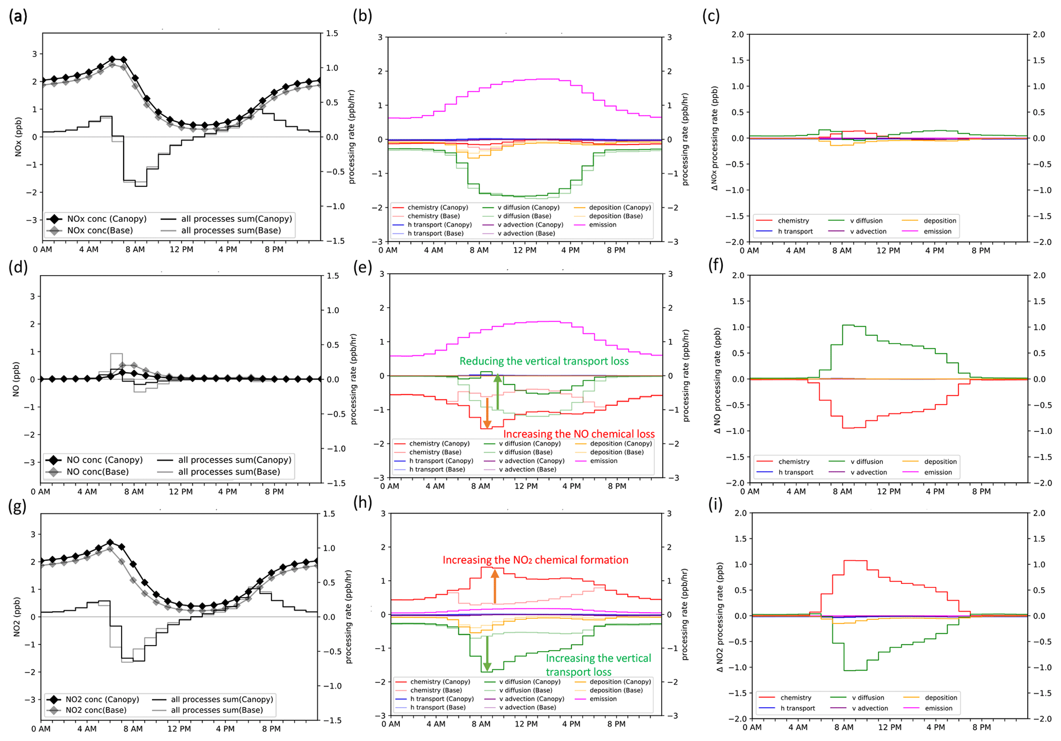
Figure 10 Hourly average surface layer (0–40 $\mathrm{m}\mathrm{a}.\mathrm{g}.\mathrm{l}.$) process analysis result for (a) NO_x concentration and net process; (b) NO_x explicit processing rates; (c) delta (Canopy- Base) NO_x processing rate (d) is NO concentration and net process; (e) is NO explicit processing rates; (f) delta (Canopy- Base) NO processing rate (g) is NO₂ concentration and net process; (h) is NO₂ explicit processing rate and (i) delta (Canopy- Base) NO₂ processing rates at Canopy effect locations in August 2019 for two scenarios (Canopy and Base).

Figure 10 s row presents the NO PA results. Most NOysources in the first model layer are due to surface emissions, with a monthly average rate of 0.95 ppb h⁻¹ (Fig. 10e, magenta line). The Canopy case reduces the vertical diffusion loss (i.e., more trapping) of NO from the first to second model layer, with a maximum difference at 9 AM of +1.1 ppb h⁻¹ (Fig. 10f; solid green lines). This inherently leads to an increase in the NO chemical loss rate of via various chemical processing pathways (e.g., NO + O₃, HO₂, or RO₂ → NO₂, see shift from Base transparent red line to Canopy solid red line; Fig. 10e and delta processing red line in Fig. 10f).

The maximum delta NO chemical loss (−1.0 ppb h⁻¹) occurs at 9 AM, which is coincident with the increase in NO₂ concentration (Fig. 10g third row, monthly average difference: +0.2 ppb). This relative decrease (increase) in NO (NO₂) is attributed to both canopy shading/reduced photolysis (NO₂ → NO) and enhanced chemical formation (NO → NO₂), as represented by the red line in Fig. 10h. Figure 10i shows the changes of NO₂ processing rates. The peak NO₂ chemical formation occurred at 9 AM (1.1 ppb h⁻¹), coinciding with the maximum difference in vertical transport loss at 9 AM (−1.1 ppb h⁻¹) along with the maximum of the emissions offset in NO (which is rapidly transformed to NO₂ via the reactions noted above). With higher source NO emissions in the morning up to 9 AM, and stronger vertical mixing facilitated by deeper PBL heights during the morning hours after 9 AM, the additional NO₂ due to canopy effects transported from the first to the second layer increases the NO₂ photolysis rate in the second layer typically above the canopy top during daylight hours (particularly between 8 AM and 5 PM, Fig. S3h). This process enhances the chemical production of O₃ in the second layer (Fig. 9a; red lines). Meanwhile, the canopy-impacted NO in the first layer results in less transport to the second layer, decreasing the NO titration rate in the second layer and thereby increasing O₃ concentrations here as well. These chemical and physical processes shift the NO-to-NO₂ mixing ratio in terms of average vertical transport loss in the first model layer: from 51 %:49 % in the Base case (average daily total: 20.4 ppb) to 16 %:84 % in the Canopy case (average daily total: 19.2 ppb).

The second layer O₃ PA results further confirm these chemical and transport changes between the first and second model layers (Fig. S3). The reduced vertical transport in the lowest model layer results in more conversion of NO to NO₂ there, with the result that relatively more NO₂ is transported upwards from the first layer with the canopy model when the PBL becomes deep enough during daytime. When this NO₂ emerges into layer 2 (mostly above the canopy, at higher light levels), it photolyzes, leading to an increase in layer 2 in O₃ production. More NO_x is trapped in the first model layer by Canopy (and in the darker environment, more of this NO_x is converted to NO₂ and not photolyzed back to NO) NO_x concentrations are inherently reduced in second layer (Fig. S3a), though the proportion of NO_x which is NO₂ has increased, especially in the early morning (5 AM–8 AM). When the enhanced NO₂ is transported from surface to the second layer later in the morning and early afternoon, it increases the second layer NO₂ vertical transport process (Fig. S3i, green line, max: +0.5 ppb h⁻¹ at 8 AM), enhances daytime NO₂ photolysis to NO and generates more O₃ (Fig. S3i, red line, max: −0.4 ppb h⁻¹ at 8 AM).

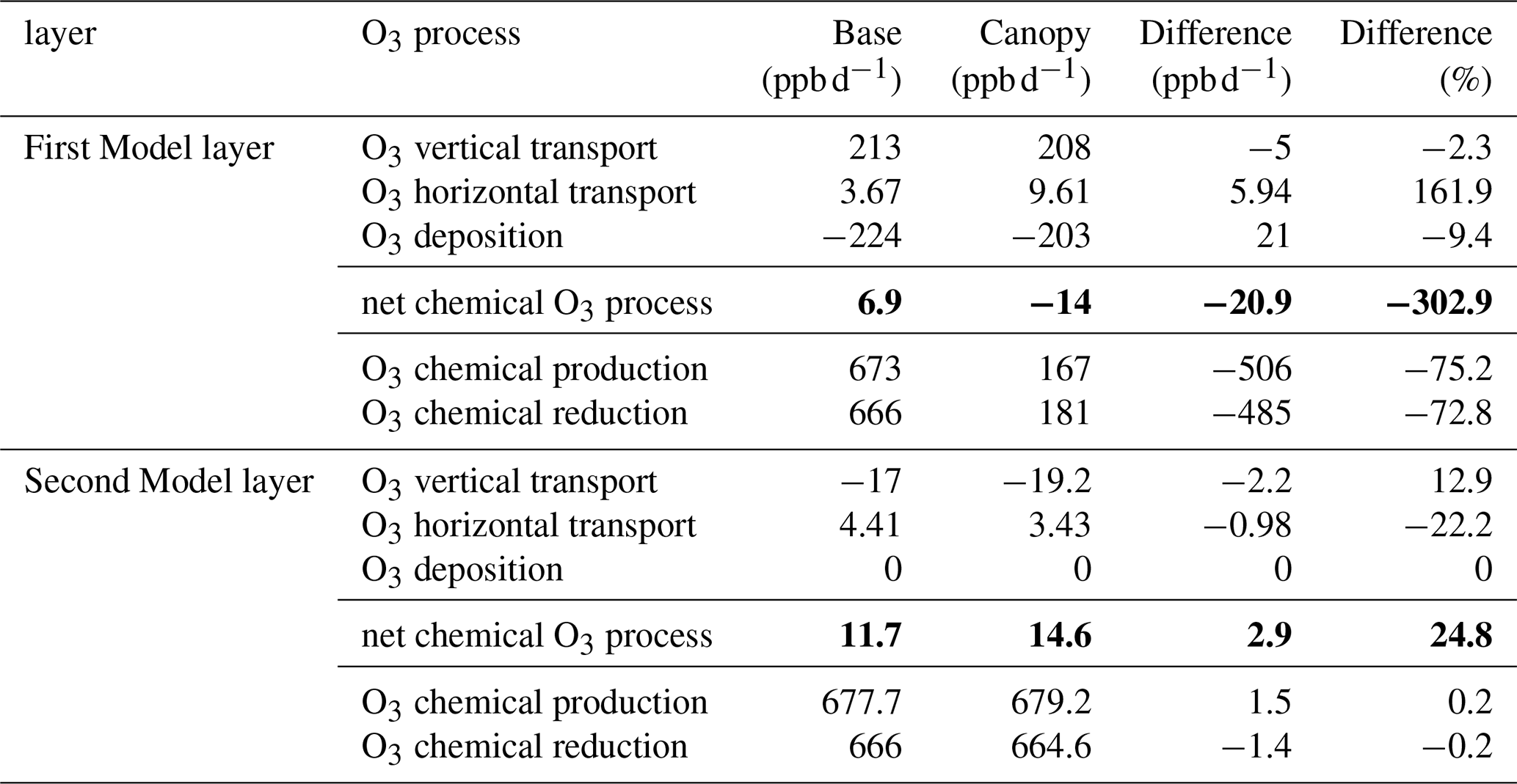
Table 3 First and Second layer O₃ PA results for Base and Canopy scenario 1 month average daily total processing rates. The bold font values represent ozone net production from all chemical reactions in CB6r3.

3.3 Process analysis and integrated reaction rate result summary for O₃, NO_x and VOC reactions

Overall, the daily total canopy runs result in net reductions of first model layer O₃ chemical formation rates (−21 ppb d⁻¹, −303 %) and vertical transport rate (−5 ppb d⁻¹, −2.3 %). The canopy leads to increases in chemical formation rates (2.9 ppb d⁻¹, +24.8 %) in the second model layer (Table 3). The canopy results in large reductions in photolysis, less NO₂ → NO conversion, enhanced NO transformation to NO₂ in the first model layer, and consequently more NO₂ transported into the second layer during daytime hours. This process increases the second layer O₃ production rates (+ 1.5 ppb d⁻¹) and reduces O₃ consumption rates (−1.4 ppb d⁻¹). These two factors cause the net second layer O₃ monthly average chemical processing rate to increase of 2.9 ppb h⁻¹ (+24.8 %). Table S1 in the Supplement shows the daytime (6 AM to 6 PM LT) and nighttime (6 PM to 6 AM LT) O₃ process rate details.

Table 4 The average daily total NO_x chemical cycle process, and net all processing rates on surface and second layer at canopy effect regions (see Fig. 2). The bold font values represent summary of major NO_x chemical reactions in CB6r3.

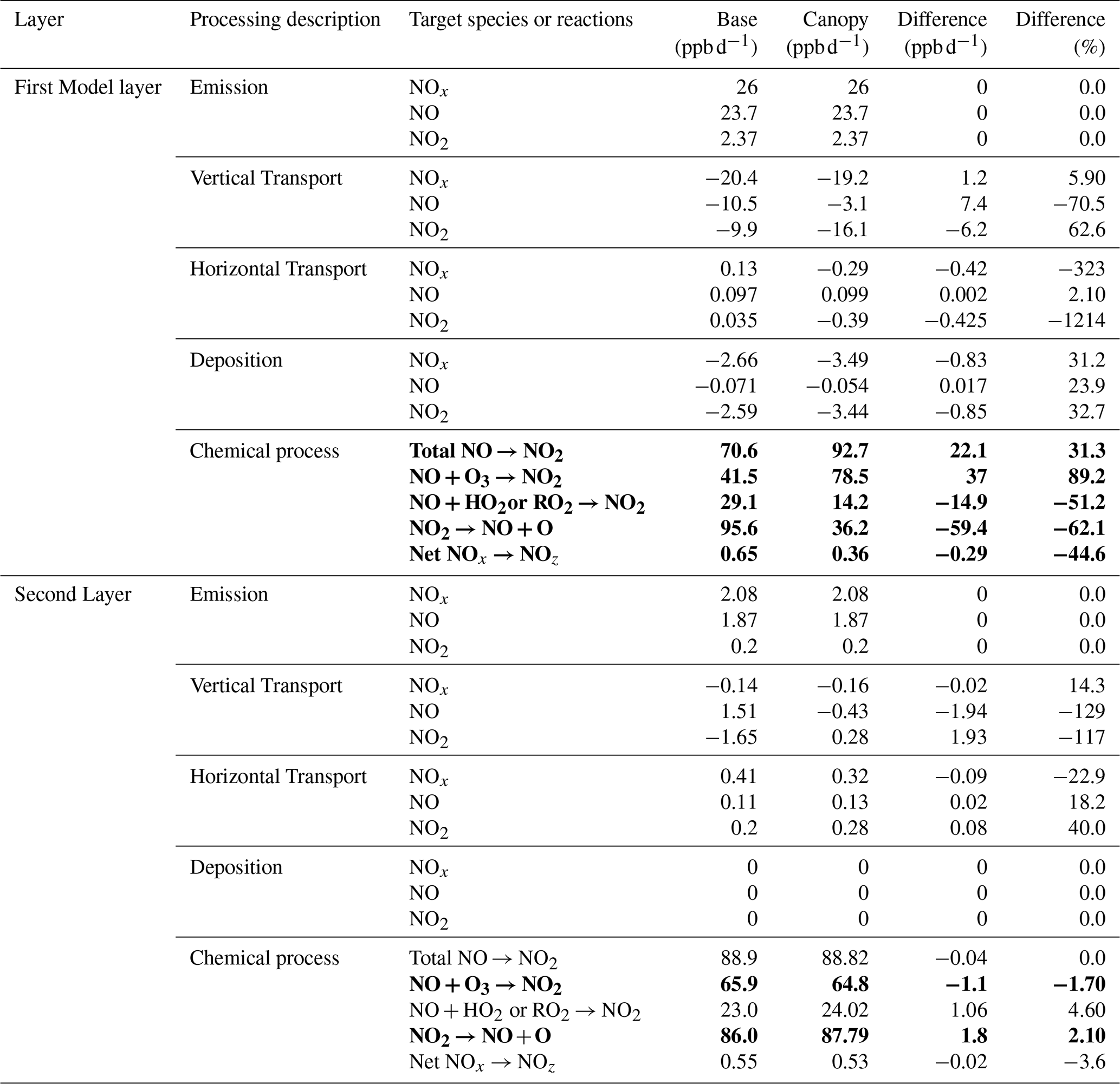
Table 5 The average daily total O_x (O₃ + NO₂) for all processing rates on surface and second layer at canopy effect regions (see Fig. 2).

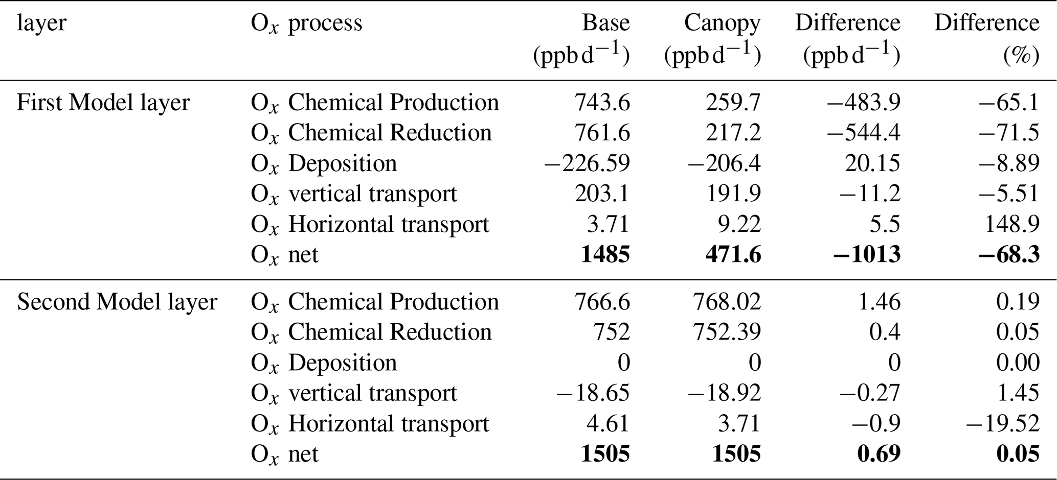
Table 6 The average daily total IRR results of new HO_x (OH and HO₂) and VOC oxidation reactions on surface and second layer at canopy effect regions (see Fig. 2).

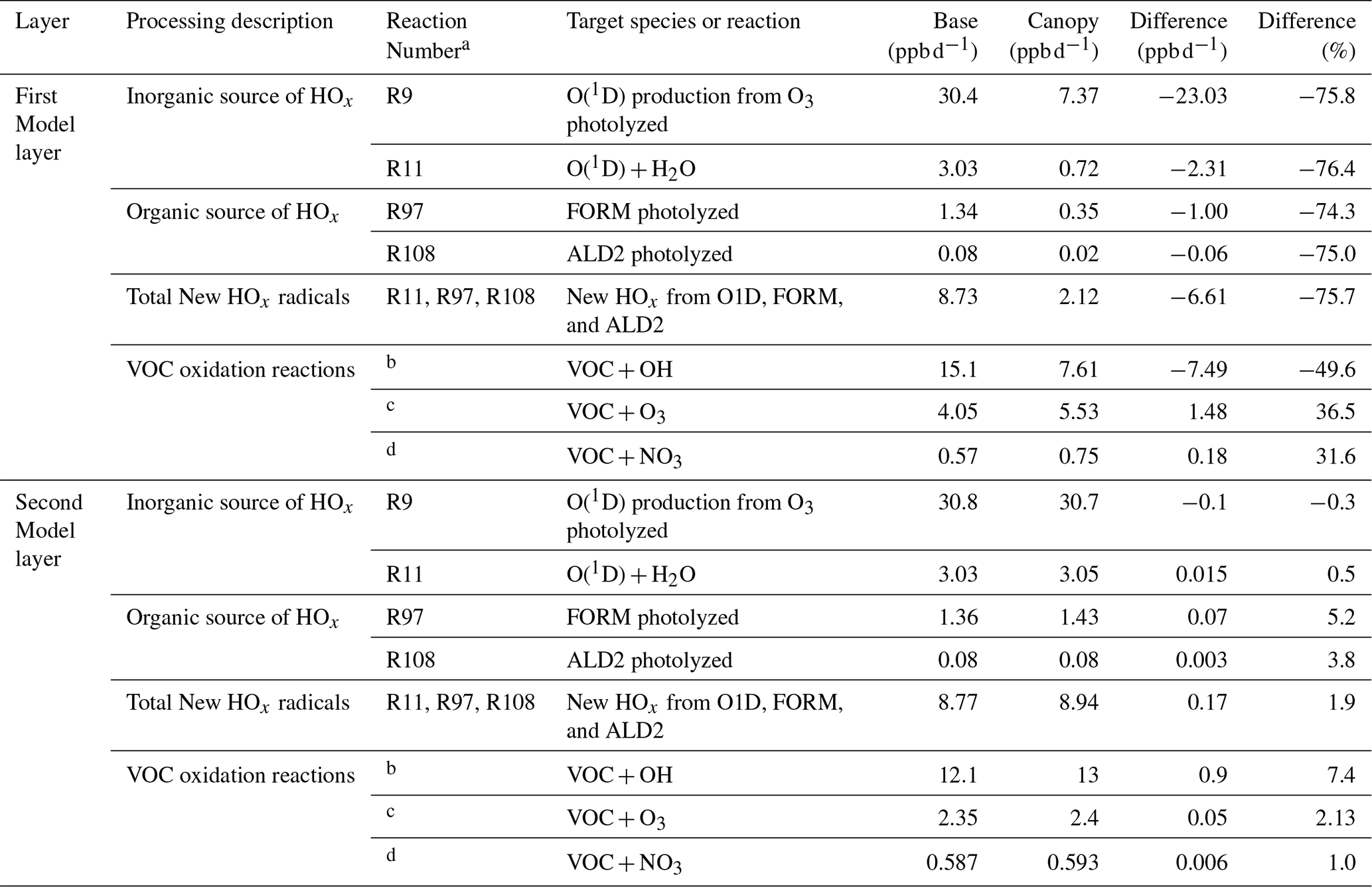
^a CB6r3 Reaction Number reference can be found: https://github.com/USEPA/CMAQ/blob/main/CCTM/src/MECHS/cb6r3_ae7_aq/mech_cb6r3_ae7_aq.def (last access: 3 November 2025). ^b VOC + OH reactions include: R106, R110, R113, R116, R121, R_125, R126, R127, R130, R131, R132, R138, R142, R146, R149, R158, R165, R170, R172, R180, R185, R186, R191, R199, R203, R206. ^c VOC + O₃ reactions include: R139, R143, R147, R156, R159, R173, R200, R204. ^d VOC + NO₃ reactions include: R107, R111, R115, R118, R120, R140, R144, R148, R157, R160, R164, R174, R192, R201, R205, R207.

Table 4 shows the NO_x processing rates and IRR results for the first and second layers to help explain the O₃ chemical process changes. The first model layer NO_x chemical processing shows that the total NO to NO₂ process increases by about 22.1 ppb (31.2 %). The changes of NO reaction processes due to the canopy include a net (1) increase in the NO + O₃ titration reaction from 41.5 to 78.5 ppb (+89.2 %), (2) decrease in NO + RO₂ reaction from 29.1 to 14.2 ppb (−51.2 %), and (3) decrease in the NO₂ photolysis process (NO₂ → O + NO) from 95.6 to 36.2 ppb (−62.1 %). Hence, the NO_x cycle was changed and overall net O₃ chemical processes become negative in the first model layer (Table 3; from 6.9 to −14 ppb, −302.9 %). This results in an increase in the first model layer NO₂ vertical transport loss (from −9.9 to −16.1 ppb, +62.6 %) and decreases the NO vertical transport loss (from −10.5 to −3.1 ppb d⁻¹, −70.5 %). Further, due to reasons described above, the second layer NO_x chemical processes have an increase in NO₂ photolysis rate (from 86 to 87.8 ppb d⁻¹, +2.1 %) and decreasing NO titration (NO + O₃) reaction (from 65.9 to 64.8 ppb d⁻¹, −1.7 %). Those NO_x balance changes cause the net chemical O₃ formation to increase about 2.9 ppb d⁻¹ in the second model layer (+24.8 %).

In addition, the canopy parameterization enhances surface removal of NO_x through dry deposition. As shown in Table 4, total NO_x deposition in the first model layer increases by 31.2 % (from 2.66 to 3.49 ppb d⁻¹), primarily due to a 32.7 % increase in NO₂ deposition (from 2.59 to 3.44 ppb d⁻¹). These results indicate that the shift in chemical partitioning toward more NO₂ formation driven by increased titration and reduced photolysis and promotes stronger NO_x removal through deposition, especially under canopy effect.

To further quantify the integrated oxidant budget in canopy-affected regions, Table 5 summarizes the average daily total O_x (O₃ + NO₂) processing rates in the first and second model layers. In the first layer, both O_x chemical production and reduction decrease substantially under the canopy scheme, by 65.1 % and 71.5 %, respectively. Dry deposition also decreases slightly (−8.9 %), while vertical and horizontal transport processes show smaller changes. The net O_x budget in the first layer decreases by 68.3 %, indicating a strong suppression of near-surface oxidant cycling under canopy influence. In contrast, the second layer shows minimal changes between the canopy and base cases. O_x chemical production and reduction remain nearly unchanged (< 0.2 %), and transport terms differ by less than ± 1 %. These results highlight that the canopy parameterization substantially affects oxidant chemistry and fate near the surface, while impacts aloft are minimal. Including the O_x budget offers a clearer picture of how chemical and physical processes are reorganized by canopy effects in the lowest layers.

In addition to the changes in the NO_x cycle caused by the canopy, the HO_x radicals (OH and HO₂) and VOC oxidation processes are significantly impacted. Table 6 summarizes the effects of the canopy on HO_x formation and VOC oxidation reactions, focusing on changes in the Integrated Reaction Rate (IRR) driven by canopy influence. The sources of “new” HO_x radicals include inorganic sources (e.g., O(¹D) + H₂O) and organic sources (e.g., photolysis of aldehyde compounds). The canopy reduces both photolysis processes, the photolysis of O₃ (O₃ → O(¹D), decreased by 75.8 %) and formaldehyde (FORM →  2HO₂, decreased by 74.3 %). These reductions greatly diminish OH radical formation and result in a 49.6 % decrease in VOC + OH reactions. Fewer OH radicals lead to reduced VOC oxidation, resulting in lower RO2 and HO2 formation. Consequently, the reactions between NO and RO2 or HO2 decrease by 51 % (Table 4). The sharp decline in OH radical formation also limits net NO_z (HNO₃ and HONO) formation processes (−45 %) in Table 4, such as NO₂ + OH → HNO₃ and NO + OH → HONO, which reduces the chemical loss of NO_x in the first layer, as indicated by the red line in Fig. 10b and c.

While VOC + OH reactions experience a significant reduction (−49.6 %) in Table 6, VOC oxidation reactions with O₃ in the first layer show an increase (+36.5 %), with reaction rates rising by 1.48 ppb d⁻¹. This increase is attributed to the reduced OH radical levels and O₃ photolysis rate in the first layer, which creates more opportunities for VOCs to react with O₃. Notable increases are observed in isoprene (from 0.56 to 1.23 ppb d⁻¹, + 120 %), monoterpenes (from 1.18 to 1.48 ppb d⁻¹, + 25.4 %), and other alkenes (from 2 to 2.51 ppb d⁻¹, +25.5 %) (see Table S2). In the second layer, changes remain minimal, only VOC + OH reactions increase slightly by 7.4 %, +0.9 ppb d⁻¹. The changes in VOC + NO₃ reactions are also negligible, with rate changes contribution below 3 % (0.18 of 6.0 ppb d⁻¹) in first layer and 0.7 % (0.006 of 0.95 ppb d⁻¹) in second layer. This chemistry and advection-driven pooling of biogenic VOCs within the canopy has been seen in observations and in high resolution 1-D canopy models in the past (Makar et al., 1999); differences in reactivity of the VOCs can lead to underestimates of the most reactive VOCs relative to those generated in the absence of chemical losses with the “big-leaf” model framework.

4 Conclusion and discussion

In this work, we implemented explicit vegetative canopy data and efficient parameterizations (Eqs. 1–3 above following Makar et al., 2017) for the effects of forest shading on photolysis attenuation and canopy-modulated turbulence (i.e., eddy diffusivities) into the widely used CMAQ model. We adopted a simplified approach, which implements the parameterization within CMAQ's existing layer structure, rather than locally adding additional layers explicitly into canopy grid cells, by weighting the sub vertical grid scale photolysis rates and diffusivities by reduction factors to account for the light and turbulence structure within the canopy portion of the model layers. We comprehensively analyzed and quantified the impacts of the canopy data and parameterizations on boundary layer O₃ predictions using CMAQ-Process Analysis (CMAQ-PA). To our knowledge, this work using the PA method is the first to detail and quantify the different roles of dynamics, physical, and chemical processes due to the presence of forest canopies on O₃.

Overall, the O₃ concentration is directly impacted at the canopy effect locations in the model. The canopy effect improves the model performance (mean bias from +0.70 to −0.10 ppb and fractional bias from +9.71 % to +6.37 %) for hourly O₃, especially in the morning hours (e.g., 7–11 AM LT). The PA results show substantial changes in the O₃ chemical process rate, both in sign and magnitude (net chemical process from +6.9 to −14 ppb d⁻¹, a −303 % change), while also altering the gas chemistry and partitioning of other NO_x, HO_x, and VOC oxidation reactions. The canopy leads to strong reductions in the photolysis of NO₂, O₃ and formaldehyde in the first model layer, which not only decreases the NO₂ photolysis rate (−62.1 %) but also significantly reduces the OH radical formation rate (−75 %) from both inorganic (O(¹D)) and organic (formaldehyde) pathways. These changes result in a −49.6 % decrease in OH-initiated VOC oxidation reactions, while increasing the VOC + O₃ reactions (+36.5 %). Furthermore, enhanced trapping NO_x and the conversion of NO to NO₂ by the canopy in the first model layer consequently leads to higher NO₂ photolysis and lower NO titration in the second layer. This causes an overall increase in net O₃ daily total chemical processing rate in the second layer (monthly average ∼ 2.9 ppb d⁻¹ or +24 %).

Altered O₃ concentration gradients due to the canopy (e.g., increased gradient between first and second but decreased gradient between second and third layers) leads to an enhanced but delayed (between about 6–8 a.m.) effect of downward transport of ozone from the second to the first model layer. Overall, the complex chemical and physical diffusion processes induced by the canopy effect reduce first model layer (near-surface) O₃ concentrations (see black lines in Fig. 7a), while increasing O₃ concentrations in the subsequent layers typically found above canopy top, and most predominantly during the nighttime through morning hours in the second layer (see black lines in Fig. 9a).

Our results of the impacts of sub-canopy parameterizations in CMAQ compare well with past work implementing a similar, but more explicit multi-sublayer methodology in the Global Environmental Multiscale-Modeling Air quality and CHemistry (GEM-MACH) model (Makar et al., 2017). Both our parameterizations and the work of Makar et al. (2017) show a similar reduction of the mean bias (MB) of more than 50 % compared to near-surface, CONUS-wide O₃ observations. Our work, however, further emphasizes the differences between CONUS-wide and “canopy-effect” locations, as well as the even larger impact of the canopy on near-surface O₃ fractional biases (FB), which representing the difference between normalized observational and modeled data (i.e., less sensitive to scale or range in data values).

There are, however, some inherent uncertainties in this study that can be addressed in the future. Notably, the impacts of the canopy parameterizations are dampened by the relatively coarse thickness of the first model layer (∼ 40 m) in the CMAQ configuration employed (Sect. 2.3), which is consistently larger (significantly in some cases) than forest canopy heights across the US (Fig. 1). This dilutes the in-canopy photolysis and diffusivity effects when integrated to obtain a “best value” within the first layer of the meteorological model layer structure currently resolved by our CMAQ implementation.

In addition, the current implementation does not explicitly represent the enhancement in vertical mixing near the canopy top due to shear-driven eddies, which are often observed in the roughness sublayer. Based on typical values of vorticity thickness and mixing length scales near the canopy top (Harman and Finnigan, 2007), we estimate that neglecting this enhanced mixing could lead to an underestimation of vertical diffusivity K_canvalue in the first model layer (∼ 0–40 m above surface) by approximately +2.5 % to +5 % under unstable conditions (late morning to afternoon), and by +10 % to +20 % under stable conditions (evening and early morning). This could partially affect simulated O₃ profiles by modulating the vertical exchange between canopy and above-canopy air. Additional details on this uncertainty estimate are provided in the Supplement (Fig. S4). In the future, the use of the multi-sublayer method (Makar et al., 2017) to improve vertical resolution could better reflect the details of the vertical structure of the canopy and further improve predictions of O₃ in CMAQ.

Nevertheless, the implementation here shows that relatively simple sub-canopy parameterizations for canopy shading and turbulence lead to improvements in CMAQ's O₃ performance, underscoring the importance of including these processes and supporting canopy data in CTMs to improve predictions of regional ozone chemistry. Further quantifying the effects of these sub-canopy parameterizations and using the robust CMAQ-PA results both quantifies and advances our understanding of the critical dynamical, physical, and chemical processes imparted by dense forest canopies, and emphasizes the need for their continued development in CTMs for both operational and community research applications. Overall, the inclusion of sub-canopy effects and their complex interactions challenge our fundamental understanding of the atmospheric state, in which the current suite of CTM and numerical weather prediction (NWP) models do not account for such interactions and rely on similarity theory and purely “big-leaf” approaches to describe the effects of dense forest canopies on such processes. As noted in Makar et al. (2017), impacts of forest shading and turbulence have similar or greater influence on near-surface ozone levels compared to climate change and current emissions policy scenarios. Thus, our work here further supports and demonstrates the importance of inclusion of such processes (even as relatively simple parameterizations) for the future of CTM, NWP, climate, and host of related Earth system models used to study the coupled atmosphere-biosphere interactions important for a myriad of applications.