The ice supersaturation biases limiting contrail modelling are structured around extratropical depressions

Contrails are ice clouds formed along aircraft flight tracks, responsible for much of aviation's climate warming impact. Ice-supersaturated regions (ISSRs) provide conditions where contrail ice crystals can persist, but meteorological models often mispredict their occurrence, limiting contrail modelling. This deficiency is often treated by applying local humidity corrections. However, model performance is also affected by synoptic conditions (such as extratropical depressions).

Here, composites of ERA5 reanalysis data around North Atlantic extratropical depressions enable a link between their structure and ISSR modelling. ISSRs are structured by these systems: at flight levels, ISSRs occur less frequently in the dry intrusion – descending upper-tropospheric air – than above warm conveyors – where air is lifted. Both ERA5 reanalysis and in situ aircraft observations show this contrast, demonstrating that the model reproduces the fundamental relationship. Individual-ISSR modelling performance (quantified using interpretable metrics) is also structured. Of the rare ISSRs diagnosed in the location associated with the dry intrusion, fewer are confirmed by in situ observations (20 %–25 % precision drop compared to the warm conveyor) and fewer of those observed were diagnosed (13 %–19 % recall drop). Scaling humidity beyond the occurrence rate bias dramatically increases the recall at low precision cost, demonstrating the potential value of scaling approaches designed with different intentions. However, the failure of scaling to improve precision, or the performance in the dry intrusion, implies that there is a need to account for the synoptic weather situation and structure in order to improve ISSR forecasts in support of mitigating aviation's climate impact.

1 Introduction

Contrails (ice clouds that form from the exhaust of aircraft) cause a significant fraction of the warming radiative forcing due to aviation (Lee et al., 2021), although they potentially have significantly less impact on climate (Bickel et al., 2025). These clouds form when the environment is below a critical temperature (the so-called Schmidt–Appleman formation criteria for liquid water supersaturation while mixing; Schumann, 1996). The initial liquid droplets rapidly freeze (as the critical temperatures are well below relevant freezing temperatures), and the resulting ice cloud evolves according to the ambient conditions.

Contrails can be “persistent”, where they continue to evolve for up to several hours, spreading and shearing beyond the aircraft's wake, often becoming difficult to distinguish from natural cirrus. The key condition for contrails to persist in the short term after formation is that the ice crystals are stable in the ambient air. For this, the ambient Relative Humidity with respect to ice (RHi) needs to be ≥ 100 %, that is, the contrail needs to form in an ice-supersaturated region (ISSR). Contrails are then broadly subject to the processes that determine the evolution and longevity of any cloud: ice uptake from the surroundings, particle losses, entrainment/mixing, and changing surrounding meteorological conditions.

These formation and persistence conditions have been shown to be consistent with observations of contrails (Schumann et al., 2017), so provide a basis for models to assess the impact of individual aircraft. However, Gierens et al. (2020) show that the ability to predict the formation and persistence of specific contrails is limited by errors in modelling ISSRs in the upper troposphere, where most planes fly. Satellite monitoring and validation are still in the early stages and can detect at most 46 % of contrails, based on the understood distribution of contrail properties from a modelled population (Driver et al., 2025). As a result, these methods alone aren't a suitable alternative for assessing the impact on a flight-by-flight basis. Therefore, accurate simulation of individual contrails is a key component of any impact assessment aiming to treat individual flights. To enable this, the biases in meteorological data need to be characterised, allowing them to be resolved, and existing data to be used effectively for evaluating contrail models (and not be restricted to an evaluation of the underlying meteorological data instead).

An understanding of how the current atmospheric state enables contrail formation, persistence, and impact is also important in order to direct mitigation activities for flights which would generate contrails with a warming impact, such as re-routing around “avoidance regions”, largely defined by ISSRs. Model studies find that applying small vertical deviations yields a significant reduction in impact (Teoh et al., 2020), and trials establish the operational feasibility (Sausen et al., 2023; Sonabend-W et al., 2024). It is important to interpret the meteorological data used to plan these activities in a way that enables successful outcomes and builds confidence.

To model contrail persistence, RHi estimates are taken from model data, including both forecast models (such as the European Centre for Medium-range Weather Forecasts' (ECMWF's) Integrated Forecast System (IFS)) or reanalysis data (when forward-looking data is not needed). Reanalysis data (such as ERA5; Hersbach et al., 2020) aims to represent the state of the atmosphere based on observations assimilated into a reanalysis model. These sources are commonly used for “offline” contrail modelling studies (when they are run separately from the meteorological model) (Teoh et al., 2022; Engberg et al., 2025).

Few observations of humidity are available to assimilate in the upper troposphere to inform the reanalysis meteorology. This means that humidity values in this region are particularly poorly constrained – Hersbach et al. (2020) show 12 %–25 % percentage-errors in the humidity, based on the ensemble spread (i.e. within 10 model realisations, each of which would be consistent with the observation and their associated uncertainty). This lack of constraint limits contrail modelling; Gierens et al. (2020) conclude that the lack of, and underestimated “degree” of supersaturation to ice are the key obstacles to modelling contrail persistence. Supporting this claim, the distribution of ERA5 RHi within ISSRs has been repeatedly shown to exhibit a dry bias compared to measurements made in situ, both by aircraft (such as the In-service Aircraft for a Global Observing System – IAGOS; Petzold et al., 2015; Boulanger et al., 2018; Gierens et al., 2020; Teoh et al., 2022; Thompson et al., 2024; Wolf et al., 2025), and radiosondes (Agarwal et al., 2022; Thompson et al., 2024).

Some progress has already been made to determine the origin of this model deficiency in ISSR diagnosis. Thompson et al. (2024) analysed the frequency and spatial distribution of ISSRs, and the degree of supersaturation within them, comparing output from forecast models to in situ observations from radiosondes and aircraft. Overactive “saturation adjustment” parameterisation (assuming all excess water vapour above saturation in clouds is frozen onto crystals) was identified as a key driver of biases limiting the frequency and degree of supersaturation. Modelling approaches designed to avoid such a parameterisation are uncommon, but are able to capture decaying ISSRs shortly after cirrus formation, and ISSRs in slowly-rising warm air that continue to be sustained even as clouds form (Sperber and Gierens, 2023).

The frequency of ISSRs in model data, and the distribution of humidity within them, can be adjusted by scaling the RHi to best match the population statistics of observed ISSRs (discussed further in Sect. 3.2, Teoh et al., 2022, 2024a; Wolf et al., 2025) . This approach may be enough to model a population of contrails for climate impact assessment or for statistical analysis of contrail properties. However, accurate ISSR occurrence rates without capturing their spatial structure are insufficient to model individual contrails more accurately, which is required for model validation or to isolate the impact of individual aircraft (as may be required for a contrail mitigation programme; Molloy et al., 2022).

One similarity between all of the aforementioned “humidity corrections” is that they are applied locally, based only on the conditions at the point of their application, this neglects the influence that dynamics has on the processes leading to ISSRs. The need to account for this structure is demonstrated by the relative success of the novel humidity correction approach taken by (Wang et al., 2025), where humidity is corrected based on both the current and past conditions both local to and in the immediate proximity to each point. However, there is structure to the weather, which shapes the formation and occurrence of ISSRs. For example, at extratropical latitudes, day-to-day variability is caused by low pressure systems, which are also called extratropical depressions, or just “lows” (Barry and Chorley, 2009). Air in different parts of the systems has different origins, and has undergone different development. The so-called “dry intrusion” that descends from near the tropopause is typically much drier than the lower-level air flows: the warm and cold conveyor belts (Browning, 1997). By averaging across many systems into “composites”, model data (including ERA5 and past reanalyses) have been shown to capture these structures (Catto et al., 2010; Priestley and Catto, 2022).

The dynamical regimes around these systems enable ISSRs to be formed and sustained, including after the formation of contrail ice. This has been demonstrated, for example, by Kästner et al. (1999), where the warm, slowly lifted air in warm conveyors, and the cold, rapidly moving air in jet streams created conditions that enhanced the rate at which persistent contrails were observed. Model biases (where an output quantity is systematically wrong) can stem from a failure to capture these underling mechanisms. Therefore, the ISSR biases ought to differ in different parts of atmospheric structures, where they are caused by different processes. These biases, a product of compounded “process errors”, are different from uncertainties in timing/the shape of the structures themselves (which are a product of uncertainties in the boundary conditions) – an ensemble approach might be suited to resolve the latter, but not the former, which can lead to model overconfidence. For example, the saturation adjustment is applied in models when clouds form (Thompson et al., 2024; Sperber and Gierens, 2023), so a dry bias resulting from overactivity in this parameterisation would be structured.

In this work, the modelling of ISSRs' spatial distribution is investigated by examining the behaviour and performance of ISSR diagnosis around weather systems using ERA5. The structures relevant for ISSR prediction should be identified, and the behaviour of ISSRs, flights, and contrails examined within them. ERA5 performance should be assessed along operational flight routes within these structures and priority areas for weather model improvements to support mitigation of contrail climate impact identified. Finally, the utility of existing model data should be explored – its impact and interpretation for applications of contrail science should be interpreted. Sect. 2 motivates the use of low pressure systems as an opportunity to explore ISSR behaviour and modelling skill. Sect. 3 introduces the methodology employed in this study: using composites to draw out the structure of the systems (Sect. 3.1) and exploration of the consequence of humidity scaling (Sect. 3.2). Then, in Sect. 4, composites reveal the structure these systems impart on a range of datasets: including ISSRs in ERA5 output (Sect. 4.1), and contrail-forming air traffic (Sect. 4.2). The structure is also explored in composites of in situ observations (Sect. 4.3), which enables the performance in diagnosing specific ISSRs be assessed (Sect. 5) and provides insight into the context where this bias develops. Finally, the applicability and consequences of these results are discussed in Sect. 6.

2 Low pressure systems – structuring the weather where contrails happen

The North Atlantic was identified as a target region to study ISSRs. A significant amount of air traffic crosses the North Atlantic every day. In 2019, this region contained 4.9 % of the global distance travelled, with air traffic density 0.03 km flown, per km² surface area, per hour, compared to a global average 0.014 $\mathrm{km}{\mathrm{km}}^{-\mathrm{2}}{\mathrm{h}}^{-\mathrm{1}}$ and peak of 0.152 $\mathrm{km}{\mathrm{km}}^{-\mathrm{2}}{\mathrm{h}}^{-\mathrm{1}}$ over Europe (Teoh et al., 2024b). This same region accounted for 10.2 % of the modelled global persistent contrail length (Teoh et al., 2024a). The contrast between the region's share of flight distance and its share of contrail length reflects that the conditions for sustaining contrails occur particularly frequently where planes fly in this region. The North Atlantic has the greatest length of persistent contrails formed per distance flown of the regions chosen in Teoh et al. (2024a). Additionally, using an ocean region for this study minimises the influence of surface inhomogeneities on weather systems – to enable the structure of weather systems to be resolved as clearly as possible. Petzold et al. (2020) demonstrate enhanced ISSR occurrence in this region compared to land regions, a result of the structure that the ocean region enables to develop. In this study, a slightly different region definition to that of Teoh et al. (2022, 2024a) was used: 20–70° N and −100–0° E.

Low pressure systems are a central feature of the weather in the North Atlantic, accounting for a significant amount of mid-latitude weather (Barry and Chorley, 2009). Understanding of these systems was developed over the twentieth century: from the processes in competing air masses at weather fronts (Bjerknes, 1919) and the “Norwegian cyclone model” (Bjerknes and Solberg, 1922), to the development of a “conveyor belt” model providing these masses at an extratropical cyclone (Harrold, 1973), to emphasising the “dry intrusion” of downwelling air from the upper troposphere (Browning, 1997). Algorithms such as that of Hodges (1999) enabled the tracking of features including these extratropical storms (Hoskins and Hodges, 2002). By compositing data at these cyclones, the features in the structure can be examined; this is particularly successful with modelled meteorological and satellite data, where spatially dense data is available (e.g. Petterssen et al., 1962; Field and Wood, 2007; Bengtsson et al., 2009; Catto et al., 2010; Priestley and Catto, 2022).

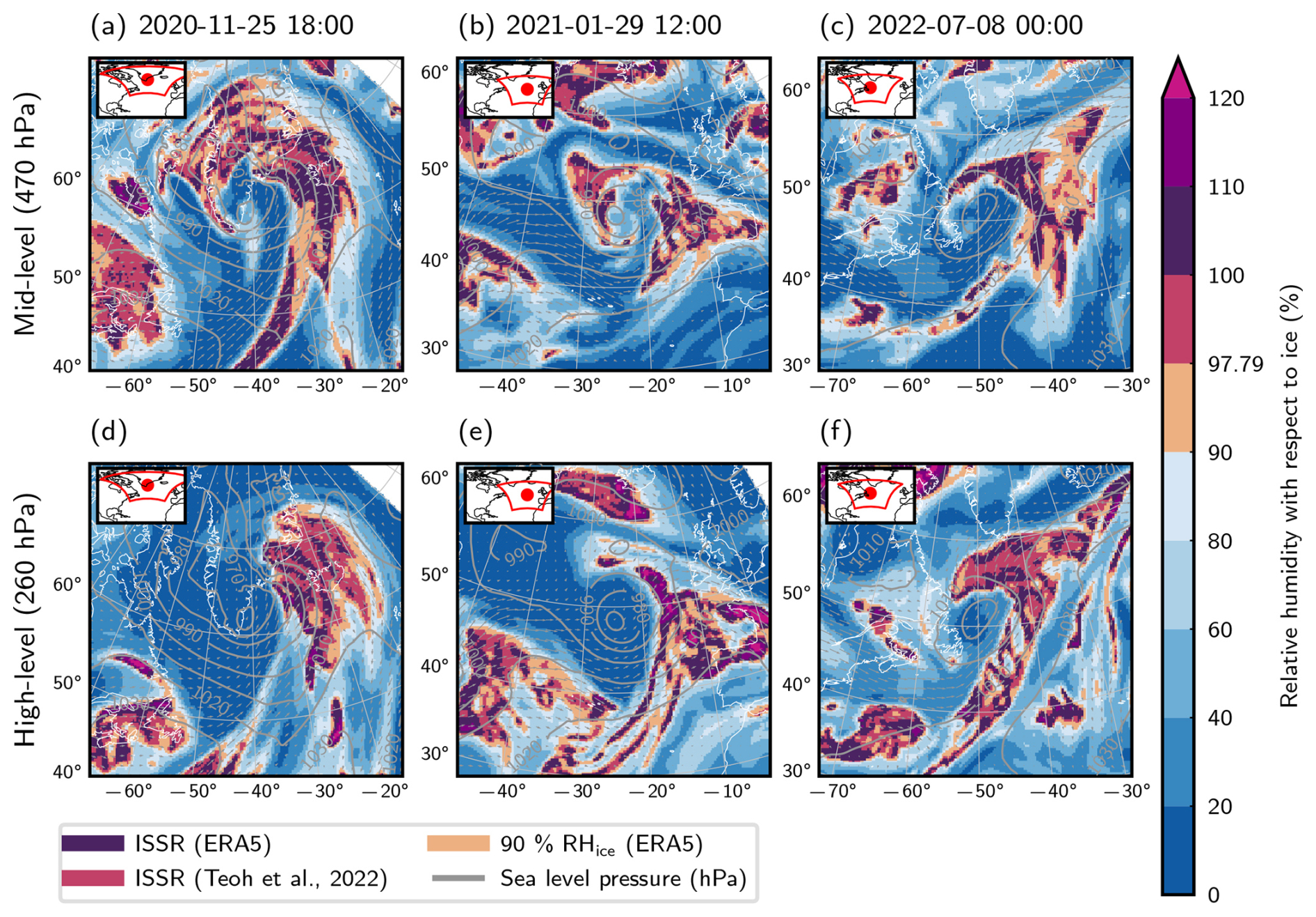
Figure 1 Charts showing the ERA5 reanalysis model meteorology around a sample of low pressure systems in the North Atlantic. ERA5 wind orientation and speed are indicated by arrows, and grey contours indicate the mean sea level pressure in hPa. Levels at 90 %, 97.79 % and 100 % RHi are ISSRs identified when applying successively less stringent thresholds, equivalent to simple uniform humidity scalings. The ERA5 data is charted at two altitudes: (a–c) are representative of the mid-troposphere (around 470 hPa, 6 km altitude) and (d–g) the upper troposphere (around 260 hPa, 11 km altitude). Empty regions (e.g. the upper right hand corner of panels (a), (b), (d), and (e)) are 10° beyond the region of interest and have been neglected from this analysis.

At a low, air circulates cyclonically around a pressure minimum, and different air masses interact. Examples of low pressure systems (including the winds and mean sea level pressure in grey, as well as the humidity) are shown in Fig. 1. The key interacting parts of these systems are (Browning, 1997):

• The dry intrusion, consisting of air descending from near the tropopause, flowing behind and into the system.

• Air upstream of the system at a lower level than the other air masses swept cyclonically around the low moving in – the “cold conveyor belt”.

• Relatively warm air, flowing with the system, also drawn poleward around the low, ascends, and can occlude the cold conveyor belt – the “warm conveyor belts” (plural, as the belt that interacts with the system is drawn away from the main flow, sometimes significantly).

These features in the systems have been demonstrated using the compositing methods. Catto et al. (2010) showed a strong signature of these features in model data around lows composited at their strongest point along storm tracks, with the conveyor belts seen in system-relative velocity composites ahead of the low, and the dry intrusion in composites of relative humidity and descending air behind the low. Field and Wood (2007) produced composites of the precipitation and cloud structures at these systems as observed using satellites, again finding consistency with a simple “warm conveyor belt” model. In this work, the dry intrusion and contrastingly humid air under the influence of the warm conveyor (albeit at a higher level, more relevant for aviation) are examined – the corresponding regions are highlighted on relevant composites in the course of this work (e.g. Fig. 3e).

The different parts of the systems not only have different character, but have distinct histories, which mean that their state is influenced by different model processes. Wernli et al. (2016) examine the history of air parcels to classify different cirrus in reanalysis data, demonstrating the different processes leading to distinct character in different parts of the system. For example, the ice clouds associated with warm conveyor belt outflow tend to have evolved from historic liquid clouds, which is a fundamentally different process to the ice clouds which form in situ, entirely at high altitudes. The diversity of these systems, where contrasting model processes will have led to the current state, make this a compelling situation through which to examine and contrast ISSR modelling performance.

Examining individual cases, these well-characterised systems are seen to shape the patterns of ISSR occurrence (Fig. 1). The different structures around the systems provide an opportunity to contrast model representation of ice supersaturation in air which has undergone different processes. This can then act as a framework to set expectations for contrail modelling.

3 Methods

3.1 Composites of low pressure systems

Low pressure systems were identified in ERA5 reanalysis Mean Sea Level Pressure (MSLP). Low pressure systems' centres were identified as locations in ERA5 which had the lowest MSLP in a 10° square region surrounding them, where this minimum value is at least 15 hPa lower than the average over the surrounding 4000 km × 4000 km region. The three systems shown in Fig. 1 are examples of those detected. Data was then added to the composite in this (4000 km × 4000 km region around the centre of the low. The data is projected onto an orthographic co-ordinate system centred on the low. The projection is analogous to the “radial” coordinate system of Catto et al. (2010), so avoids projection-related biases. ERA5 data was composited every 6 h (00:00, 06:00, 12:00 and 18:00 UTC) for the six-year period 2018–2023 (inclusive). The spatial distribution of lows included in the composite is shown in Fig. 2. For vertically-resolved data, seven pressure levels were used, every fifth ERA5 L137 model level between levels 70 and 100 (ca. 580–160 hPa), though much of the below analysis focuses on two levels at approximately 260 and 470 hPa (“high-” and “mid-” level, respectively).

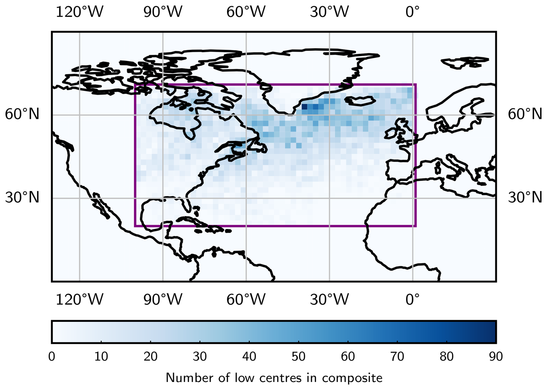
Figure 2 The distribution of low centres included in the composite.

The RHi from ERA5 is used to find modelled ISSRs. In this work, this RHi has been calculated from the specific humidity, temperature, and pressure according to the Murphy and Koop (2005) formulae for the saturation vapour pressure, valid for temperatures between 110 and 273.16 K. This approach is taken to ensure a consistent representation of RHi with temperature, rather than using the hybridised relative humidity that is provided as ERA5 output.

In this work, data was not rotated according to the direction of storm propagation – this additional step has been performed in some previous low-compositing studies. By maintaining the orientation with the cardinal directions, features which are not primarily associated with the storms can also be interpreted (such as flight data). This alignment is imposed at the centre of the systems; the projection induces some distortion away from the cardinal directions elsewhere.

To further discriminate the signal due to the system from the features due to their geography or climatology, an additional “counterfactual” composite was produced. This contains data from the same sources as the composite, at locations where lows were detected 365 d earlier. By considering this data, which is randomly distributed relative to the centre of low pressure systems, the system-relative anomalies due to the specific presence of the low can be isolated from the background variation in meteorological properties (Tippett et al., 2024). The resulting anomalies are termed the “signal” due to the low. These signals include the system-relative winds, further alleviating the need to detect storm tracks or rotate composited systems relative to system propagation.

In this work, as much data as possible was included, to enable the consideration of relatively sparse in situ observations, and make conclusions that are relevant in the “ordinary” weather where planes fly. To achieve this, all the low pressure systems detected were kept, including where these are repeated detections of the same system – we assume that no individual anomalous system overwhelms the composites produced. This approach is inherently a trade-off, no attempt has been made to isolate a particular phase of system development, instead prioritising the inclusion of as many systems as possible. Producing composites with meaningful structure acts as the test of validity for this approach. In the composites of ERA5 data, 14 076 low pressure systems were found, and 14 251 in the counterfactual (with the small variation due to different years used to detect lows for the counterfactual).

Other data was composited over subsets of the time of the ERA5 composites. Flight activity (the number of flown kilometres, per km² horizontal area, over the hour previous to the composite timestep; Teoh et al., 2024b) was added to the composites for 2019. Flight data from 2020 and 2021 was excluded to ensure normal behaviour of air traffic. Contrails modelled by Teoh et al. (2024a) using CoCiP (the Contrail Cirrus Prediction model Schumann, 2012), using the pycontrails Python library's “trajectory” implementation (Shapiro et al., 2023), were also included, based on all the flight activity in 2019 and ERA5 meteorological data with the humidity scaled. Radiative forcing estimates in the same dataset are based on Schumann et al. (2012). For these modelled contrail data, the contrail segments existent at the instant of the composite timestep are composited. Finally, IAGOS in situ observations of RHi (Boulanger et al., 2018) are added to composites where they are available (2018–2022).

3.2 Scaling and the morphology of ice-supersaturated regions

Physically, ISSRs are characterised by RHi ≥ 100 %. Due to the biases in model simulations of ISSR occurrence, different scalings to RHi have been used to improve ISSR prediction. Schumann (2012) and subsequent early CoCiP studies enhanced the frequency of ISSRs using a scaling factor (in terms of ISSR identification alone, this is equivalent to applying a lower threshold). Teoh et al. (2022) increase the frequency of ISSRs to match in situ observations (also by scaling the humidity for a reduced threshold), and spread the RHi distribution towards higher values within the ISSRs (according to a power law relationship). Teoh et al. (2024a) revised this approach to suit the needs of a global analysis, acknowledging a latitude dependence in the scaling required. Wolf et al. (2025) similarly impose the IAGOS distribution – producing a mapping based on both the modelled humidity and temperature as well as both latitudes and pressure levels (altitudes).

Each of these approaches aims to increase the frequency of ISSRs in model data to better match observations, and more recently also induce a more-accurate RHi distribution within them. Any tailoring of the corrections to the current weather are parameterised based on climatological analysis. Specifically, the treatment is based on the typical bias at a location, such as the latitude dependence in the correction of Teoh et al. (2024a), or by also considering typical behaviour of the bias based on the temperature at a given location, as in the approach taken by Wolf et al. (2025). Otherwise, changes to the spatial distribution of ISSRs are “emergent” (e.g. the morphology of ISSRs is altered by the lower effective threshold). In contrast, the actual error in the modelled humidity fields is not expected to be a purely random bias but has a strong systematic component, depending on the meteorological state and history of an air mass. Other approaches, such as the statistical modelling of persistent contrails as in the work of (Duda and Minnis, 2009a, b), have taken into account an even broader array of characteristics. But ultimately, the aforementioned approaches are all local, so don't fully account for the weather's structure. Only an approach that accounts for the dynamics, as in the recent work by Wang et al. (2025), has the potential to account for the causes of the bias.

These emergent adjustments to the spatial distribution expand ISSRs and effectively join together ISSRs into humidity filaments in the meteorological data. This behaviour can be seen in the examples of Fig. 1, showing the ISSRs identified in the ERA5 humidity. The contour levels show ISSRs identified based on different ERA5 RHi thresholds: using the physically expected threshold of 100 % on unscaled data (ERA5-native ISSRs), the Teoh et al. (2022) scaling (a “correction” to the ISSR frequency), or an even-less stringent threshold of 90 %. As the thresholds become less-restrictive, the morphology of the regions changes, from particularly fractal-edged regions that are occasionally separate from other local associated ISSRs, to large, smoother-edged regions. Some ISSR boundaries are particularly “steep” (where changing the threshold hardly moves the boundary). The steep boundaries are expected, especially at the fronts on the inner edge of the low, where the humid warm conveyor belt meets the dry intrusion. Therefore, the ISSRs diagnosed by applying a lower RHi threshold are geometrically expanded but under a conservative approach – the model knowledge of the air mass boundaries is retained. For producing composites in this work, the smoother ISSRs diagnosed while maintaining the steep boundaries have the additional advantage of reducing noise in composites, so the least-restrictive threshold shown (90 %) is used in this work unless specified.

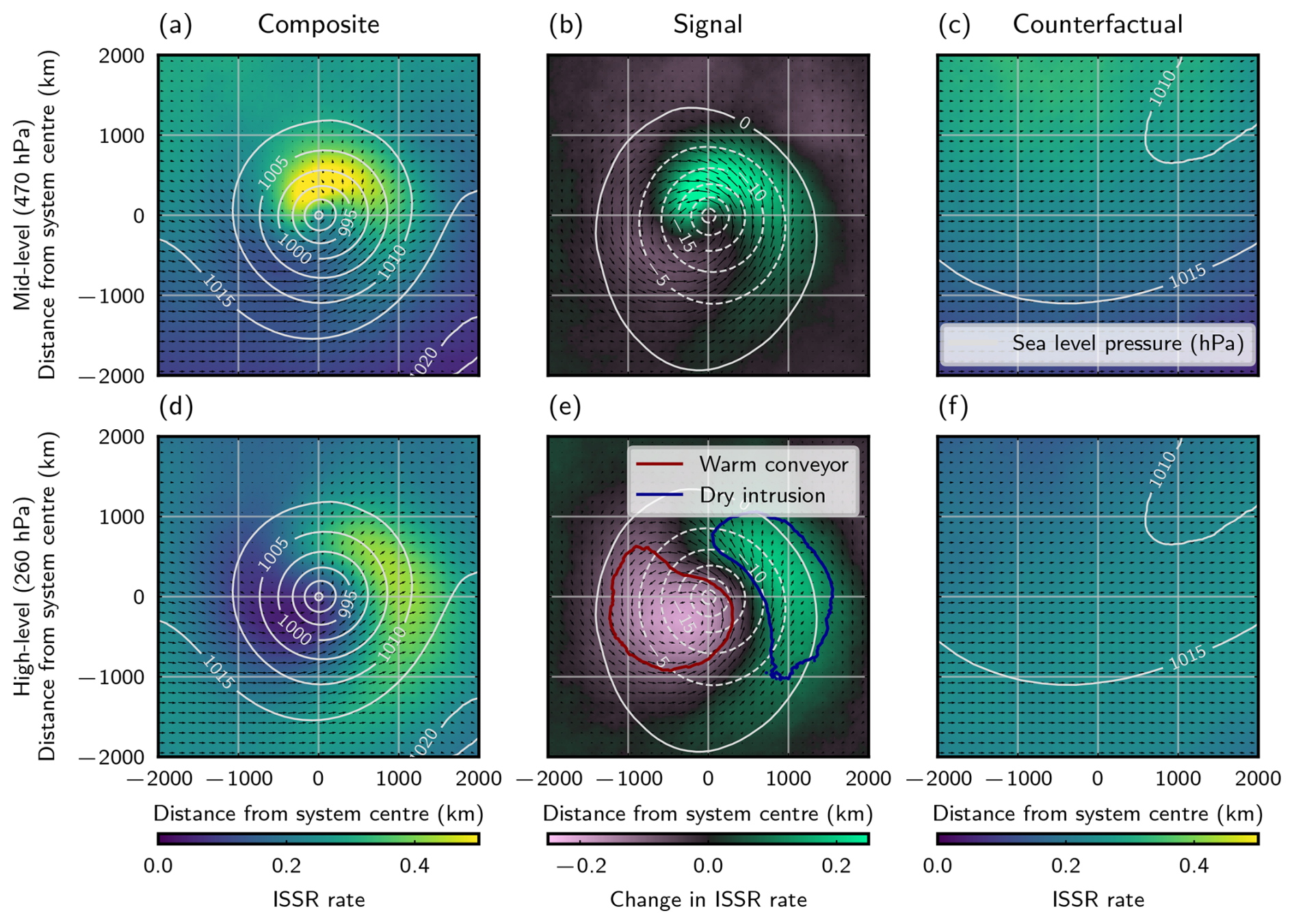
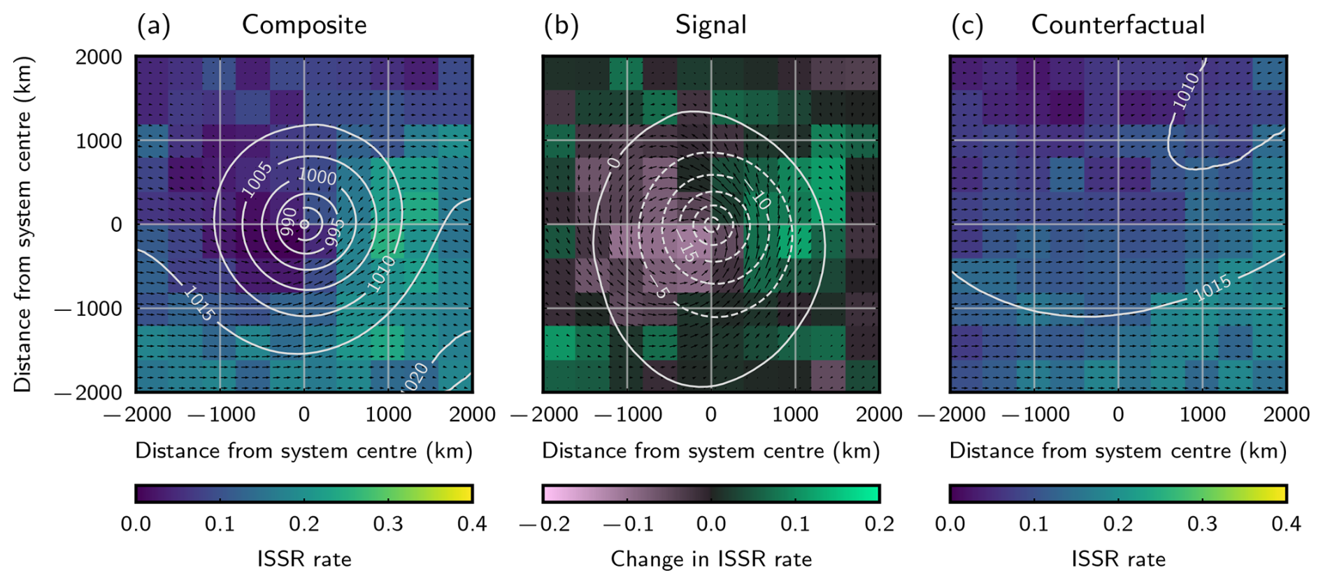
Figure 3 The mid- (a–c) and upper- (d–f) troposphere composite structure of ERA5 ISSR occurrence around locations of North Atlantic low pressure systems. The composites (a, d), show the rate at which ice-supersaturation occurs at locations relative to the centre of a low, while the counterfactual data (c, f), show the same ISSR rate occurring 365 d after a low was detected (i.e. a mean state of the meteorology, sharing the geography and seasonality of low occurrence). The “signals” (b, e), show the difference between the composite and counterfactual fields. The signal can be interpreted as the impact due to the presence of the low pressure system, or the system-relative quantity. A RHi greater than 90 % has been used to indicate modelled ISSR. The red and blue contours of panel e denote contrasting regions used for analysing ERA5 accuracy in Sect. 4.3.

4 Composites around low pressure systems

4.1 Reanalysis ice-supersaturation

The ERA5 reanalysis is seen to capture the structure of humidity within the mid- and upper-tropospheric levels of an extratropical cyclone (Fig. 3). The composites and counterfactual composites, respectively (Fig. 3a and c) show the frequency with which an ISSR occurs at a location, either around lows, or in regions sharing the location of a low that occurred 365 d earlier. This includes all ISSRs diagnosed against the threshold, including where cloud is found and where the temperature may not be low enough for a contrail to form. The signal (Fig. 3b) then highlights the change in this rate due to the presence of the low – the structure given to the system because a low pressure system occurs here.

This is in broad agreement with past work, such as Catto et al. (2010). Specifically, a dry intrusion behind the cyclone at the high level, and the comparatively-humid region above the warm conveyor belt are visible. A clear comma-shaped structure is seen at the mid-level altitude, which corresponds to the location of the cloud head (despite this being a higher level than might be typical for those features). Humid air here has been lofted in the warm conveyor belt.

To be explicit, the mid-level ISSRs should not be conflated with regions at risk of contrail occurrence, and temperatures at this level are mostly too warm for contrails to form. Instead, the mid-level composite is presented to provide context for the vertical structure, the location of lower-level clouds, and for comparison with past compositing work. The conditions for contrails, including temperature and air traffic are considered in the analysis below, where CoCiP-modelled contrails are used as a single proxy including all these factors. Although ISSR occurrence remains the useful metric in the context of this article, which characterises the ISSR occurrence rate bias, conserved quantities offer a useful point of comparison to other atmospheric physics work and provides an intuition as to the flows in the system, therefore, we provide composites of the water vapour mass mixing ratio in Appendix A.

In the high-level composites, the signature of the warm conveyor belt is positioned further from the low, moved further east by the slant of the weather front. In the north of this humid region, the structure transitions between the two levels, from the cloud head at the mid-level to follow the structure expected of the westerly jet. There is additionally a change in the behaviour of the mean-state of humidity (seen in the counterfactual): in the mid-level, supersaturation occurs less frequently towards lower latitudes, while any trend is weak at the high level (and if any exists, it is reversed). This variation in the background justifies the composite/counterfactual approach, and could otherwise contribute a bias.

It is counterintuitive that the upper-level composite shows a sweeping arc of humidity in a manner that appears cyclonic, in a part of the system where a transition to anticyclonic flow might be expected, coincident with the outflow. In fact, the nature of the flow in this part of the system is indeed anticyclonic, as demonstrated in composites of the potential vorticity, which are presented in Appendix B. This transition to anticyclonic flow is shown in outflow regions in the individual case studies (Fig. 1d–f). Ultimately, the composite winds do suffer some smoothing as a result of the trade-off made to include systems at multiple phases of their evolution, in order to consider as much data as possible.

The highly structured nature of ISSR occurrence is illustrated by the range of ISSR rates that occur, despite the number of different systems included in the study. At the location of the minimum rate in the high level composite, in the dry intrusion, ISSRs are diagnosed in only 4 % of lows, this contrasts 43 % of lows at the maximum above the warm conveyor, that is, ice supersaturation is 91 % less frequent at the dry extreme than where ISSRs are most frequent. In the counterfactual, where a low is not conditioned upon, averaged ISSR occurrence rates only vary between 14 % and 26 %, despite the significant geographical extent, highlighting the role of the low pressure system itself in generating the pattern of ISSRs.

Structure can also be seen in the horizontal winds and the MSLP (respectively the arrows and contours of Fig. 3). There is a minimum of MSLP at the composite's centre, caused entirely by the presence of the low (i.e. occurring only in the signal and not the counterfactual) – expected as this is defining the weather system for the purpose of this work. The system-relative winds have been isolated as the signal – they are velocities relative to the counterfactual mean state. Cyclonic winds are seen around a core slightly south west of the low. The cyclone trails further at high level, the system is slanted (this is a requirement for the conservation of energy).

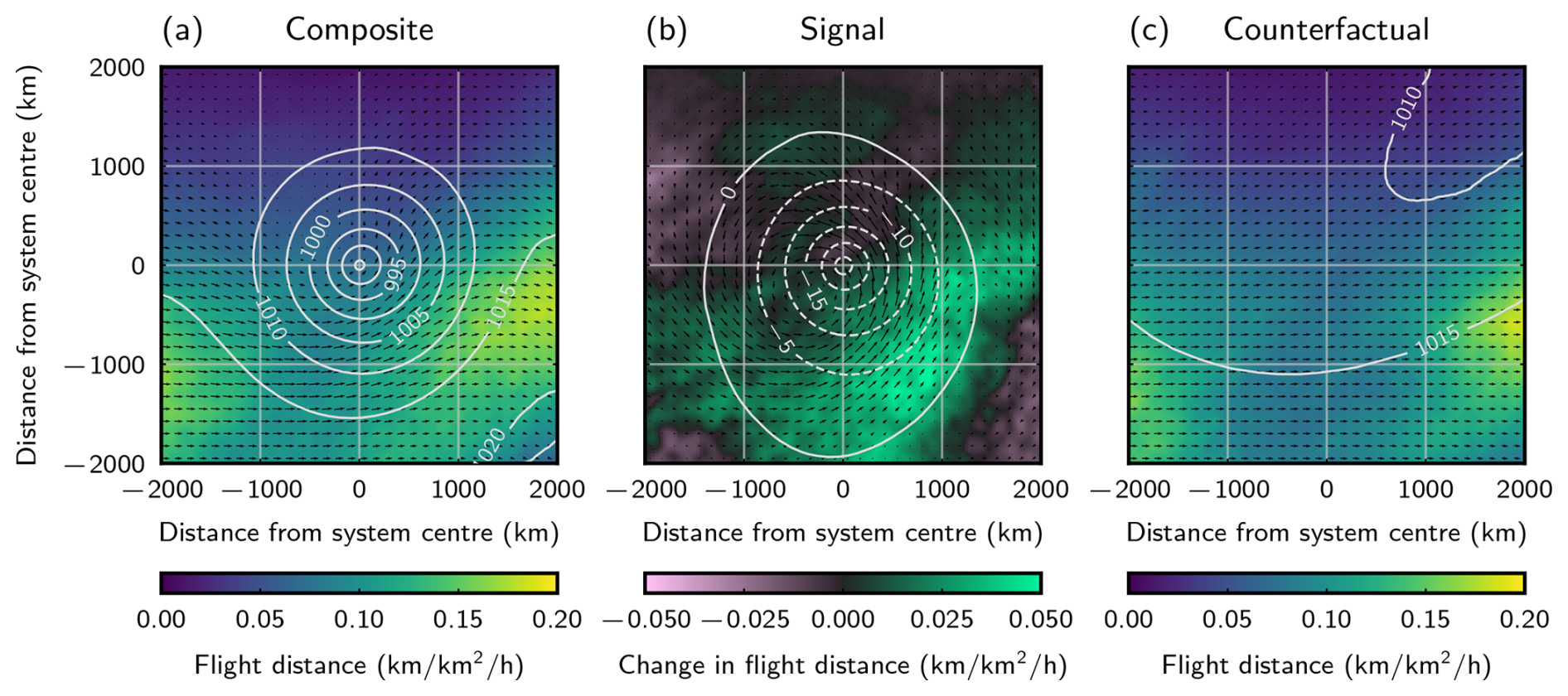
Figure 4 Composite, signal, and counterfactual (as Fig. 3) of distances flown around lows by aircraft in the GAIA dataset per unit area, per hour, based on traffic in the hour preceding the composite time (Teoh et al., 2024b). Data is integrated across the composited vertical levels.

4.2 Flight distance and contrails around storms

4.2.1 Flight distance

Air traffic in this region is concentrated between 9 and 12 km altitude (Teoh et al., 2024b), so model studies conclude that contrail formation is also concentrated around this altitude (Teoh et al., 2024a). The “high-level” of Fig. 3d–f, which corresponds to approximately 11 km altitude, is therefore the most appropriate of this study's vertical levels to represent the meteorology at aircraft cruise altitude. The structure of ISSRs observed in the high-level composites (Fig. 3d–f) can be combined with the distribution of flight distance to set expectations for the behaviour of persistent contrails.

Figure 4 shows the vertically-integrated distance flown around low pressure systems (from the GAIA inventory;  Teoh et al., 2024b). As discussed in Sect. 3.1, only data from 2019 was used. The composite and counterfactual (Fig. 4a and c) have similar structures – there are few changes to flight behaviour due to the presence of a low. This is aligned with expectation: the key determinant of the distribution of air traffic is the distribution of destinations. In the usual distribution of air traffic, most clear in the counterfactual composite, peaks are seen in air traffic in the lower left and lower right sides of the composites. These are associated with air traffic over North America and Europe.

However, a slight redistribution in the air traffic around low pressure systems is noticeable when the signal is isolated (Fig. 4b). Traffic is increased in the southern portion of the signal where the system-relative winds are westerly. This can be interpreted as routing decisions favouring strong tailwinds, especially for eastward flights which seek to minimise cost by use the North Atlantic Jet Stream to save journey time and fuel (Wells et al., 2021).

The structure present in the composites of air traffic density suggest different behaviour depending on the longitudes, strong enough to cause peaks in the total composite. The counterfactual methodology has enabled the general signal due to a low to be isolated independently, but it is useful to break down the air traffic by longitude in order to provide supporting evidence. This is presented in Appendix C.

4.2.2 Contrail formation and persistence

Persistent contrails are a product of ISSRs (Fig. 3) and air traffic (Fig. 4), but several other factors play a role, including the advecting winds, and the Schmidt–Appleman condition for formation. The distribution of CoCiP-modelled contrails around the low was analysed, because this data encompasses all of these factors affecting the distribution of persistent contrails. The data are as produced by Teoh et al. (2024a) for 2019, using ERA5 meteorology with the humidity scaled.

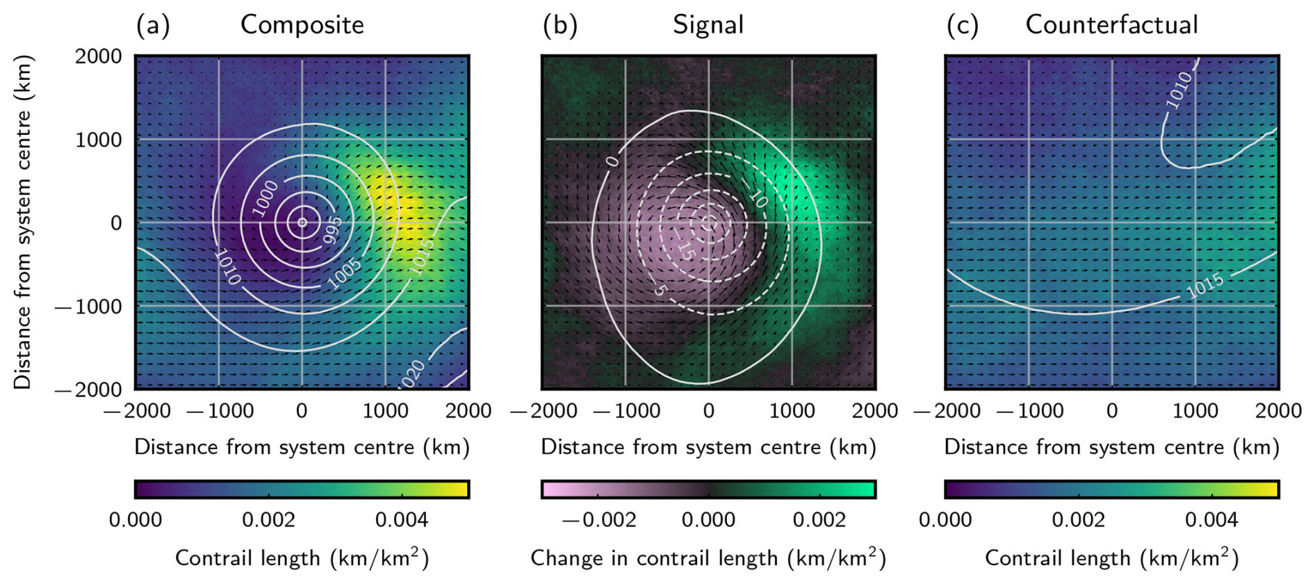
Figure 5 Composite, signal, and counterfactual (as Fig. 3) of the persisting length of contrails existing at the time of the composite per unit area. Data is integrated across the composited vertical levels so reflects contrails which exist at any altitude.

At low pressure systems, persistent contrail occurrence (Fig. 5b) shares the structure of high-level ISSR occurrence (cf. Fig. 3e). This is a perturbation to the distribution seen in the mean state (Fig. 5c), which instead broadly follows the distribution of air traffic (cf. Fig. 4c). The fact that these features are prominent in the composites of persistent contrail length indicates that none of the other factors influencing their modelling are dominating over these two most-fundamental conditions (the existence of a flight, and ambient ice-supersaturation) in the region where these systems occur.

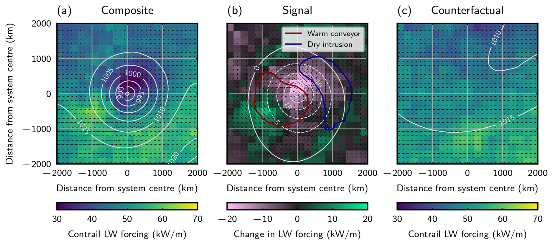
Figure 6 Composite, signal, and counterfactual (as Fig. 3) of the mean estimated instantaneous long wave radiative forcing of contrails per unit length (i.e. the relative importance of the contrails at this location for climate forcing). Data is integrated across the composited vertical levels so reflects contrails which exist at any altitude.

Not every persistent contrail has the same impact. Figure 6 shows the spatial distribution of the warming long wave component of instantaneous radiative forcing per unit length of persistent contrail that is modelled at a given location around a low. We present the long wave forcing, rather than the net forcing, because variability in incident solar radiation introduces a large component of variability shared between the counterfactual and composite, making the underlying distribution of values difficult to differentiate. Contrails tend to have a reduced impact in a region centred north east of the low (Fig. 6b). This region of reduced impact is coincident with the “cloud head” (cf. the mid-level humidity signal, a proxy for underlying clouds, Fig. 3b). Natural cirrus is likely to form here, which means that contrails are unable to contribute additional radiative effect. Conversely, there is a return to the typical contrail forcing behaviour (similar to the counterfactual) behind the low pressure system, partially co-located with the dry intrusion. It is in these parts of the system where contrails have the opportunity to exert stronger forcing when there is not a competing natural cloud radiative effect.

Figure 7 Composite, signal, and counterfactual (as Fig. 3) of the IAGOS-detected ISSR rate. The scales are chosen to match Fig. 3. Data is averaged across the composited vertical levels where IAGOS aircraft fly, so the altitude of detected ISSRs reflects that typical of operational aircraft.

4.3 Observed ice-supersaturation

ISSRs detected by IAGOS in situ ISSR measurements are composited in Fig. 7. To maximise the number of measurements, we include IAGOS observations taken at all levels. It remains appropriate to compare against the “high” altitude composite of ERA5, because this approximately corresponds to typical flight altitude (Fig. 3d–f). The structures observed in the composites are aligned with those seen in the high-altitude composite from the reanalysis model output in terms of their geography and sign, though they suffer far more noise due to the sparse measurements. The same sweeping region with a greater tendency for ice-supersaturation, associated with the warm conveyor, is seen. A prominent dry intrusion is also seen, as it was in the ERA5 composite.

Although the signs of the signal within the contrasting structures are shared between the model and ERA5-diagnosed occurrence rates, the ISSR rate in the observed composite (Fig. 7a) peaks at 25 % of systems, much less than the 43 % of systems in which ISSRs were diagnosed at the most frequent location in the ERA5 composite (Fig. 3a). This significant over-diagnosis from models is partially accounted for by the low threshold of 90 % applied to ERA5 RHi for diagnosis. Additionally, the sparse IAGOS data means that extremes are less frequently captured (e.g. the most-frequently dry region of this composite has no observed ISSRs) and the coarsening required to treat the sparse statistics causes additional smoothing of the spatial structures.

5 Evaluating diagnosis of individual ISSRs

5.1 Comparison framework

The ability to confidently diagnose specific ISSRs using the ERA5 reanalysis meteorological data is now assessed, as measured by comparing to IAGOS. To do this, the way in which the data was coarsened was refined, enabling the performance in different parts of the structure to be interpreted. Then, diagnosing ability is examined using a range of metrics, enabling the application impact to be interpreted.

In comparison to the ERA5 data, the IAGOS data is spatially sparse, so composites of this data are much noisier. Measurements are available around 2670 lows in the composite, and 2532 regions in the counterfactual. The issue of noise is exacerbated when computing classification metrics, which rely heavily on the number of supersaturated regions encountered, which make up only a small proportion of the measurements (particularly in the dry intrusion). It is necessary to aggregate larger areas (such as by coarsening the composites, as in Fig. 7) to increase statistics and reduce the impact of this noise. Instead of coarsening, introducing physically meaningful regions allows ISSR modelling performance to be compared to the distinct underlying atmospheric processes. Suitable regions were found by thresholding based on the contrasting behaviour in the ERA5 ISSR “signal”, Fig. 3e. A signal less than −0.1 was treated as the area influenced by the dry intrusion and a signal greater than 0.1 used to denote the region influenced by the warm conveyor. These regions are identified at the “high level”, which is typical for much of the air traffic and the IAGOS measurements in the region, however, data colocated with IAGOS measurements at all levels were used. The regions are chosen by their similar size and contrasting ISSR behaviour, rather than any other characteristic of these parts of a low. The regions are marked on Fig. 3e and Fig. 6b.

IAGOS measurements are frequent, approximately every 4 s during a flight, yielding an apparent spatial resolution of approximately 1 km. However, limitations of the humidity sensor at the cold temperatures expected (Neis et al., 2015) mean that ISSRs are unlikely to be resolved at this scale (Wolf et al., 2024), furthermore, this is significantly higher-resolution than ERA5. To mitigate these biases, and enable a consistent data format, IAGOS measurements have been averaged onto the same grid as the composites, including the 7 vertical levels (Sect. 3.1). The average measured humidity value for one grid box (which is approximately a 25 km square laterally) is considered a “measurement” of the ISSR status for the calculation of performance metrics. As previously, the counterfactual serves as a point of comparison – to indicate typical performance for the region, seasonality, and time of air traffic making measurements – as well as enabling the isolation of under- or overperformance as a signal due to the presence of the low.

ISSRs are treated as the “positive” case, the IAGOS measurements of ISSRs as the “truth”, and the ISSR status from the thresholded ERA5 data at the location of the measurement as a predictor. Therefore, “true positives” (TP) are IAGOS-measured ISSRs correctly identified as such when threshold is applied to ERA5 RHi, “true negatives” (TN) occur when unsaturated regions are measured by IAGOS and also predicted using the ERA5 data. False positives (FP) and false negatives (FN) occur when the IAGOS measurement differs from the ERA5 ISSR status – FP when ERA5 wrongly predicts ISSRs, FN where ISSRs were measured but weren't in the model data. ERA5 ISSR status was measured using the same three thresholds as illustrated in Fig. 1.

To assess ISSR measurement performance, we calculate binary classification metrics in these two regions, and across the composited data as a whole. We also calculate in the corresponding parts of the counterfactual – as before, this provides a point of comparison that is agnostic to the presence of a low, but shares the particular geography and seasonality of low pressure systems (and the slight differences for the location of the region). We calculate error bars by bootstrapping across 1000 samples (Efron, 1979).

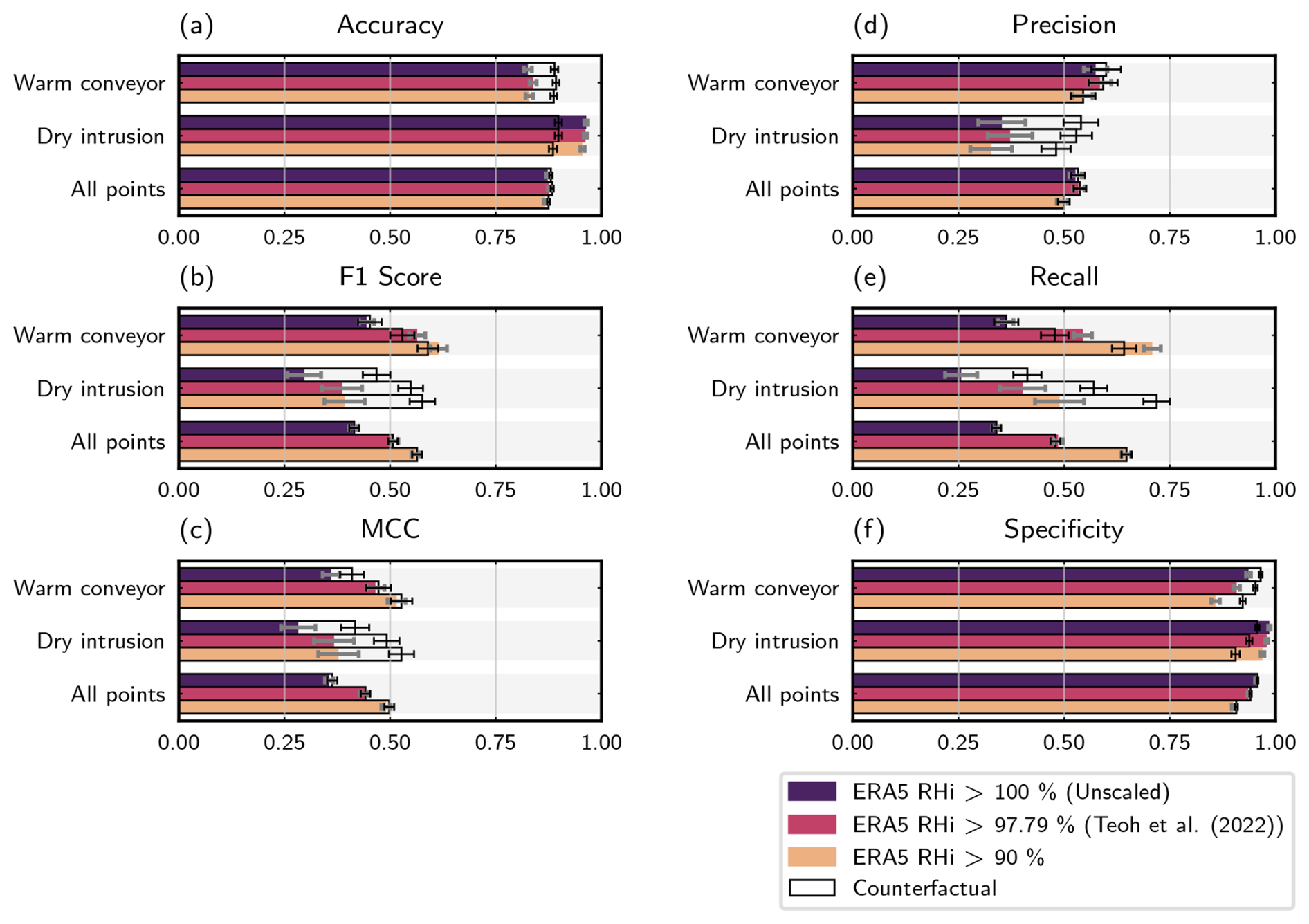
Figure 8 The ability to diagnose ISSRs detected by IAGOS using ERA5 reanalysis meteorology data in different regions around the low, quantified using accuracy, precision, recall, and specificity (a–d, respectively). Each metric is calculated using three different thresholds to define ISSRs, equivalent to applying simple scalings to the RHi. Error bars result from bootstrapping the metrics across 1000 samples with replacement.

The accuracy,

$$\begin{array}{}\text{(1)}& \text{accuracy}={\displaystyle \frac{\text{TP}+\text{TN}}{\text{TP}+\text{TN}+\text{FP}+\text{FN}}},\end{array}$$

is the proportion of measurements that are correctly captured in ERA5. Values in the dry intrusion, warm conveyor, and over the whole region (shown in Fig. 8a) are high, particularly in the dry intrusion. This shows that most points are correctly modelled. However, this is misleading because there are many more unsaturated regions than ISSRs, an unbalance which is heightened within the dry intrusion. The high accuracy – and its spike in the composite dry intrusion – reflects the overall correctness but does not assess how well ISSRs are diagnosed, meaning it is not a valuable measure of performance in this context.

Better metrics to assess the model's ability to capture the ISSRs are the precision (proportion of measurements where ISSRs were modelled that were actually measured to be ISSRs),

$$\begin{array}{}\text{(2)}& \text{precision}={\displaystyle \frac{\text{TP}}{\text{TP}+\text{FP}}},\end{array}$$

and the recall (proportion of measured ISSRs that were correctly classified as such in the model),

$$\begin{array}{}\text{(3)}& \text{recall}={\displaystyle \frac{\text{TP}}{\text{TP}+\text{FN}}}.\end{array}$$

The recall is sometimes also called the “sensitivity” or the “hit rate”.

Precision and recall are good metrics because they are interpretable – their values speak to the direct consequence when the diagnosed population is applied. The F1 scores and Matthews coefficient (Thompson et al., 2024) values are presented for comparison in (Fig. 8b and c), but are not the focus of this work because the simplifications required to produce these “balanced metrics” obscure the interpretation of performance for different applications.

Finally, it is important to retain the ability to identify unsaturated regions. Any changes made to capture more ISSRs should be weighed against the risk of incorrectly flagging large subsaturated regions as hazards. Precision quantifies the impact that these FP diagnoses have on the diagnosed population, but does not give an indication of the burden induced in the regions which are truly subsaturated. This point was raised by Thompson et al. (2024) who addressed this using the Matthews correlation coefficient (MCC) over the F1 score. However, like the F1 score, the MCC is not directly interpretable, instead providing “at a glance” comparability. Instead, in this analysis the “specificity” is considered, which is equivalent to a recall for diagnosing unsaturated regions,

$$\begin{array}{}\text{(4)}& \text{specificity}={\displaystyle \frac{\text{TN}}{\text{TN}+\text{FP}}}.\end{array}$$

High specificity values, stable under attempts to improve ISSR diagnosis, are critical to validating that any false alarm problem is avoided. Unlike precision and recall, specificity doesn't speak to the quality of the predicted ISSR population, but instead to the ability to leave confidently-dry regions unencumbered.

5.2 Performance assessment

The precision (Fig. 8d) is low (53 % for unscaled humidity against all points in the composite) – meaning that nearly half the regions diagnosed to be ISSRs are not. The consequence of this is that regions identified as a potential contrail risk are actually safe (leading to modelled contrails that didn't actually occur, or unnecessary mitigation action).

The recall (Fig. 8e) is also very low in the unscaled ERA5 data – between 28 % and 40 % of the ISSR measurements are captured in the model, depending on the region. This means that ERA5 is undersensitive to ISSRs – when used for contrail modelling, many of the contrails that do form are missed, and many of the regions with a significant persistent contrail risk may be mislabelled as unsaturated. As a consequence, “unknown” contrail-sustaining regions exist, which aircraft could be erroneously directed into when trying to avoid their formation. Furthermore, a low recall means that a large proportion of the flights that pose a real risk go unidentified.

The precision and recall are markedly worse for ISSRs encountered in the dry intrusion than in the warm conveyor, and than the composite and counterfactual regions as a whole. There is a 20 %–25 % drop in precision in the dry intrusion (as a percentage of the precision for “all points”), and an analogous 13 %–19 % drop in recall (where the ranges depend on the choice of humidity scaling). This means that when ISSRs do occur in this region, they are less well-captured than elsewhere (lower recall) and the population of ISSRs in this region is less reliable (lower precision). Conversely, there is a slight increase in the warm conveyor recall (10 %–15 % relative to “all points” in the composite). This indicates that ISSRs can be predicted better inside a warm conveyor. Performance differences in the different parts of the system correspond to the fact that different processes occur in the two regions. The causes of ISSRs above the warm conveyor follow from the large-scale atmospheric motion, while this is not true of the dry intrusion. In fact, some of the ISSRs that are detected may reflect lows with particular morphologies that differ from the composite structure.

The performance of ISSR diagnosis varies based on the threshold used to diagnose them – here, the efficacy of humidity scalings for different applications is explored. The precision is relatively insensitive to scaling (Fig. 8d) – the newly included regions are approximately balanced (which means that they are more-often ISSRs than elsewhere, given most areas are highly biased towards subsaturated regions). This means that little sacrifice or gain is made in the confidence of ISSR diagnosis, or consequently in the realism of the derived contrails' spatial distribution. Eventually, after substantial relaxation of the threshold (to 90 %), a small drop in precision is found. The failure to increase precision demonstrates a persistent failure to discriminate between subsaturated regions and ISSRs regardless of the scaling.

In contrast, recall gains are significant when the RHi is scaled – for example, when using the 90 % threshold an additional 26 %–32 % of ISSR measurements are captured, depending on the region. Gains should be expected as a consequence of the definition of recall (Eq. 3) as a lower threshold on ERA5 data changes the population imbalance: FN regions become TP (as well as TN regions becoming FP). However, these recall gains are substantial, amounting to a near doubling of the recall if a 90 % threshold is used instead of the raw model output. Hence, a significant proportion of omitted ISSRs suffer from only a slight underestimation in RHi. This means more contrail-producing planes captured, and fewer unidentified ISSRs that could be spuriously intersected. Furthermore, the precision only drops 3 percentage-points compared to the diagnosed population when no scaling is imposed. This highlights an opportunity for a recall-optimised approach, which would be more comprehensive, with little cost, in terms of the fraction of misdiagnoses, than a humidity scaling designed to correct the ISSR occurrence rate bias.

Finally, the specificity is high (consistently over 87 %) against all thresholds and in all regions (Fig. 8f), which reflects the high accuracy (Fig. 8a). This means that the majority of subsaturated air is correctly identified – and false attribution of persistent contrails is infrequent. In contrast to recall, specificity can only decrease with less-stringent ISSR thresholds, as TN cases are moved to FP (Eq. 4). This effect can be seen in the calculated metrics, but is seen to affect only a small proportion of unsaturated regions, compared to increased proportion of ISSRs found (i.e. the increasing recall).

In summary, this examination of precision, recall, and specificity has enabled the consequences of ISSR-diagnosing performance to be interpreted. It has been shown that a significant proportion of undiagnosed ISSRs occur in slightly-subsaturated regions, with up to 32 % of ISSRs going undiagnosed but remaining only slightly subsaturated – they can be diagnosed using a simple humidity scaling. However, ISSR diagnosing performance differs based on the location relative to a storm system – the frequent ISSRs above the warm conveyor are better captured than the ISSRs that occur in the part of the system associated with the dry intrusion. This is a contrast which can't be completely resolved using scaling methods alone, highlighting the need for improved treatment of upper tropospheric ISSRs. The underperformance in the dry intrusion giving some indication that constraining the upper tropospheric processes which affect downwelling air would lead to improvements.

6 Discussion

This study has focussed on low pressure systems and the North Atlantic region to develop an understanding of the link between ISSRs and the broader meteorological situation. This region is motivated by the particularly high contrail forcing per distance flown, as well as the comparatively simple meteorological systems. The results are expected to apply to other extratropical regions where the variability is driven by the same low pressure systems – including much of the flight dense areas of Europe and North America. ISSR predictive performance remains to be compared with air mass structures in these regions.

The compositing methodology outlined in Sect. 3.1 differs from several previous works that have composited extratropical cyclones in its motivation and design. The fact that the expected composite structures of the dry intrusion and warm conveyor are found supports the validity of this analysis, despite these differences. The structure is also clear without applying rotation, supporting the conclusion that this is not a prerequisite to analysing composites. The composite/counterfactual approach has also proved particularly effective at isolating system-relative quantities from composites, and should be considered for future compositing studies.

The emergence of structure in composites of many systems is sufficient to justify the interpretation of signals. However, there are cases in the composites produced where data is limited, and noise makes the structures less clear. In order to provide additional confidence, we have performed Mann–Whitney U tests of the significance of the difference between composite and counterfactuals. We find that all the structures that are interpreted are statistically significant over extended parts of the system at the 5 % significance level. We present the particular regions of significance in Appendix D.

The use of ERA5 model levels means there is some dependence of the surface pressure that may be imprinted on the system. Based on the model level definition (ECMWF, 2023) and approximating the troposphere to be hydrostatic, surface pressure variations of approximately 30 hPa would lead to pressure variations less than 12 hPa and altitude variations less than 170 m (at the lowest level, model level 70, around 600 hPa). At typical flight level, as mapped in Fig. 1d–f, and forming the main part of the analysis, these variations are 1.8 hPa, or around 60 m (two flight levels). These variations are deemed small, so have been neglected during this analysis. The model levels are also impacted by surface geometry, for example, many of the systems occur in proximity to Greenland. This can lead to significantly larger pressure variations within a model level, however, any impact of this effect is removed when the “signal” is calculated, because these features are shared in both the low-centred regions and the counterfactual composite. We are further reassured by the fact that none of the composites examined suffer noticeable artefacts due to this effect.

These weather systems provide structure to the humidity, but they are not the only source of humidity variation and ISSRs in the region. Around 50 % of the area in the entire study region is included in the composites, with 53 % of ISSRs (at 260 hPa) – this means that the other 47 % of ISSRs occur outside the 4000 by 4000 km square regions around lows. The counterfactual includes a similar proportion: 54 % of ISSRs. This similarity between the composite and counterfactual suggests that the ISSRs omitted from the composite are not found in similar regions to the lows, instead they differ in their seasonality or typical location within the study region. As a result, the lows detected here are not the only cause of ISSRs. Future work may consider the biases in other parts of the system with their own underlying ISSR mechanisms, for example, in extratropical high pressure systems, where contrails often form within ubiquitous very optically thin cirrus (Immler et al., 2008).

It is worth disambiguating the dry bias in ISSR occurrence frequency, which has been the focus of this work, from the well-documented moist bias which is observed in the extratropical lower stratosphere/upper troposphere (Bland et al., 2021; Krüger et al., 2022) and also affects the air at flight altitudes. Specific humidity in model data (including in ERA5) tends to be greater than is observed. This moist bias is much stronger above the tropopause than below (reaching 55 % above, but remaining at 15 %–20 % on average below; Krüger et al., 2022), and has been associated with the model representation of water vapour transport (Bland et al., 2024). This moist bias exists in operational forecast models (shown against the ECMWF's Integrated Forecast System (IFS) and UK Met Office Unified Model (UM):  Bland et al., 2021) as well as reanalysis data (shown against ERA5:  Krüger et al., 2022). In contrast, the dry bias affecting contrails exists specifically in terms of frequency, degree, and spatial distribution of ISSRs. The moist bias has been associated with model representation of mixing water as it is transported vertically, suggested to be attributable to over-diffusing moisture into a vertically-coarse grid (Bland et al., 2024), a theory that was described to be consistent with tests of better-constrained parameterisations of vertical transport of water vapour (Hardiman et al., 2015; Charlesworth et al., 2023). Despite the contrasting nature of the moist bias in average humidity and the dry bias for ISSRs, each emerges under different metrics, meaning the same improvements in constraining the humidity and improving model processes could help resolve them both.

This assessment of ISSR diagnosis is now briefly compared with that of Thompson et al. (2024), and differences in the approaches to interpreting the meteorological data for contrail-modelling applications are highlighted. In the unscaled case, considering all points, aggregate metrics (F1 scores and Matthews' correlation coefficients) (Fig. 8b and c) are comparable with the values obtained for IFS in the work of Thompson et al. (2024). Comparing IFS and ERA5 data is appropriate, because ERA5 is based on a version of IFS (Hersbach et al., 2020) and few humidity observations are assimilated at flight altitudes. In contrast to the past study, in this work ISSR prediction success is based only on the model data colocated with detected ISSRs, and a “neighbourhood” analysis has not been performed. Instead, in this work, recall/hit rate was seen to nearly double under humidity scaling, and the interpretation that scaling the humidity expands the predicted ISSRs has been introduced (Fig. 1), so has some commonality with a neighbourhood search. The neighbourhood approach was able to achieve better F1 scores and Matthews' coefficients than the scaling approach taken here. However, no like-for-like comparison can be made with the result from applying a less-stringent humidity threshold presented in this work, because searching for modelled ISSRs in the vicinity of those observed inflates TP occurrences with no FP (or precision) “penalty” for the over-diagnosis that would occur for a model-diagnosed approach that ISSRs expanded geometrically. The scaling approach has the additional advantage of remaining informed by the model output, rather than smoothing it. This means that the steep boundaries between air masses – where the model is correctly expressing more confidence – are maintained.

ISSRs are not the only important factor in determining contrail persistence. Contrails have been repeatedly observed in subsaturated air, with a peak in occurrence rates at the 90 % RHi value considered for ISSR diagnosis in this case (Li et al., 2023). To be explicit: the current study is about specifying the meteorological foundation required to validate contrail models. It is then up to the contrail models to ensure that contrail persistence (including the contrails that may be sustained despite being in subsaturated air) are well characterised. Only if more precise meteorology is established, can the ability to model this underlying contrail physics be tested.

Although the extreme scaling of humidity to use a 90 % RHi threshold dramatically increases the recall with little precision cost, this work does not mean to suggest that scaling the humidity to this degree would produce a more-physically representative set of contrail properties. Some applications (e.g. global impact assessments, or study of contrail evolution and properties) are not concerned with reproducing the individual contrails that form in reality, unlike the applications primarily discussed above (i.e. flight impact assessment, mitigation actions). Instead, they seek to find the contrail occurrence rate and characterise contrail property distributions. Only the middle threshold (97.79 % RHi) is designed to match the observed ISSR occurrence rate in this region, in which case about half the actually-occurring ISSRs are captured, and about half the population are misdiagnosed. Diagnosing ISSRs in the right places might lead to morphologically different ISSRs, leading to contrails with different properties. However, without better underlying weather models, this remains the best approach to get a distribution of contrails whose properties and occurrence statistics could be expected to reflect reality and are relevant for global climate impact assessment. Resolving, and understanding the impact of, our limited understanding of meteorology again stands to motivate the need to constrain weather models better.

7 Conclusions

Composites of ERA5 meteorology around the storms that shape the weather in the North Atlantic have enabled a link to be established between the limitations in the diagnosis of contrail-sustaining ISSRs in ERA5 reanalysis data to the underlying features of the atmosphere where they occur. This serves three aims: to identify relevant structures in the weather for ISSR occurrence, and aviation in general; to determine where model-diagnosed ISSRs differ from those observed in situ – identifying priorities for improving models to aid in mitigation of aviation's climate impact; and to enable the interpretation of existing data for applications in contrail science.

ISSRs frequently occur above the warm conveyor belts ahead of low pressure systems, with the peak ERA5 ISSR diagnosis rate, for a single location relative to a low, at approximately flight level (ca. 11 km), being 43 %. This composite structure emerges in both ERA5 reanalysis (Fig. 3) and IAGOS in situ observations (Fig. 7). A strong signal is also seen of the dry intrusion, where air descends from the upper troposphere – ISSRs were diagnosed only 4 % of the time at the most infrequent part of the system.

Aircraft themselves interact with the system, they tend to make use of the jet stream, so fly closer to lows. This means that flights systematically redistribute into parts of the composite where ISSRs are more frequent (Fig. 4). The structures in modelled persistent contrails (using CoCiP) are shown to be largely a function of the structures in air traffic (concentrated over Europe and North America), but when a low occurs, the structures of ISSR occurrence (peaking over the warm conveyor and at a minimum in the dry intrusion) also structure persistent contrail occurrence (Fig. 5). Even though contrail occurrence is enhanced above the warm conveyor, the contrails that exist here are systematically less strongly forcing, due to coincident natural cloud. Therefore, the contrails which have larger radiative impact may occur in less well constrained parts of the systems (Fig. 6).

To inform priorities for model improvements in support of mitigating the climate impact of aviation, the performance of the ERA5 reanalysis in diagnosing ISSRs has been examined in the different areas around low pressure systems through comparisons to in situ measurements. Consistent with past analyses, the precision and recall for reproducing in situ observations is poor (Fig. 8) – in the unadjusted output, only 34 % of observed ISSRs were diagnosed (the recall/hit rate) and only 52 % of those diagnosed were verified by observation (the precision).

One component of the bias in the ERA5 ISSR predictions is that slightly-subsaturated RHi is frequently reported where supersaturation is observed in situ, evident from 26 %–32 % ISSR recall gains when ERA5 data is adjusted to use a 90 % threshold on ERA5 RHi to diagnose ISSRs (Fig. 8). Morphologically, this scaling has been observed to cause isolated ISSRs to join into filaments (Fig. 1). Past work has associated these underestimations with over-active saturation adjustments when natural clouds form (Thompson et al., 2024). Nonetheless, ISSR precision remains low, including after applying humidity scaling; work where the saturation adjustment has been avoided shows ice-supersaturation behaviour that is more realistic (Sperber and Gierens, 2023). This should be further explored to improve ISSR predictive performance.

The ISSR diagnosing performance is also independently limited in the dry intrusion. This is inferred from the 20 %–25 % relative decrease in precision and the 13 %–19 % decrease in recall in this part of the system as compared to the system as a whole (Fig. 8b and c). This systematic error implies that ISSRs are particularly poorly captured by ERA5 data in these air masses. The contrast can't be resolved by applying humidity scaling, indicating that improvements to the meteorological data are required to improve them. The upper tropospheric air that descends in this part of the system appears to be fundamentally less well modelled. Perhaps this is the case because the air has remained near the tropopause for a significant length of time since it was lofted from lower altitudes, where humidity is better constrained. This extended lifetime in a part of the atmosphere which is modelled on a coarse vertical grid, and where few observations are available to constrain the system, may enable process errors to compound, leading to the systematic biases discussed here. More measurements to constrain atmospheric water vapour should be an additional priority for model advancement.

Finally, the insight gained through this study can guide the interpretation of meteorological data for trials attempting to avoid the formation of persistent contrails or attempts to validate contrail models. Scaling the humidity (effectively decreasing the humidity threshold used to define ISSRs), which has been frequently proposed in order to correct ISSR frequency to match observation, increases the recall at little cost to the precision. Therefore, using even less stringent thresholds than those currently used (i.e. designing an approach to target recall, rather than reproduce the statistics of in situ observations) would lead to a more comprehensive set of regions that present a risk of persistent contrails. The ISSRs identified using this approach could be held in approximately equal confidence to unscaled humidity – any decrease in precision is small. This approach may be valuable to explore in future contrail avoidance studies but should be weighed against any consequences to the feasibility of the strategy caused by these horizontally-larger ISSRs. Nonetheless, this approach remains preferable to geometrically expanding ISSRs with a neighbourhood approach, because model insight into well-constrained air masses can be maintained.

Confidently identified ISSRs are needed for assessments of contrail model outputs to describe contrail model performance, rather than that of the meteorological data used as input. This study identifies the warm conveyor as the part of the system best suited to such validation studies, but even here the precision is less than 60 % – a limitation unmoved by humidity scaling – setting an upper limit to the agreement to be expected in contrail model-observation comparisons.

To evaluate contrail models with any greater confidence, more accurate meteorology than ERA5 needs to be used. This work highlights signatures of the current bias: there are missing ISSRs in air reported as slightly-subsaturated, and ISSRs in historically-lofted downwelling air are poorly constrained. Correction strategies and model improvements, particularly for potentially under-constrained air that descends into storms, should be one direction of future work. Ultimately, this work shows that the forecasting of ISSRs must be improved, and that doing so requires that the structure of the underlying weather is taken into account.

Appendix A: Composites of water vapour mixing ratio

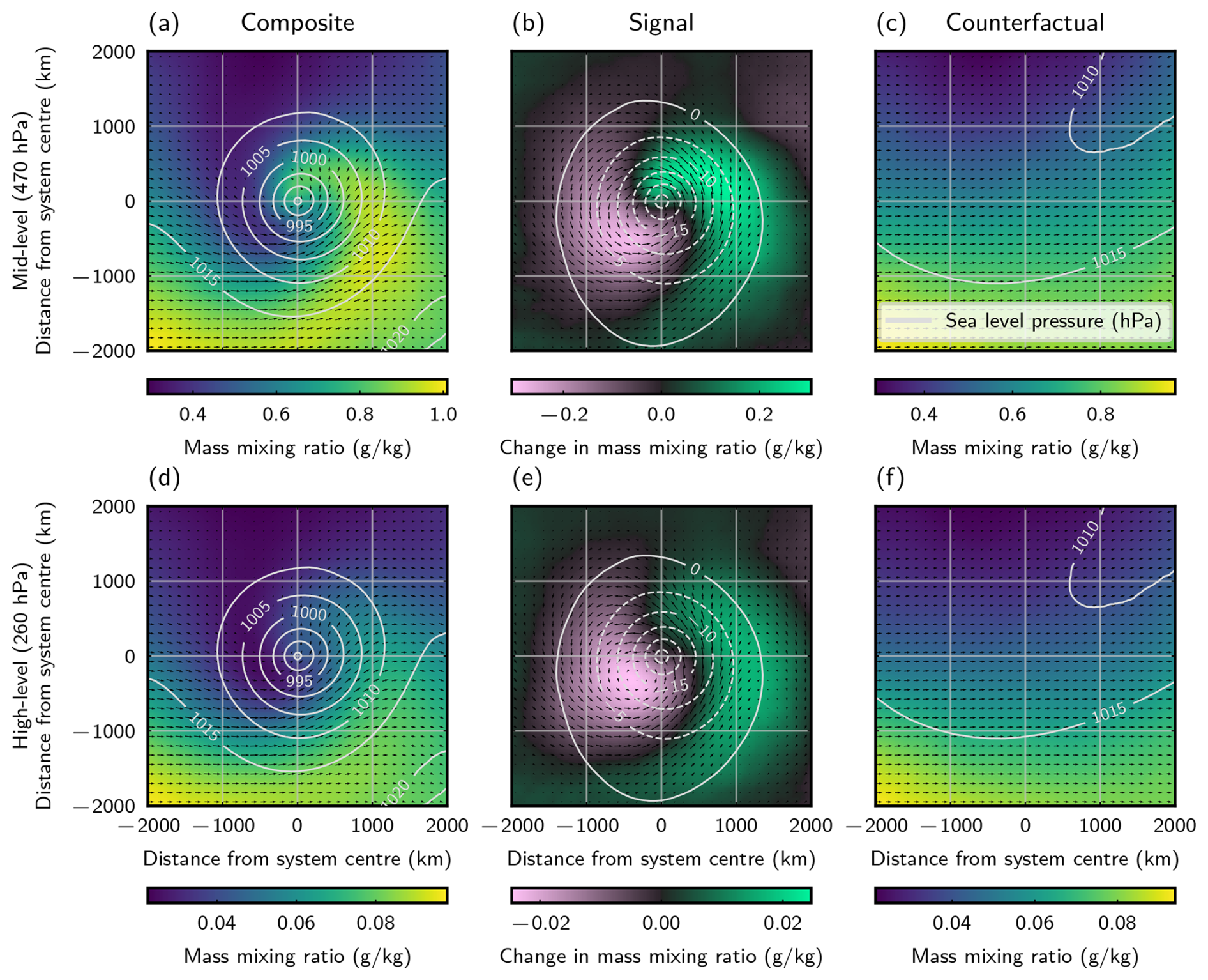
The structure in humidity that is induced by low pressure systems is presented in the body of the manuscript using ISSRs (Fig. 3). While ISSR occurrence is the natural quantity with which to explore the consequences for contrail science, ice processes are less relevant at lower levels, including the “mid-level”, around 470 hPa, as is occasionally examined in this work. Indeed, temperatures at this altitude are often too high for homogeneous freezing of water droplets, or for the Schmidt–Appleman contrail formation criteria (Schumann, 1996) to be met.

In Fig. A1, we present the structure induced in the water vapour mixing ratio. This quantity is conserved within an air parcel, aside from any condensation or evaporation. It exhibits similar structure to that of Fig. 3, though the latitudinal dependence is different. The differences between this and the ISSR composites occur because of structure in temperature, which in turn affects the relevant saturation vapour pressure of ice.

Figure A1 Composite, signal, and counterfactual (as Fig. 3) of the ERA5 water vapour mixing ratio. Data is shown for the two vertical levels presented in Figs 1 and 3.

Appendix B: Composites of relative vorticity

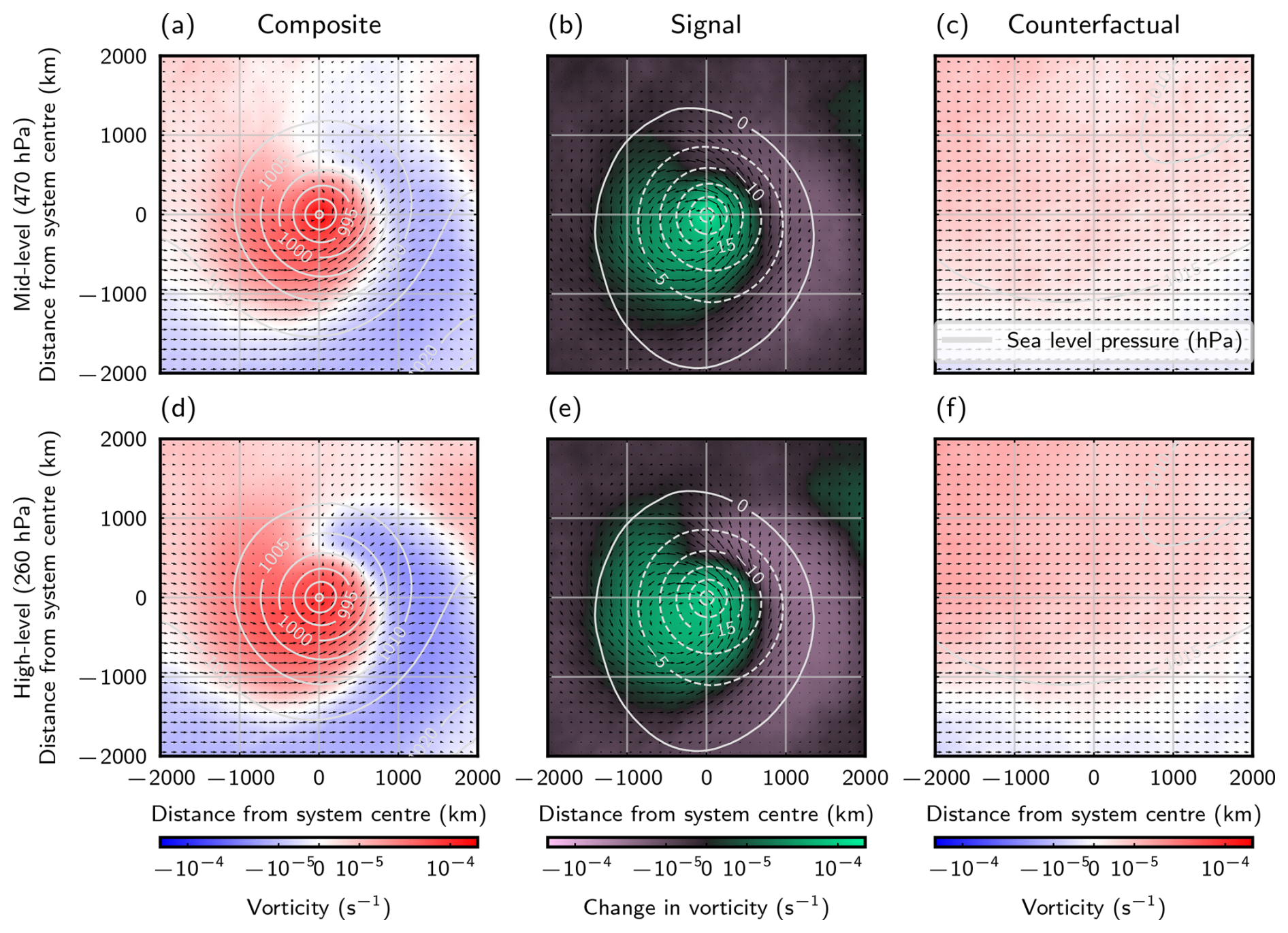
The direction of composited winds (overlaid on Figs. 3–7) can give the impression that the wind around these systems is largely cyclonic, including in the regions of enhanced upper level humidity. This would conflict with the interpretation that these ISSRs occur in the outflow from the warm conveyor belt, where winds tend to turn anticyclonically. This is not the case, as is demonstrated by Fig. B1, wherein the vertical component of relative vorticity (i.e. based on horizontal variations of the horizontal ERA5 winds) is composited. The same sweeping region associated with enhanced ISSR occurrence rate is associated with negative relative vorticity (so anticyclonic winds).

This sweeping region is a result of the trade-offs accepted in order to include as much data as possible (outlined in Sect. 3.1). Therefore, it is important that these composites are not interpreted as a hypothetical state of the weather, but as a lens through which to understand the structure of these systems.

Figure B1 Composite, signal, and counterfactual (as Fig. 3) of the relative vorticity. Data is shown for the two vertical levels presented in Figs 1 and 3.

Appendix C: Composites of flight distance by longitude

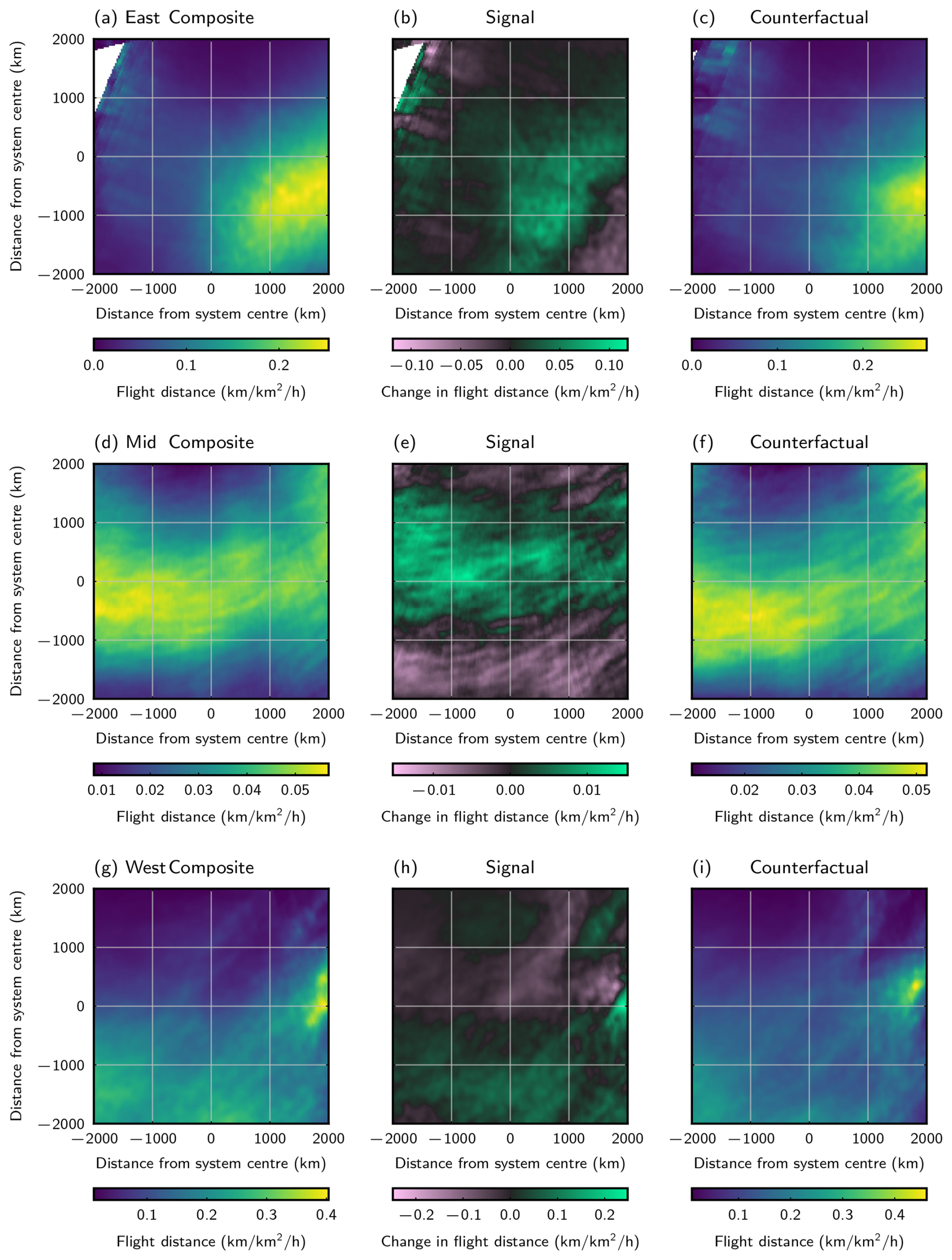
The composite structure of flight distance drawn out by the composites in the body of the article (Fig. 4) shows peaks in air traffic on the east and west edge of composites. This is inferred to be structure resulting from the distribution of routes, specifically, air traffic associated with termini in Europe and North America. In order to break down this signal, composites have been produced of the density of air traffic, and the structure around the low for three longitudinal bands: east of 30° W, between 65 and 30° W, and west of 65° W. This draws out a different set of behaviours. Corresponding composites are shown in Fig. C1.

European air traffic is concentrated south east of the location of low pressure systems; around half of it redistributes closer to the lows in order to take advantage of winds assisting eastbound motion. Over the North Atlantic, air traffic is generally seen to concentrate more in the west than the east, consistent with the behaviour of air traffic, which approaches a more diverse range of latitudes in Europe than when approaching North America; redistribution here is weak compared to the typical air traffic density, but there is a preference for travelling near the lows (where perhaps routes with constructive winds can be chosen). Finally, in the western band, the structure is less clear. A strong peak occurs on the eastern edge of the composite (where a limited number of systems will contribute to the signal); there seems to be a slight preference to fly further south, clear of any disruption from the presence of a low pressure system.

Figure C1 Composite, signal, and counterfactual (as Fig. 3) of flight distance, as in Fig. 4, filtered to only show flights occurring east of 30° W (a–c), between 65 and 30° W (d–f), and west of 65° W (g–i).

Appendix D: The significance of composite signals

In the article, we produce low-centred composites, and counterfactual data sharing the geography and seasonality of lows, which are agnostic to the presence of low pressure systems. Then, we present and interpret the difference between these two composites as a “signal due to the presence of the low”. The structures observed within these signal plots, which extend across regions, are inherently evidence that the comparison, and interpreted signal, is meaningful.

Nonetheless, the opportunity exists to test the statistical significance of difference between the distributions of composited values at corresponding points in the “composite” and “counterfactual” populations. We perform Mann–Whitney U tests (Mann and Whitney, 1947) at each location in the signal, testing the difference between the composite and counterfactual distribution at the 5 % significance level – extended regions of significance reflect independently-validated significance over the structure and therefore provide particularly strong evidence in support of differences due to the presence of the low. Regions of significance are presented for all the signals presented in the body of the article in Fig. D1. All the structures interpreted in this analysis are found to be significant.

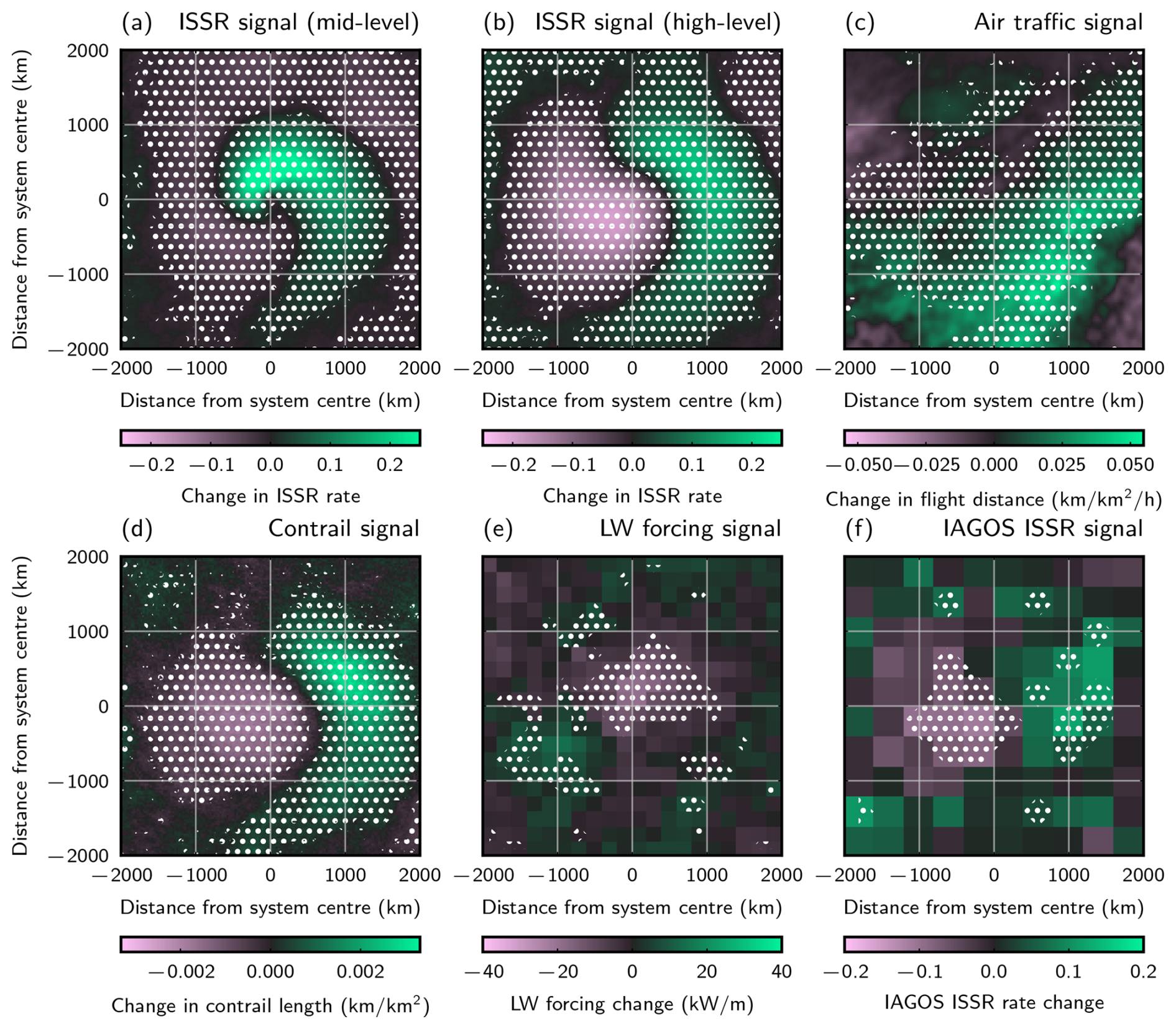
Figure D1 Signal plots as presented in the body of the manuscript, overlaid with dots in regions where the difference between distribution of data in low-centred and counterfactual composites are significant.