Increased dynamic efficiency in mesoscale organized trade wind cumulus clouds

Mesoscale organization of boundary layer clouds modulates their radiative properties and contributes to the tropical hydrologic cycle. Trade wind cumuli (Cu) have varying organization and are a source of uncertainty in global climate models (GCMs). The linkage between Cu development and dynamics is difficult to capture, impacting low cloud feedback estimates. We investigate the relationship between mesoscale organization and Cu updraft dynamics in their early development stages using wintertime shipborne observations. We contrast two periods with similar cloud sizes but more (MO) and less (LO) organized states. MO clouds are dynamically more efficient than LO clouds: for a given core size, MO clouds have stronger sub-cloud and cloud-base updrafts, implying greater vertical moisture transport. Despite similar background plume behaviors, cloud-topped plumes are wider and more frequently successful for MO than LO. Updraft strength is persistent despite diurnal environmental variations. MO turbulence is enhanced by early-morning surface flux maximization and LO updrafts may be assisted by daytime environmental conditions. MO cloud amount persists, while LO clouds suffer daytime depredations. We hypothesize that, once established, MO clouds are maintained through the assistance of cloud-layer-driven mesoscale circulations that increase dynamic efficiency through reinforcing plumes and their updrafts. Dynamic efficiency is likely a key contributor to the moisture–convection feedback critical to mesoscale organization. Organizational modulation of cloud dynamics through enhancing updrafts is another unresolved factor in GCM parameterizations. Understanding this efficiency, and the potential environmental resilience of MO clouds, will be informative for simulating Cu behaviors under current and future climates.

1 Introduction

Clouds occurring over the ocean in the planetary boundary layer (BL, up to ∼ 3 km in altitude) are key components of the climate system. They are important reflectors of sunlight back to space, acting to cool the planet, and can contribute to regional hydroclimate through persistent drizzle, modifying the moisture budget (Hartmann and Short, 1980; Wood, 2012). Marine BL clouds organize into mesoscale patterns (O(100 km)) of clustered cloud structures that vary across the globe (Atkinson and Zhang, 1996; Wood, 2012). This occurs through a process of mesoscale circulations, reinforcing cloud development and persistence, converging moisture into the ascending cloudy branches, and drying the subsiding branches (Bretherton and Blossey, 2017; Narenpitak et al., 2021; Janssens et al., 2023; George et al., 2023). This mesoscale moisture–convection feedback is reinforced through longwave cloud-top cooling in subtropical stratocumulus (Sc) clouds (Bretherton and Blossey, 2017; Zhou et al., 2018; Zhou and Bretherton, 2019b, a) and assisted by gravity waves in tropical trade wind cumulus (Cu) (Bretherton and Blossey, 2017; Janssens et al., 2024, 2023).

Globally, mesoscale organization modulates the radiative properties of BL clouds by separately changing both the amount and optical thickness of cloud (McCoy et al., 2023; Eastman et al., 2024). As clouds evolve from subtropical Sc decks to the west of continents toward the tropics, they transition from more (Sc) to less (Cu) organized clouds (e.g., Eastman et al., 2021, 2022; Sandu and Stevens, 2011; Bretherton et al., 2019; Muhlbauer et al., 2014). Across this transition, the opacity of clouds decreases with an increase in the generation of precipitation-driven, optically thin cloud features at the trade wind inversion (O et al., 2018b, a; Wood et al., 2018; McCoy et al., 2023; Eastman et al., 2024). Once in the tropical trade wind region, cloud amount becomes the key factor in controlling low cloud radiative effects (Bony et al., 2020). Effectively, this is a shift from a cloud widening (Sc) to a cloud deepening (Cu) regime (Feingold et al., 2017), altering the fundamental relationship between cloud brightness and amount (Feingold et al., 2017; Bender et al., 2017). This relationship is something that general circulation models (GCMs), used for climate projections, fundamentally struggle to reproduce (e.g., Engstrom et al., 2015; Bender et al., 2017; Konsta et al., 2022).

The tropical cloud amount–brightness relationship is likely shaped by the moisture–convection feedback reinforcing mesoscale circulations: deepening and brightening Cu in the ascending, aggregating branches while reducing cloud in the descending, drying branches. More clustered Cu cloud are observed to be optically thicker (Alinaghi et al., 2024), have fewer optically thin cloud features (Eastman et al., 2024), and, when normalized by cloud amount, have larger radiative effects (Alinaghi et al., 2024). Mesoscale organization increases both cloud amount (Bony et al., 2020) and opacity in the trades (Alinaghi et al., 2024), increasing the net cloud radiative effect. However, a recent modeling study finds that the net influence of organization on the total radiation budget is small (−0.5 W m⁻²) and persistent even as organization strengthens (Janssens et al., 2025). An ensemble of idealized large eddy simulations (LESs) shows that the constant influence across organization states is due to offsetting effects both across circulation branches and between longwave (LW) and shortwave (SW) effects. As moisture is converged into the ascending branch, clouds are aggregated, reducing cloud amount (SW warming) and deepening Cu (SW cooling) to produce a net SW warming. Simultaneously, descending branches dry the atmosphere (LW cooling). As organization strengthens (e.g., Fig. 1, McCoy, 2025), Cu aggregates and deepens more (enhancing SW warming) and precipitation begins, drying and warming the cloud layers (enhancing LW cooling). This “symmetrical” strengthening of SW and LW effects through mesoscale self-organization maintains the net radiative effect and may be a smaller contribution than the radiative variation driven by the influence of environmental controlling factors on Cu (Janssens et al., 2025).

The sensitivity of low clouds to environmental controls has important implications for cloud response under climate change, a topic of great concern, as well as constraining the representations of low clouds and their feedback in GCMs (e.g., Sherwood et al., 2020; Zelinka et al., 2020; Myers et al., 2021). Subtropical Sc clouds have a substantial positive shortwave feedback on the climate, while the trades have a much smaller, near-zero but still positive feedback, ultimately amplifying the warming from increased concentrations of well-mixed greenhouse gases (GHGs) (Myers et al., 2021; Scott et al., 2020). Mesoscale organization may modulate this shortwave cloud feedback through regional shifts in morphology occurrence frequency driven by environmental changes, influencing cloud optical thickness (and likely amount) in the process (McCoy et al., 2023). This shift in occurrence frequency has already been seen since 1971 in the low-cloud-dominated trade wind dry season (Eastman et al., 2025). Under increased stability, due to uneven warming across the atmospheric column, surface observers have seen an increase in low cloud amount and precipitation, which indicates a climatological shift toward more Sc-like clouds with more optically thin features. This implies a potential negative feedback associated with morphology that may suppress warming and drying in the Caribbean under future climate change (Eastman et al., 2025). Recent work has also found enhanced trade Cu cloudiness over positive sea surface temperature anomalies on the submesoscale to mesoscale as a result of convective updrafts driven by increased surface fluxes (Chen et al., 2023, 2025). Idealized LESs projecting two specific Cu types into the future suggest that mesoscale circulations themselves may be hindered due to increased GHGs, further complicating this issue (Kazil et al., 2024).

GCMs project a much larger, positive feedback in the tropics than observations suggest (Myers et al., 2021; Vogel et al., 2022), overemphasizing trade Cu's response to environmental changes (Nuijens et al., 2015b, a). One explanation for this is overdrying of the BL and cloud base (CB) because of increased lower-tropospheric mixing, entrainment, and large-scale circulations in a warmer world (Sherwood et al., 2014; Zhao, 2014; Brient et al., 2016). Observational and LES studies indicate that trade Cu clouds are actually more resistant to environmental changes (Bretherton et al., 2013; Blossey et al., 2013; Vogel et al., 2016; Nuijens et al., 2014, 2015b). In particular, cloud at CB (i.e., near the lifting condensation level, LCL) is relatively invariant in the trades and controls the overall low cloud amount (Nuijens et al., 2014, 2015b, a). The “cumulus-valve” mechanism (Neggers et al., 2006) has been used as a conceptual framework to help explain the apparent resistance of CB cloudiness to environmental changes: CB amount is proportional to the mass flux through CB (i.e., the updraft velocity scaled by cloud amount and, often, air density). CB mass flux can be thought of as the mechanism through which the moisture–convection feedback operates: lofting moisture into cloud, increasing condensation, and reinforcing the mesoscale circulations. GCMs tend to emphasize thermodynamics (i.e., relative humidity, Quaas, 2012) more than dynamics (i.e., CB mass flux) in their trade Cu dependencies (Vogel et al., 2022). Cu feedback is understandably difficult to simulate as it is a multi-scale problem: their cloud radiative effect is primarily dependent on cloud amount (Bony et al., 2020) but it is being reinforced by mesoscale circulations (Narenpitak et al., 2021; Janssens et al., 2023; George et al., 2023; Janssens et al., 2024) that are not represented in GCMs. Indeed, GCMs poorly capture differences between trade Cu organization regimes in both their absolute behavior and diurnal evolution (Vial et al., 2023). This likely impacts their ability to capture an accurate trade Cu feedback and contributes to uncertainties in climate sensitivity.

The cumulus-valve theory has provided leverage for investigating this multi-scale problem, often by focusing on the relationship between CB amount and mass flux. Progress has been made by observationally constraining this relationship (Vogel et al., 2020; Klingebiel et al., 2021; George et al., 2021; Vogel et al., 2022; George et al., 2023), by investigating how well GCMs capture it (Vogel et al., 2022), and by evaluating its response to future environmental conditions (Vogel et al., 2022; Kazil et al., 2024). Typically in these evaluations, the variability in mass flux is dominated by the variability in cloud amount (e.g., Vogel et al., 2020; Klingebiel et al., 2021; George et al., 2021; Vogel et al., 2022). However, a recent LES ensemble of trade wind Cu indicates that this simple dependence begins to break down as mesoscale structures become larger under greater mesoscale vertical ascent: the contribution to CB mass flux from CB velocity variability becomes more consequential at larger scales although amount still dominates (Janssens et al., 2024). This implies that clouds of different organizational states may have different degrees of mass, and thus moisture, transported into their cloud layers due to the differences in updraft velocity, affecting how moist the BL can become (which has broader implications for the hydrologic budget, see below) and the longevity of clouds (e.g., the persistence of their radiative effects and lack of sensitivity to environmental changes). Mesoscale organization influence on cloud dynamics through increased velocity variability is likely another unresolved factor in GCM parameterizations that is worth considering.

Finally, organized shallow trade wind clouds influence the hydrologic budget of the tropics by playing a critical role in the energetic discharge–recharge cycles that facilitate deep convective precipitation (Wolding et al., 2024). Tropical clouds undergo a shallow discharge–recharge cycle that builds up both heat in the ocean and moisture in the BL, deepening convection toward the free troposphere (FT). Specifically, as trade Cu clouds organize into wider, more Sc-like clusters, convection and moisture deepen in the BL and extend to the FT (Wolding et al., 2024). This is consistent with the moisture convergence and cloud enhancement that occur in the ascending branches of mesoscale circulations through the moisture–convection feedback (Janssens et al., 2024; Narenpitak et al., 2021; Bretherton and Blossey, 2017; Zhou and Bretherton, 2019a). Simultaneously, ocean heat content slowly builds, despite the rapid surface heat flux conversions to atmospheric moist static energy (Wolding et al., 2024). Under the right conditions, the combined BL moistening and deepening of shallow convection (e.g., moisture–convection feedback) and enhancement of ocean heat content and surface fluxes (e.g., surface forcing) leads to a self-amplification of shallow convection (Wolding et al., 2024; Janssens et al., 2024). This enables a transition from shallow to deep convection and the start of a new, deep phase of the discharge–recharge cycle, leading to extensive precipitation through mesoscale convective systems (Wolding et al., 2024).

The potential key role of the moisture–convection feedback, and thus mesoscale organization, in controlling Cu impact on the radiative and hydrologic budget of the tropics motivates two questions: (i) how does the moisture–convection feedback alter Cu updraft dynamics? (ii) At what organization state does this influence begin to appear? To answer these, our study focuses on observationally examining the dynamical differences between organization states of wintertime trade Cu cloud systems as they initially develop. Understanding the early-stage formation dynamics of organized systems allows us to evaluate whether there is a contribution of velocity variability to CB mass flux in less organized environments that grows with circulation scale growth (i.e., Janssens et al., 2024). Impacts on CB mass flux from updraft dynamics have implications for how much moisture is brought into the cloud layer (i.e., influencing the moisture budget through charge cycles) and how bright these clouds can grow (i.e., influencing the radiative budget through deepening and brightening cloud structures). This also has potential implications for the sensitivity of cloud systems to their environment and whether early onset of organization-driven differences in cloud dynamics helps to sustain organized cloud system formation and duration. While addressing these questions does not directly help improve Cu parameterizations within GCMs, it provides broader context for pinpointing processes important to capture in models (e.g., does mesoscale organization matter for capturing the mean cloud state and their environmental sensitivity?).

We leverage a unique set of shipborne observations from a motion-stabilized Doppler wind lidar sampling small cloud structures with little to no precipitation. Observations are taken upwind (approximately 1 d advection, Fig. A1) of Barbados (a benchmark for evaluating tropical cloud behavior, e.g., Medeiros and Nuijens, 2016). On average, these observations capture the earlier stages of the moisture–convection feedback, as described in the theoretical framework from Janssens et al. (2023). As systems advect toward Barbados, mesoscale organization increases aggregation of clouds into larger structures (Eastman et al., 2024; Schulz et al., 2021; Narenpitak et al., 2021; McCoy, 2025) that have more complex dynamics associated with precipitation development (e.g., cold pools, Alinaghi et al., 2025; Zuidema et al., 2017; Vogel et al., 2021). Focusing on small structures also allows us to isolate the influence of local processes rather than synoptic influences (Aemisegger et al., 2021). Observations and their categorization into organization states are described in Sect. 2. A brief summary of current mesoscale organization theory is presented in Sect. 3.1 to contextualize our results. Organizational differences between updraft dynamics and plume characteristics are shown in Sect. 3.2. Evaluation of the environmental sensitivity of these cloud systems including to the diurnal cycle is presented in Sect. 3.3. Implications of these results are discussed in Sect. 4 before they are summarized in Sect. 5.

2 Methods

2.1 Shipborne observations

We utilize in situ observations gathered during the Atlantic Tradewind Ocean–Atmosphere Mesoscale Interaction Campaign (ATOMIC) (Quinn et al., 2021; NOAA, 2020), which was the United States contribution to the international Elucidating the Role of Clouds Circulation Coupling in Climate Campaign (EUREC⁴A) (Bony et al., 2017; Stevens et al., 2021). The NOAA RV Ronald H. Brown (RHB) sampled between 7 January and 13 February 2020 in a region of the ocean between Barbados (60° W) and 51° W, the location of the Northwest Tropical Atlantic Station (NTAS) mooring (Fig. A1). Local time is approximately UTC−4. Generally, the RHB stayed between 16 and 13° N. We used thermodynamic measurements (Thompson et al., 2021a) made on the RHB to investigate the surface and near-surface conditions, ceilometer measurements (Thompson et al., 2021b) to understand the cloud-base height (CBH) behaviors, as well as aerosol measurements (Quinn and Coffman, 2021) and radiosondes (Stephan et al., 2020, 2021) launched every 3 h to investigate the thermodynamic profiles of the atmosphere.

Primarily, we utilized the vertical velocity measurements (Brewer, 2021) captured by the motion-stabilized Doppler wind lidar from NOAA's Chemical Sciences Laboratory (more instrument details in Schroeder et al., 2020; Quinn et al., 2021, 2022). Measurement processing followed the methodology of Lareau et al. (2018), as described in further detail below. Vertical velocity profile measurements were gathered at a rate of 2 Hz and with a vertical resolution of 33.6 m. Once every hour, the lidar performed a conical ∼ 2 min scan at 15° from zenith to retrieve horizontal wind information before returning to its motion-stabilized vertical position. Lidar vertical pointing is stabilized within 0.03° (1σ standard deviation) of zenith, enabling accurate measurements of vertical velocity. Our analysis was focused on the profiles of vertical velocity (w) up to CB, a region that was reliably and consistently observed across the campaign. The lidar signal-to-noise ratio becomes too low above this height due to attenuation by clouds or, when clouds are not present, lack of aerosol above the boundary layer.

For a given Doppler lidar profile measurement, cloud occurrence was identified as where the range-corrected intensity (RCI) of a given pixel exceeded a threshold developed following the method outlined for Cu clouds in Lareau et al. (2018). The RCI threshold was sensitivity-tested and the RCI behavior was compared to the bimodal distribution used to distinguish cloud and aerosol samples in Lareau et al. (2018). The cloud-identified pixels (∼ 0.5 s by 30 m) that occurred lowest in altitude are taken as the CBH. Successive profile measurements where cloud-identified pixels occurred within 10 s and 50 m of each other were aggregated together into a single cloud scene. The reference CBH of the cloud scene is calculated as the 25th percentile of CBH across the aggregated profiles composing the total scene (Lareau et al., 2018). This method produced a Doppler lidar CBH that agreed well with the ceilometer observations (Fig. 11a, Quinn et al., 2021). The length of a cloud is defined as the duration of the cloud scene scaled by the horizontal wind speed at CB, which is interpolated from the hourly horizontal velocity measurements from the lidar (chord length, L_Chord). Because we were interested in the behavior of developing or active clouds, we further restricted our dataset to cloud scenes with a CBH within 50 m of the LCL. The LCL was determined from an adiabatic parcel model initialized with thermodynamic observations from the RHB.

Each cloud scene can be thought of as a snapshot of vertical velocity behaviors occurring around a single cloud. Cloud scenes were processed into normalized w matrixes for ease of computations (Lareau et al., 2018), where length is normalized by total cloud length at CB (−1.5 to 1.5 in $x/L_{\mathrm{Chord}}$ where cloud occurs between −0.5 and 0.5) and altitude is normalized by CBH (0 to 2 in $z/\text{CBH}$ where CB is at 1). Figure 1a shows an example normalized w matrix for a cloud scene, highlighting a plume connecting from the surface to CB and observable partway into the cloud before attenuation. The sub-cloud and CB updraft region where our analysis is focused is marked: −0.5 to 0.5 in $x/L_{\mathrm{Chord}}$ and 0 to 1 in $z/\text{CBH}$.

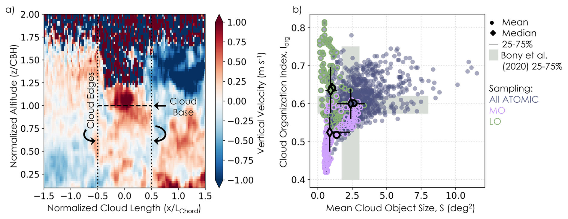
Figure 1 (a) Individual cloud vertical velocity measurement example shown in normalized altitude (by cloud-base height) and cloud length (by chord length) space. Cloud edges and base are marked for reference. (b) Campaign days (dark purple) in I_org vs. S space with MO (purple) and LO (green) highlighted. Mean (circle), median (diamond), and 25 %–75 % (lines) for the MO, LO, and total campaign data composites are included. Gray shading in the background shows the interquartiles ranges used to define the SGFF quadrants in Bony et al. (2020) for reference, as in Schulz (2022a).

The CB amounts from the individual Doppler lidar cloud scenes and the ceilometer have statistically similar magnitude and broadly similar diurnal cycle shapes (Fig. A4a, c). Ceilometer CB amount was derived from the 15 s data product for first cloud-base detection restricted to CBH ≤ 800 m (the upper quartile of MO CBH, Fig. 12b). This is a different sampling rate than the Doppler lidar (which excludes clouds smaller than 10 s in duration) and an approximate CBH cut-off picked to correspond to the more exact LCL restriction applied to the Doppler lidar scenes. These retrieval and resolution differences likely contribute to the differences in cycle details. However, the general statistical agreement and similarity in cycle shape indicate that the sampling of the identified cloud scenes is comprehensive for this period of low, active clouds.

We were additionally interested in the behaviors of thermal plumes sampled by the lidar. A plume is defined as a contiguous region where w > 0.05 m s⁻¹. The plume horizontal length (L_Plume) is taken as the maximum diameter of the plume measured in seconds and converted to meters using the interpolated, hourly surface wind speed where the surface is ∼ 60 m, the lowest measured altitude for the Doppler horizontal wind. Because not all plumes are topped by clouds and have varied depth, we utilized the surface wind to be consistent across all plume features. However, the wind shear between this altitude and the CB is negligible so the length conversions are comparable across cloud and plume features with little bias (Fig. 9). Note that this analysis is agnostic to the number of plumes contributing to the maximum plume length as, due to the nature of the cross-sectional sampling of the lidar, we are not able to robustly distinguish between multiple overlapping plumes and one wide plume contributing to the contiguous plume feature. Plumes are labeled as cloud-topped if the plumes occur within 1 min of a cloud identification that has a positive updraft at CB (L_{Plume Cloud}). Otherwise, they are assigned to be clear-sky (i.e., “unsuccessful” plumes, L_{Plume Clear}).

We further restricted the cloud identification data to examine clouds with active CB cores (w_CB > 0). We defined the CB core updraft for individual clouds (w_CB Core) as the mean of CB values that satisfied w_CB > 0. The corresponding CB core length (L_CB Core) for individual clouds is defined as the total cloud length, L_Chord, scaled by the fraction of the samples that contribute to the active CB core. In the example w matrix in Fig. 1a, the plume noticeably strengthens near CB and in cloud, marking the core updraft. In addition to the CB core observations, we analyzed sub-cloud updraft profiles (w >0). We do not include the samples outside of cloud (i.e., < −0.5 and > 0.5 in x, Fig. 1a) as they may be contaminated by nearby clouds. For this reason we also do not analyze downdrafts as they are likely incomplete, falling largely outside of the sub-cloud range.

We are not able to sample in heavily precipitating conditions. This did not pose a significant issue as there were few instances of precipitation (Zuidema, 2021) recorded on the RHB (Quinn et al., 2021). The RHB tended to sample much further upwind compared to the other platforms during EUREC⁴A, observing earlier in the evolution of clouds, before precipitation and the accompanying cold pools developed (Touzé-Peiffer et al., 2022). This suggests that these observations are particularly well suited for investigating the early stages of Cu clouds in this region, adding context to their early behaviors before the clouds reach the main EUREC⁴A domain and Barbados.

2.2 Cloud organization identifications

The goal of our comparison is to contrast organized cloud structures with unorganized ones. Distinguishing by organization was a nontrivial task. Mesoscale structures have been variously categorized in recent years (e.g., Wood and Hartmann, 2006; Rasp et al., 2020; Yuan et al., 2020; McCoy et al., 2023; Janssens et al., 2021; Denby, 2020; Lang et al., 2022; Chatterjee et al., 2024; Warren et al., 2011) to investigate their influence on the climate system. One such methodology (Rasp et al., 2020) developed a neural network to categorize four archetypal cloud types based on expert assessments (SGFF: sugar, gravel, flowers, and fish) to aid trade Cu investigations (e.g., Stevens et al., 2019; Bony et al., 2020; Schulz et al., 2021; Vial et al., 2021). This algorithm, along with hand identifications from the EUREC⁴A team, were applied to GOES-16 and MODIS satellite scenes over the EUREC⁴A region and campaign period to develop the C³ONTEXT dataset (Schulz, 2022a, b). Our initial analysis utilized C³ONTEXT SGFF identifications collocated to the location and time of RHB sampling (see Hovmüller diagram, Fig. A1). However, many cloud samples could not be confidently labeled as one of the SGFF types, leading to a large number of unclassified (Schulz, 2022a) or “none” types dominating the sampling (Fig. A1). This presented a problem for analyzing the comparatively sparse campaign sampling, unlike analyses based on multiyear satellite climatologies (e.g., Bony et al., 2020; Schulz et al., 2021; Vial et al., 2021).

To maximize the number of cloud scene identifications utilized, ensuring more reliable statistical sampling, we developed a more general classification methodology: hand-identifying clouds into two categories, less (LO) and more (MO) organized structures. We relied on MODIS Aqua (13:30 local time, LT) and Terra (10:30 LT) satellite imagery to identify the daily cloud field where the RHB was sampling (see imagery used for classification in Figs. A2 and A3). The LO category (Fig. A2) comprised days where only small, scattered structures occurred randomly (30 and 31 January and 1, 4, and 9 February; 1356 lidar cloud scene identifications, 1275 cloud-topped plumes, and 27 040 clear-sky plumes). The MO category (Fig. A3) comprised days where more discernibly clustered structures as well as some smaller structures occurred in larger patterns of organization (9, 10, 11, 12 January and 10 and 11 February; a total of 2539 cloud scenes, 2492 cloud-topped plumes, and 29 284 clear-sky plumes). LO days included sugar-dominated cloud scenes and MO included gravel and a few flowers-like cloud scenes.

The LO and MO categorized days, which will be used for compositing throughout the rest of the paper, help us to distinguish between cloud systems that have not been substantially influenced by mesoscale organization and are still occurring fairly randomly (LO, Fig. 2a) and those that have already been influenced enough by mesoscale circulations generated through the moisture–convection feedback to begin gathering into discernible mesoscale organization patterns (MO, Fig. 2b). Different LO and MO sample sizes are accounted for by utilizing standard error to determine confidence in the mean and statistical tests for determining distribution differences at 95 % confidence. Days where very large cloud structures associated with the decay of midlatitude cold frontal cloud systems (i.e., fish, Schulz et al., 2021; Aemisegger et al., 2021) were not included in our analysis to focus on locally driven cloud systems, as previously noted. We extract the full diurnal cycle based on the daytime cloud identifications to obtain a cohesive signal that can be compared to the corresponding environmental cycles without adding additional complexity in interpretation from day-to-day variations. Although organization varies diurnally (Narenpitak et al., 2023, 2021; Koren et al., 2024; Denby, 2023), it would be challenging with our small sample size to ensure a complete cycle was captured and appropriately connected to environmental behaviors if classifications were made at a greater temporal frequency (e.g., Vial et al., 2021; Schulz et al., 2021, where the larger sample size eases these concerns).

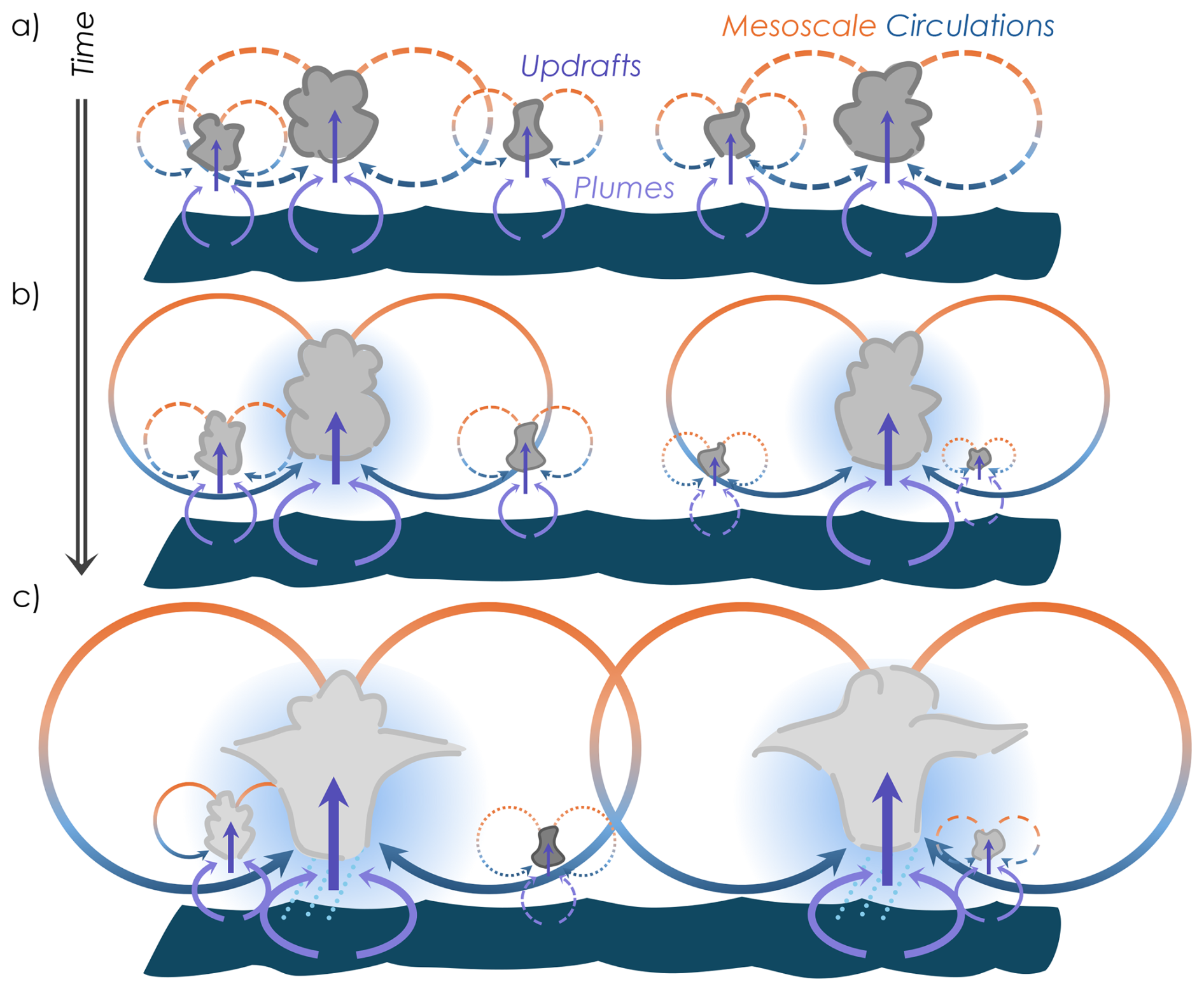
Figure 2 Evolution of trade Cu clouds as they organize with time (a–c) through strengthening of mesoscale circulations (orange to blue arrows) via moisture–convection feedback (see Sect. 3.1). Dynamic efficiency is represented through strengthening of updrafts (vertical arrows) as organization intensifies, accompanied by wider plumes (purple curved arrows), more moisture aggregation (blue haze), and greater plume success rates in ascending branches (new cloud starting at right, b–c).

To confirm that this coarse LO–MO separation distinguished measurements by organization as intended, we additionally compared these categorizations with two objective classifiers also included in the C³ONTEXT dataset: the mean cloud object size (S) and the organization index (I_org, which compares the distribution of nearest-neighbor distances between centroids to a random distribution) (Schulz, 2022a). This phase space has been reliably utilized to classify trade Cu (e.g., Bony et al., 2020; Schulz, 2022a; Janssens et al., 2021). I_org and S were calculated on 10 × 10° brightness-temperature-defined scenes of cloud amount (as in Bony et al., 2020), approximately centered on the EUREC⁴A region. They were then collocated to the location and time of the RHB sampling (Fig. 1b). Note that this comparison is approximate since the RHB was often sampling on the edge of this domain, not at its center. The interquartile ranges corresponding to the SGFF archetypes in Bony et al. (2020) are shown for reference following Schulz (2022a). The LO data tend to fall in the sugar quadrant (lower S, higher I_org), while the MO data tend to fall in the gravel quadrant (lower S, lower I_org). The apparent greater organization of LO (I_org > 0.5) follows the behavior of sugar discussed in Bony et al. (2020). This counterintuitive behavior is likely a feature of the brightness temperature thresholds, which are more sensitive to the sparsely distributed deeper clouds in these scenes than the dominate low clouds. Overall, this comparison indicates that (i) the visual categorization described above successfully separates observations by organization to the first order (y axis) and (ii) both LO and MO will span similar cloud structure sizes (x axis). This is fortuitous as it allows us to focus on organization without the additional complexity of structure size contributing to cloud behavioral differences (i.e., as would occur at later stages of organization development when precipitation and cold pools begin to play a role, Fig. 2c).

3 Results

3.1 Mesoscale organization theory

Our results will be presented in the context of the current theory on how mesoscale organization influences Cu in the tropical trade winds (e.g., Bretherton and Blossey, 2017; Narenpitak et al., 2021; Janssens et al., 2023, 2024; George et al., 2023), as summarized in Fig. 2. Cu clouds develop randomly when surface-driven, thermal plumes (purple curved arrows) cohere into updrafts (purple vertical arrows) and rise past the LCL, condensing moisture and releasing heat (a, LO). To maintain the tropical weak temperature gradient approximately, gravity waves export heat from the clouds, generating mesoscale circulations (orange to blue arrows). Circulations begin to aggregate moisture in their ascending branches (blue haze, b), gathering more moisture into Cu clouds that can in turn generate more condensational heat and trigger more gravity waves, reinforcing mesoscale circulations and deepening Cu. This moisture–convection feedback transitions non-precipitating cloud fields from LO (a) to MO (b) through generating more organized cloud structures over time. Note that Janssens et al. (2024) find that the growth rate of cloud layer heating and mesoscale velocities cannot be explained by rapid convective adjustment to surface buoyancy flux anomalies, indicating that this organization is likely not driven by mesoscale surface forcing. Clouds in the descending branches will experience more dry, subsiding conditions and begin to die. Eventually, through moisture–convection feedback developing wider (i.e., length-scale growth of moisture fluctuations, Janssens et al., 2023) mesoscale circulations (George et al., 2023), clouds will be organized into larger-scale patterns (e.g., flowers, c) that are deep and bright and begin to precipitate (Narenpitak et al., 2021; Janssens et al., 2024). The cold-pool downdrafts associated with stronger precipitation as these features continue to strengthen will eventually disrupt the updraft reinforcement cycle and break this moisture–convection organization feedback (not shown). Results have been incorporated into Fig. 2 and will be highlighted in Sect. 3.2 and 3.3.

3.2 Dynamic efficiency of organized clouds

The central goal of this work is to identify whether there is a detectable difference in cloud dynamics across mesoscale organizational states in the early stages of cloud development (i.e., LO vs. MO in Fig. 2a, b). The results will inform our understanding of how the moisture–convection feedback affects cloud dynamics as mesoscale organization strengthens. We began by comparing the MO and LO composites of updraft velocity mean (panel a) and variance (panel b) profiles computed for individual cloud scenes (Fig. 3). For each composite, here and throughout the paper, the mean and 95 % confidence in the mean (twice the standard error, 2 SE) are shown for each vertical bin (either in altitude or normalized altitude space, $z/\text{CBH}$, as shown here). We apply the Mann–Whitney U test for each bin to test whether the nonparametric distribution of the MO and LO data is statistically likely to have come from the same population at 95 % confidence.

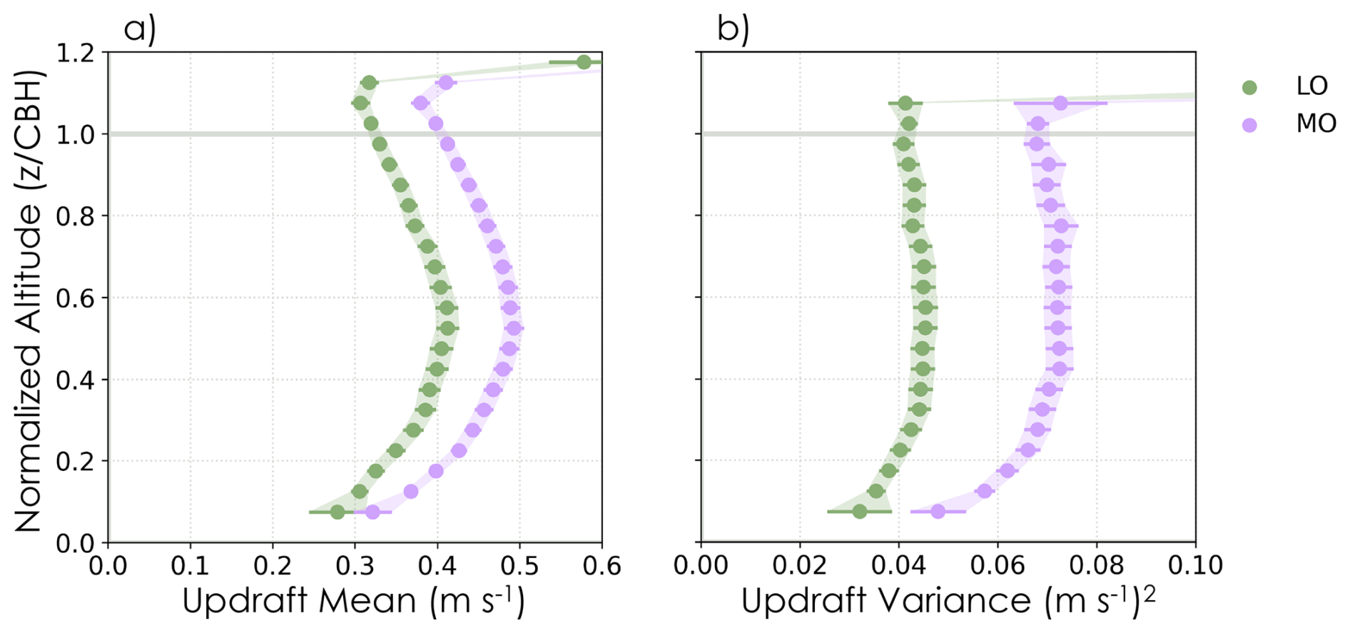
Figure 3 MO (purple) and LO (green) composites of updraft profiles of (a) mean and (b) variance of vertical velocity. Shading and horizontal lines represent 2 SE in the mean (circles) for vertically binned data. Filled circles are where the MO and LO distributions are different at 95 % confidence based on the Mann–Whitney U test.

MO clouds have larger mean updrafts that are from a statistically different population than the LO cloud updrafts throughout the sub-cloud layer, CB, and into the observable lower cloud layer prior to lidar attenuation (Fig. 3a). This organizational difference also holds for the mean variance in the updrafts (Fig. 3b), indicating that MO clouds have greater turbulence than LO on average in addition to having more powerful updrafts.

In Fig. 3, all cloud sizes are included in the organization composites. On average structure sizes are similar between MO and LO (Fig. 1b) but it is worth testing for variations in behavior across cloud size. For example, the mean MO–LO separation could be influenced if there was disparity in updraft region size and the subsequent core area of the cloud. Additionally, if one organization state tended to have larger updraft regions their cores may be more protected, increasing the number of strong updrafts and shifting the mean to larger values compared to the other organization states. To address both of these issues we composited MO and LO clouds by L_CB Core ranges (Fig. 4), which is also generally informative of cloud size separation (e.g., Fig. 6d–e) assuming minimal horizontal expansion and tilting with height (e.g., Fig. 14 for sugar and gravel, Schulz et al., 2021). The selection of L_CB Core ranges is based approximately on the quantiles of the distribution of cores across the data such that similar amounts of low cloud are captured for each core range. In both organization states, a majority of clouds occur in the 0 to 500 m and 500 m to 1 km ranges and progressively fewer occur in the 1 to 2 and 2 to 7 km (Fig. 6e). This indicates that the total mean results (Fig. 3) are weighted toward the smaller clouds, which makes their substantial differences even more notable.

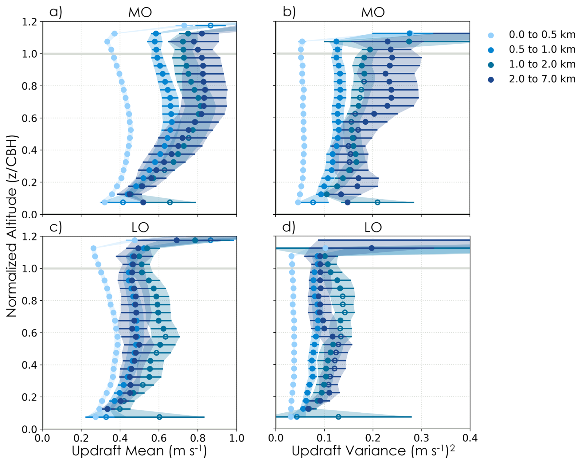
Figure 4 MO (a–b) and LO (c-d) composites of updraft mean (a, c) and variance (b, d) profiles for different cloud core sizes. Shading and horizontal lines represent 2 SE in the mean (circles). Filled circles are where the MO and LO distributions are different at 95 % confidence based on the Mann–Whitney U test for the given L_CB Core range.

The resulting profiles for updraft mean (Fig. 4a, c) and variance (Fig. 4b, d) composited by L_CB Core provide three insights. First, MO updraft mean and variance are larger and significantly different at 95 % than LO updrafts for all L_CB Core ranges across the majority of the cloud and sub-cloud altitudes. The few exceptions to this are likely impacted by sampling as they occur at the surface and in the larger L_CB Core ranges, exhibiting wider 2 SE bars. For the mean updrafts, the 1 to 2 km range has several bins in the lower half of the sub-cloud layer where MO and LO are not statistically different. For the updraft variance, 1 to 2 and 2 to 7 km composites have several bins in the upper and lower half of the sub-cloud layer, respectively, that are not statistically different. This overlap pattern leads to the second insight. With increasing organization, cloud-topped plumes increase in updraft strength but strengthening appears to occur more in the upper sub-cloud layer and CB region. This suggests that the organization-dependent influence on the updrafts is associated with a cloud layer phenomenon. For example, updrafts may be assisted by the returning branches of mesoscale circulations generated by condensational heat release in the cloud layer. This organizational strengthening could play an integral role in the moisture–convection feedback (Fig. 2a, b). Third, with progressively larger L_CB Core ranges, updraft magnitudes increase (Fig. 2b, c). The LO composite is an exception to this, staying relatively consistent across the three largest L_CB Core ranges. This discrepancy in behavior between LO and MO is intriguing, suggesting that LO w_CB Core is less assisted by the cloud layer phenomenon, while MO w_CB Core can continue to strengthen with increasing cloud core size. This may indicate greater differences in cloud layer influence or contributions from environmental factors (see Sect. 3.3).

Similarly, we evaluate the behavior of the updrafts across the diurnal cycle (Fig. 5). For all times of day, MO updraft mean and variance are larger and come from a statistically different population than LO updrafts at 95 % confidence. Within their respective composites, MO and LO updrafts are relatively persistent and do not have statistically robust diurnal cycles in w_CB Core at 95 % confidence. An exception is the distinct peak in w_CB Core variance for MO at the end of the night (06:00–12:00 UTC or 02:00–08:00 LT, b; 10:00 UTC or 06:00 LT, f), recovering from a nighttime lull (05:00 UTC or 01:00 LT, f). Mean MO w_CB Core echoes this lull and recovery (c). LO may experience an increase in mean and variance at the end of the day, peaking enough sub-cloud and at CB (18:00–24:00 UTC, or 14:00–20:00 LT, c, f) to overlap statistically with MO. These deviations from the constant w_CB Core mean and variance suggest that different factors may contribute to MO and LO updrafts over the day: LO appears more tied to the solar influence, while MO may be more influenced by nighttime factors. The order of LO updraft magnitudes also lags between the mid-plume height (0.5 $z/\text{CBH}$, 00:00–06:00 UTC, d) and CB, indicating a potential lag between the surface influences and their impact on clouds. This lag is not apparent for MO, which has similar profile ordering throughout (a, b), suggesting the cloud layer may support the plume strength when surface influences are declining. We will return to this in Sect. 3.3.

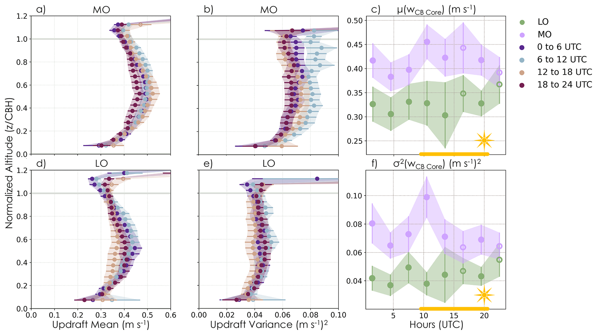
Figure 5 MO (a–b) and LO (d–e) composites of updraft mean (a, d) and variance (b, e) profiles for different times of the day in UTC. The diurnal cycle of CB updraft velocity mean (c) and variance (f) is shown for MO (purple) and LO (green). The local daytime (yellow line, sun) is shown for reference in panels (c) and (f). Shading and horizontal lines represent 2 SE in the mean (circles). Filled circles are where the MO and LO distributions are different at 95 % confidence based on the Mann–Whitney U test.

To gain a more holistic understanding of the updraft differences, we also evaluated the differences in plume and cloud size characteristics across organization states. First, we contrasted the distribution of the plume maximum horizontal lengths in clear-sky (a, “unsuccessful”, L_{Plume Clear}) and cloud-topped (b, “successful”, L_{Plume Cloud}) conditions (Fig. 6). L_Plume exponentially decays with size for all cases, changing in slope around 2 to 3 km. Unsuccessful plumes occur more frequently than successful ones across all lengths and organization states (a vs. b). This is consistent with relatively low CB cloud fractions. Diurnal mean cloud amount is ∼ 9.5 % for LO and ∼ 13 % for MO, with 2 % 2 SE for both (Fig. A4a, c). While the mean CB amounts are statistically similar, the lower L_{Plume Cloud} numbers for LO may be associated with the larger diurnal cycle in LO than MO: LO cloud amount is minimized between 08:00 and 16:00 UTC (04:00 and 00:00 LT), while MO holds steady (Fig. A4).

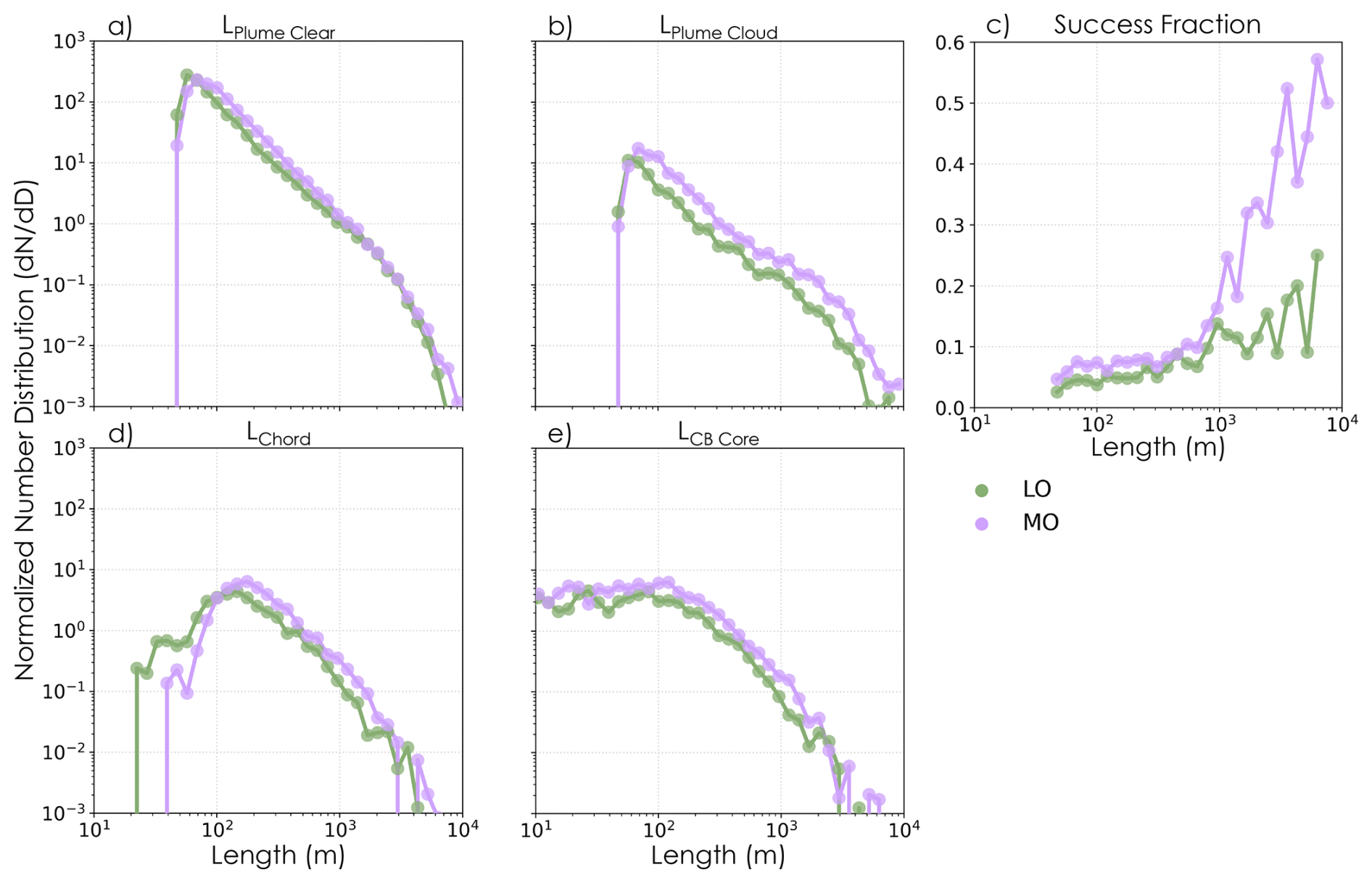
Figure 6 MO (purple) and LO (green) normalized size distributions for clear-sky (a) and cloud-topped (b) plume widths and the cloud chord (d) and core (e) lengths. MO and LO distributions are different at 95 % confidence based on both the Mann–Whitney U test (rejecting the null hypothesis that the underlying distributions are the same) and the Kolmogorov–Smirnov test (rejecting the null hypothesis that the data were drawn from the same distribution). (c) Plume success fraction computed as the ratio of the cloud-topped (b) to clear-sky (a) plume width number distributions.

For a given L_Plume, MO has more successful plumes than LO (Fig. 6a–c). MO plume success appears to increase more with L_{Plume Cloud} than for LO (i.e., the rightward shift of the MO L_{Plume Cloud} distribution and divergence after ∼ 100 m, b). Notably, this organizational difference is not apparent in the unsuccessful, L_{Plume Clear} distributions (a). We compute the plume success fraction (c) as the ratio of number distributions between the L_{Plume Clear} and L_{Plume Cloud} to clarify this tendency. Plume success increases with L_Plume for both organization types, but the MO success rate increases far more rapidly, diverging from LO after 1 km. This organizational difference in success rate is another potential marker of cloud-layer-driven mesoscale circulation, e.g., through the ascending circulation branch cohering plumes into stronger updrafts and lowering the LCL through converging moisture (Fig. 2a, b). For a given plume width, MO clouds likely have deeper (e.g., Fig. 12c) and moister clouds due to the moisture–convection feedback. As plumes increase in size, potentially through turbulent enhancement by mesoscale circulations, they can also support larger clouds. Thus, MO clouds for L_{Plume Cloud} > 1 km have an exponentially greater potential to generate heat through condensation release, which will further reinforce mesoscale circulations, plume success rate, and organization.

Second, we evaluated the total (c, L_Chord) and CB core (d, L_CB Core) lengths and found organizational differences apparent in their distributions as well. Specifically, MO clouds tend to be generally larger than LO clouds but with substantial overlap. MO clouds occur more frequently with larger L_Chord and less frequently with smaller L_Chord than LO (i.e., MO shifted to the right of LO, c). This also holds for L_CB Core with large cores occurring more frequently for MO (d). The CB core cloud amount from L_CB Core (∼ 7 ± 2 % for LO and 8.9 ± 0.6 % for MO, Fig. A4b) is, as expected, smaller than the amount derived from L_Chord, but both CB and CB core amounts are statistically similar between MO and LO on average and both exhibit persistent MO and an apparent solar burn-off/recovery cycle for LO. Note that L_{Plume Cloud} tends to be wider than the cloud and core lengths they support (i.e., L_Chord and L_CB Core distributions are shifted left relative to the plumes, b–d; relationship is not 1:1 in Fig. 7a). Recall that L_{Plume Cloud} pertains to the maximum width of the contiguous region, not the plume core, and likely includes turbulent tendrils.

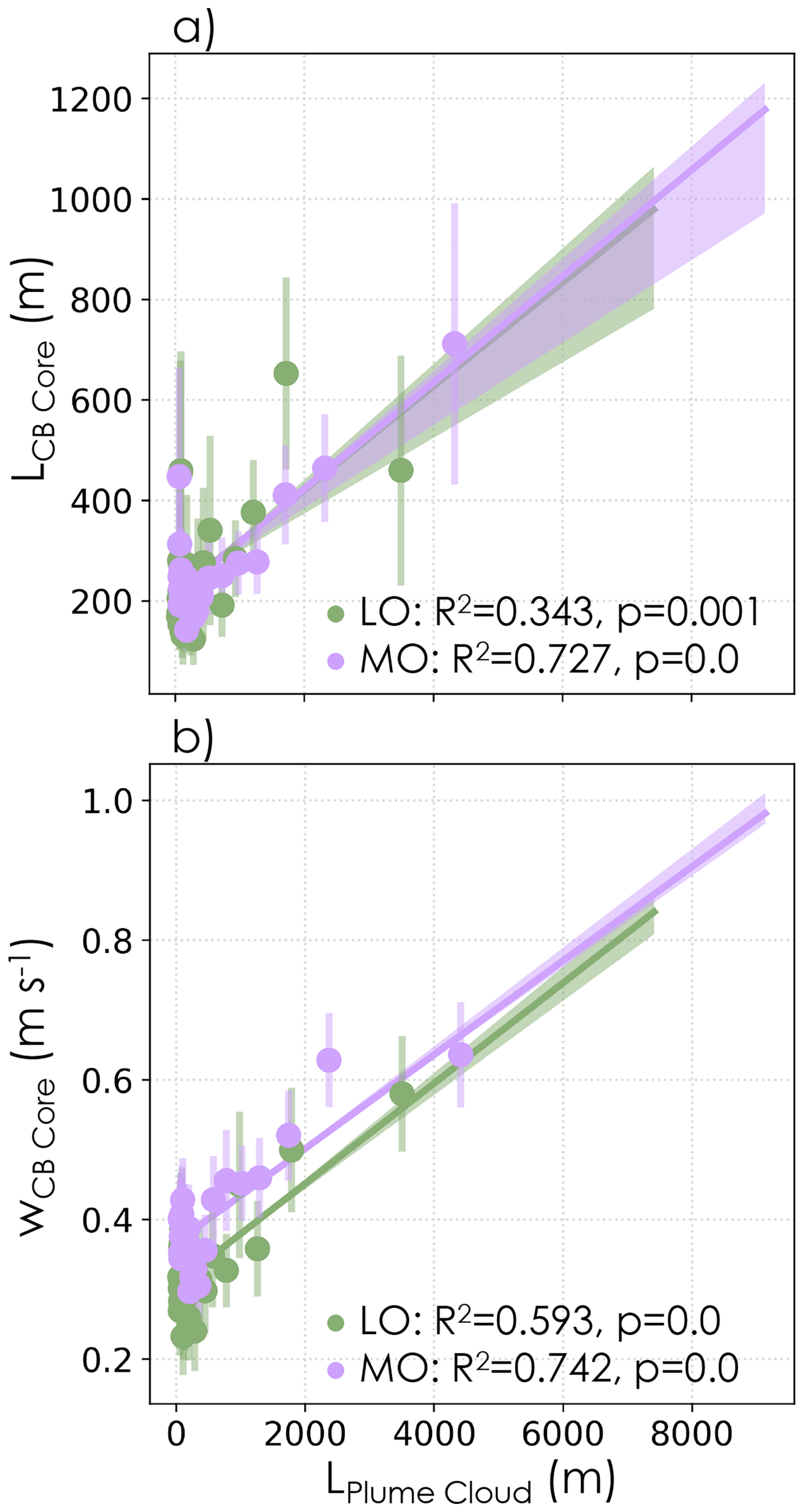
Figure 7 MO (purple) and LO (green) comparisons between cloud-topped plume widths and (a) CB core velocity and (b) lengths. Best-fit linear regressions are computed on the underlying data with confidence intervals (min and max, shading) calculated using the jackknife method (Tukey, 1958). Mean (dot) and 2 SE (vertical shading) for quantiles of plume width illustrate the distribution of data. Correlation coefficients for quantile relationships are significant at 95 % confidence.

The tendency toward larger L_Chord and L_CB Core for MO clouds is consistent with the expectation that they have undergone more organization. Organizational differences manifesting primarily in L_{Plume Cloud} indicate that plumes may be reinforced by a cloud-associated process, potentially including cloud-layer-driven mesoscale circulations (i.e., Fig. 4). The reinforced plumes likely feed back on clouds through supporting stronger cloud updrafts in the ascending branches of mesoscale circulations, increasing cloud success rate and helping to cluster clouds further through the moisture–convection feedback (i.e., by lofting more moisture into cloud, generating more condensation, and strengthening the moisture-converging mesoscale circulations, Fig. 2a, b).

To understand whether the organizational differences in plume behavior impact CB dynamics and thus CB mass flux, we contrasted the relationships between L_{Plume Cloud} with L_CB Core and w_CB Core (Fig. 7). Because of the different plume width distributions between LO and MO (Fig. 6b), the CB core variables have been binned into quantiles by L_{Plume Cloud} for ease of comparison. Linear regressions are performed on the underlying data. Hypothetically, for a given L_{Plume Cloud}, a stronger relationship with MO L_CB Core would indicate that wider plumes support larger core area, e.g., through more cloud aggregation in ascending circulation branches. A stronger relationship with MO w_CB Core would suggest that mesoscale circulations affect the updraft dynamics directly, e.g., contributing dynamically through strengthening the updrafts in ascending branches. Wider plumes associated with more organization could be supporting both of these effects, modifying CB mass flux in two ways.

It is apparent that both LO and MO clouds have statistically indistinct linear relationships between L_{Plume Cloud} and L_CB Core (Fig. 7a; L_Chord has similar behavior, not shown, with R² (p) = 0.594 (0.0) and 0.25 (0.006) for MO and LO, respectively). The increased frequency of larger L_{Plume Cloud} for MO (i.e., wider quantile distribution and Fig. 6b) is consistent with the marginally more frequent occurrence of larger L_CB Core (Fig. 6e). Based on regressions on the quantile binned values, more variance is explained in L_CB Core by L_{Plume Cloud} for MO (73 %) than LO (34 %). While this indicates that plume width more directly translates to core size in MO, the similarity in relationships between LO and MO suggests that core size has not been significantly modified by organization effects (e.g., cloud aggregation) at this stage of cloud development (Fig. 2a, b). More organized stages beyond MO may see a larger impact (Fig. 2c).

The organizational differences are much larger in the relationship between L_{Plume Cloud} and w_CB Core (Fig. 7b). Best-fit linear regressions are statistically distinct between LO and MO for the range encompassed by the majority of the observations (L_{Plume Cloud} through ∼ 6 km). The variance explained in the quantiles is substantial for both MO (74 %) and LO (60 %). The offset between the LO and MO lines is a clear indication that for a given L_{Plume Cloud}, MO clouds have stronger w_CB Core than in LO clouds. These comparisons mark an important finding: for a given plume width, and thus core length, MO clouds achieve stronger CB core velocities and have increased mass flux into the cloud layer. This may be a manifestation of returning cloud-layer-driven mesoscale circulations boosting updraft strength in their ascending branches (Fig. 2a, b).

Finally, we evaluate these organizational differences in cloud behavior using the classic cumulus-valve phase space from the literature (e.g., Klingebiel et al., 2021; Vogel et al., 2022: w_CB Core vs. L_CB Core) (Fig. 8). Because the range of L_CB Core is more similar than L_{Plume Cloud} (Fig. 6b vs. e), we can use the same quantiles for LO and MO L_CB Core and use the Mann–Whitney U test to statistically evaluate distribution overlap in each quantile. This strategy is also advantageous since the L_CB Core vs. w_CB Core relationship is distinctly nonlinear. Note that linear regression fits are statistically well separated for MO and LO (Fig. B1). Regression on LO and MO quantiles indicates that 49 % and 66 %, respectively, of the variance in w_CB Core is explained by L_CB Core (separate LO and MO quantiles have lower correlations of 40 % and 59 %, Figure B1).

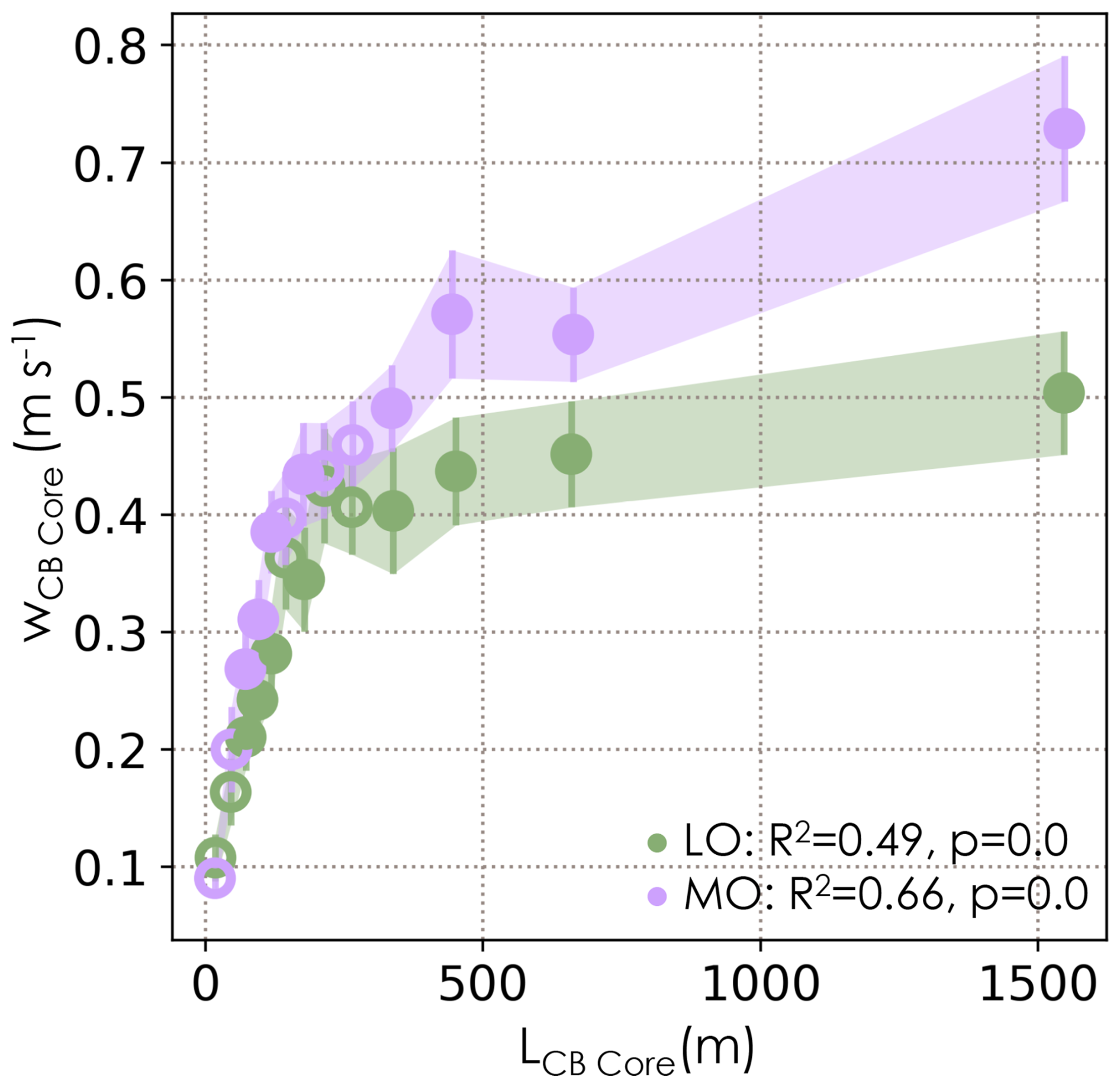
Figure 8 MO (purple) and LO (green) composites of CB core size (L_CB Core) vs. velocity (w_CB Core). The mean (circle) and 2 SE (shading, vertical lines) of w_CB Core are plotted in quantiles of L_CB Core computed from the combination of LO and MO distributions. Filled circles are where the MO and LO distributions are different at 95 % confidence based on the Mann–Whitney U test.

We find, in agreement with prior evaluations (Sect. 1), that stronger w_CB Core is associated with more cloud at CB (i.e., greater L_CB Core). However, there are two important nuances revealed in Fig. 8: (i) MO clouds have consistently larger mean core updrafts (i.e., the MO curve is higher than the LO curve, consistent with Figs. 6e and 7b), and (ii) the relationship between L_CB Core and w_CB Core increasingly diverges across organization states with increasing L_CB Core. The MO and LO populations are statistically distinct at 95 % for the majority of the L_CB Core bins, especially for core lengths greater than ∼ 250 m.

In short, we find that MO clouds are more “dynamically efficient”: for a given core size, updrafts are much stronger for MO clouds compared to LO clouds. We hypothesize that this is due to the returning, ascending branch of mesoscale circulations strengthening the updrafts of clouds as well as aggregating moisture and, potentially, widening turbulent plumes (Fig. 2). The increasing separation with increasing L_CB Core is consistent with the expectation that mesoscale variability contributions become more significant at larger cloud sizes (Janssens et al., 2024), emphasizing the importance of understanding organization influence on cloud behavior. We further see that, as suggested in L_CB Core composites (Fig. 4), LO w_CB Core flattens out at larger L_CB Core, while MO continues to increase (though at a slower rate of increase than L_CB Core ≲ 250 m), apparently less assisted by the cloud-layer-driven phenomenon or less constrained by the environment. Whether this inhibition of LO may be set by its environmental conditions is examined in the next section.

3.3 Characteristics of organized environments

In this section, we contrast thermodynamic and environmental conditions across organizational states. This allows us to infer how these conditions may be conducive to supporting dynamically more efficient organized clouds. We focus on cloud controlling factors that are likely influential to Cu: wind speed, heat fluxes, air and sea temperatures, stability, and vertical moisture profiles. We additionally examine diurnal variations for indications of causality in the mesoscale organization cycle. While this is a correlative framework, understanding the evolution of cloud dynamics and their environment across the diurnal cycle is insightful for interpreting some causal aspects of the cloud systems.

MO clouds occur at higher wind speeds throughout the depth of the BL (Fig. 9a), extending to the near surface (Fig. 9d, e). MO and LO have statistically different distributions at every altitude at 95 % confidence (a, d). Surface wind speed differences are consistent with climatological sugar (i.e., LO) and gravel (i.e., MO) behaviors (Bony et al., 2020; Schulz et al., 2021). LO has a bimodal shape including a small probability of higher surface wind speeds aligning with the MO mode. This is from 9 February (not shown, see also Fig. 4, Quinn et al., 2021) before LO clouds transition toward MO clouds. However, the LO and MO distributions are still statistically distinct and LO is lower on average (d).

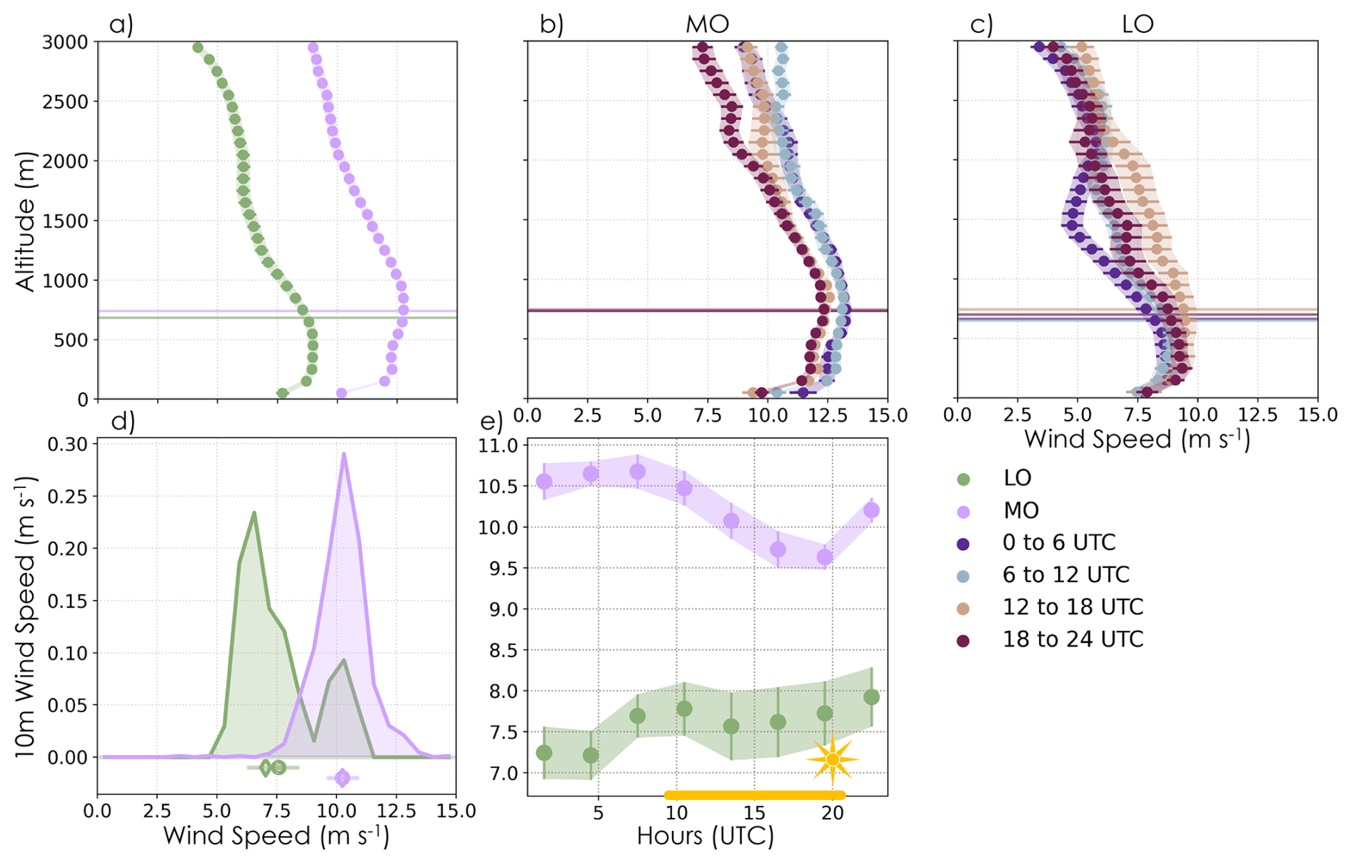
Figure 9 MO (purple and b) and LO (green and c) composites of radiosonde horizontal wind speed (a–c) and surface wind speed at 10 m (d–e). Mean profiles are composited absolutely (a) and in UTC ranges (b–c). Absolute PDF and statistical comparisons for surface wind speed are shown in panel (d) with mean (circle), median (diamond), 2 SE (thick line), and 25 %–75 % (thin line) statistics. The corresponding diurnal cycle is shown in panel (e). (a–c, e) Shading and lines represent 2 SE in the mean (circles), and filled circles are where the MO and LO distributions are different at 95 % confidence based on the Mann–Whitney U test. Composite mean (horizontal line) and 2 SE (shading hidden by line) lidar CBH are shown for reference (a–c).

Wind speed increases sharply from the surface, then stays relatively constant until above the mean CBH (horizontal lines) where it begins to decrease with height (a). This indicates there is no shear in the sub-cloud layer 100 m above the surface, allowing plumes to develop with limited interference for both MO and LO. Backwards shear manifests in the cloud layer and above: ∼ 2 m s⁻¹ km⁻¹ between 1 and 3 km (typical for this season in the trades, e.g., Helfer et al., 2020). Shear has a small amount of diurnal variability but is statistically indistinct between MO and LO (not shown). Wind direction is dominated by westward flow with some diurnal variability (not shown). Directional variation is also seen with height (Savazzi et al., 2022), becoming more easterly and northerly (veering north for LO, while MO is maintained more southward).

The LO and MO composite profiles (b–c) and surface (e) winds are statistically distinct for all hourly ranges across the diurnal cycle. Notably, LO surface winds tend to increase gradually over the day, while MO winds are highest at night, declining over the day. This is consistent with 10 m wind speed cycles observed at the NTAS buoy for sugar and gravel, respectively, although MO has a higher magnitude and later peak than gravel (Vial et al., 2021). The gradual increase in LO surface wind peaks at the end of the day (18:00–24:00 UTC) before dropping overnight, similar to the subtle pattern in LO w_CB Core mean and variance (Fig. 5c, f). The MO wind speed profile and surface are largest overnight (00:00–12:00 UTC) before being minimized during the day (12:00–24:00 UTC). The end of this extended maximum aligns with the peak in MO w_CB Core mean and variance at 06:00–12:00 UTC (Fig. 5a–c, f).

The stark wind speed differences are translated into the heat fluxes (Fig. 10): MO PDFs are shifted to larger latent (LHF, a) and sensible heat fluxes (SHF, b) compared to LO. This is also true for their combined buoyancy flux (Fig. C1a–b, same PDF and cycle shape as SHF). We find that MO PDFs and diurnal cycle composites are statistically distinct from LO distributions. The shapes of the LHF and SHF diurnal cycles are more distinct than those of the wind speed (Fig. 9e), peaking for MO (05:00–10:00 UTC) and increasing to maximum for LO (∼ 07:30 UTC) at the end of the night. SHF has a sharper cycle and larger relative amplitudes compared to LHF, maintaining a magnitude offset between MO and LO, but their phases are more alike than for LHF.

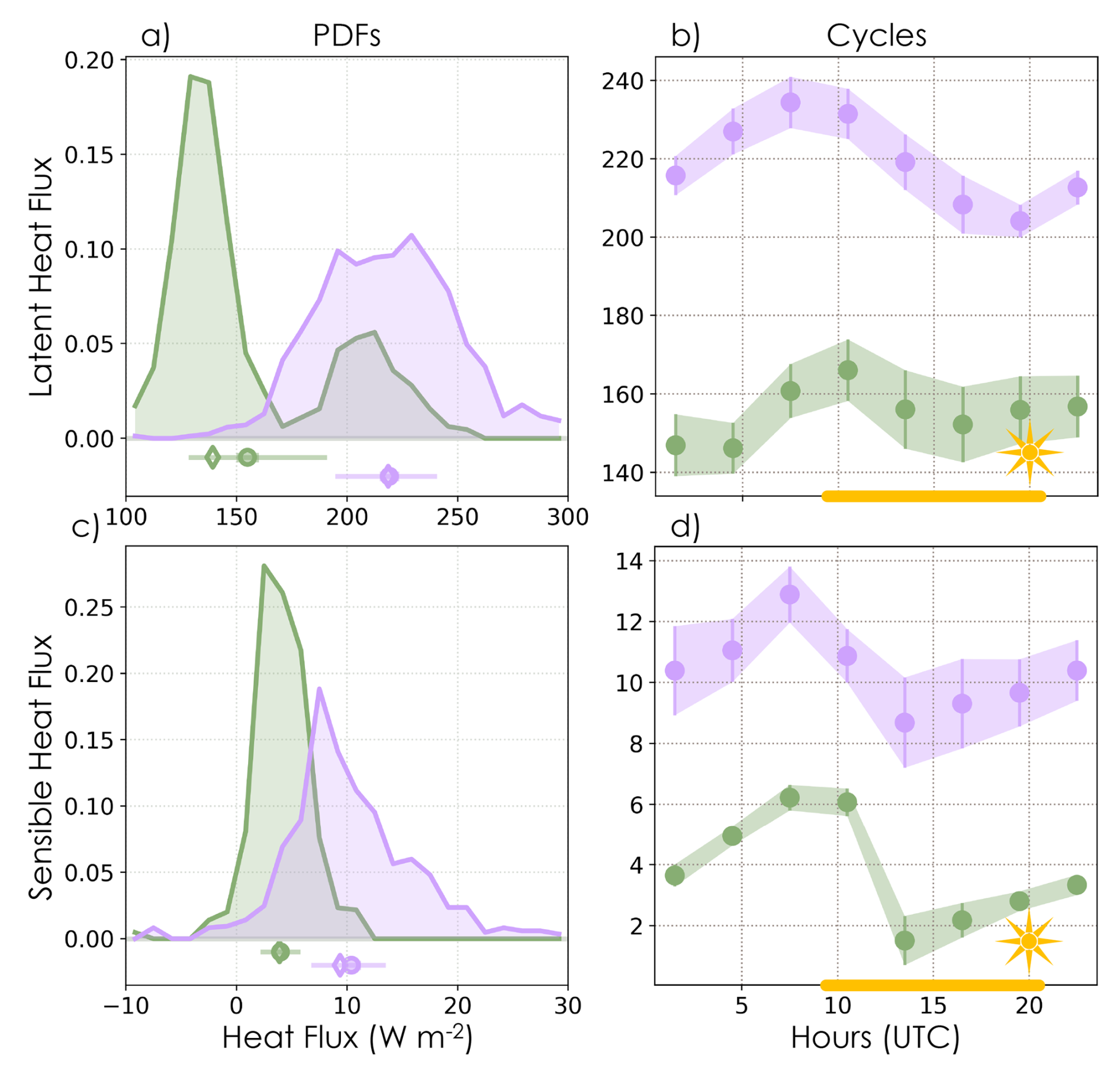
Figure 10 MO (purple) and LO (green) composite PDFs (a, c) and diurnal cycles (b, d) for latent (a–b) and sensible (c–d) heat fluxes. Variable statistics for each composite are shown below the PDFs: mean (circle), median (diamond), 2 SE (thick line), and 25 %–75 % (thin line). PDFs and diurnal cycle (filled circles) MO and LO distributions are different at 95 % confidence based on the Mann–Whitney U test.

The shapes of the LHF and SHF cycles are a result of the conflation between the air–sea temperature difference (Fig. C1d), surface humidity (Fig. 13e), and wind speed cycle (Fig. 9e). Air temperature responds more promptly to the diurnal cycle (increasing to maximum at ∼ 12:30 UTC, Fig. C2b), while sea surface temperature (SST) lags behind, likely due to a larger heat capacity, and is warmest at day's end and overnight (Fig. C2d). While the magnitudes are higher, these cycles are generally consistent with the climatological cycles seen for sugar and gravel (Vial et al., 2021). Their combination leads to an air–sea temperature difference that peaks at the end of the night and is at a minimum around ∼ 12:30 UTC for MO and LO (Fig. C1d). LHF has a more gradual cycle and follows wind speed more closely. LO and MO specific humidity at 10 m (q_10 m) is a minimum at the end of the night (Fig. 13e), aligning with the peak in wind speed and thus LHF. LO LHF is relatively constant over the course of the day, while MO LHF decreases at the end of the day before its nighttime increase.

MO LHF (SHF) is larger than for LO due to the combination of both larger magnitudes and diurnal cycle phase alignment between U_10 m and q_10 m (SST−T_10 m for SHF). The SHF and LHF early-morning peak matches the location of the MO w_CB Core variance peak and the beginning of the recovery from a nighttime lull in mean w_CB Core. There may be an accompanying increase in LO turbulence at CB, but it is not statistically distinct. This suggests that there is some boost to the updraft turbulence for MO, and possibly LO, from these turbulent energy fluxes. However, there is evidently another contributor to the MO cycle that helps to maintain the relatively constant MO w_CB Core during periods of declining fluxes and winds (Fig. 5a–c, f). The LO w_CB Core cycle, which holds steady but may peak at the end of the day, seems to align more with the larger daytime magnitudes in its associated wind and LHF cycles, suggesting some environmental support (c, d–f).

Thermodynamic profiles often modulate cloud systems' ability to develop and persist. We find that SST and T_10 m are both larger for LO and statistically distinct from MO cycles (Fig. C2b, d) and PDFs but not their interquartile range (a, c). These temperature differences are also consistent with the climatological separation between sugar (i.e., LO) and gravel (i.e., MO) (Bony et al., 2020; Schulz et al., 2021; Vial et al., 2021). Higher SSTs are often associated with increased dry-air entrainment and reduced low cloud amounts in stratocumulus regions (e.g., Klein et al., 2017; Scott et al., 2020). This appears to hold here as well (Fig. 6d). The combination of higher SST and smaller air–sea temperature differences and wind speeds, and thus smaller fluxes, likely damps LO plume strength and success (e.g., Fig. 6b, c). The MO–LO temperature offset extends through the depth of the BL with LO clouds tending to occur in warmer environments, with larger and statistically distinct potential temperatures compared to MO (Fig. 11a–c). LO cloud development is likely impaired through entrainment of warm, relatively drier air compared to MO (e.g., Fig. 13a, discussed more later). Note that both MO and LO sub-cloud layers are well mixed (i.e., constant θ with height until after CB), facilitating cloud development through even moisture distribution. MO θ profiles are relatively consistent across the diurnal cycle (b). However, LO above ∼ 1 km has a substantial diurnal cycle with θ increasing over the day (Fig. 11b), peaking at 18:00–24:00 UTC and being minimized at 06:00–12:00 UTC. This aligns with the T_10 m cycle but is a much larger magnitude (Fig. C2b). The relative magnitudes and cycles are consistent with θ profiles derived from reanalysis for sugar and gravel clouds (Vial et al., 2021).

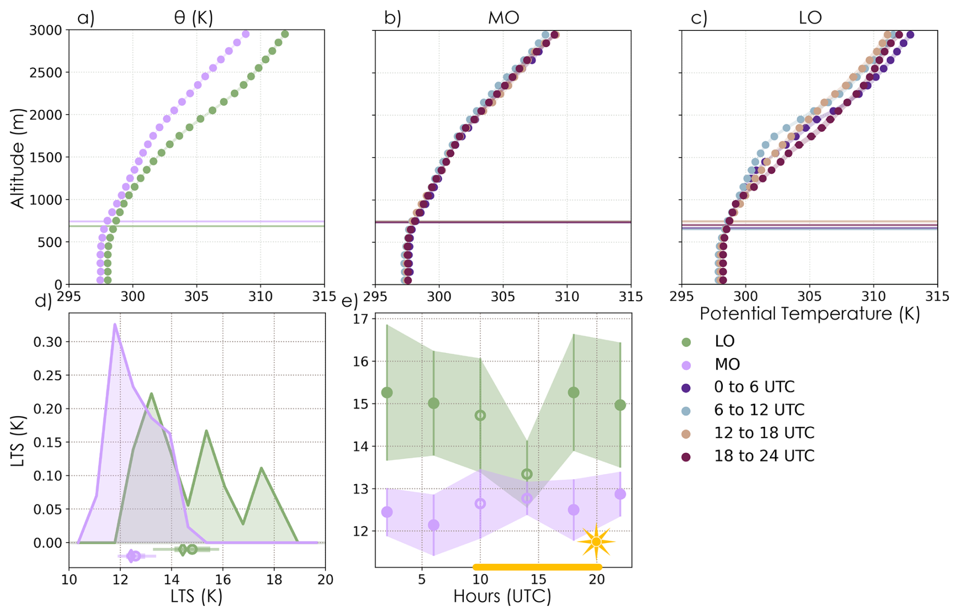
Figure 11 MO (purple and b) and LO (green and c) composites of radiosonde potential temperature (a–c) and lower-tropospheric stability (d–e). Mean profiles are composited absolutely (a) and in UTC ranges (b–c). Absolute PDF and statistical comparisons for LTS are shown in panel (d) with mean (circle), median (diamond), 2 SE (thick line), and 25 %–75 % (thin line) statistics. The corresponding diurnal cycle is shown in panel (e). (a–c, e) Shading and lines represent 2 SE in the mean (circles), and filled circles are where the MO and LO distributions are different at 95 % confidence based on the Mann–Whitney U test. Composite mean (horizontal line) and 2 SE (shading hidden by line) lidar CBH are shown for reference (a–c).

The amplification of the LO θ cycle above cloud may be associated with increased shortwave absorption from increased concentrations of absorbing aerosol on most of the LO days (recall LO on 30–31 January and 1, 4, and 9 February). Specifically, Quinn et al. (2022) identified a layer of absorbing aerosols aloft (29 January–3 February and 9 February) that were a mixture of biomass burning and dust transported from Africa to the RHB between 1 and 3 km in altitude. This aerosol layer gradually mixed into the BL as it was transported toward Barbados, increasing aerosol extinction throughout the atmospheric column and absorbing aerosol concentrations at the surface (e.g., Fig. C4a–c) (Quinn et al., 2022). 29–31 January and 1–3 February were the exception to this, with lower correlations between aerosol properties at the surface and aloft (Quinn et al., 2022). More absorbing aerosols aloft could increase the amount of shortwave absorbed over the diurnal cycle, heating above cloud and stabilizing the BL. Narenpitak et al. (2023) found in their LES study that the aerosol layer present on 31 January–2 February also deterred organization through longwave effects. During EUREC⁴A, low-level, longwave radiative cooling was found to depend on the ratio of relative humidity between the BL and FT and was influenced by moist intrusions at the mid-levels (Fildier et al., 2023).

Sub-cloud air temperature is more complicated to understand. There was no precipitation at the RHB during the LO period (Fig. C4d–e), enabling the aerosols to persist in the sub-cloud layer. If sufficient shortwave made it through the aerosol and cloud layers aloft, this could contribute to the larger LO T_10 m cycle (Figs. 11c, C2b). LO has lower total BL CF (Fig. A4d) along with higher surface humidity (Fig. 13a, c, e), potentially assisting in warming the sub-cloud more than for MO. The result of these effects may be the sharper daytime increase in LO LCL and thus CBH (Fig. C3a–b, horizontal lines in Fig. 11c), which would further deter cloud development. In contrast, the MO period was dominated by marine, non-absorbing aerosols (Quinn et al., 2022) that experienced some precipitation removal (e.g., coinciding with times of increased precipitation over the diurnal cycle, Fig. C4b, d–e), higher CF, and lower specific humidity, potentially damping any atmospheric heating signatures.

No matter the driver of the diurnal cycle in θ, it has a notable effect on the lower-tropospheric stability cycle (LTS = θ_700 hPa−θ_SLP, Klein and Hartmann, 1993, Fig. 11e). LO environments are more stable and statistically distinct from MO environments when examined in aggregate (d), consistent with the climatological sugar (i.e., LO) and gravel (i.e., MO) comparisons (Bony et al., 2020; Schulz et al., 2021). The MO and LO cycles are also similar to the gravel and sugar cycles, respectively, but have larger differences in magnitude and a less varied cycle for MO (Vial et al., 2021). Notably, MO and LO have the same stability at the beginning and middle of the day (∼ 10:00–15:00 UTC, e). This overlap corresponds to the period of increased winds (Fig. 9e) and fluxes (Figs. 10b, d, C1b) and occurs before re-stabilization of the LO BL, whose inversion appears to have degraded overnight.

Increased stability over the majority of the day presents an additional deterrent to LO clouds developing as their plumes will need to be sufficiently energetic to reach the simultaneously lifted LCL (Fig. C3a) and form a cloud. The brief drop in stability likely allows LO plumes to have some success early in the day, shortly after the winds and fluxes have peaked and more turbulent energy is available in the system. Similar behavior has been seen in the southeast Atlantic in the presence of smoke in the BL (Zhang and Zuidema, 2019). This also implies that persistent LO clouds are likely sub-selected for stronger w_CB Core that can better resist this environmental deterrence (Fig. 5c).

Even with this sub-selection, the stronger capping inversion for LO clouds may explain the flattening of the w_CB Core vs. L_CB Core curve (Fig. 8). Specifically, greater stability in LO will restrain clouds from deepening as much as in MO conditions, reducing their geometric depth (Fig. 12c) and liquid amount. We hypothesize that this damps their ability to release heat through condensation, which impairs both the local buoyancy enhancement from heating and the generation of mesoscale circulations, resulting in less updraft strengthening for LO clouds than MO clouds (Fig. 2a, b). The divergence between LO and MO curves grows with L_CB Core, consistent with deeper clouds being more enhanced. The opposite organization stability tendency has been shown in LES where a reduction in stability enhanced the transition from sugar to flowers and produced larger cloud features (Narenpitak et al., 2021). Further evaluation of the connection between environmental controls, dynamic efficiency, and mesoscale organization mechanisms is warranted. A more detailed evaluation of the LO evolution during the 30 January–2 February period at the RHB, highlighting the aerosol impacts mentioned here, is in development. The nuances of meteorology–aerosol covariability impacts on organized cloud systems, including the prevalence of LO clouds occurring under mixed dust and biomass burning aerosol conditions, is also worthy of future investigation (e.g., using the long record at BCO and following Zhang and Zuidema, 2019).

MO clouds exist in consistently more unstable environments (Fig. 11d–e), which is conducive to the development of deeper clouds and likely reinforces their moisture–convection feedback through facilitating lofting of humidity into the upper BL. A marker of the deeper MO clouds can be seen through comparing CBH measurements from the Doppler wind-lidar and the ceilometer (Fig. 12b–c). MO Doppler lidar CBH PDFs are shifted toward larger CBH and statistically distinct from LO. The mean and interquartile range overlap, though, with most CBH falling between ∼ 600 and 800 m for both (Figs. 12b, also 9a–c and sonde plots throughout). However, Doppler cloud identifications are restricted to have CBH near LCL (a), effectively removing any information about detraining cloud layers at the top of clouds or cloud edges as clouds tilt with height under shear. In contrast, the ceilometer CBH measurements are not restricted and capture a significant tail at upper levels for both MO and LO (Fig. 12c). This tail is more extensive for MO than LO, indicating that they consistently achieve greater heights (up to ∼ 2.5 km) compared to their less organized counterparts (∼ 1.5–1.8 km). Geometrically deeper clouds imply greater liquid water in the column and thus larger optical depth. Relative humidity profiles (Fig. C5) roughly support these cloud depths (Fig. 12c): 80 % until ∼ 2 km for MO and ∼ 1.3 km for LO on average. Merging of convective updrafts in organized tropical deep convection enables deeper clouds (Glenn and Krueger, 2017), consistent with the wider plumes and deeper extent of MO clouds. We also find that the total BL cloud amount (ceilometer measured CBH ≤ 3 km, Fig. A4d) is statistically larger for MO than LO (40 ± 4 % vs. 22 ± 6 %) despite their similar CB amounts, implying larger MO clouds potentially with detraining layers (a–c). Thus, MO clouds' greater dynamic efficiency likely supports a larger radiative impact due to their greater optical depth as well as their larger cloud amount (e.g., gravel vs. sugar, Bony et al., 2020). This potential connection between dynamic efficiency and impact on the radiation budget is worth investigating in future work.

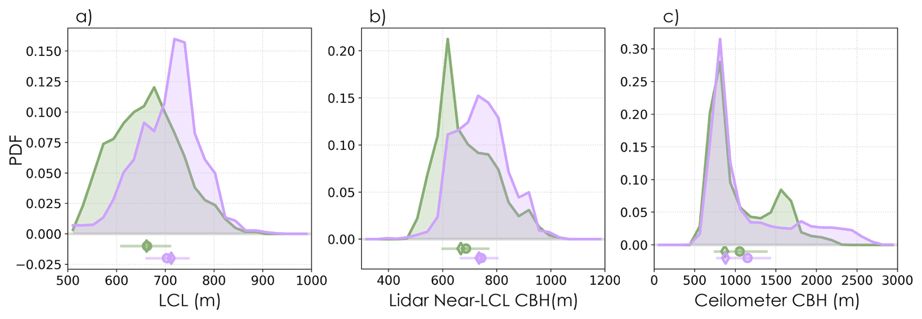
Figure 12 MO (purple) and LO (green) composite PDFs of (a) lifting condensation level (LCL), (b) Doppler lidar CBH for individual cloud scenes, restricted to within 50 m of the LCL, and (c) ceilometer CBH for shallow and mid-level clouds (below 3 km). Variable statistics for each composite are shown below the PDFs: mean (circle), median (diamond), 2 SE (thick line), and 25 %–75 % (thin line). The MO and LO distributions are different at 95 % confidence based on the Mann–Whitney U test.

To evaluate the prevalence of the moisture–convection feedback for MO cases and the type of air being entrained in both organizational states, we next examine the specific humidity profiles (Fig. 13). Unlike other variables, q has distinctly different organizational tendencies in the upper and lower BL (a). Above ∼ 1.3 km, MO q is much larger and from a statistically distinct distribution compared to LO. Moister FT (700 hPa) environments have also been seen for gravel (i.e., MO) than sugar (i.e., LO) (Schulz et al., 2021). Moisture advection likely does not explain the increased q aloft for MO vs. LO. The 3 d Lagrangian back trajectories of q_700 hPa are persistently drier for gravel than for sugar up until the final ∼ 12 h before the cloud observation (Schulz et al., 2021).

In the sub-cloud layer the opposite behavior is true: MO is substantially drier than LO below CB. This is particularly apparent in q_10 m (d–e). These statistically distinct separations hold across the diurnal cycle at the majority of altitude bins (b–c) and at the surface, with LO recovering more than MO by the end of the day (e). MO has a smaller magnitude than but similar diurnal cycle amplitude to LO at the surface and below CB, with both gaining the most moisture by the end of the day (18:00–24:00 UTC). MO q has a roughly similar diurnal cycle above CB as below (b). In contrast, LO q peaks by the end of the day in the sub-cloud layer and between 0:00 and 12:00 UTC in the middle BL. This may be linked to the period of greatest instability and largest fluxes, facilitating more active lofting of moisture (e.g., a minimum in q_10 m, e). A drier upper BL for LO clouds means that cloud-top entrainment will introduce more dry air than in MO clouds, additionally deterring LO cloud development. On the other hand, entraining moister air will help to maintain MO clouds for longer. Increased dry-air entrainment for LO clouds is also consistent with the previously discussed expectations associated with the higher SSTs for LO clouds.

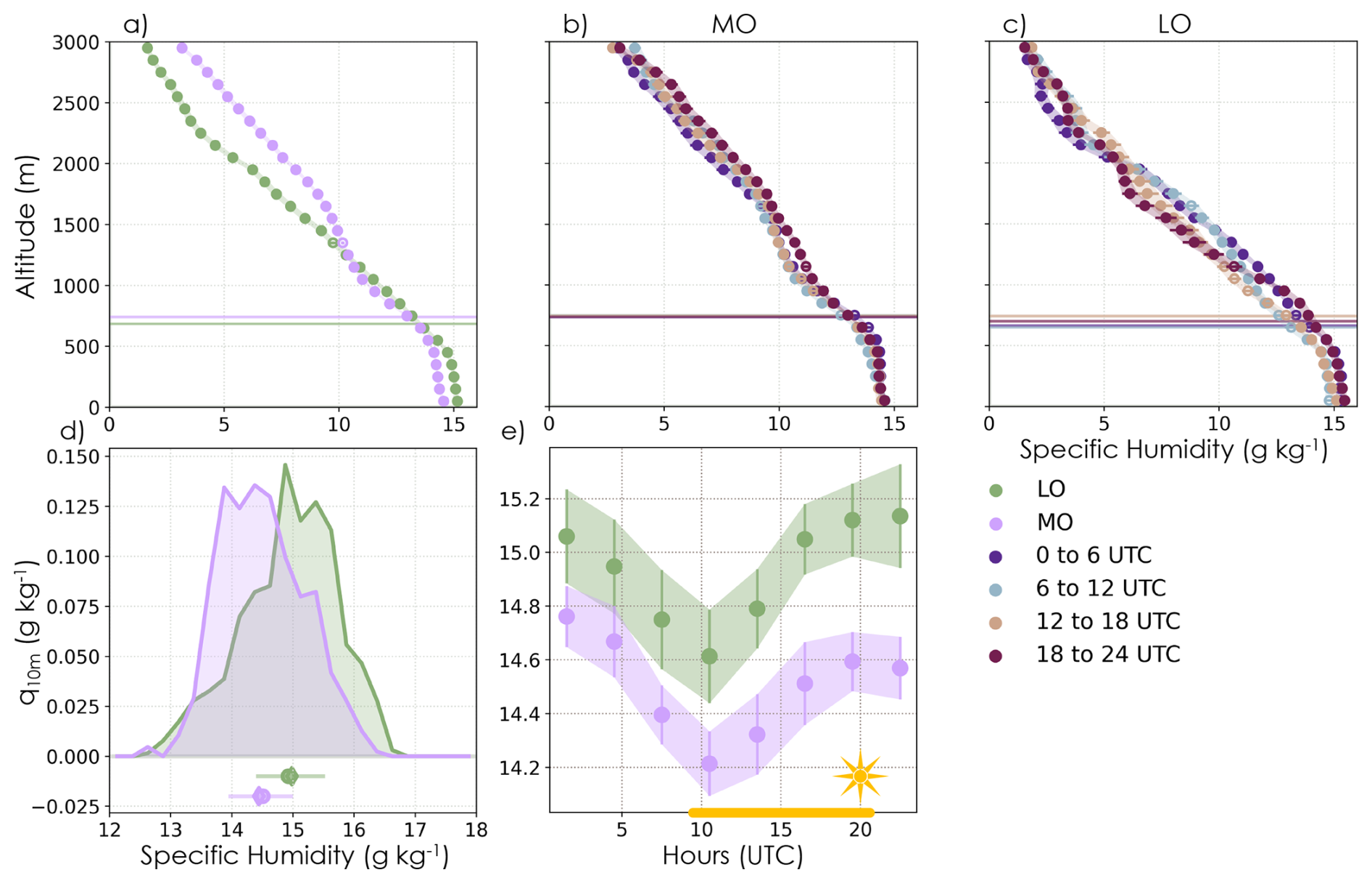
Figure 13 MO (purple and b) and LO (green and c) composites of radiosonde (a–c) and 10 m (d–e) specific humidity. Mean profiles are composited absolutely (a) and in UTC ranges (b–c). Absolute PDF and statistical comparisons for 10 m specific humidity are shown in panel (d) with mean (circle), median (diamond), 2 SE (thick line), and 25 %–75 % (thin line) statistics. The corresponding diurnal cycle is shown in panel (e). (a–c, e) Shading and lines represent 2 SE in the mean (circles), and filled circles are where the MO and LO distributions are different at 95 % confidence based on the Mann–Whitney U test. Composite mean (horizontal line) and 2 SE (shading hidden by line) lidar CBH are shown for reference (a–c).

The deeper and persistently moister layer aloft for MO is consistent with more moisture lofted into the upper BL through increased w_CB Core due to greater dynamic efficiency. This coincides with a critical part of the moisture–convection feedback, increasing aggregation of moisture into the ascending, cloudy branch as organization increases. Our analysis highlights a further nuance: the MO sub-cloud layer is drier than for LO clouds. This presents an additional barrier for MO clouds as it raises their LCL compared to LO clouds (Figs. 12a, C3a). The relative decoupling index (CBH–LCL/LCL, Kazil et al., 2017; Jones et al., 2011) is marginally higher for MO than LO although it is less diurnally variable (Fig. C3d). However, the average relative decoupling instances are both well below 0.1, indicating that MO and LO are both well coupled to the surface and that this is a small albeit statistically significant disadvantage. While the challenge for MO clouds to develop may be marginally increased, this could be ultimately helpful for increasing the strength of the CB updrafts (e.g., environments with higher LCL have wider, deeper, and stronger cloudy updrafts, Mulholland et al., 2021). In summary, the opposing q tendency in the upper and lower BL across organizational states is potentially an indication of the efficiency of moisture export to the upper BL through the stronger MO cloud updrafts, which more effectively remove sub-cloud moisture over time compared to the LO clouds. Note that on average the more organized systems downwind near Barbados exhibit the theoretically expected moisture enhancement throughout their ascending circulation branches including sub-cloud (George et al., 2023). Contrasting cloud organization stages and their vertical moisture behavior could provide insights into processes dominating mesoscale evolution, i.e., between early stages dominated by local cloud processes and “dynamic efficiency” (MO, Fig. 2b) vs. later stages where mesoscale circulations have strengthened enough to enhance moisture throughout the column and restore any previous depletion sub-cloud (Fig. 2c).

4 Discussion

It is evident from this analysis that there are organizational differences in the dynamics of trade wind Cu and that organization modifies the fundamental relationship between CB cloud amount and mass flux. Specifically, we have demonstrated that clouds with more mesoscale organization are dynamically more efficient: wider plumes produce stronger CB core updrafts through a given core size. We also show that these organizational differences increase with the size of cloud cores and are likely self-maintained by cloud-layer-driven circulations (i.e., mesoscale circulations developed from gravity ways triggered by heat release from condensation, Fig. 2), staying relatively resistant to diurnally varying environmental factors. Increased dynamic efficiency has important implications for MO clouds as they form: stronger updrafts through a given core result in more mass and moisture moved into the cloud system and the upper BL, increasing its moisture over time. Cloud-top entrainment will introduce moister air, helping to sustain MO clouds. This is consistent with the proposed mesoscale organization mechanism known as the moisture–convection feedback, which converges water vapor into the circulation's ascending, cloudy branch and strengthens the overturning circulation proportional to the updraft strength (e.g., Bretherton and Blossey, 2017; Janssens et al., 2023, 2024). The increased strengthening of updrafts near the cloud layer is supportive of cloud-layer-driven circulations being essential in this process (Narenpitak et al., 2021).

Our results are the first observational demonstration that mesoscale organization modifies CB mass flux through impacting updrafts. This is a divergence from the idea that CB mass flux primarily depends on CB cloud amount, an important assumption in mass budget analyses (e.g., Klingebiel et al., 2021; George et al., 2021; Vogel et al., 2022). The closure arguments utilized in these studies produce reasonable mass fluxes that vary with environmental conditions, outperforming current GCM parameterizations in capturing Cu behaviors (e.g., Vogel et al., 2022). However, our results indicate that the organizational modulations of updraft strength and thus mass flux are important processes that may be missing from this framework. The greater dependence of mass flux on dynamic factors (e.g., mesoscale vertical velocity) in Vogel et al. (2022) may be an indication that the organizational contributions are being aliased in, accounting for the increased dynamic efficiency of organized clouds. By definition, all variability not captured by the other budget terms must go into the mass flux closure. However, explicitly accounting for the contribution from updraft strengthening as mass flux increases with organization would provide a key process-level insight for Cu development, informing our understanding of how organization modifies clouds in the trades even from their earliest development stages. Recent work indicates that this contribution becomes increasingly important as Cu organizes: cloud-associated velocity variations have an increased contribution to CB mass flux under strengthening mesoscale ascent (Janssens et al., 2024). Janssens et al. (2024) evaluations include a broader range of cloud structure sizes in their simulations, while we focus on relatively small structures, early in their evolution across the Atlantic basin. However, the clear organizational differences already apparent in our results indicate that such differences will persist and likely grow larger as cloud systems evolve and grow in structure size across the basin, continuing to undergo mesoscale organization. Our results encourage future evaluations expanding this analysis to a longer observational record, larger organizational scales, and other mass flux calculation frameworks.

Eventually, it is likely that the dynamic efficiency facilitating the moisture–convection feedback loop will be broken once clouds are sufficiently organized to precipitate. The accompanying cold pools that are generated along with their associated downdrafts will reverse the circulation direction, breaking the feedback cycle. The dynamic efficiency may also slow with time as the sub-cloud layer moisture is depleted. The small cloud structures examined here have limited (MO) to no (LO) precipitation (Fig. C4d–e) and thus no cold pools (rarely seen at the RHB, Touzé-Peiffer et al., 2022). These results are thus applicable to the development stage of the cloud cycle rather than the decay. However, we do see that the MO vs. LO cloud-topped plume width and cloud size distributions (Fig. 6b, d–e) are consistent with the oscillations in cloud size and thermals in the literature that evolve between states with relatively more small clouds (e.g., LO) and states with relatively more large clouds (e.g., MO) (Feingold et al., 2017; Oh and Austin, 2024). These oscillations are driven by aggregation of small clouds and thermals into larger clouds and thermals before breaking up, operating on a faster timescale (1.5 to 2 h, Feingold et al., 2017; Oh and Austin, 2024) than the mesoscale organization that is likely influencing the separation here (e.g., 12 h to a day, Narenpitak et al., 2021). However, it is a useful behavioral comparison to make against the eventual evolution of the clouds through their organizational states: LO to MO to eventual collapse and return to LO. This type of organizational cycling may further influence the energetic discharge–recharge cycle: the MO dynamic efficiency phase could potentially moisten the cloud and upper BL enough to enable the transition from the shallow to the deep cycle, kicking off deep convection development (Wolding et al., 2024). Investigating the full cloud life cycle would require examination of LES or geostationary satellite analysis.

None of the tested cloud controlling factors sufficiently explained the persistence of MO CB core updrafts and amount across the diurnal cycle. Nor was there such a factor controlling the sub-cloud enhancement of MO updrafts, which occurred more with increasing core size. Instead, cloud-layer-driven circulations operating as part of the mesoscale moisture–convection feedback may help to sustain MO clouds once they are formed through reinforcing plumes and strengthening w_CB Core. Such coupling and reinforcement between mesoscale cloud patterns, cloud-layer-driven circulations, and increased vertical transport of momentum and moisture through the sub-cloud layer have been seen historically (e.g., LeMone and Pennell, 1976). There has also been a climatological shift toward more frequent occurrences of Sc-like clouds in this region (i.e., MO) (Eastman et al., 2025), which is projected to continue under future SST and stability changes (McCoy et al., 2023), leading to a negative feedback associated with cloud morphology that may suppress Caribbean warming and drying (Eastman et al., 2025; McCoy et al., 2023). Taken together, these results have important implications for future trade Cu: climatologically more frequent MO clouds may be less susceptible to environmental perturbations as their moisture–convection feedback may be more resilient to environmental changes. However, a recent LES case study showed that increased greenhouse gases under future conditions damp mesoscale circulations in the larger, more organized flowers clouds, leading to a more positive tropical Cu feedback (Kazil et al., 2024). The multi-scale complexity of these mesoscale systems encourages continued examination of organization influence on vertical velocity profiles and the resulting cloud system sensitivity to environmental conditions. This is especially important to undertake in order to improve Cu representation in GCMs for robust climate projections.

5 Summary

In this study, we utilized a unique, shipborne observational dataset taken in the wintertime trades upwind of Barbados during the 2020 ATOMIC (Quinn et al., 2021) and EUREC⁴A (Stevens et al., 2021) joint campaigns. Our primary source of data was a motion-stabilized Doppler wind-lidar aboard the RV Ronald H. Brown that we used to examine the dynamics of trade Cu and their associated plume behaviors. We additionally used thermodynamic and environmental measurements collected on board and from ship-launched radiosondes. These observations were composited based on hand-identified classifications into more (MO) and less (LO) organized boundary layer cloud structures on the mesoscale (O(100 km)). Organization classifications were validated against objective measures of mesoscale clustering (following Bony et al., 2020), indicating that MO and LO have similar cloud structure sizes but substantially different degrees of clustering.

We find that MO clouds have larger and statistically distinct updraft vertical velocity mean and variance compared to LO clouds. This holds across ranges of cloud-base (CB) core size and the diurnal cycle. Updraft strength increases with CB core size for both MO and LO but the organizational difference widens substantially. MO cloud updraft strength increases without apparent constraint, while LO clouds plateau at larger core sizes, potentially due to capping from their larger tropospheric stability, impairing cloud deepening and limiting condensation, which would reduce local buoyancy production and limit mesoscale circulations. The increases in MO updraft strength with core size particularly manifest in their upper sub-cloud layer, implying that cloud-layer-driven circulations associated with condensational heat release may be reinforcing cloud updrafts. Unsuccessful, clear-sky plumes are similar across organizational states, but MO cloud-topped plumes succeed at a much higher rate with increasing plume width, further pointing to cloud-driven processes reinforcing organizational differences in dynamics. MO clouds tend to have wider cloud-topped plumes than LO but MO and LO have the same positive relationship between plume width and core size. However, the positive cloud-topped plume width relationship with CB core updraft strength is significantly stronger for MO than LO clouds and statistically distinct. We conclude that MO clouds have greater dynamic efficiency than LO clouds: organized sub-cloud and CB core updrafts are substantially stronger for a given plume width, and thus core size, leading to larger CB mass flux for organized clouds.

MO and LO environments are statistically distinct, helping to shape their cloud development and persistence. There is not a robust cycle in MO or LO CB core updraft mean or variance. Fluxes contribute to a peak in MO CB turbulence at the end of the night. LO CB core updraft consistency may have had some support from heightened turbulent surface fluxes and wind speed during the day. This also coincides with increased sub-cloud warming over the day, potentially energizing the thermal plumes that drive these more environmentally coupled clouds. LO clouds may sub-select for stronger updrafts to overcome daytime (and potentially absorbing aerosol-induced) stability and lifting condensation level increases. However, LO CB cloud amount does drop over the day, indicating some cloud depredation despite this sub-selection. MO clouds have higher wind speed and fluxes and lower stability environments on average, facilitating deeper clouds. Their sub-cloud and CB core updrafts, as well as cloud amount, were persistent and not significantly assisted or deterred by diurnally varying environmental factors (particularly flux and wind speed reductions over the day). This lack of diurnal coupling additionally supports the idea of cloud-layer-driven circulations maintaining MO clouds once they have been formed (consistent with limited surface contributions to mesoscale organization, i.e., Janssens et al., 2024). Notably, MO clouds have much higher specific humidity in and above the cloud layer and lower humidity sub-cloud compared to LO clouds. This, along with the deeper and wider extent of MO clouds in the BL, is likely a marker of the mesoscale moisture–convection feedback taking effect in MO clouds. Increased dynamic efficiency of MO clouds imports more moisture into the cloud layer and upper BL. This leads to reduced sub-cloud moisture over time and helps maintain MO clouds through moistening air entrained at cloud top.

The organizational differences in cloud efficiency identified in this study likely play a fundamental role in the moisture–convection feedback intrinsic to the process of mesoscale organization, enabling MO cloud persistence and furthering mesoscale organization of trade Cu (e.g., Fig. 2). We have observationally demonstrated for the first time that organization impacts CB mass flux through modulating updrafts, a departure from the expectation that mass flux is controlled by CB cloud amount (e.g., Klingebiel et al., 2021; George et al., 2021; Vogel et al., 2022). Our results are consistent with recent modeling evidence of mesoscale cloud velocity variability becoming increasingly important under greater mesoscale ascent (Janssens et al., 2024) and greater dynamic dependence in mass flux (Vogel et al., 2022). Greater dynamic efficiency in MO clouds likely facilitates the energetic discharge–recharge cycle that controls precipitation in the tropics, increasing the amount and depth of moisture in the BL that initiates the transition from shallow to deep convection (Wolding et al., 2024). We hypothesize that MO clouds, once established, are driven more by cloud layer circulations and are resilient to diurnal changes in environmental controls. This has important implications for the potential susceptibility of MO clouds to climate change. Combined with the trend toward MO clouds in the Caribbean since 1971 (Eastman et al., 2025), our results suggest that tropical Cu clouds may be more resilient to future environmental changes than previously thought due to their tendency toward increased mesoscale organization. These results encourage the continued assessment of mesoscale organization impacts on the climate system and evaluation of whether representing their characteristics in GCM parameterizations is valuable for reducing future climate uncertainty.

Appendix A: Cloud organization identifications

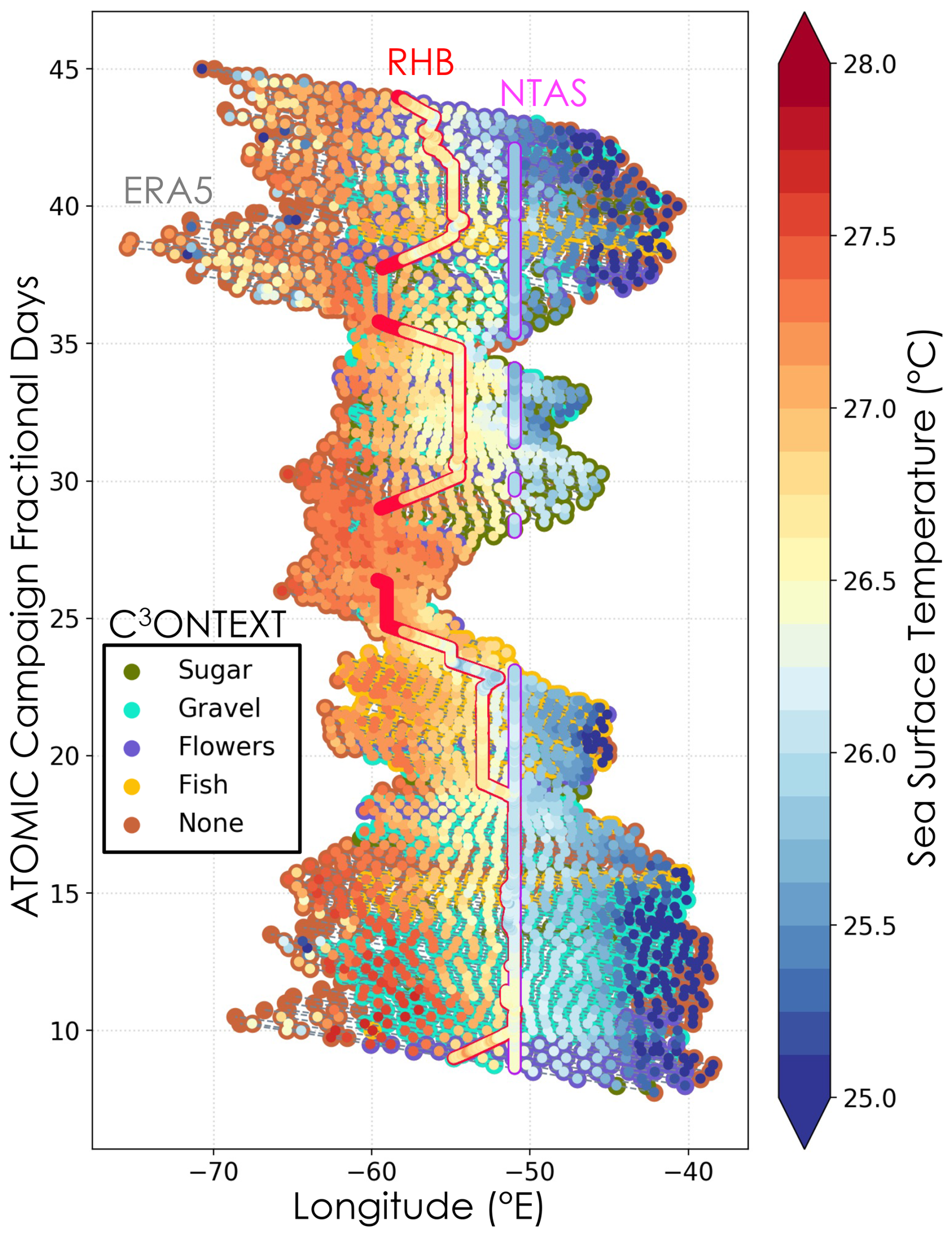
Figure A1 Hovmüller diagram of cloud organization evolution during ATOMIC. Dashed lines are 30 h forward and 30 h backward Lagrangian trajectories originating from the RV Ronald H. Brown (c/o Ryan Eastman). ERA5 sea surface temperature is extracted at each 3 h point along the trajectories. Observations within 100 km and 3 h of a trajectory point are extracted and overplotted for the RHB (red) and NTAS (Plueddemann et al., 2021) (pink) platforms. Morphology patterns are identified for each trajectory point from C³ONTEXT (Schulz, 2022a) and plotted behind observations. If the point cannot be confidently labeled (i.e., fraction ≤ 50 %), it is marked as “none”.

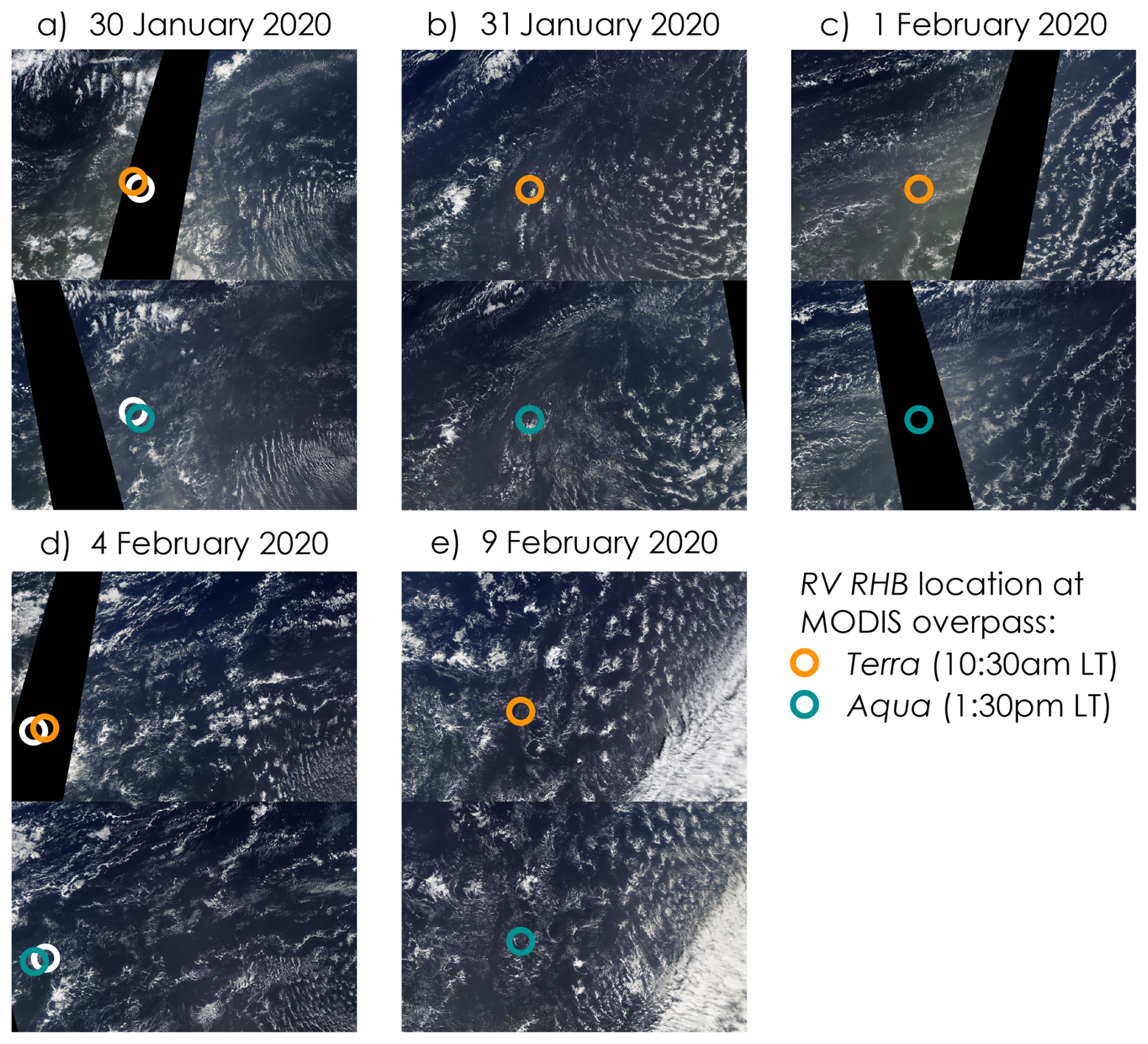
Figure A2 LO cases (10–20° N, 60–45° W) selected based on visual assessment of RV RHB platform locations during MODIS Terra (orange, 10:30 LT) and Aqua (green, 13:30 LT) overpasses. Circles represent locations of RHB at overpass times. White circles mark the location of the other overpass time, indicating when the RHB was moving.

Figure A3 MO cases as described in Fig. A2.

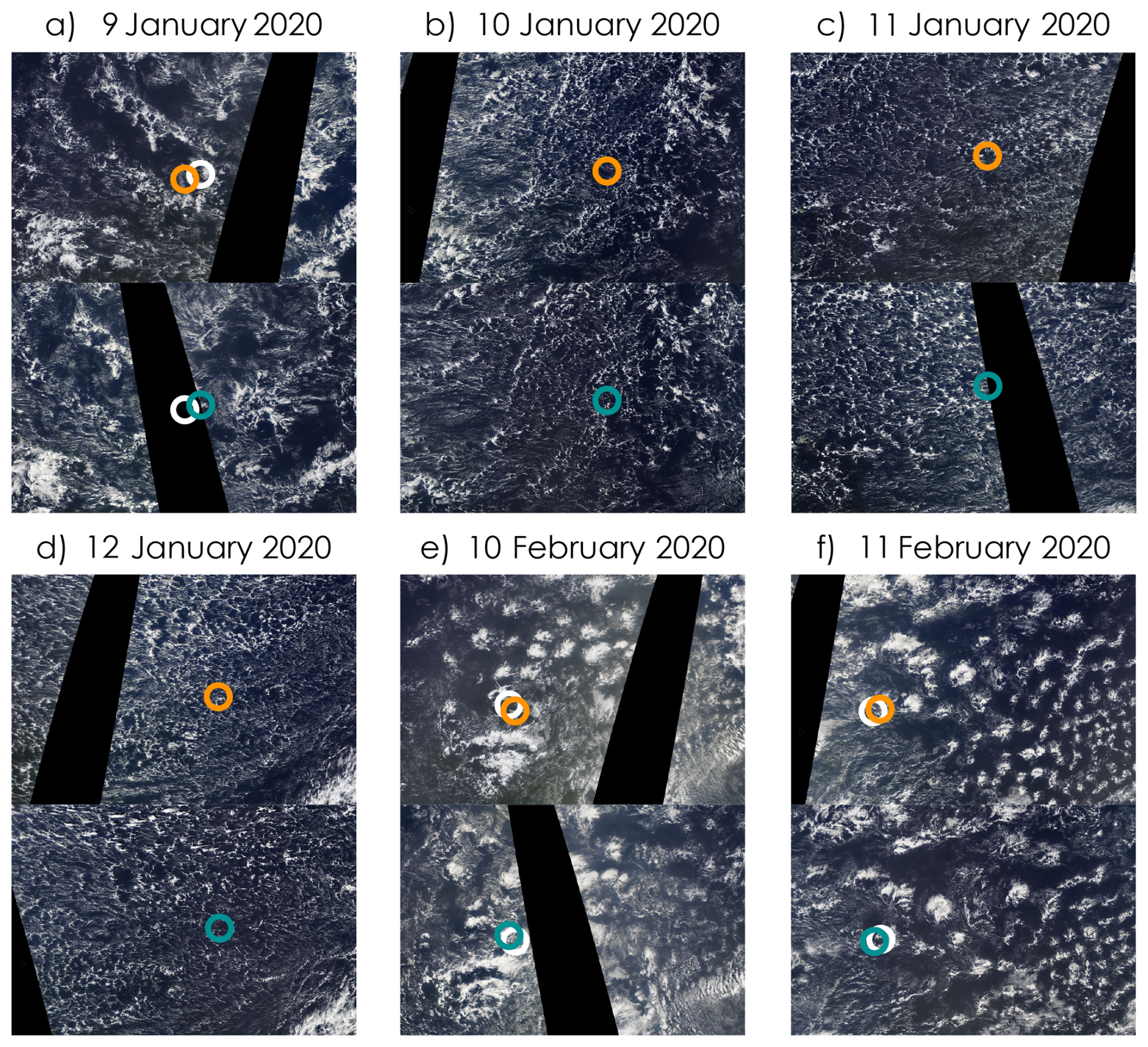
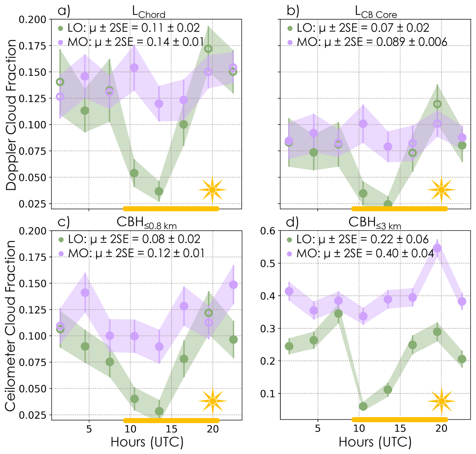
Figure A4 MO (purple) and LO (green) composite diurnal cycles of cloud fraction computed using identifications from the Doppler wind lidar cloud duration for chord length (a) and core length (b) and from the ceilometer for approximate CB (c, CBH ≤ 800 m) and total BL (d, CBH ≤ 3 km). Filled circles indicate where MO and LO distributions for a given 3 h bin are different at 95 % confidence based on the Mann–Whitney U test. Doppler wind lidar estimates are derived from the duration (in seconds) scaled by the number of observations averaged into a given bin divided by the total number of observations over the composite. Diurnal mean and 2 SE are provided for reference.

Appendix B: Dynamic efficiency of organized clouds

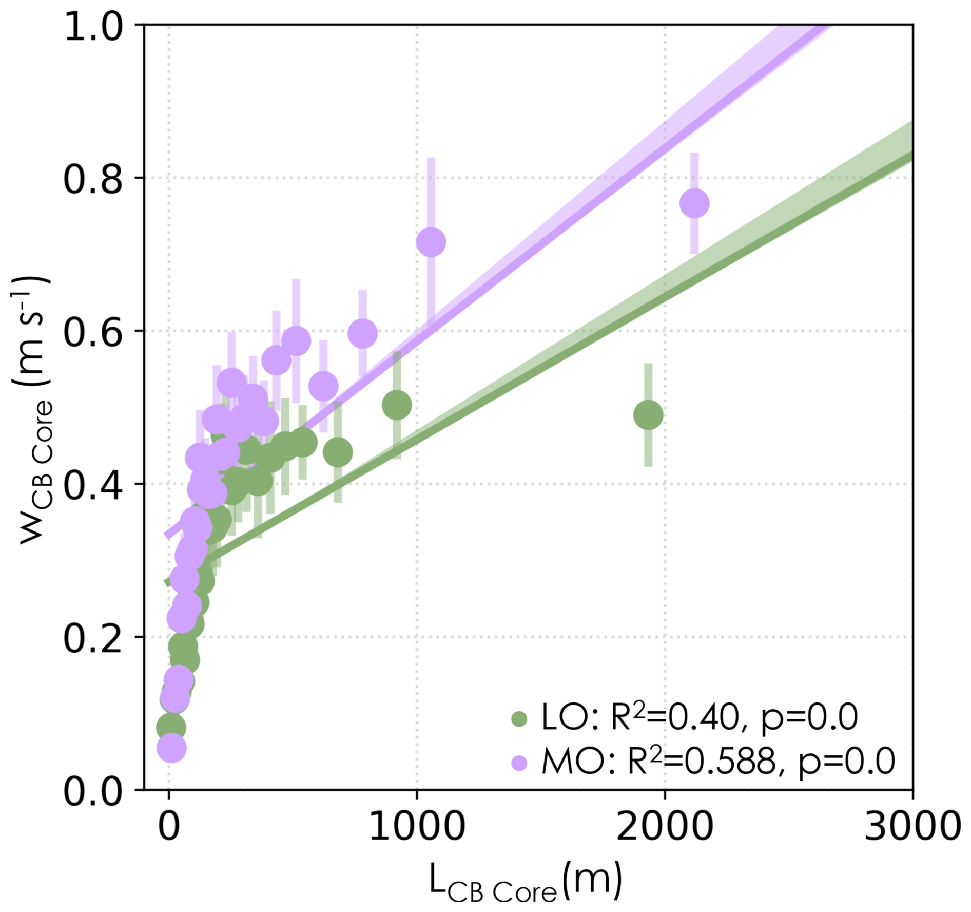
Figure B1 MO (purple) and LO (green) composites of CB core size (L_CB Core) vs. velocity (w_CB Core). Best-fit linear regressions are computed on the underlying data with confidence intervals (min and max, shading) calculated using the jackknife method (Tukey, 1958). Mean (dot) and 2 SE (vertical lines) of w_CB Core are plotted in quantiles of L_CB Core to illustrate the distribution of data. Correlation coefficients for quantile relationships are significant at 95 % confidence.

Appendix C: Characteristics of organized environments

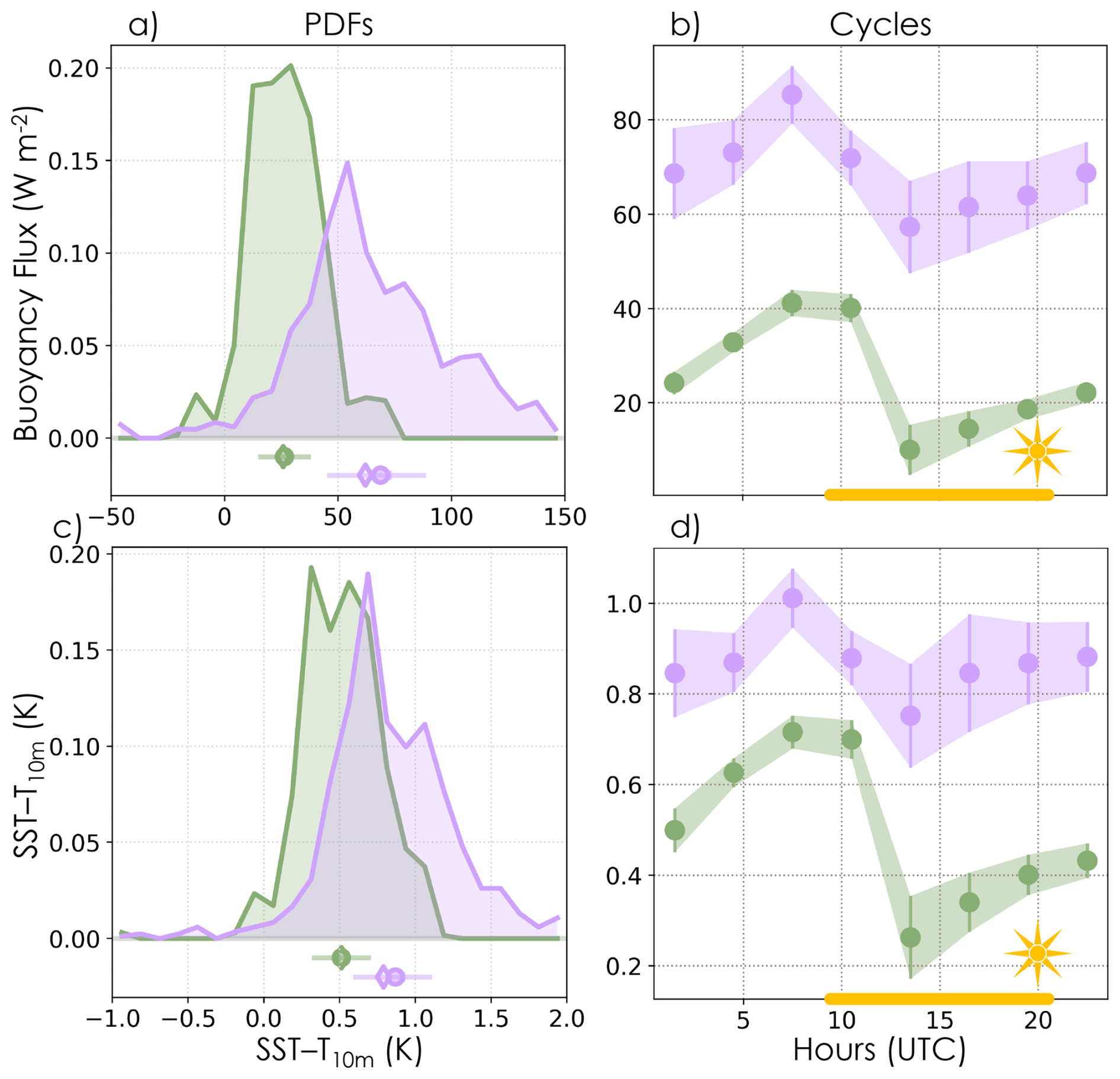
Figure C1 MO (purple) and LO (green) composite PDFs (a, c) and diurnal cycles (b, d) for buoyancy flux (a–b) and temperature difference between the sea surface and 10 m air (c–d). Variable statistics for each composite are shown below the PDFs: mean (circle), median (diamond), 2 SE (thick line), and 25 %–75 % (thin line). PDFs and diurnal cycle (filled circles) MO and LO distributions are different at 95 % confidence based on the Mann–Whitney U test.

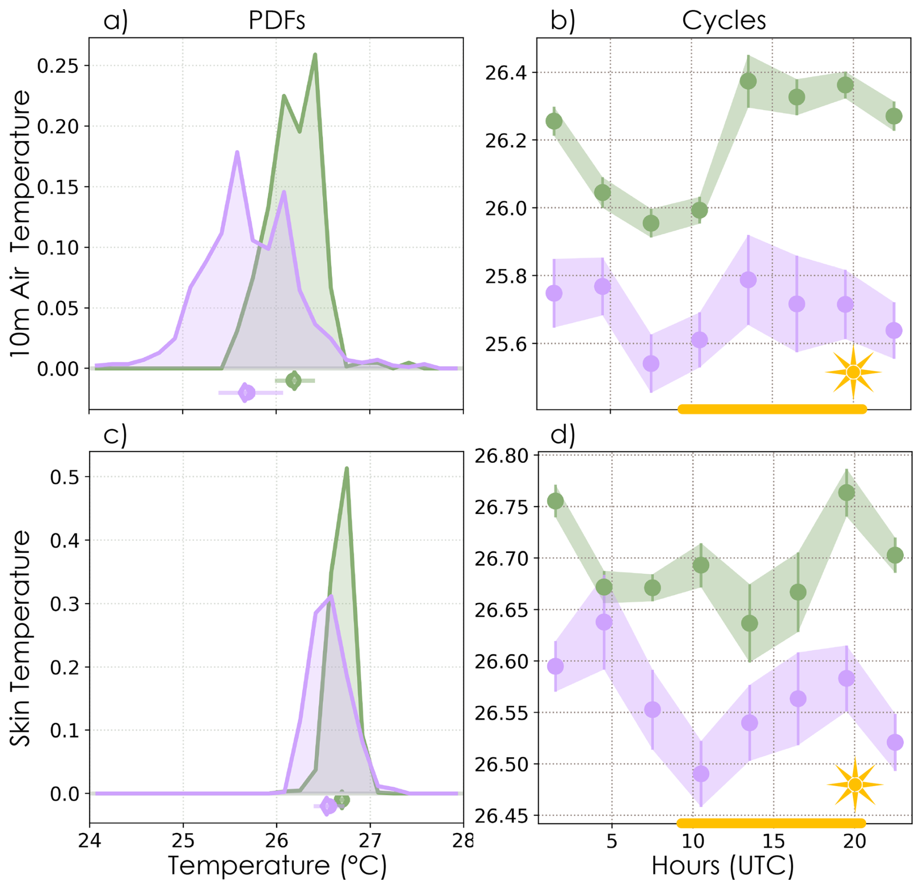
Figure C2 MO (purple) and LO (green) composite PDFs (a, c) and diurnal cycles (b, d) for 10 m air (a–b) and sea surface skin (c–d) temperatures. Variable statistics for each composite are shown below the PDFs: mean (circle), median (diamond), 2 SE (thick line), and 25 %–75 % (thin line). PDFs and diurnal cycle (filled circles) MO and LO distributions are different at 95 % confidence based on the Mann–Whitney U test.

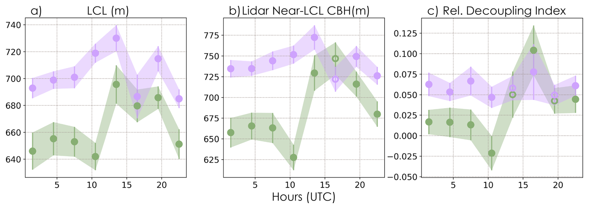
Figure C3 MO (purple) and LO (green) composite diurnal cycles for lifting condensation level (a), near-LCL CBH (b), and relative decoupling index (c) for individual cloud observations from the lidar. Mean (dot) and 2 SE (vertical lines, shading) are shown for each hour range. MO and LO distributions (filled circles) are different at 95 % confidence based on the Mann–Whitney U test.

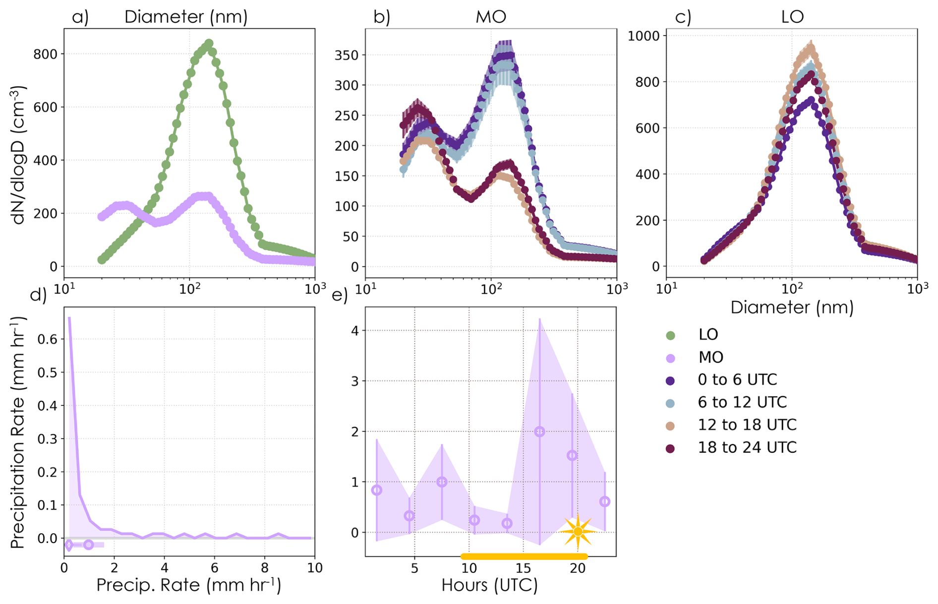
Figure C4 MO (purple and b) and LO (green and c) composites of merged and lognormal fitted DMPS and APS (Quinn et al., 2022) number distributions (a–c) and precipitation rate (d–e). Mean distributions are composited absolutely (a) and in UTC ranges (b–c). Absolute PDF and statistical comparisons for precipitation rate are shown in panel (d) with mean (circle), median (diamond), 2 SE (thick line), and 25 %–75 % (thin line) statistics. The corresponding diurnal cycle is shown in (e). Note that precipitation only occurred during MO periods, which appear to help deplete accumulation-mode aerosol during hours of more frequent precipitation (12:00–24:00 UTC). (a–c, e) Shading and lines represent 2 SE in the mean (circles), and filled circles are where the MO and LO distributions are different at 95 % confidence based on the Mann–Whitney U test.

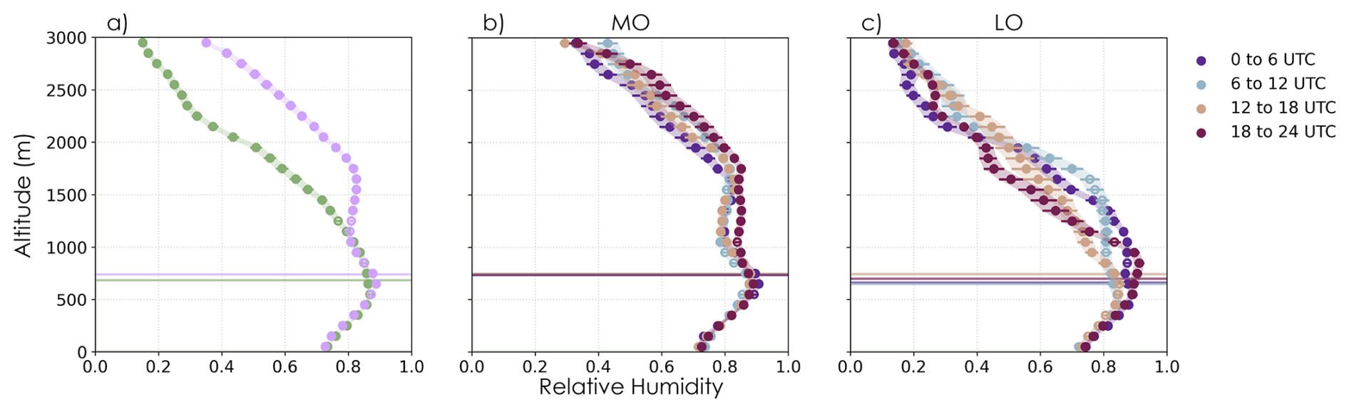
Figure C5 MO (purple and b) and LO (green and c) composites of radiosonde relative humidity (a–c). Mean profiles are composited absolutely (a) and in UTC ranges (b–c). Shading and lines represent 2 SE in the mean (circles), and filled circles are where the MO and LO distributions are different at 95 % confidence based on the Mann–Whitney U test. Composite mean (horizontal line) and 2 SE (shading hidden by line) lidar CBH are shown for reference (a–c).