Measurement report: Eight years of greenhouse gas fluxes at Saclay, France, estimated with the Radon Tracer Method

Here, we use carbon dioxide (CO₂), methane (CH₄), carbon monoxide (CO), nitrous oxide (N₂O) and radon (²²²Rn) data from the Saclay ICOS tall tower in France to estimate CO₂, CH₄ and CO fluxes within the station footprint from January 2017 to October 2024 and N₂O fluxes from February 2019 to October 2024 using the Radon Tracer Method (RTM).

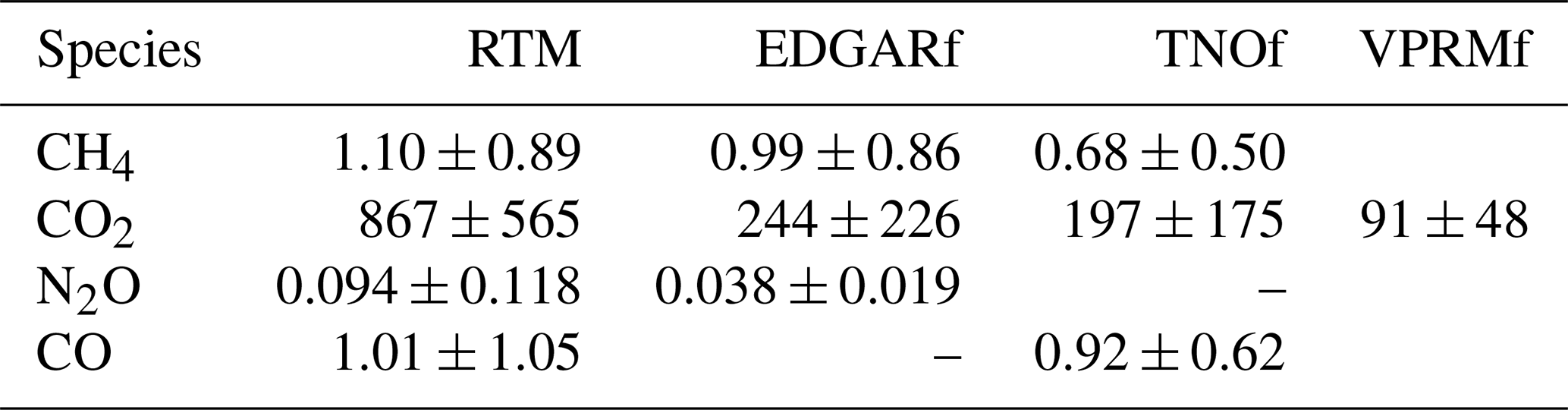
We first performed a sensitivity study of this method applied to CH₄ and combined with different radon exhalation maps including the improved European process-based radon flux maps developed within 19ENV01 traceRadon and back-trajectories in order to optimize it. Then, radon exhalation maps from the 19ENV01 traceRadon project, STILT trajectories from the ICOS Carbon Portal, best estimate of radon activity concentration and greenhouse data have been used to estimate the surface emissions. To our knowledge, this is the first study in Europe using the latest radon exhalation maps and standardized radon measurements to estimate CO₂, CH₄, CO and N₂O surface emissions. We found that the average RTM estimates are 867 ± 565, 1.10 ± 0.89, 1.01 ± 1.05 and 0.094 ± 0.118 $\mathrm{mg}{\mathrm{m}}^{-\mathrm{2}}{\mathrm{h}}^{-\mathrm{1}}$ for CO₂, CH₄, CO and N₂O, respectively. These fluxes are in good agreement with the literature for the same site or for similar suburban sites in Europe. No significant trends are observed over time, except for CO, which shows a small decreasing trend especially over the last three years.

CH₄, N₂O and CO are also in fair agreement with the inventories, though with higher values. CO₂ fluxes are about 5 times higher than modeled anthropogenic and biogenic fluxes combined. The differences mainly occur during summer, and the $\mathrm{CO}/{\mathrm{CO}}_{\mathrm{2}}$ ratio points toward a misrepresentation of the biogenic fluxes by the WRF-VPRM version used here.

1 Introduction

Precise greenhouse gas monitoring began with CO₂ in the 1960s at background stations such as the South Pole and the Mauna Loa Observatory (Keeling, 1960; Brown and Keeling, 1965; Pales and Keeling, 1965). Since then, CO₂ as well as other greenhouses gases (GHG) such as CH₄ and N₂O levels have risen significantly in the atmosphere. To monitor these changes, measurement networks (Prinn et al., 2018; Andrews et al., 2014; Fang et al., 2014; Ramonet et al., 2010) and coordinating programs (WMO, 2014) have been developed worldwide and help disentangle the different roles of the biospheric fluxes, oceanic fluxes and anthropogenic emissions. Initially, background stations were set up to monitor long-term changes in hemispheric mean GHG amount fraction globally. However, in recent years, there has been a shift towards measuring regional and national amount fraction to verify and improve GHG emission assessments, known as ”bottom-up” methods. Bottom-up methods rely on aggregated activity data, emission factors, and facility-level measurements, but often have significant uncertainties, especially for non-CO₂ GHGs, due to varying emission factors across sectors and biases from unaccounted sources. This smaller scale is thus especially relevant in the context of monitoring and verifying the international climate agreements (Bergamaschi et al., 2018).

Within the existing networks, the Integrated Carbon Observation System (ICOS) is a pan-European research infrastructure (Heiskanen et al. (2021); Yver-Kwok et al. (2021), https://www.icos-ri.eu, last access: 16 October 2025) which provides highly compatible, harmonized and high-precision scientific data on the carbon cycle and greenhouse gas budget. It began with a preparatory phase from 2008 to 2013 and a demonstration period until 2015 when ICOS officially started as a legal entity. Three monitoring networks, atmospheric observations, flux measurements within and above ecosystems, and measurements of CO₂ partial pressure in seawater contribute to ICOS. To date, the atmospheric network consists of 39 stations located mostly in Europe (https://www.icos-atc.lsce.ipsl.fr/network, last access: 16 October 2025) and seven more stations will join the network in the years to come. Depending on station class (class 1 or 2), different parameters are mandatory or recommended for measurement. CO₂ and CH₄ are mandatory at all stations, CO is mandatory only for class 1, and N₂O and ²²²Rn are recommended observations (ICOS RI, 2020).

Combining regional atmospheric GHG measurements with atmospheric transport models provides an opportunity for independent “top-down” verification of GHG bottom-up estimates, known as inverse modelling (Bergamaschi et al., 2018). However, due to the significant uncertainties associated with atmospheric transport models, this method is not yet fully reliable for verification of GHG fluxes. An alternative independent method for verifying GHG fluxes is the observation-based Radon Tracer Method (RTM). This method, independent of an atmospheric transport model, is also relatively simple. RTM involves simultaneous measurements of radon (²²²Rn) and GHG at co-located sites, along with the estimation of a radon source function. Radon is particularly useful because it is a naturally occurring radioactive gas with a well-defined source (soil), a simple sink (half-life of 3.82 d), and chemical inertness. Due to these properties, radon can be used effectively as a tool for estimating and verifying GHG fluxes (Chambers et al., 2019; Kikaj et al., 2020; Zhang et al., 2021; Quérel et al., 2022). Indeed, like GHGs which usually have their sources close to the ground, ²²²Rn accumulates during the night within the lower boundary layer. Thus, both ²²²Rn and GHGs will accumulate together overnight and their correlation can be used to estimate the flux of GHG as long as we know the exhalation rate of ²²²Rn. The RTM has been used in many studies to evaluate the fluxes between the atmosphere and ecosystems of trace gases such as CO₂, CH₄, N₂O, H₂ or COS (e.g.: Levin et al., 1999; Schmidt et al., 2001; Biraud et al., 2000; Messager, 2007; Yver et al., 2009; Hammer and Levin, 2009; Lopez et al., 2012; Vogel et al., 2012; Belviso et al., 2013; Grossi et al., 2018; Belviso et al., 2020; Levin et al., 2021; Tong et al., 2023). For example, Levin et al. (1999) calculated an estimate of 0.8 $\mathrm{mg}{\mathrm{CH}}_{\mathrm{4}}{\mathrm{m}}^{-\mathrm{2}}{\mathrm{h}}^{-\mathrm{1}}$ for the Heidelberg region between 2015 and 2020 while in Cabauw between 2016 and 2018 (Tong et al., 2023), the estimate reached 1.4 $\mathrm{mg}{\mathrm{CH}}_{\mathrm{4}}{\mathrm{m}}^{-\mathrm{2}}{\mathrm{h}}^{-\mathrm{1}}$ and 0.046 $\mathrm{mg}{\mathrm{N}}_{\mathrm{2}}\mathrm{O}{\mathrm{m}}^{-\mathrm{2}}{\mathrm{h}}^{-\mathrm{1}}$ for CH₄ and N₂O, respectively. At Gif-sur-Yvette, neighbouring Saclay, values of 0.8 $\mathrm{mg}{\mathrm{CH}}_{\mathrm{4}}{\mathrm{m}}^{-\mathrm{2}}{\mathrm{h}}^{-\mathrm{1}}$, 545 $\mathrm{mg}\mathrm{C}{\mathrm{0}}_{\mathrm{2}}{\mathrm{m}}^{-\mathrm{2}}{\mathrm{h}}^{-\mathrm{1}}$ and 0.068 $\mathrm{mg}{\mathrm{N}}_{\mathrm{2}}\mathrm{O}{\mathrm{m}}^{-\mathrm{2}}{\mathrm{h}}^{-\mathrm{1}}$ for CH₄, CO₂ and N₂O, respectively, were found for the period 2002–2007 (Messager, 2007). In Lopez et al. (2012), N₂O values were found for the same site within the range of 0.039 to 0.058 $\mathrm{mg}{\mathrm{N}}_{\mathrm{2}}\mathrm{O}{\mathrm{m}}^{-\mathrm{2}}{\mathrm{h}}^{-\mathrm{1}}$ over the period 2002–2011. For CO, Messager (2007) found an average value of 1.46 $\mathrm{mg}\mathrm{C}\mathrm{0}{\mathrm{m}}^{-\mathrm{2}}{\mathrm{h}}^{-\mathrm{1}}$ for Europe using measurement from Mace Head, Ireland over the period 1996–2006 with a tendency to decrease over time. Historically, the RTM has been applied in two main ways: to investigate regional-scale fluxes on an event basis (where an event may span hours or days) or to investigate local-scale fluxes on a nocturnal basis.

In Levin et al. (2021), the limits of the method were thoroughly studied. Their conclusions are summarized here:

• The reliability of total nocturnal GHG emission estimates with the RTM critically depends on the accuracy and representativeness of the ²²²Rn exhalation rates estimated from the soils in the footprint of the site.

• Using only ²²²Rn flux maps without comparing them to flux measurements or comparison of modelled and measured radon concentration could lead to differences in the estimated GHG fluxes as large as a factor of 2 depending on which map is used. One map may represent one location better than another.

• RTM-based GHG flux estimates also depend on the parameters chosen for the nighttime correlations of GHG and ²²²Rn concentrations, such as the nighttime period for regressions and the R² cut-off value for the goodness of the fit.

Notwithstanding these points, the RTM shows a good potential to be used in ICOS where there are already 15 stations measuring radon, with a precision and resolution comparable to the GHG. Moreover, thanks to Kikaj et al. (2025), the radon data can be harmonized and optimized to obtain the best radon estimates.

Finally, until recent years, for lack of temporal and spatialized distribution of radon, studies used an homogeneous radon flux over time and space (Levin et al., 1999; Biraud et al., 2000; Schmidt et al., 2001; Hammer and Levin, 2009; Yver et al., 2009) and the zone of influence of the flux was calculated using wind speed (Biraud et al., 2000; Yver et al., 2009). However, advancements have been made through process-based radon flux maps from Zhuo et al. (2008); Szegvary et al. (2009); López-Coto et al. (2013); Karstens et al. (2015), and the development of footprint models such as STILT or FLEXPART (Brioude et al., 2013; Nehrkorn et al., 2010). These advancements have refined the RTM, improving its accuracy and reliability in assessing GHG fluxes. Within the traceRadon project (Röttger et al., 2021), these process-based maps have been updated using among others, latest generation moisture models with an increased time and space resolution (Karstens and Levin, 2024).

In this paper, we use CO₂, CH₄, CO and ²²²Rn data from the Saclay ICOS tall tower in France to estimate the CO₂, CH₄ and CO fluxes within the station footprint between January 2017 and October 2024 and N₂O and ²²²Rn data from February 2019 to October 2024. In Sect. 2, we describe the site, measurement techniques and method. In Sect. 3, a sensitivity test of the RTM is performed and analyzed for 2 months in 2019. Finally, in Sect. 4 RTM estimated fluxes are discussed and compared to bottom-up emissions from several inventories as well as to the literature.

2 Methods

2.1 ICOS Saclay tall tower description

Saclay (SAC) is located 20 km south-west of Paris, France, 48.722° N, 2.142° E, 160 m above sea level. It is an ICOS class 1 tall tower (Yver-Kwok et al., 2021). Being an ICOS class 1 means measuring more parameters than in class 2. For example, CO₂, CH₄ and CO are mandatory for class 1 while only CO₂ and CH4 are mandatory for class 2. Class 1 stations are also sampling flasks for comparison with in-situ but also for radiocarbons and other species like molecular hydrogene and sulfur hexafluoride. Radon is a recommended parameters for both classes. Details on the class' difference can be found in the ICOS Atmosphere Station specification (ICOS RI, 2020). A 3 month intercomparison of radon monitors was previously carried out at this site in 2016 (Grossi et al., 2019).

The station is located within a nuclear research center and 1 km north of the nearest village, Saint-Aubin, 680 inhabitants. A large university campus is located 2 km to the southeast of the site, with buildings still in construction. Two main roads are located about 800 m north and southeast of the sampling site and a motorway lies at a distance of 1.7 km east of the site. Most of the nearby land is covered by woods and agricultural fields. The station is also influenced by regional emissions from Paris and its surroundings (Ile-de-France, more than 12 million inhabitants). In spring and autumn, the predominant wind direction is north-northeast transporting polluted air from Paris area while in winter and summer, the wind mainly blows from the northwest with relatively clean air from the ocean and less densely populated regions.

Routine radon monitoring at SAC is conducted at 2, 50 and 100 m above ground level ($\mathrm{a}.\mathrm{g}.\mathrm{l}.$), while GHG are sampled at 15, 60 and 100 $\mathrm{m}\mathrm{a}.\mathrm{g}.\mathrm{l}.$ Various meteorological measurements are available at 0.1, 1.5, 60 and 100 $\mathrm{m}\mathrm{a}.\mathrm{g}.\mathrm{l}.$ The above data have been measured since 2015 for GHG and meteorological data and since the end of 2016 for 100 m radon measurements. On the ICOS Carbon portal, GHG are available from May 2017 (date of ICOS fully compliant data) and radon from December 2020. The RTM has previously been applied at the nearby site of Gif-sur-Yvette, 2 km west of SAC (Messager, 2007; Yver et al., 2009; Lopez et al., 2012; Belviso et al., 2013, 2020). Yver et al. (2009) summarized the radon flux estimates before 2009 made with flux chambers and showed that they were ranging 42–66 ± 22 $\mathrm{Bq}{\mathrm{m}}^{-\mathrm{2}}{\mathrm{h}}^{-\mathrm{1}}$ with an average of 52 $\mathrm{Bq}{\mathrm{m}}^{-\mathrm{2}}{\mathrm{h}}^{-\mathrm{1}}$. In summer 2013, additional measurements were done and used to assess Karstens et al. (2015) radon exhalation rate map (Karstens et al., 2015). The values found for SAC for the direct measurements were 18–54 $\mathrm{Bq}{\mathrm{m}}^{-\mathrm{2}}{\mathrm{h}}^{-\mathrm{1}}$.The simulations yielded values in the same range. Footprints for the site using the Stochastic Time-Inverted Lagrangian Transport model (STILT) (Lin et al., 2003) are available on the ICOS Carbon Portal (https://stilt.icos-cp.eu/viewer/, last access: 14 November 2025) from 2014 until the end of 2023.

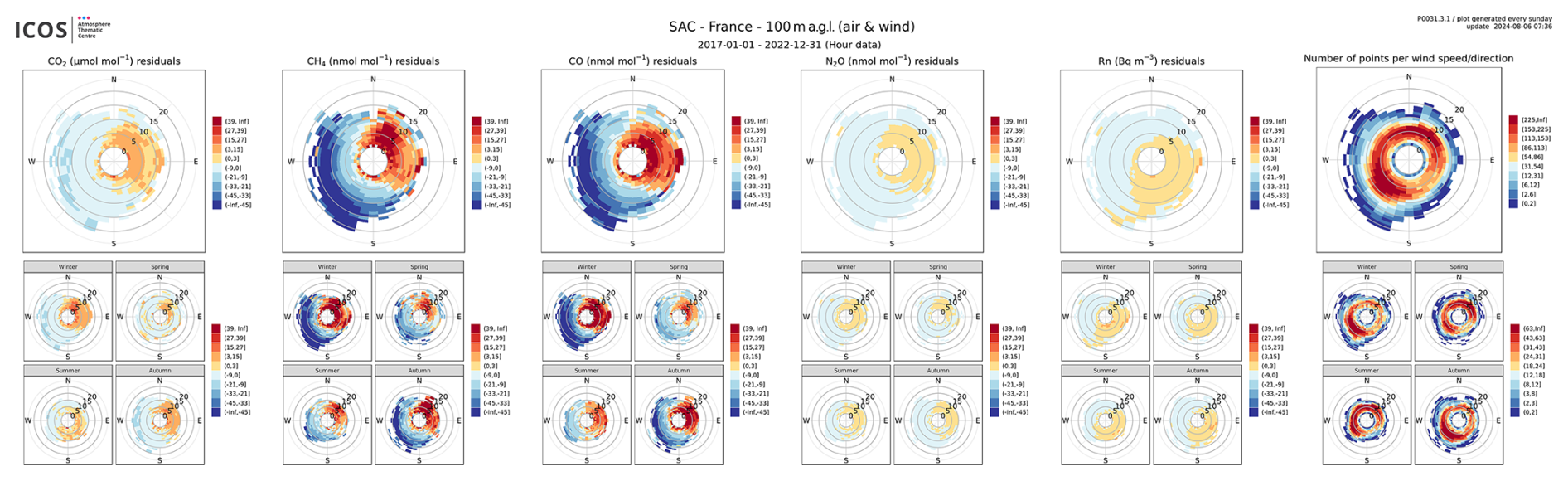
Figure 1 Mixing ratio and wind roses for CO₂, CH₄, CO, N₂O and ²²²Rn over the period 2017–2022. The residuals are calculated by subtracting the function fitted using the CCGCRV code, a digital filtering curve fitting program developed by Thoning et al. (1989) from the data (https://gml.noaa.gov/ccgg/mbl/crvfit/crvfit.html, last access: 14 November 2025). The top panels show the average residuals for the whole period while the lower panels are separated by season. The radial axis shows the wind speeds and for the GHG, the color scale shows the residual intensity while for the windrose, the color scale represents the wind frequency.

CO₂, CH₄, CO and N₂O are measured with cavity ring-down spectrometry analyzers from Picarro, Inc. In normal operation, one analyzer measures CO₂, CH₄ and CO (G2401 model) continuously at 100 m while two analyzers measure CO₂, CH₄, CO and N₂O (G2401 and G5310 models) sequentially at 15, 60 and 100 m spending 10 min per level. This allows us to use data average by 30 min to match the radon analyzer measurement frequency even for the N₂O data in the rest of the study. Air is dried using nafion membranes as in Welp et al. (2012), target gases are measured on a daily basis and calibration gases on a monthly basis. The measurement repeatability is estimated with the regular analysis of a target gas (Yver Kwok et al., 2015), which at Saclay can be rounded at about 0.03 ppm for CO₂, 0.1 ppb for CH₄, 0.3 ppb before 2019 then 0.03 ppb for CO (due to instrument change) and 0.05 ppb for N₂O. Systematic biases do no add uncertainty to the RTM as we are looking at mixing ratio differences. Using a nafion also reduces strongly any diurnal variations and thus any potential bias due to the water vapor influence. Thus, the uncertainties on the measurements are about 0.3 %, 0.3 %, 0.6 % then 0.06 % and 5 % of the diurnal cycle amplitude for CO₂, CH₄, CO and N₂O, respectively for the measurements at 100 m at Saclay. Radon is measured with a 1500 L ANSTO analyzer with a data every 30 min and its uncertainty is around 10 % with a sensitivity of approximatively 21 cpm (counts per minute) ${\mathrm{Bq}}^{-\mathrm{1}}{\mathrm{m}}^{-\mathrm{3}}$ as described in Whittlestone and Zahorowski (1998); Grossi et al. (2019); Chambers et al. (2022). For this study, we use the GHG and radon data measured at 100 m. To estimate how often this level is measuring above the nocturnal boundary height, we compared the nocturnal radon concentration at two heights, 15 and 100 m from February 2022 to June 2025 (we have no data at 15 m before). We calculated their correlation for all nights. We found that 80 % of the time, the two radon concentrations are well coupled and that the 100 m level stays below the boundary layer height making it suitable for our RTM study.

Figure 1 presents the mixing ratios and wind roses for CO₂, CH₄, CO and N₂O at 100 m over the 2017–2022 period. The main wind direction is south-west in winter and autumn while in spring, wind comes also often from the north-west. In summer, wind covers almost the whole quadrant except south and east. For any season, the elevated concentration of CO₂, CH₄, CO and N₂O are found in the north-west with the Paris area and further away the urbanised regions of Germany, Netherlands and Belgium.

2.2 The radon tracer method

In this study, we are focusing on the nocturnal accumulation RTM (e.g.: Levin et al., 1999; Schmidt et al., 2001; Biraud et al., 2000; Messager, 2007; Yver et al., 2009; Hammer and Levin, 2009; Lopez et al., 2012; Vogel et al., 2012; Belviso et al., 2013; Grossi et al., 2018; Belviso et al., 2020; Levin et al., 2021; Tong et al., 2023). The principle is based on the simplified assumption of a constant flux J_gas in a layer of height H during a nocturnal time window (8 to 10 h window) leading to the accumulation of the gas emitted. We can thus write the temporal variation of its concentration as:

$$\begin{array}{}\text{(1)}& {\displaystyle \frac{\mathrm{\Delta }{C}_{\text{gas}}}{\mathrm{\Delta }t}}={\displaystyle \frac{J_{\text{gas}}}{H}}\end{array}$$

with Δt being the time since the establishment of a stable boundary layer and ΔC_gas the temporal variation of the concentration over this period. The same can be written for radon with an additional radioactive decay term.

$$\begin{array}{}\text{(2)}& {\displaystyle \frac{\mathrm{\Delta }{C}_{\mathrm{Rn}}}{\mathrm{\Delta }t}}={\displaystyle \frac{J_{\mathrm{Rn}}}{H}}-{\mathit{\lambda }}_{\mathrm{Rn}}{C}_{\mathrm{Rn}}.\end{array}$$

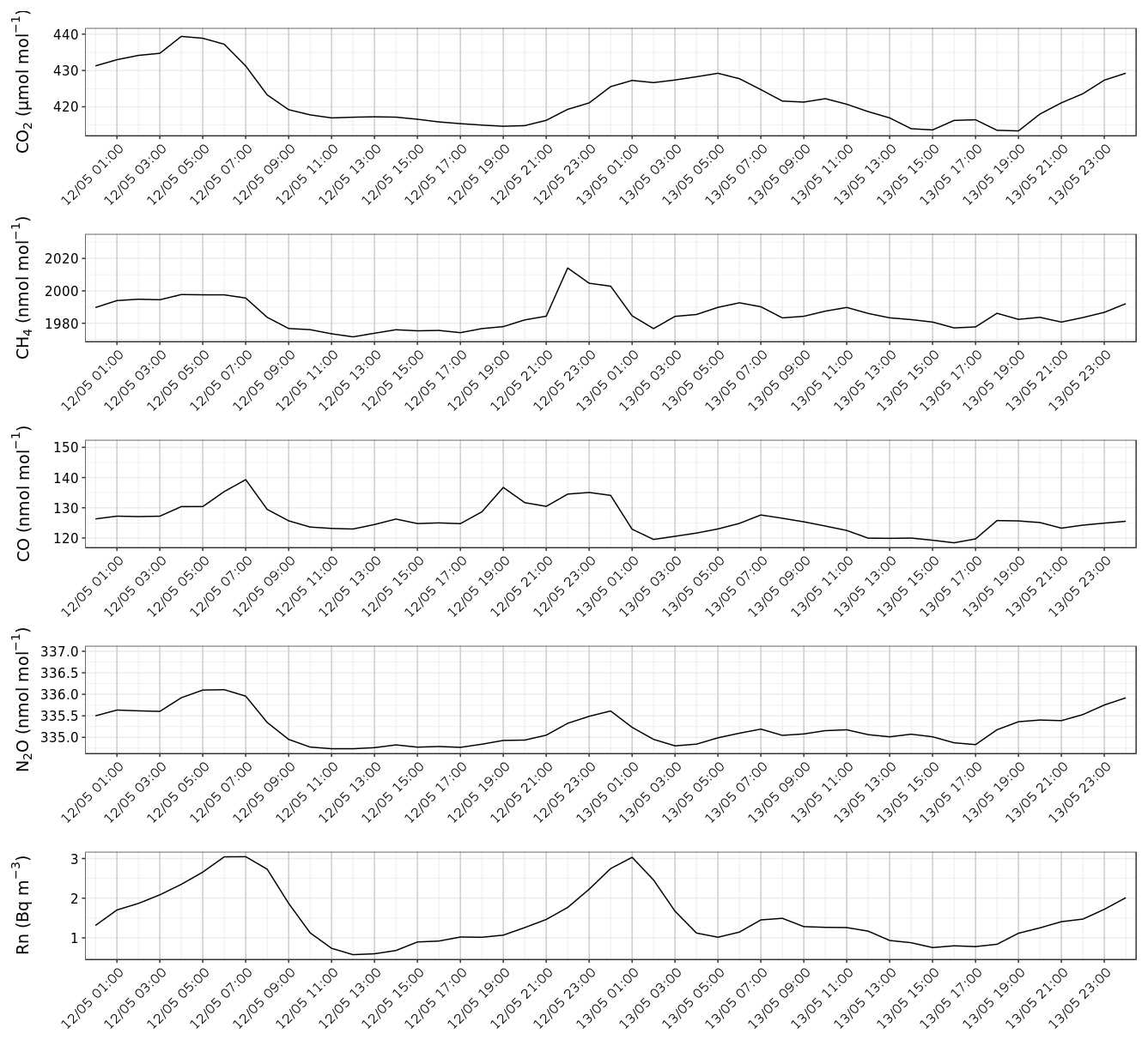
Figure 2 Two days in May 2021 showing CO₂, CH₄, CO, N₂O and ²²²Rn mixing ratios over time and their correlation. During the first night, R² equals 0.95, 0.91, 0.91 and 0.94 for CO₂, CH₄, CO and N₂O versus ²²²Rn, respectively. On the second night, R² equals 0.94 and 0.87 for CO₂ and N₂O versus ²²²Rn, respectively. CH₄ and CO are not correlated with ²²²Rn.

If we combine Eqs. (1) and (2) and we consider that for co-located measurement the height of the boundary layer is the same, we obtain:

$$\begin{array}{}\text{(3)}& J_{\text{gas}}=J_{\mathrm{Rn}}{\displaystyle \frac{\frac{\mathrm{\Delta }{C}_{\text{gas}}}{\mathrm{\Delta }t}}{\frac{\mathrm{\Delta }{C}_{\mathrm{Rn}}}{\mathrm{\Delta }t}}}{\left(\mathrm{1}+{\displaystyle \frac{{\mathit{\lambda }}_{\mathrm{Rn}}{C}_{\mathrm{Rn}}}{\frac{\mathrm{\Delta }{C}_{\mathrm{Rn}}}{\mathrm{\Delta }t}}}\right)}^{-\mathrm{1}}\end{array}$$

which, for ${\mathit{\lambda }}_{\mathrm{Rn}}{C}_{\mathrm{Rn}}\ll \frac{\mathrm{\Delta }{C}_{\mathrm{Rn}}}{\mathrm{\Delta }t}$ which is the case here, with a short-time period (one night) and a selection of events with enough radon build-up, simplifies to

$$\begin{array}{}\text{(4)}& J_{\text{gas}}=J_{\mathrm{Rn}}{\displaystyle \frac{\mathrm{\Delta }{C}_{\text{gas}}}{\mathrm{\Delta }{C}_{\mathrm{Rn}}}}\left(\mathrm{1}-{\displaystyle \frac{{\mathit{\lambda }}_{\mathrm{Rn}}{C}_{\mathrm{Rn}}}{\frac{\mathrm{\Delta }{C}_{\mathrm{Rn}}}{\mathrm{\Delta }t}}}\right).\end{array}$$

J_Rn is the ²²²Rn flux over the region of influence, $\frac{\mathrm{\Delta }{C}_{\text{gas}}}{\mathrm{\Delta }{C}_{\mathrm{Rn}}}$ is the slope of the linear regression between the observations of the gases. Both mixing height and net surface flux of the catchment area are averaged for the observation period, and $(\mathrm{1}-\frac{{\mathit{\lambda }}_{\mathrm{Rn}}{C}_{\mathrm{Rn}}}{\frac{\mathrm{\Delta }{C}_{\mathrm{Rn}}}{\mathrm{\Delta }t}})$ is the factor used to correct for ²²²Rn radioactive decay. In Levin et al. (2021), the whole effect of the decay, estimated to be less than 10 %, is neglected. Here, we apply the correction as defined in Schmidt et al. (2001). As observations for greenhouse gases are usually reported as mixing ratios, it is necessary to convert them into concentrations before applying the RTM. We use the molar volume at 288.15 K and 101 325 Pa to match the radon data treatment defined in Kikaj et al. (2025).

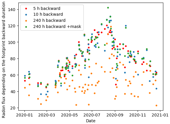
Figure 3 ²²²Rn flux calculated for the year 2020 for 5, 10 and 240 h long backtrajectories. For the 240 h long backtrajectory, a mask of about 300 km by 300 km representing the area of influence for the Saclay tower, was applied as well.

In this approach, the gas fluxes are considered similarly distributed in space and time, with no mixing of air from the free troposphere. The boundary layer height and the gas fluxes are assumed to remain constant during each nocturnal event. Figure 2 presents an example at Saclay, where the greenhouse gases and radon show the same behaviour and are thus good candidate to apply the RTM. During the first night, R² equals 0.95, 0.91, 0.91 and 0.94 for CO₂, CH₄, CO and N₂O versus ²²²Rn, respectively. On the second night, R² equals 0.94 and 0.87 for CO₂ and N₂O versus ²²²Rn, respectively. CH₄ and CO are not correlated with ²²²Rn.

When we combine the RTM with air particle backtrajectories, we do not assume a regular region of influence to the radon concentration, but we consider that the influence of each grid cell around the station depends on the residence time of the incoming air over that grid cell (footprint). Hence, the radon flux J_Rn is calculated weighting the radon flux of each gridcell by a sensitivity value (source-receptor matrix) obtained with the backtrajectory model (Seibert and Frank, 2004). In the case of the RTM, as we are interested by the accumulation over a short-period of time, the dispersion model should as well only run backwards for the same short period of time. More details on this approach are described in Grossi et al. (2018).

2.3 The RTM software

An interactive tool to apply the RTM to estimate GHG fluxes from ICOS atmospheric concentration measurement was developed (Yver, 2025). The code is written in Python and is hosted on the ICOS Carbon Portal (CP) JupyterLab. It thus takes advantage of the ICOS CP Python package to access ICOS site data and already calculated footprints.

By default, it uses the footprints already calculated by the Lagrangian model STILT as configured on the CP (available for all ICOS sites and more for at least 2018 to 2022 https://stilt.icos-cp.eu/viewer/, last access: 16 October 2025). The STILT footprints are available every 3 h and cover the region 33° S–73° N, 15° W–35° E with a resolution of $\mathrm{1}/\mathrm{12}$° by $\mathrm{1}/\mathrm{8}$°, approximately 10 km × 10 km. The STILT model is forced with the European Centre for Medium-Range Weather Forecast (ECMWF) Integrated Forecasting System (IFS) operational analysis. As these footprints are initially calculated for CO₂, no term for the radon radioactive decay has been added. By default, these footprints are going back in time for 10 d which is not suitable for our study. To correct this issue, we decided to apply a mask over the footprint representing the zone usually covered when going backward 5 to 10 h only. To do so, we calculated the mean wind speed over our period of study for the nights we had events. This average, 6 m s⁻¹, multiplied over the 8 h of our nocturnal window, gave us a radius of about 175 km. From this distance, we applied a rectangular mask centered on Saclay running from 50.28 to 47.15° N and −0.24 to 4.53° W. For the year 2020, we compared the radon flux calculated for different backward duration with the standard STILT run with and without applying our mask. On Fig. 3, we show the radon fluxes for 5, 10, 240 h with and without mask. We see, that with the mask the radon flux from the 10 d long backtrajectories is similar to the 5 and 10 h backtrajectories radon fluxes. Thus, we apply this mask for the rest of our study.

The radon exhalation maps used are the two new maps developed in the project 19ENV01 traceRadon (using new input data sets such as soil uranium content and physical soil properties and either the reanalysed moisture data from ERA5-Land (Muñoz Sabater, 2019) or GLDAS-Noah2.1 (Beaudoing and Rodell, 2020)) with a value per day and available from 2017 to 2024. Their resolution is 0.05° × 0.05° approximately 5.5 km latitude × 3.7 km longitude. All maps can be downloaded from the ICOS CP (Karstens and Levin, 2023, 2024).

Table 1 RTM runs for the sensitivity tests.

The radon exhalation maps and the footprints use different grids. Therefore, when combined, the radon exhalation maps are regridded to match the footprints.

The site to study can be chosen from the list available on the CP. The RTM can be applied to different species when data are available (CO₂, CH₄, N₂O and CO). Then, either it extracts the data from the CP Near Real Time hourly data or if the user has an access to the ICOS Atmosphere Thematic Center database with extraction rights for this site, data with a shorter timestep (minute data) can be extracted directly from the ICOS database and averaged on a 30 min window to match the highest resolution for the radon data.

By default, the code applies the RTM equation for the data between 21:00 to 06:00 UTC, which is a suitable window for central Europe where most of the ICOS stations are located, but this window can be modified to fit with other latitudes or longitudes for example to accommodate the shorter summer nights in northern Europe. The length of the window can be modified as well, for example to reproduce the tests from Levin et al. (2021). We apply an orthogonal distance regression using the SciPy.odr package.

No other criteria are applied initially but the correlation coefficient, the error in the linear regression, the number of data points and hours available for the calculation, the radon accumulation level and whether the radon rise stopped before 08:00 UTC are recorded so the data can be filtered in a second step.

3 Sensitivity study of the RTM

3.1 Run description

For the sensitivity study, we added the possibility of using Karstens et al. (2015) exhalation map and atmospheric radon activity measurements from other sources than what is available on the Carbon Portal. For the ANSTO detector, there is a measurement response time to consider, due to their design (a combined influence of their thoron delay volume, large measurement volume, and gross alpha counting approach, Griffiths et al., 2016). For an optimal utilisation of radon measurements, a standardized protocol for data processing is required allowing its stand-alone use in model comparisons or in combination with other gases as with the RTM. This is not done yet fully in any ICOS radon data treatment chain though the first step of temperature and pressure normalization is now applied. For this work, we have used a radon dataset derived from a standardized procedure, which is applicable to observations made by any similar (ANSTO made) radon monitoring system. The procedure to obtain the best estimate of atmospheric radon concentration (final product data) involves the traceability and the post-processing of radon data, which includes the crucial deconvolution routine (step to correct for the instrument response time) as well as correction for standard temperature and pressure (here using the International Standard Atmosphere, 288.15 K and 101 325 Pa). The details of the processing are available in Kikaj et al. (2025). The data that have been processed through this way are hereafter referred as standardized.

We also added the possibility to use footprints from another model. Each model grid has to be tailored to the footprint grid size. The FLEXPART-WRF model version 3.3.2 (Brioude et al., 2013) run at the Universitat Politècnica de Catalunya (UPC, Spain), is used here. This FLEXPART model uses WRF v4.2.1 output files as inputs for its back trajectory calculations. ECWMF ERA5 meteorological files were used as initial and lateral boundary conditions for WRF. This model was used with an output resolution of 0.05° in order to fit with the new ERA5-Land and GLDAS-Noah2.1 radon maps. The back trajectories were calculated for a 24 h window time, beginning at 00:00 UTC and assuming the 0–100 m layer as the footprint layer, which is suitable as 80 % of nights are indeed within this layer. For the Saclay site, the spatial domain used was 42.9–54.5° in latitude and −6–16.2° in longitude.

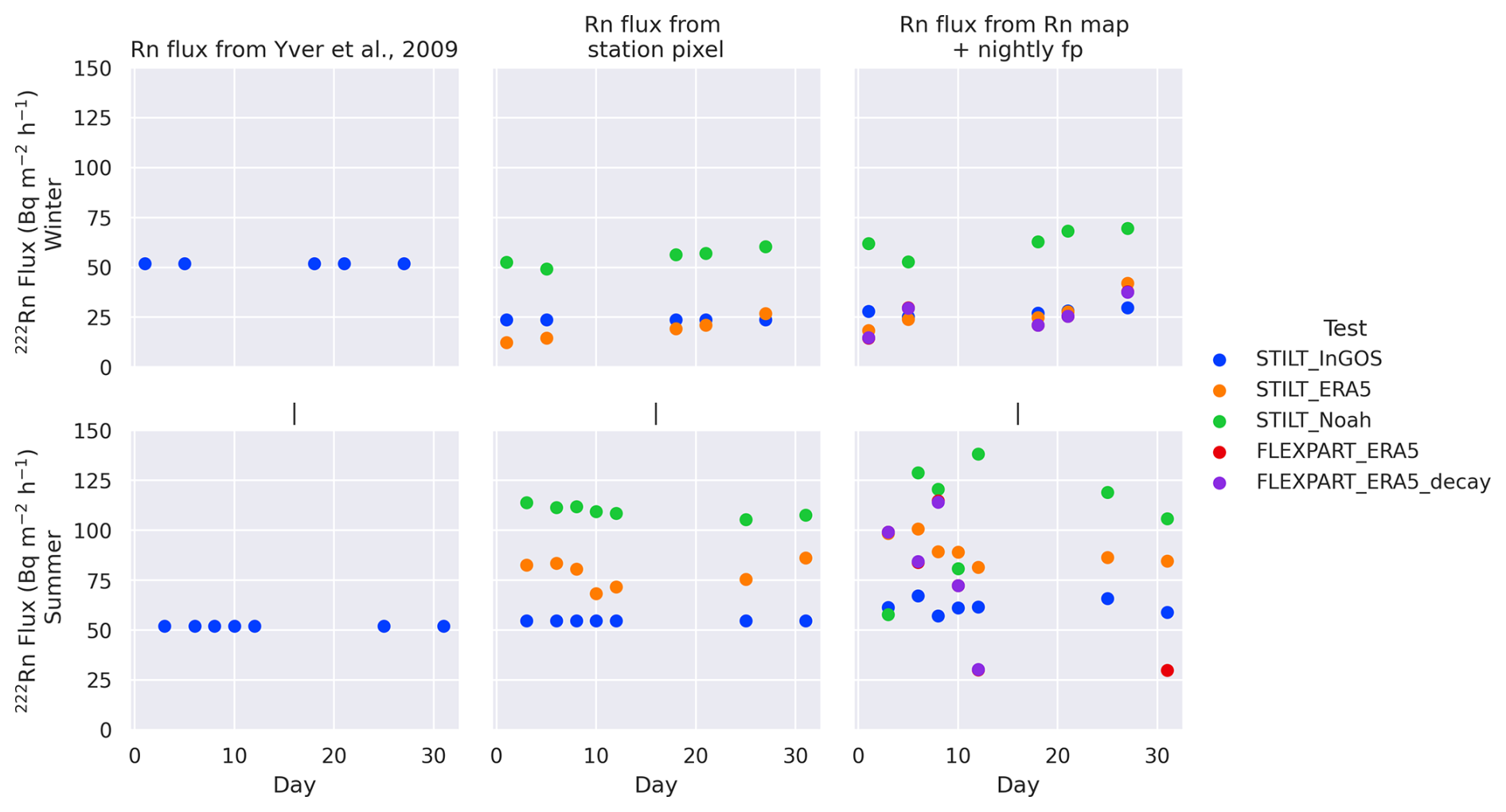
Figure 4 ²²²Rn flux in February (top) and August (bottom) 2019 for the sensitivity tests. On the left, the fixed flux established for Saclay (Yver et al., 2009) is displayed. In the middle, the fluxes are derived only from the station pixel of the different exhalation maps. On the right, the radon fluxes come from the combination of the exhalation maps and the nighttime footprint. The colored dots represent the fluxes for the different runs. For each panel, only the runs leading to different results are shown for clarity.

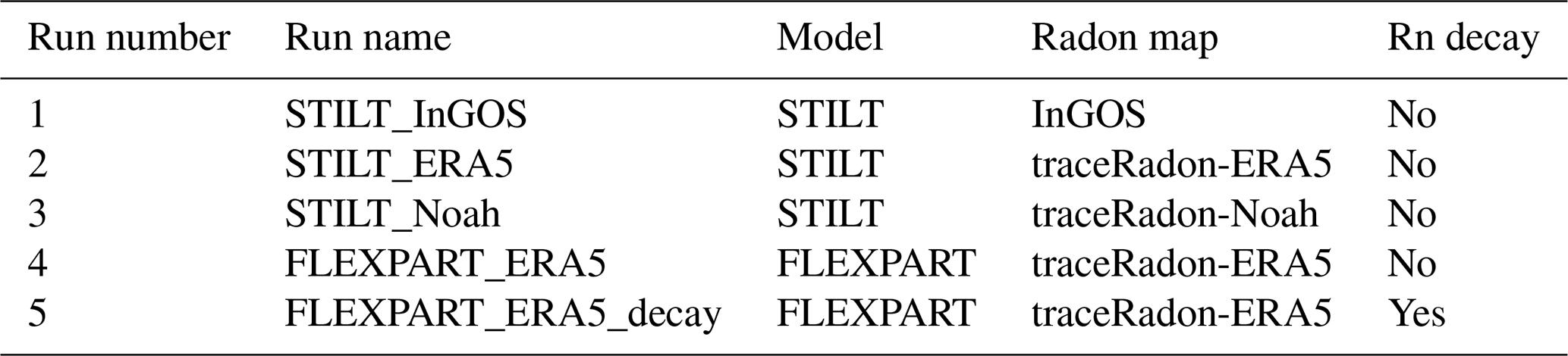
For the RTM runs (see Table 1), we used the three different radon exhalation maps available (called hereafter InGOS (climatology based on Karstens et al., 2015), traceRadon_ERA5, traceRadon_Noah), two models (CP-STILT, WRF-FLEXPART). By default, the two models do not compute the radon decay term. It is applied as a fixed term in the Eq. (3) as in Schmidt et al. (2001). For the last run, however, WRF-FLEXPART was modified to apply the Radon decay at each time step so the footprint already accounts for it. Not all combinations are tested but all runs can go in pairs, with only one change from one to the other. Two months were chosen: February 2019 and August 2019 to observe the seasonal influence and as months with a good data coverage for CH₄.

STILT_InGOS, STILT_ERA5 and STILT_Noah were carried out using footprints calculated with the same CP-STILT model configuration and the same atmospheric concentration radon and GHG data. In this case, the radon flux maps, InGOS, traceRadon-ERA5 and traceRadon_Noah were used to evaluate how radon fluxes calculated using different soil moisture reanalysis data could influence the final results. FLEXPART_ERA5 used the same configuration as STILT_ERA5, but with the FLEXPART-WRF based footprints which were calculated in the UPC cluster. Finally, FLEXPART_ERA5_decay was the same as FLEXPART_ERA5 with the radon decay directly included in the footprint calculations.

Radon fluxes were applied in different ways for each night during the 2 months:

1. constant radon flux value over the area of interest (52 $\mathrm{Bq}{\mathrm{m}}^{-\mathrm{2}}{\mathrm{h}}^{-\mathrm{1}}$, Yver et al., 2009);

2. radon flux values obtained with the available radon flux maps (InGOS, traceRadon_ERA5 and traceRadon_Noah) in the gridcell including the station. In the case of the InGOS map only one value per month was available while daily mean values are available for the two new traceRadon maps;

3. radon fluxes values obtained by coupling the previous radon flux maps with the atmospheric transport model (ATM) based footprints for the studied night.

Methane fluxes within this study were calculated for every day during the months of February 2019 and August 2019 using at least two hours (or four datapoints) in the linear correlation between radon and CH₄.

The linear fits calculated between nocturnal radon and CH₄ data at the Saclay stations were then filtered to retain only the meaningful events using the following criteria: R² > 0.6; error on the slope < 50 %; radon increase over the night > 1 Bq m⁻³. These values were chosen as a compromise between a high number of events and a very high correlation. They were used previously e.g. in Hammer and Levin (2009); Yver et al. (2009).

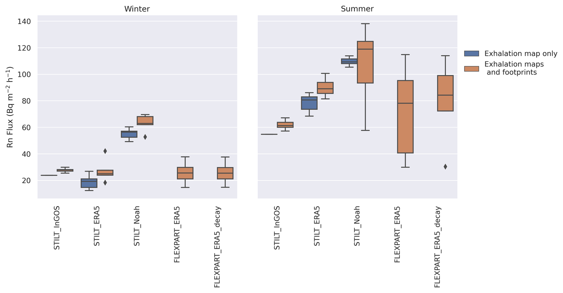
Figure 5 ²²²Rn mean flux in February (left) and August (right) 2019 for the sensitivity tests when using either only the exhalation rate maps or both the maps and the footprints.

3.2 RTM sensitivity evaluation

Figure 4 shows the daily radon flux for February 2019 at the top and August 2019 at the bottom for the different runs and three different fluxes. On the left, the fixed flux from Yver et al. (2009) is displayed. In the middle, the fluxes are derived only from the station pixel of the different exhalation maps. On the right, the radon fluxes come from the combination of the exhalation maps and the nighttime footprint. For each panel, only the runs leading to different results are shown, e.g. for the left panel, only STILT_InGOS is shown as model and ²²²Rn exhalation map are not used with the fixed flux from Yver et al. (2009). Results show that ²²²Rn fluxes in winter are generally lower than those in summer, as it was expected from the literature (Stranden et al., 1984). Indeed, in summer, the lower water content in the soil during this drier period leads to higher fluxes than in winter and spring, when the increased precipitations and the low temperatures lead to a reduced evaporation and an increased soil moisture that can prevent the radon to exhale. In the middle panels, daily radon fluxes based on GLDAS-Noah reanalysis (STILT_Noah) for this station pixel and period of time, display higher values than the ones calculated using ERA5-Land data (STILT_ERA5). Specifically daily fluxes vary between 12 and 27 $\mathrm{Bq}{\mathrm{m}}^{-\mathrm{2}}{\mathrm{h}}^{-\mathrm{1}}$ for STILT_ERA5 and in the range of 49 to 60 $\mathrm{Bq}{\mathrm{m}}^{-\mathrm{2}}{\mathrm{h}}^{-\mathrm{1}}$ for STILT_Noah, while STILT_InGOS is at 24 $\mathrm{Bq}{\mathrm{m}}^{-\mathrm{2}}{\mathrm{h}}^{-\mathrm{1}}$ in February 2019. In August 2019, they vary between 68 and 86 $\mathrm{Bq}{\mathrm{m}}^{-\mathrm{2}}{\mathrm{h}}^{-\mathrm{1}}$ for STILT_ERA5, between 105 and 112 $\mathrm{Bq}{\mathrm{m}}^{-\mathrm{2}}{\mathrm{h}}^{-\mathrm{1}}$ for STILT_Noah and STILT_InGOS is at 55 $\mathrm{Bq}{\mathrm{m}}^{-\mathrm{2}}{\mathrm{h}}^{-\mathrm{1}}$.

In the right panels, radon fluxes calculated using radon flux maps and ATM footprints show as expected a different variability, but the range is in the same order of magnitude. In February, the fluxes vary between 25 and 29 $\mathrm{Bq}{\mathrm{m}}^{-\mathrm{2}}{\mathrm{h}}^{-\mathrm{1}}$ for STILT_InGOS, 18 and 42 $\mathrm{Bq}{\mathrm{m}}^{-\mathrm{2}}{\mathrm{h}}^{-\mathrm{1}}$ for STILT_ERA5, 52 and 69 $\mathrm{Bq}{\mathrm{m}}^{-\mathrm{2}}{\mathrm{h}}^{-\mathrm{1}}$ for STILT_Noah, and 15 and 38 $\mathrm{Bq}{\mathrm{m}}^{-\mathrm{2}}{\mathrm{h}}^{-\mathrm{1}}$ for FLEXPART_ERA5. In August, the fluxes vary between 57 and 67 $\mathrm{Bq}{\mathrm{m}}^{-\mathrm{2}}{\mathrm{h}}^{-\mathrm{1}}$ for STILT_InGOS, 81 and 100 $\mathrm{Bq}{\mathrm{m}}^{-\mathrm{2}}{\mathrm{h}}^{-\mathrm{1}}$ for STILT_ERA5, 57 and 138 $\mathrm{Bq}{\mathrm{m}}^{-\mathrm{2}}{\mathrm{h}}^{-\mathrm{1}}$ for STILT_Noah and 30 and 115 $\mathrm{Bq}{\mathrm{m}}^{-\mathrm{2}}{\mathrm{h}}^{-\mathrm{1}}$ for FLEXPART_ERA5. We do not see significant differences between FLEXPART_ERA5 and FLEXPART_ERA5_decay showing that the approximation usually used for the radon decay is coherent with the model results and can be used without degrading the results when the ATM footprint does not include the decay.

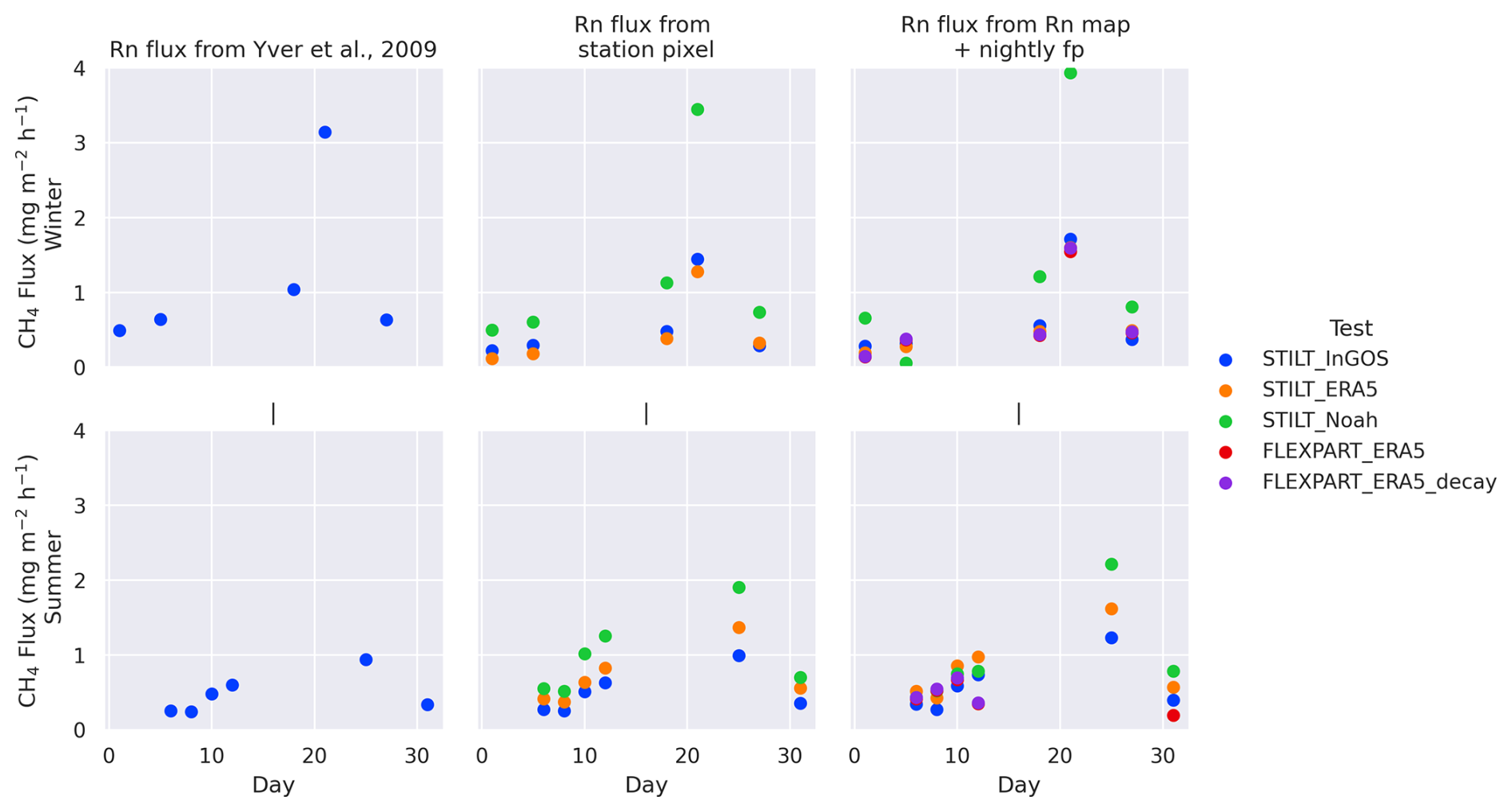
Figure 6 CH₄ flux in February (top) and August (bottom) 2019 for the sensitivity tests. On the left, the methane fluxes calculated using the radon fixed flux from Yver et al. (2009) is displayed. In the middle, the methane fluxes are derived only from the radon flux from the station pixel of the different exhalation maps. On the right, the methane fluxes are calculated with the radon fluxes coming from the combination of the exhalation maps and the nighttime footprint. The colored dots represent the fluxes for the different runs. For each panel, only the runs leading to different results are shown for clarity.

As shown in Fig. 5, in winter, the radon exhalation rate is driving the difference between the different tests. Between STILT_InGOS and STILT_Noah, there is a 97 % difference while between STILT_InGOS and the other runs, the difference is below 12 %. In summer, this difference is seen when using only the exhalation map pixel value but when using the footprint, the variability of all runs compared to STILT_ERA5 is between 5 % and 37 %. STILT_Noah still shows the higher difference but the FLEXPART model leads to difference almost as high using the lower radon exhalation rate as in STILT_ERA5.

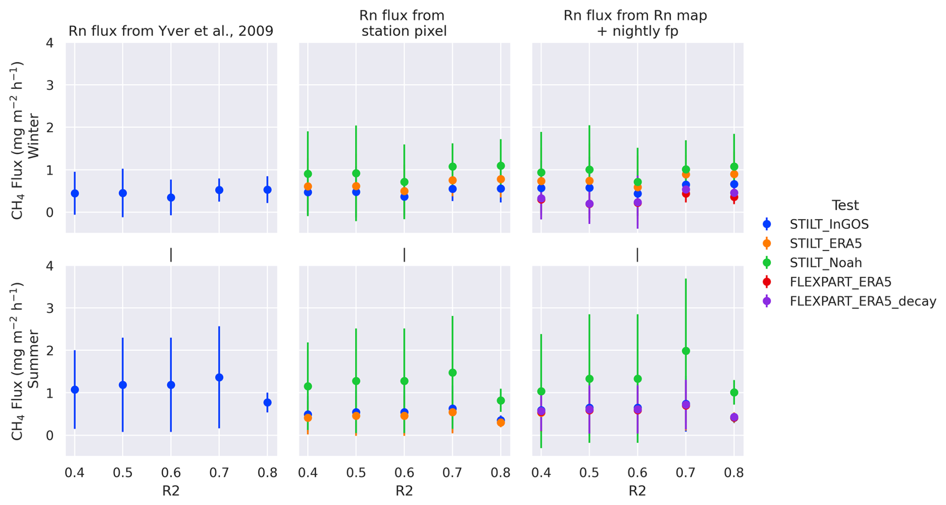
Figure 7 ²²²Rn averaged flux in February (top) and August (bottom) 2019 for the sensitivity tests in function of the R² cut-off. On the left, the fixed flux established for Saclay (Yver et al., 2009) is displayed. In the middle, the fluxes are derived only from the station pixel of the different exhalation maps. On the right, the radon fluxes come from the combination of the exhalation maps and the nighttime footprint. The colored dots represent the fluxes for the different runs. The vertical error bars show the standard deviation. For each panel, only the runs leading to different results are shown for clarity.

As can be expected, the variability on the radon fluxes is seen as well on the CH₄ fluxes (see Fig. 6), reflecting that the day to day variation is due not only to the emission variations but also to the the different areas that are sampled. We observe values around 0.5 $\mathrm{mg}{\mathrm{CH}}_{\mathrm{4}}{\mathrm{m}}^{-\mathrm{2}}{\mathrm{h}}^{-\mathrm{1}}$ in winter and summer with more variability in summer. On 21 February, the values are particularly high compared to the other winter values, peaking at more than 3 $\mathrm{mg}{\mathrm{CH}}_{\mathrm{4}}{\mathrm{m}}^{-\mathrm{2}}{\mathrm{h}}^{-\mathrm{1}}$ when using STILT_Noah. On that day, the correlation is strong with an R² at 0.76 and high concentration of CH₄, CO₂ and CO while the radon accumulation is small, just above the threshold. There is no rain but a wind direction change just at the beginning of the period form south-west to south-east that may have brought polluted local air masses.

To check the effect of the chosen R² cut-off value, we have calculated the average radon flux for each run depending on which R² cut-off we chose, from 0.4 to 0.8. This is shown on Fig. 7. Depending on the R² cut-off value, the average flux is varying, however, considering the standard deviation, the variations are not significant and confirm that a cut-off value of 0.6 is a good compromise between high correlation and number of events selected.

This study highlights the impact of the radon exhalation rate. The transport models used here have less impact. Moreover, using a simplified decay term compared to have this term included in the model leads to insignificant differences.

4 Eight years of CO₂, CH₄, CO and N₂O flux estimates

Following the findings from the sensitivity study, for Saclay, we used standardized radon data, radon exhalation rate coming from the map using GLDAS-Noahv2.1 combined with the STILT footprint of each night (an aggregate of 3 footprints from 21:00, 00:00 and 03:00 UTC). We combined them with CO₂, CH₄, CO and N₂O data from the ICOS database at a 30 min interval between 21:00 and 06:00 UTC. We chose to use the map using GLDAS-Noahv2.1 as Karstens and Levin (2024) showed that for Saclay, STILT_Noah using the GLDAS-Noahv2.1 moisture parametrization and STILT model was exhibiting the smallest differences compared to measured data.

Figure 8 ²²²Rn flux from 2017 to 2024 for CO₂ selected nights using STILT_Noah.

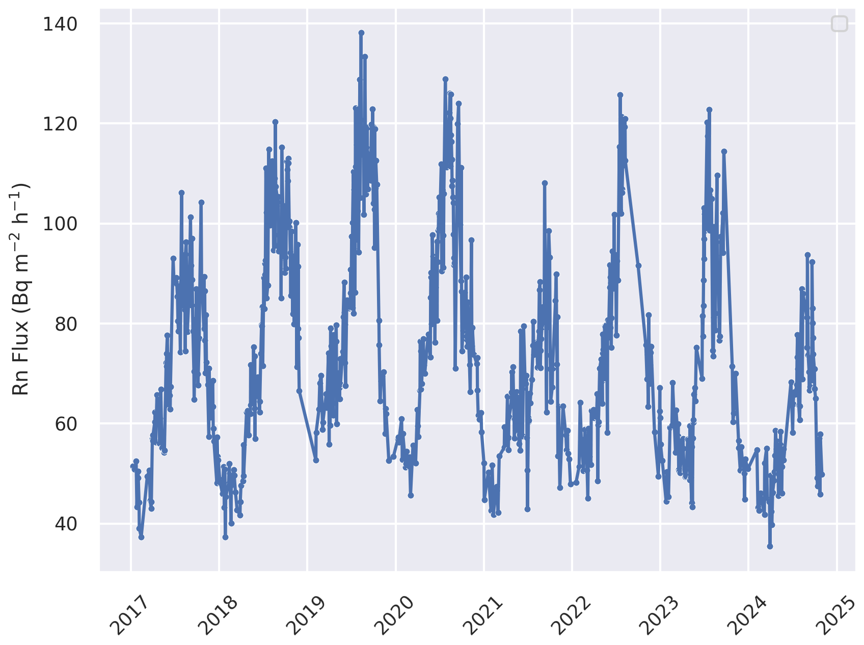
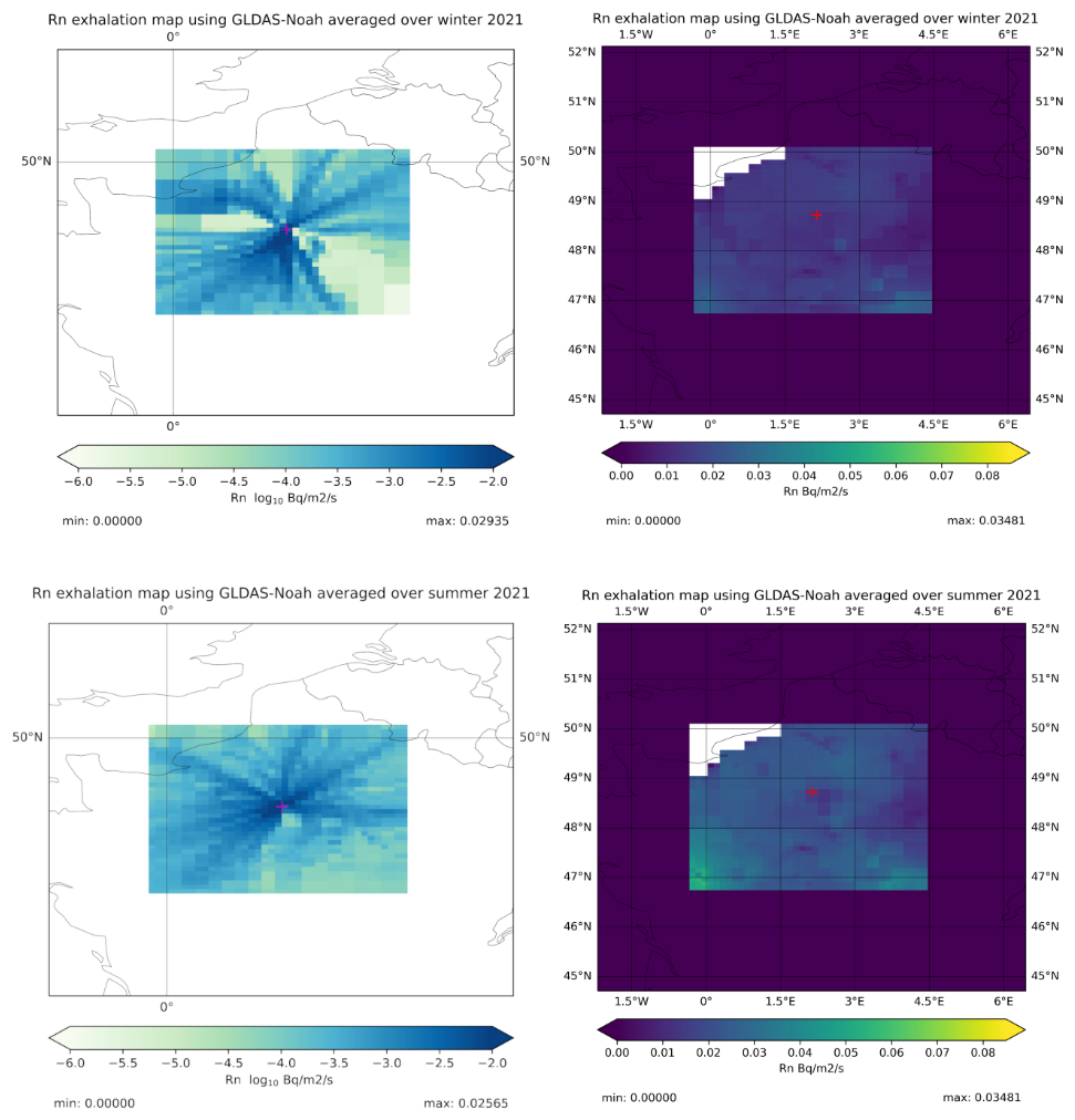
Figure 9 Saclay STILT footprint averaged over the RTM selected days for CH₄ in winter and summer 2021 along with the traceRadon_Noah exhalation rate map for the same periods. Winter is on top and summer on the bottom. On the left panels, the footprints zoomed around SAC are shown. The color scale represents the sensitivity of each pixel to the emissions reaching SAC. The exhalation rate maps are shown on the right panels. A mask representing the Saclay influence area is applied to the maps.

4.1 Radon fluxes

Figure 8 shows the radon exhalation rate from 2017 to 2024 from the exhalation map combined with the night footprints as in STILT_Noah. Using the exhalation map allows to follow the seasonal pattern of the radon exhalation rate driven by humidity (Stranden et al., 1984) with a summer maximum and winter minimum. The average winter and summer footprint calculated using the RTM selected nights for 2021 are shown in Fig. 9 together with the radon exhalation averaged over the same period. We show only the footprints and radon exhalation rate within our mask. We clearly see the increased radon exhalation rate in summer compared to winter in the right panels. The difference in the footprint is less marked but in winter a narrow west sector and the south-east sector do not influence the station while in summer, the station is influenced from all sectors with a reduced influence in the south. Over the 8 years, the average radon flux rate estimated from the footprint analysis applied to the GLDAS-Noah map reaches 75 $\mathrm{Bq}{\mathrm{m}}^{-\mathrm{2}}{\mathrm{h}}^{-\mathrm{1}}$ which is 44 % higher than the literature value that has been used previously. The minimum is 35 $\mathrm{Bq}{\mathrm{m}}^{-\mathrm{2}}{\mathrm{h}}^{-\mathrm{1}}$ and the maximum 138 $\mathrm{Bq}{\mathrm{m}}^{-\mathrm{2}}{\mathrm{h}}^{-\mathrm{1}}$ leading to a larger amplitude than previously applied at Saclay (25 % Yver et al., 2009). We also observe an annual variability with the lowest values in 2017 and the highest in 2019 (see Fig. 8). In 2017, 2021 and in 2024, the amplitude is smaller with less high values in summer than the other years. This is linked with the moisture reproduced by the GLDAS-Noah model, as can be seen in Fig. 10 for 2017 and 2021 where these years show higher moisture content in summer than during the other years. 2024 has also known an excess of precipitation leading to increased soil moisture as well (WMO, 2024).

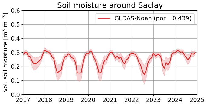
Figure 10 Soil moisture content for the pixel containing SAC as modeled in GLDAS-Noahv2.1 from 2017 to 2025 with a porosity (noted por on the figure) of 0.439.

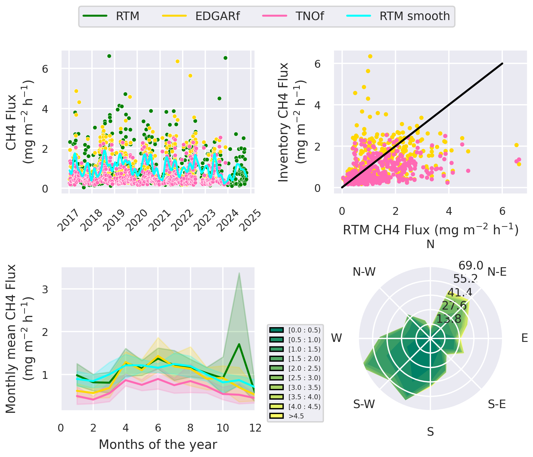
Figure 11 The CH₄ fluxes (RTM), calculated using the STILT_Noah configuration were compared with the smoothed fluxes (RTM smooth), the combined EDGAR and TNO inventories using the same footprints for the period 2017–2024 (EDGARf and TNOf, respectively). The top left panel shows all the selected nocturnal fluxes (colored dots), the top right panel shows the correlation between the RTM fluxes and the inventory estimates. The bottom left plot shows the seasonal cycles of the fluxes while the bottom right plot shows the flux repartition over the windrose with the flux intensity as the color scale and its frequency on the axial axe.

4.2 Bottom-up emissions

We use two different bottom-up inventories for comparison to the RTM derived GHG fluxes. The first one is EDGARv2024 (Crippa et al., 2024). These are gridded annual anthropogenic fluxes with a 0.1° resolution over the world for CO₂, CH₄ and N₂O covering 2017 until the end of 2023. For CO₂, CH₄ and CO, we use the Netherlands Organisation for Applied Scientific Research (TNO) inventory (Kuenen et al., 2014; Super et al., 2020) which provides anthropogenic fluxes with a 6 km resolution over Europe. Monthly, weekly and daily profiles can be added to the TNO emission map. For this work, we only apply the monthly profile to the TNO inventory to reflect the seasonal changes covering 2017 until the end of 2023.

For biogenic CO₂ fluxes, we compare our results to simulations using the WRF-VPRM model with a 5 km resolution around the Ile-de-France area (Lian et al., 2019) covering 2017 to the end of 2022. WRF-VPRM winds were forced by the hourly reanalysis fields from the fifth generation of meteorological analysis of the ECMWF at 0.75° × 0.75° resolution, respectively (ECMWF ERA5, Hersbach et al., 2020). The VPRM model is forced by meteorological fields simulated by WRF and online-coupled to the atmospheric transport. It uses vegetation indices derived from the 8d MODIS Surface Reflectance Product (MOD09A1) and four parameters optimized using data from the Integrated EU project “CarboEurope-IP” (https://www.copernicus.eu/en/carbo-europe-ip, last access: 16 October 2025). VPRM uses a land cover derived from the 1 km global Synergetic Land Cover Product (SYNMAP; Jung et al., 2006) reclassified into eight different vegetation classes (Ahmadov et al., 2007, 2009).

EDGAR, TNO and VPRM fluxes have been combined with the footprint of each selected event to calculate the fluxes comparable to the fluxes estimated with the RTM. In the rest of the text, we call these combinations EDGARf, TNOf and VPRMf.

4.3 Uncertainties

To assess the validity of the fluxes deduced from the RTM and provided by inventories, we need to estimate their uncertainties. Here, the uncertainty of one RTM-based GHG flux estimate is the combination of the measurement uncertainty as described in Sect. 2.1, the linear regression uncertainty on the slope and the radon flux uncertainty. To calculate the total uncertainty, we propagate the errors with a standard summation in quadrature. The errors on the slopes and on the greenhouse gas measurements are standard deviation of the estimated parameters. The uncertainty on the model comes from Karstens et al. (2015), and is itself calculated as the propagation of errors from different sources. They stem mostly from the differences between the model and observed values. The error for our detector comes as described in more details in Grossi et al. (2020), as the combination of a calibration source uncertainty of 4 %, a coefficient of variability of valid monthly calibrations of 2 %–6 %, and accounting uncertainty of around 2 % for radon concentrations above 1 Bq m⁻³.

For the four species, the uncertainties on the linear regression is in average 14 %, which combined with the measurement uncertainties yields a maximum uncertainty of 15 % on the slope. The full uncertainty depends critically on the uncertainty in the modelled radon fluxes. Based on the underlying radon flux model and the assumed uncertainties in the input parameters, Karstens et al. (2015) estimated the uncertainty of modelled fluxes for individual pixels to about 50 % and to approximately 30 % when averaged over a larger area like in this application. Additionally, the radon flux maps show large differences depending on the soil moisture reanalysis that were used in the model (see Fig. 3 middle panel). Calibration of the radon flux map in the footprint region with long term measurements at the station could help to reduce this systematic uncertainty, while retaining information on temporal and spatial variability (Levin et al., 2021). We estimate here the RTM maximum total uncertainty at 35 %. It is worth to note that the systematic errors or biases that are seen here are of less impact when studying the long term trend of emissions. In our study, we estimate 8 years of data and thus can begin to draw conclusions about potential trends.

EDGAR's uncertainties are discussed in details in Solazzo et al. (2021). CO₂ uncertainties are low, estimated at 7 % for the energy sector which represents 96 % of the global emissions. For CH₄ and N₂, the uncertainties are much higher, reaching for example around 50 % in the waste domain for CH₄ and more than 300 % for N₂O in the agricultural or waste domains.

TNO's uncertainties are discussed in Super et al. (2020) but only for CO₂ and CO. For the domain, a European region centred over the Netherlands and Germany, the uncertainties for the total emissions are 1 % for CO₂ and 6 % for CO. The largest contributor of uncertainties for CO₂ is the public power category while it is the stationary combustion for CO. The uncertainty increases up to 40 % for CO₂ and 70 % for CO if looking at specific grid cells.

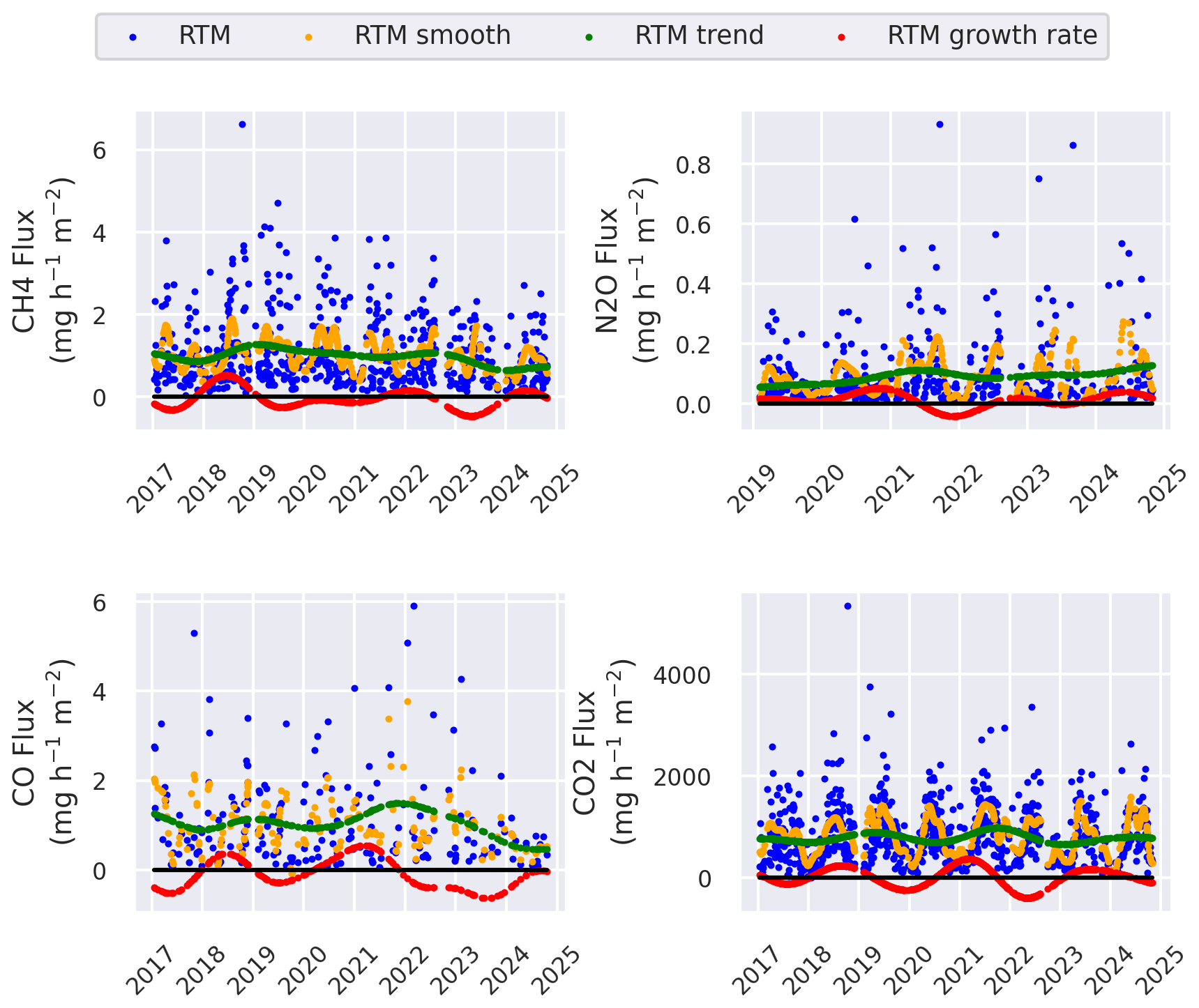
Figure 12 RTM calculated fluxes along with their smoothed values, trend and growth rates estimated using the CCGCRV code. Each panel shows a different species.

4.4 CH₄ fluxes

Figure 11 shows the fluxes of CH₄ calculated using the STILT_Noah configuration with the footprints. The figure also includes the bottom-up flux estimate for each footprint using EDGAR and TNO. The averages over 2017–2024 are shown in Table 2. On Fig. 12, in the top left panel, the RTM fluxes with the smoothed fluxes, their trend, and growth rate are shown.

Table 2 GHG fluxes ($\mathrm{mg}{\mathrm{m}}^{-\mathrm{2}}{\mathrm{h}}^{-\mathrm{1}}$) averaged over the measurement period (2017–2024 or 2019–2024) for the RTM estimates fluxes using the STILT_Noah configuration, for EDGARf, TNOf and VPRMf estimates. The second value represents the standard deviation over the whole period.

First, the RTM fluxes, EDGARf and TNOf are in a relatively good agreement showing a similar variability visible in the top left panel. No clear trend is observed although we do observe a small seasonal cycle, with lower emission in winter and higher in summer. January and February are usually showing lower emissions than the other months and fewer events in total. As EDGARf variability only comes from the footprints (annual inventory), this would be indicative of a sector with low emissions or no correlation sampled more often during these months. This can be due to the CEA research center boiler room located very close to the station, which signature can be seen when the wind is coming from the north-northeast. In case of the airmass coming over the boiler, the radon and methane would not present a correlation anymore. In January 2019, there was a lack of radon data for half of the month (16 d without data) as only one event was found in January. However, in December 2018, there was no lack of data but no event found. For this month, the correlation was too low for 19 d and for the other non-selected days, it was either the radon increase or the number of available hours that were too low (below 1 Bq m⁻³ for the radon increase or less than 2 h of duration for the available data). In November 2021, there is no lack of data but only one event selected. Here, as well, the correlation was too low for 19 d. This seems mostly due to relatively strong winds, leading to a relatively flat radon concentration over night and thus no correlation.

The RTM gives an average of 1.10 ± 0.89 $\mathrm{mg}{\mathrm{CH}}_{\mathrm{4}}{\mathrm{m}}^{-\mathrm{2}}{\mathrm{h}}^{-\mathrm{1}}$ which compares well with the EDGARf average of 0.99 ± 0.86 $\mathrm{mg}{\mathrm{CH}}_{\mathrm{4}}{\mathrm{m}}^{-\mathrm{2}}{\mathrm{h}}^{-\mathrm{1}}$ within the range of uncertainties. The TNOf value is a third smaller than the RTM estimate with 0.68 ± 0.50 $\mathrm{mg}{\mathrm{CH}}_{\mathrm{4}}{\mathrm{m}}^{-\mathrm{2}}{\mathrm{h}}^{-\mathrm{1}}$. This is obvious in Fig. 11 right top panel where we can see that most of TNOf emissions are lower than the RTM. For EDGARf, in the lower range, the agreement is better but for the higher values, the RTM is systematically above EDGARf. As expected, the bottom right plot shows the highest emissions coming from the north-east, hence from the Paris area. Both EDGAR and TNO have agriculture and waste as the first most important sectors for Saclay average footprint, accounting for almost 80 % of all the emissions with about the same share for the two sectors. The difference between the two inventories seems then to be in the total emissions and not in their sectorisation in this footprint.

Using the RTM, Levin et al. (2021) calculated an estimate for the Heidelberg region between 2015 and 2020 which reached an average of 0.8 $\mathrm{mg}{\mathrm{CH}}_{\mathrm{4}}{\mathrm{m}}^{-\mathrm{2}}{\mathrm{h}}^{-\mathrm{1}}$ while in Cabauw between 2016 and 2018 (Tong et al., 2023), the estimate reached 1.4 $\mathrm{mg}{\mathrm{CH}}_{\mathrm{4}}{\mathrm{m}}^{-\mathrm{2}}{\mathrm{h}}^{-\mathrm{1}}$ with the RTM or 1.48 ${\mathrm{CH}}_{\mathrm{4}}{\mathrm{m}}^{-\mathrm{2}}{\mathrm{h}}^{-\mathrm{1}}$ with the vertical gradient method highlighting the importance of dairy farming in this region. At Gif-sur-Yvette, neighbouring Saclay, values of 0.8 $\mathrm{mg}{\mathrm{CH}}_{\mathrm{4}}{\mathrm{m}}^{-\mathrm{2}}{\mathrm{h}}^{-\mathrm{1}}$ were found for the period 2002–2007 using the RTM and the boundary layer height (Messager, 2007).

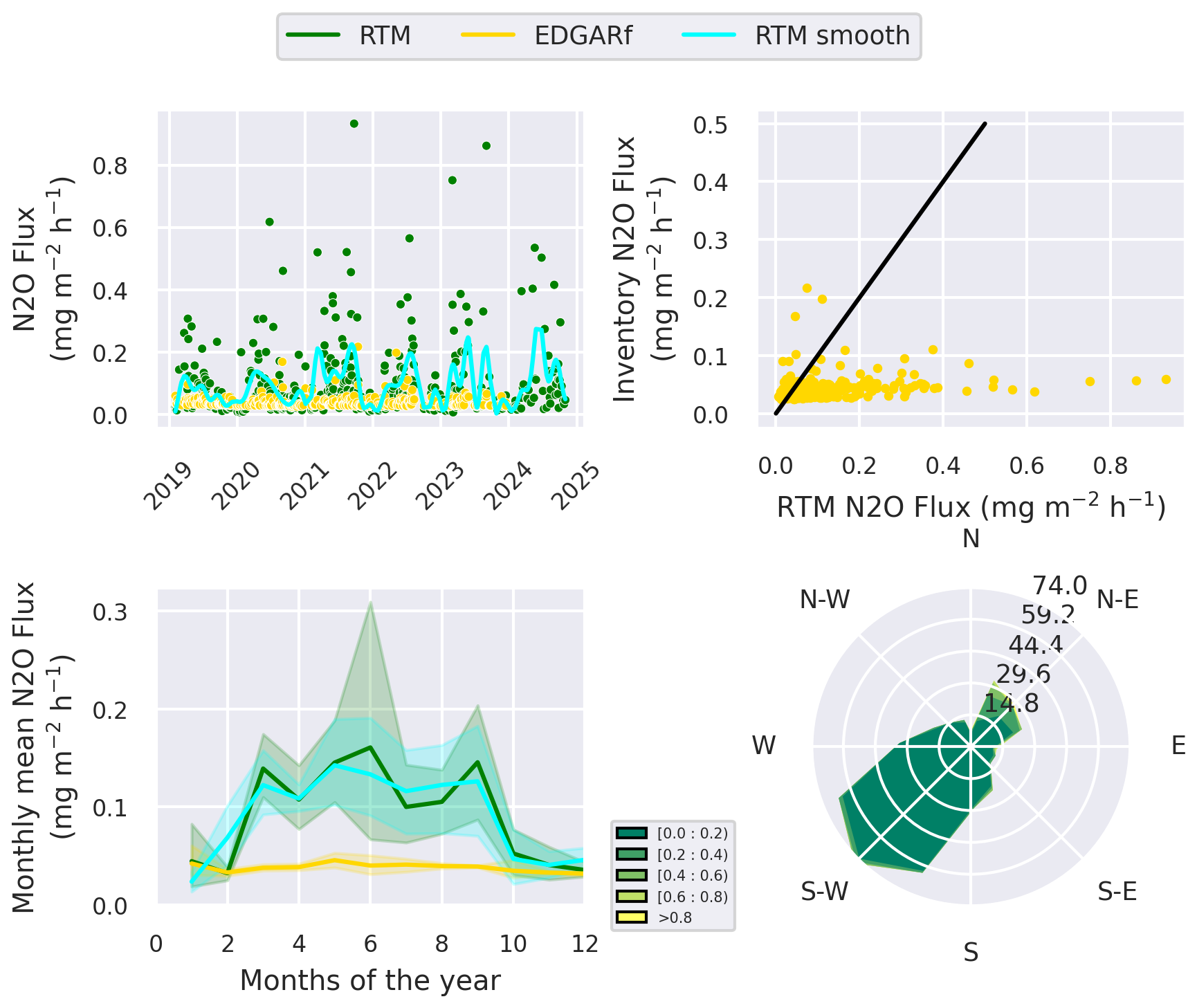
Figure 13 The N₂O fluxes (RTM), calculated using the STILT_Noah configuration were compared with the smoothed fluxes (RTM smooth), the combined EDGAR inventory using the same footprints for the period 2019–2024 (EDGARf). The top left panel shows all the selected nocturnal fluxes (colored dots), the top right panel shows the correlation between the RTM fluxes and the inventory estimates. The bottom left plot shows the seasonal cycles of the fluxes while the bottom right plot shows the flux repartition over the windrose with the flux intensity as the color scale and its frequency on the axial axe.

4.5 N₂O fluxes

The fluxes of N₂O calculated using the STILT_Noah configuration with the footprints are shown in Fig. 13. As for CH₄, the smoothed data, trend and growth rate are shown on Fig. 12, albeit on the top right panel. As shown in the left panels, the RTM fluxes show a seasonal variability with a maximum around spring and summer while the EDGARf fluxes do not, reflecting the fact that it is a yearly estimate and that the seasonality is not driven by the variability of air mass origins. No trend is observed. N₂O RTM fluxes for 2019 and 2020 show the highest values in spring followed by a decrease over the rest of the year. For the other years, the fluxes show spring high values as well but also in summer with higher values than the previous years in average that could reflect a change in the agricultural practices. EDGARf shows much lower values than the RTM fluxes in average: 0.038 $\mathrm{mg}{\mathrm{N}}_{\mathrm{2}}\mathrm{O}{\mathrm{m}}^{-\mathrm{2}}{\mathrm{h}}^{-\mathrm{1}}$ versus 0.094 $\mathrm{mg}{\mathrm{N}}_{\mathrm{2}}\mathrm{O}{\mathrm{m}}^{-\mathrm{2}}{\mathrm{h}}^{-\mathrm{1}}$, being close to the lower values estimated with the RTM. Indeed, when calculating the median, the difference decreases with 0.052 $\mathrm{mg}{\mathrm{N}}_{\mathrm{2}}\mathrm{O}{\mathrm{m}}^{-\mathrm{2}}{\mathrm{h}}^{-\mathrm{1}}$ versus 0.031 $\mathrm{mg}{\mathrm{N}}_{\mathrm{2}}\mathrm{O}{\mathrm{m}}^{-\mathrm{2}}{\mathrm{h}}^{-\mathrm{1}}$ for RTM and EDGARf, respectively. The top right panel shows indeed a better correlation between RTM and inventory values for the lower RTM values (< 0.1 $\mathrm{mg}{\mathrm{N}}_{\mathrm{2}}\mathrm{O}{\mathrm{m}}^{-\mathrm{2}}{\mathrm{h}}^{-\mathrm{1}}$) but systematic lower values of the inventory compared to the RTM values for the higher RTM values (> 0.1 $\mathrm{mg}{\mathrm{N}}_{\mathrm{2}}\mathrm{O}{\mathrm{m}}^{-\mathrm{2}}{\mathrm{h}}^{-\mathrm{1}}$). Agricultural soils are the main sector in EDGAR, accounting for more than 50 % of the total but the spikes during fertilization episodes are not reported as it is a yearly estimate. The bottom right panel highlights this pattern, with most of the events located in the south-west where agriculture is more predominant than in the north-east where Paris and its suburban areas lie.

N₂O fluxes were estimated at Cabauw as well (Tong et al., 2023) with an estimate of 0.046 $\mathrm{mg}{\mathrm{N}}_{\mathrm{2}}\mathrm{O}{\mathrm{m}}^{-\mathrm{2}}{\mathrm{h}}^{-\mathrm{1}}$ with RTM and 0.068 $\mathrm{mg}{\mathrm{N}}_{\mathrm{2}}\mathrm{O}{\mathrm{m}}^{-\mathrm{2}}{\mathrm{h}}^{-\mathrm{1}}$ with the vertical gradient method. At Gif-sur-Yvette, values of 0.068 $\mathrm{mg}{\mathrm{N}}_{\mathrm{2}}\mathrm{O}{\mathrm{m}}^{-\mathrm{2}}{\mathrm{h}}^{-\mathrm{1}}$ were reported for the period 2002–2007 by Messager (2007) but within the range of 0.039 to 0.058 $\mathrm{mg}{\mathrm{N}}_{\mathrm{2}}\mathrm{O}{\mathrm{m}}^{-\mathrm{2}}{\mathrm{h}}^{-\mathrm{1}}$ over the period 2002–2011 in Lopez et al. (2012). These values are of the same order of magnitude as the values found in this study. In studies measuring fluxes directly in agricultural soils using accumulation chambers within the Ile-de-France region over several years (Colnenne-David et al., 2021; Garnier et al., 2024), maximum values of 1.4 $\mathrm{mg}{\mathrm{N}}_{\mathrm{2}}\mathrm{O}{\mathrm{m}}^{-\mathrm{2}}{\mathrm{h}}^{-\mathrm{1}}$ and 2.3 $\mathrm{mg}{\mathrm{N}}_{\mathrm{2}}\mathrm{O}{\mathrm{m}}^{-\mathrm{2}}{\mathrm{h}}^{-\mathrm{1}}$ were found and in general high values were distributed over spring and summer months. The average values reached 0.09 and 0.05 $\mathrm{mg}{\mathrm{N}}_{\mathrm{2}}\mathrm{O}{\mathrm{m}}^{-\mathrm{2}}{\mathrm{h}}^{-\mathrm{1}}$, respectively. Garnier et al. (2024) also studied the factors influencing the N₂O releases and found that rainfall (hence soil moisture) had the largest influence over N₂O emissions, followed by daily maximum temperature.

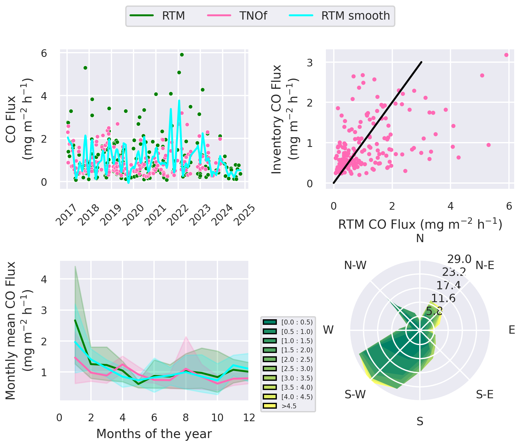
Figure 14 The CO fluxes (RTM), calculated using the STILT_Noah configuration were compared with the smoothed fluxes (RTM smooth), the combined TNO inventory using the same footprints for the period 2017–2024 (TNOf). The top left panel shows all the selected nocturnal fluxes (colored dots), the top right panel shows the correlation between the RTM fluxes and the inventory estimates. The bottom left plot shows the seasonal cycles of the fluxes while the bottom right plot shows the flux repartition over the windrose with the flux intensity as the color scale and its frequency on the axial axe.

4.6 CO fluxes

Figure 14 shows the fluxes of CO calculated using the STILT_Noah configuration with the footprints. As for CH₄, the smoothed data, trend and growth rate are shown on Fig. 12, albeit on the bottom left panel. CO RTM and TNOf fluxes do not show a clear seasonal cycle though higher fluxes are found in January. A slight decreasing trend is visible over the period especially since 2022. The RTM fluxes reach an average of 1.01 $\mathrm{mg}\mathrm{C}\mathrm{0}{\mathrm{m}}^{-\mathrm{2}}{\mathrm{h}}^{-\mathrm{1}}$. This is consistent with the TNOf values for the same area. In the top right panel , we see that values above 4 $\mathrm{mg}\mathrm{C}\mathrm{0}{\mathrm{m}}^{-\mathrm{2}}{\mathrm{h}}^{-\mathrm{1}}$ are systematically underestimated by the inventory, but the most part, they fall around the 1:1 line. For CO, more than 50 % of the emissions come from the residential sector (other stationary combustion sources), then 20 % from the road transport and 10 % from the industry. Most of the fluxes are located in the south-west quadrant, maybe indicative of a local source coming from the development of the university campus close to the site. Messager (2007) found an average value of 1.46 $\mathrm{mg}\mathrm{C}\mathrm{0}{\mathrm{m}}^{-\mathrm{2}}{\mathrm{h}}^{-\mathrm{1}}$ for Europe using measurement from Mace Head, Ireland over the period 1996–2006 with a tendency to decrease over time.

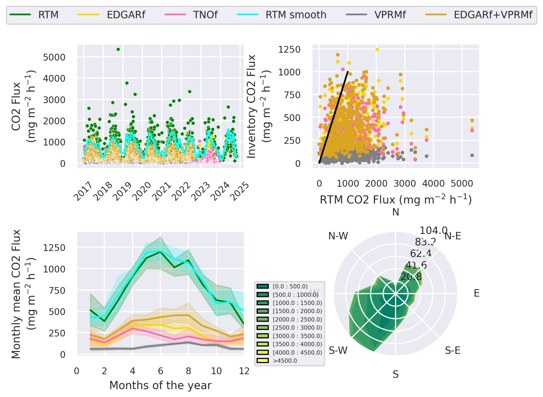
Figure 15 The CO₂ fluxes (RTM), calculated using the STILT_Noah configuration were compared with the smoothed fluxes (RTM smooth), the combined EDGAR, TNO and VPRM inventories using the same footprints for the period 2017–2024 (EDGARf, TNOf and VPRMf, respectively). The top left panel shows all the selected nocturnal fluxes (colored dots), the top right panel shows the correlation between the RTM fluxes and the inventory estimates. The bottom left plot shows the seasonal cycles of the fluxes while the bottom right plot shows the flux repartition over the windrose with the flux intensity as the color scale and its frequency on the axial axe.

4.7 CO₂ fluxes

Contrary to the other gases, CO₂ is also strongly influenced by biogenic emissions not represented in EDGAR or TNO. This is why we also used VPRM. Figure 15 shows the fluxes of CO₂ calculated using the STILT_Noah configuration with the footprints. As for CH₄, the smoothed data, trend and growth rate are shown on Fig. 12, albeit on the bottom right panel. No trend is observed. Looking at the RTM calculated fluxes, we observe a clear seasonal pattern with a minimum in winter and a maximum in summer mostly visible on the bottom left panel. Indeed, we are looking here at nocturnal fluxes without photosynthesis (i.e., with respiration only). The respiration as shown in Belviso et al. (2022), Figure 4, modeled for Saclay over 2015 to 2021, presents a seasonal cycle with a maximum in summer and minimum in winter, an average of 130 $\mathrm{mg}\mathrm{C}{\mathrm{0}}_{\mathrm{2}}{\mathrm{m}}^{-\mathrm{2}}{\mathrm{h}}^{-\mathrm{1}}$ and an amplitude of about 200 $\mathrm{mg}\mathrm{C}{\mathrm{0}}_{\mathrm{2}}{\mathrm{m}}^{-\mathrm{2}}{\mathrm{h}}^{-\mathrm{1}}$. The amplitude of the smoothed RTM fluxes is on average 750 $\mathrm{mg}{\mathrm{m}}^{-\mathrm{2}}{\mathrm{h}}^{-\mathrm{1}}$ so only a third would be accounted for the respiration. Several reasons can explain the difference, first the seasonal respiration in Belviso et al. (2022) is shown only for one grid pixel while in our study, we aggregate the fluxes for the station footprint, where there could be higher gradients of respiration. Secondly, there is of course the anthropogenic contribution of CO₂ as Saclay is a peri-urban site within the influence of the Paris region. The average estimate from EDGARf is 244 $\mathrm{mg}\mathrm{C}{\mathrm{0}}_{\mathrm{2}}{\mathrm{m}}^{-\mathrm{2}}{\mathrm{h}}^{-\mathrm{1}}$ versus 867 $\mathrm{mg}\mathrm{C}{\mathrm{0}}_{\mathrm{2}}{\mathrm{m}}^{-\mathrm{2}}{\mathrm{h}}^{-\mathrm{1}}$ for the RTM. TNOf presents even lower values than EDGARf with an average of 197 $\mathrm{mg}\mathrm{C}{\mathrm{0}}_{\mathrm{2}}{\mathrm{m}}^{-\mathrm{2}}{\mathrm{h}}^{-\mathrm{1}}$. On the figure, we see that EDGARf and VPRMf combined reproduce fairly well the baseline and winter fluxes estimated by the RTM. However, in summer, the RTM fluxes can be two to 3 times higher. This is highlighted in the top right panel where the underestimation is clear for all the bottom-up inventories. The lower right panel shows the higher values coming from the north-east as for CH₄.

The RTM values is higher than the value found for 2002–2007 in (Messager, 2007) of 545 $\mathrm{mg}\mathrm{C}{\mathrm{0}}_{\mathrm{2}}{\mathrm{m}}^{-\mathrm{2}}{\mathrm{h}}^{-\mathrm{1}}$. For the two inventories, transportation, industry and stationary combustion are the three main sources with about the same proportions for both.

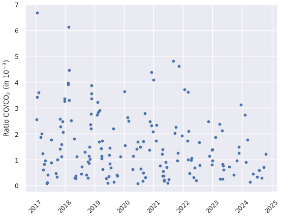
Figure 16 $\mathrm{CO}/{\mathrm{CO}}_{\mathrm{2}}$ ratio from 2017 to 2024 calculated over the common days where both CO and CO₂ fluxes were estimated.

If we look at the $\mathrm{CO}/{\mathrm{CO}}_{\mathrm{2}}$ ratio shown on Fig. 16, we see that in summer, the ratio is below 1.5 × 10⁻³ showing a low influence from the anthropogenic sources and a higher one from the biogenic sources (Ammoura et al., 2014, 2016; Gamage et al., 2020). This seems to point towards a misrepresentation of the biogenic fluxes from this VPRM version within our footprint. This is supported by Lian et al. (2023) where the authors show that the nighttime biosphere signals during the growing season are not well reproduced by the VPRM model for the Ile-de-France region where Saclay is located.

5 Conclusions

This study presents up to 8 years of CO₂, CH₄, CO and N₂O fluxes at Saclay, France from 2017 to 2024 (Yver Kwok, 2025). The fluxes have been calculated using the radon tracer method. An interactive tool has been developped. The RTM has been combined with the latest radon flux maps from the traceRadon project and the STILT footprints as calculated in the ICOS Carbon Portal. A mask on the footprint has been added to correct the 10 d long backtrajectories and thus reproduce the effect of a 5 to 10 h long backtrajectory. A preliminary study focused on CH₄ and 2 months in 2019 helped define the best parameters to use for Saclay. To apply this tool to other stations, it would be necessary to adjust the mask and potentially the nocturnal window. An automatic selection of the sunset–sunrise period could be a development in the future.

In this study, we highlighted the importance of using radon standardized data as well as the impact of the radon exhalation rate maps that remains the main factor of uncertainties in the method despite recent improvements. We also showed that a simple radon decay correction is sufficient to yield accurate results.

In Sect. 4, the method has been applied to up to 8 years of data and four gases.

We found that the average RTM estimates and their variability are 867 ± 565, 1.10 ± 0.89,1.01 ± 1.05 and 0.094 ± 0.118 $\mathrm{mg}{\mathrm{m}}^{-\mathrm{2}}{\mathrm{h}}^{-\mathrm{1}}$ for CO₂, CH₄, CO and N₂O, respectively.

CH₄, N₂O and CO are in fair agreement with the inventories, though with higher values. N₂O differences most probably come from the lack of seasonality in EDGAR inventory. CO₂ fluxes are about 5 times higher than anthropogenic and biogenic fluxes from EDGAR and VPRM combined. The differences mainly occur during summer, and the $\mathrm{CO}/{\mathrm{CO}}_{\mathrm{2}}$ ratio points toward a misrepresentation of the biogenic fluxes by the VPRM version used here.

The literature for either older measurement close to Saclay, or recent measurements in Germany and Netherlands agree fairly well with our findings notwithstanding the difference in the local environment like for methane in the Netherlands where dairy farming is much more prominent than at Saclay.