Aircraft in-situ measurements from SOCRATES constrain the anthropogenic perturbations of cloud droplet number

Aerosol-cloud interactions (ACI) in warm clouds alter reflected shortwave radiation by influencing cloud microphysical and macrophysical properties. The variable of state controlling ACI is the cloud droplet number concentration (N_d). Here, we examine the perturbations in N_d due to anthropogenic aerosols (ΔN_{d, PD-PI}) using a perturbed parameter ensemble (PPE) hosted in the sixth Community Atmosphere Model (CAM6). Surrogate models are created for the CAM6 PPE outputs and are used to generate 1 million model variants of CAM6 by sampling 45 sources of parameter uncertainty. The range of uncertain physical parameters related to ACI are constrained with observations of aerosol and cloud properties from SOCRATES. The likely range of uncertain parameters and the associated range of ΔN_{d, PD-PI} are more strongly constrained with observations of N_d relative to observations of cloud condensation nuclei. We conduct sensitivity tests of how constraints on ΔN_{d, PD-PI} are affected by systematic uncertainties in observations and our limitations in our surrogate models created for CAM6 PPE outputs. Based on this, we provide guidance on the impact of reducing systematic uncertainty in airborne microphysical observations and in surrogate models.

1 Introduction

Clouds play an essential role in setting Earth's top of atmosphere energy flux by reflecting incoming shortwave radiation back to space. Aerosols are important for cloud formation as they serve as cloud condensation nuclei (CCN) for water vapor to condense onto. CCN make cloud droplet formation possible in atmospheric conditions. Aerosols from anthropogenic emissions alter cloud droplet number concentration (N_d) by acting as CCN, enhancing cloud reflectivity (Twomey, 1977). The change in reflected shortwave radiation (i.e., radiative forcing: RF in W m⁻²) through changes in N_d is referred to as the instantaneous radiative forcing due to aerosol-cloud interactions (IRFaci). According to the formulation in Bellouin et al. (2020), IRFaci is given by

$$\begin{array}{}\text{(1)}& \mathrm{IRFaci}={\left.{\displaystyle \frac{\partial R}{\partial \ln N_{\mathrm{d}}}}\right|}_{{\mathrm{LWP}}_{\mathrm{c}},C}\cdot \mathrm{\Delta }\ln N_{\mathrm{d}}\end{array}$$

where R is the net radiative flux. LWP_c is the in-cloud liquid water path (LWP) and Δln N_d is the fractional perturbation in N_d (Ghan et al., 2016; Bellouin et al., 2020). The vertical line in the partial derivative denotes LWP_c and cloud fraction (C) are held constant (Bellouin et al., 2020). With changes in N_d, cloud macrophysical properties can be altered in response to changes in cloud microphysics, such as cloud lifetime, liquid water content and cloud cover (Ackerman et al., 2004). The RF caused by modifications to cloud macrophysics is referred to as aerosol-cloud adjustment and is given by

$$\begin{array}{}\text{(2)}& {\mathrm{RF}}_{\mathrm{adjustment}}=\left({\displaystyle \frac{\partial R}{\partial C}}{\displaystyle \frac{\mathrm{d}C}{\mathrm{d}\ln N_{\mathrm{d}}}}+{\displaystyle \frac{\partial R}{\partial {\mathrm{LWP}}_{\mathrm{c}}}}{\displaystyle \frac{{\mathrm{dLWP}}_{\mathrm{c}}}{\mathrm{d}\ln N_{\mathrm{d}}}}\right)\cdot \mathrm{\Delta }\ln N_{\mathrm{d}}\end{array}$$

The sum of radiative forcing from IRFaci and aerosol-cloud adjustment is termed effective RF due to ACI (ERFaci), which can be expressed as

$$\begin{array}{}\text{(3)}& \begin{array}{rl}& \mathrm{ERFaci}=\\ & ({\left.{\displaystyle \frac{\partial R}{\partial \ln N_{\mathrm{d}}}}\right|}_{{\mathrm{LWP}}_{\mathrm{c}},C}+{\displaystyle \frac{\partial R}{\partial C}}\cdot {\displaystyle \frac{\mathrm{d}C}{\mathrm{d}\ln N_{\mathrm{d}}}}+{\displaystyle \frac{\partial R}{\partial {\mathrm{LWP}}_{\mathrm{c}}}}\cdot {\displaystyle \frac{{\mathrm{dLWP}}_{\mathrm{c}}}{\mathrm{d}\ln N_{\mathrm{d}}}})\\ & \cdot \mathrm{\Delta }\ln N_{\mathrm{d}}\end{array}\end{array}$$

Recent assessments place ERFaci as the largest uncertainty in anthropogenic climate forcing. This uncertainty also complicates efforts to infer climate sensitivity from the historical record, as the cooling from ACI can mask the warming effects of greenhouse gases (GHGs) (Bellouin et al., 2020; Forster, 2016; Watson-Parris and Smith, 2022).

Earth system models (ESMs) are essential for estimating ERFaci as they can estimate the unobservable preindustrial baseline of the atmosphere (Carslaw et al., 2017; Wall et al., 2022). However, ESMs are uncertain in their representations of aerosols and their climate effects. This uncertainty can be related to structural uncertainty (what processes to include in a model) (Regayre et al., 2023) and parametric uncertainty (how the values of parameters in the mathematical representation of processes are set in the ESM) (Regayre et al., 2018). The uncertainties in ERFaci related to parametrizations of unresolved aerosol processes, emissions, and cloud microphysical processes within a single model can be as large as the spread across models with different model structures. This supports the utility of understanding parametric uncertainties (Johnson et al., 2018). A commonly used method is to employ a perturbed parameter ensemble (PPE). This method involves exploring many possible parameter combinations across their uncertainty range to quantify the range of possible outcomes. The plausible range of ERFaci can be estimated using a set of parameter combinations, provided there is good agreement between observations and the model simulations generated by those parameter combinations (Regayre et al., 2018).

Wood (2012) argues that the variable of state (or most important variable) in understanding ACI is the N_d. Effectively, changes in N_d play a pivotal role in governing cloud radiative and macrophysical behavior. This means that to reduce uncertainty in ERFaci, constraining the anthropogenic perturbation to N_d is essential as both IRFaci (Eq. 1) and aerosol-cloud adjustment (Eq. 2) scale with change in N_d (Bellouin et al., 2020; Song et al., 2024).

One obstacle in seeking an observational constraint on the N_d response to anthropogenic aerosol is that the processes driving the N_d response primarily occur at the microscale and the result of these processes poses observational challenges. Past studies have used observations of N_d from spaceborne remote sensing to constrain the change in N_d during historical periods, achieving consistent observational constraints across different host models using the same observations (McCoy et al., 2020; Song et al., 2024; Gryspeerdt et al., 2016). However, observations of aerosol and cloud microphysical properties from remote sensing are known to have uncertainties arising from factors such as assumptions about particle size distributions, cloud microphysics, and radiative transfer models used in the retrieval process (Grosvenor et al., 2018; Zhang et al., 2016; Gryspeerdt et al., 2022).

In-situ measurements provide direct measurements of aerosol and cloud microphysical properties without reliance on retrieval algorithms or assumptions used in remote sensing. It also measures more detailed microphysical properties such as aerosol size distribution, chemical composition, and cloud droplet number concentration and size distributions. However, in-situ measurements can suffer from a wide variety of instrument biases and limitations and the impact of these limitations on our ability to use them for climate studies is not well characterized. For instance, instruments used for measuring aerosol and cloud properties can only detect subsets of the full particle distribution due to their limited sampling volume, and they cannot measure the full spectrum of particle sizes (Lance et al., 2010). In-situ measurements from aircraft occur with a much smaller footprint than a typical ESM and are often targeted towards features that make them not representative to compare to an ESM grid cell (Field and Furtado, 2016). Additionally, by their nature aircraft campaigns have minimal global coverage and it is unclear how effective a constraint on global model behavior they provide.

In this paper, we focus on characterizing an observational constraint on the change in N_d during the historical period (ΔN_{d, PD-PI}) based on in-situ measurements from a single campaign to illustrate the utility of combining two key tools: ESMs and airborne observations of microscale properties. We expand on previous work (Gettelman et al., 2020) by examining parametric uncertainty across a single ESM (i.e. using a PPE) and characterizing what we can learn from an airborne campaign and expanding on previous PPE work leveraging surface observations of aerosol properties (Regayre et al., 2020). We use observations of both aerosol and cloud properties from aircraft in-situ measurements. We address the following question: (1) do aerosol or cloud measurements better constrain global cloud microphysical behavior? (2) can sparse in-situ measurements produce constraints on cloud microphysical behavior on a global scale? (3) how sensitive is the observational constraint on ΔN_{d, PD-PI} to observation uncertainties? We provide this analysis with the goal of (i) showing the connection between in-situ measurements and our understanding of climate (Regayre et al., 2020) and (ii) characterizing where to expend effort in terms of sampling with in-situ measurements and model development.

2 Materials and Methods

2.1 The CAM6 Perturbed parameter ensemble

We use the Community Atmosphere Model version 6 (CAM6), which is the atmosphere component of the Community Earth System Model version CESM-2.0 (Danabasoglu et al., 2020). The CAM6 model uses a two-moment microphysics scheme for stratiform clouds, with liquid, ice, rain, and snow hydrometeors calculated as prognostic variables, allowing CAM6 to explicitly represent the aerosol indirect effect (Gettelman and Morrison, 2015; Gettelman et al., 2015).

We leverage a perturbed parameter ensemble (PPE) hosted in CAM6 (Eidhammer et al., 2024). A PPE is a large set of simulations based on the structure of a single ESM (e.g., CAM6) with a different combination of parameter values to examine parameter uncertainty (Lee et al., 2011; Carslaw et al., 2013). The CAM6 PPE is fully described in Eidhammer et al. (2024). CAM6 is run at the standard resolution of 1.25°×0.9375° resolution. Briefly, 262 model simulations (i.e., 262 parameter combinations) of CAM6 sample 45 sources of uncertainty in the parameterizations for cloud, precipitation, convection, boundary layer, and aerosol processes. The 45 parameters are simultaneously perturbed using Latin Hypercube within the plausible range of realistic values based on expert-elicitation. We examine 203 ensemble members out of 262 integrated. The remaining 59 members were excluded based on criterion: (1) the linear regression slope of N_d to CCN in log space ($\mathrm{d}\ln N_{\mathrm{d}}/\mathrm{d}\ln \mathrm{CCN}$) is less than 0; (2) the correlation coefficient between N_d and CCN is less than 0.3. The two criteria are used to exclude PPE members that are too far outside the observational constraint behaviors (i.e., the Southern Ocean field campaign measurements analyzed in Fig. 14 in McCoy et al., 2021). Following Song et al. (2024), we also exclude PPE members that simulate too much ice in tropics, which is inconsistent with satellite observations (King et al., 2013).

2.2 Model Configuration

Two scenarios are simulated and each of them use the same parameter combinations – consistent with previous studies (Song et al., 2024). First, 2-year global simulations saved at monthly-mean are completed for pre-industrial (PI) and present-day (PD) emissions. PI and PD aerosol emission scenarios are integrated from 2019 to 2020 so anthropogenic perturbations in N_d can be calculated over global coverage by taking the difference between PI and PD. The atmosphere is nudged to horizontal winds and temperature and sea surface temperature and sea ice fraction are prescribed from observations. Wind and temperature fields are nudged to the Modern-Era Retrospective analysis for Research and Applications, Version 2 (MERRA2) reanalysis (Bosilovich et al., 2015) with 24 h relaxation time. MERRA2 output is interpolated to CAM6 vertical resolution with standard 32 vertical levels from the surface to 3 hPa following Gettelman et al. (2020). Previous studies have shown the CAM6 PPE produces a wide range of perturbations in cloud microphysics (e.g., ΔN_{d, PD-PI}) and cloud macrophyiscs (ΔLWP_PD-PI). In this study, we focus on diagnosing the parametric effects on cloud microphysical responses to anthropogenic aerosols from different parameter combinations using the PPE.

In addition to the two-year integrations of the PPE used to calculate anthropogenic perturbations in N_d, the PPE is integrated over short periods consistent with the Southern Ocean Clouds, Radiation, Aerosol, Transport Experimental Study (SOCRATES) field campaign based from Hobart, Tasmania (McFarquhar et al., 2021) (Fig. 1). The SOCRATES campaign occurred over the midlatitude Southern Ocean (SO) during austral summer and was dominated by a series of frontal systems, postfrontal stratocumulus decks, and cyclonic activity typical of the storm track region (McFarquhar et al., 2021). Model outputs are saved along flight tracks over SOCRATES and is sampled at 1 min resolution following Gettelman et al. (2020). It applies atmospheric nudging to horizontal winds and temperature, consistent with global simulation with PI and PD aerosol emissions scenarios, but nudged to the period of January–March 2018 when the aircraft observations were conducted. The behavior of the default parameter configuration in CAM6 has been characterized using this approach in Gettelman et al. (2020), McCoy et al. (2021), McCluskey et al. (2023), Zhou et al. (2021).

Previous studies have shown that the CAM6 PPE, configured with 2-year global simulations, produces a wide spread in present-day (PD) cloud microphysical (N_d) and macrophysical (LWP) properties. The mean-state PD values have been shown to fall within the observational range derived from satellite remote sensing (Song et al., 2024). Additionally, CAM6 simulations along flight tracks using the default parameter configuration reproduce many features of in-situ observations, including cloud phase, cloud location, and boundary layer structure (Gettelman et al., 2020). These results give us confidence that at least some members of the nudged PPE simulations provide a physically plausible baseline in terms of cloud microphysical and macrophysical properties. In this study, we focus specifically on microphysical properties.

2.3 Aircraft Sampling

We examine in-situ airborne observations taken from SOCRATES as our observational constraint (McFarquhar et al., 2021). The importance of the Southern Ocean (SO) to understanding the global anthropogenic contribution to N_d has been shown in several previous studies (Carslaw et al., 2013; McCoy et al., 2020). The National Science Foundation Gulfstream-V (GV) aircraft was deployed during January–March 2018 for SOCRATES. There were 15 flights sampling data from 42 to 62° S with aerosol and cloud properties sampled at 1 Hz frequency. The GV was equipped with a variety of sensors and instruments. In this work, N_d from the cloud droplet probe (CDP) and aerosol number concentrations from the ultra-high sensitivity aerosol spectrometer (UHSAS) are examined. We focus on accumulation mode aerosols, with diameters ranging from 0.1 to 1 µm, reported as UHSAS100 in this paper following McCoy et al. (2021). Accumulation mode aerosol usually accounts for most of the surface area of aerosols and is a good estimate of the CCN concentration for stratocumulus updraft velocities (Seinfeld and Pandis, 2016).

With a focus on low-level, liquid cloud, we restrict the aircraft measurements of aerosol and cloud to be below 2 km. As in previous studies (McCoy et al., 2021), in-situ aircraft aerosol measurements are discarded when the liquid water content (LWC) from the CDP exceeds 0.001 g m⁻³, along with the subsequent 10 s after cloud detection. This is to avoid measurement contamination from cloud (McCoy et al., 2021). In-cloud N_d measurements are restricted to regions where the LWC from the CDP is greater than a threshold (0.1 g m⁻³) following McCoy et al. (2021). Because the observations of aerosols and in-cloud N_d that are considered valid for use are taken at different locations, direct comparison is challenging due to inconsistencies in spatial and temporal coverage. To make comparisons between N_d and aerosol observations, we bin the aircraft measurements by 2 min in duration and 50 m in altitude so that aerosols and N_d can be compared in the same bin. Only bins with at least ten 1 Hz flight observations are considered valid composites for use. Median values of aerosol concentration and N_d are computed for each bin for observations from each flight following McCoy et al. (2021). The instrument limitation inevitably forces us to look either at small clouds or cloud edges, where both the measurements of aerosol and cloud are valid for use. This has minimal impact on our comparison between models and observations as we colocate model output with observations as detailed in Sect. 2.4.

In this study, we focus exclusively on low-level, liquid clouds simulated by the stratiform (large-scale) cloud microphysics scheme (MG2) in CAM6, as CAM6’s convective scheme does not include prognostic microphysical variables such as N_d, which is a key quantity in our analysis. As such, all N_d values analyzed in this study originate from the stratiform cloud scheme. Furthermore, we limit our comparison with aircraft observations to altitudes below 2 km, corresponding to the marine boundary layer and excluding a large potion of clouds formed by deep convection (Kang et al., 2024). The majority of simulated N_d in CAM6 is also concentrated below 2 km (Zhou et al., 2021). The convective scheme, while it may be triggered during postfrontal cloud conditions, does not contribute to N_d in CAM6. The convective scheme can contribute to precipitation, while this is beyond the scope of analysis in the present study.

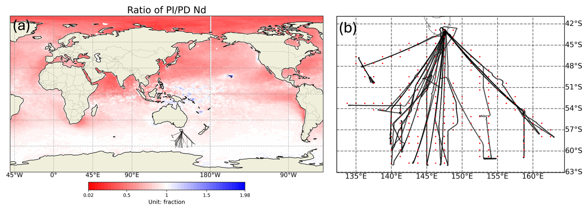
Figure 1 Maps of SOCRATES mission flight tracks from the NSF G-V aircraft. (a) Location of the SOCRATES aircraft sampling and the ratio of preindustrial to present day N_d shown in colors. The ratio is computed as $\frac{\text{PI Nd}}{\text{PD Nd}}$ using the preindustrial and present-day simulations run for two years configured with default CAM6 parameter setting. Ratios less than 1 indicate anthropogenically polluted regions. (b) Comparison of sampling of aircraft measurements (black line) with CAM6 grid point centers (red dots). Along-flight-track simulations are run for January–March 2018, covering late austral summer into early autumn.

2.4 Comparison Between Model data and Observations

The default configuration of CAM6 has been extensively evaluated in Gettelman et al. (2020) and McCoy et al. (2021) and has been shown to be able to reproduce many features consistent with in-situ observations in Gettelman et al. (2020). Here, we examine a PPE that is hosted in the same model evaluated in previous studies (McCoy et al., 2021; Gettelman et al., 2020). The CAM6 model parameterization and the prior distribution of parameters (i.e., 217 sets of parameter combinations) in the PPE (Eidhammer et al., 2024) produce simulated aerosol and cloud properties that we can compare with observations to evaluate how process representation impacts aerosol-cloud interactions. Here, we focus on microphysical quantities that are available from in-situ measurements but hard to observe from spaceborne remote sensing.

N_d is directly available from both CAM6 and in-situ measurements from the CDP. CAM6 in-cloud N_d is calculated as N_d divided by liquid cloud fraction (when cloud fraction ≤ 1  %, we set N_d=0). This cloud fraction threshold is smaller than the one used in McCoy et al. (2021) as we found it retains more flight composites but does not significantly change the results of our analysis (Fig. S1 in the Supplement).

CCN is a subset of aerosols that can be activated to cloud droplets at a given supersaturation. CAM6 outputs CCN at a set of fixed supersaturations. Here, we look at supersaturation at 0.2 %. It is found that observed CCN at 0.2 % supersaturation (CCN02) has an one-to-one relationship with accumulation mode aerosol (e.g., UHSAS100) measured over SOCRATES (McCoy et al., 2021). Following previous work (McCoy et al., 2021), we use UHSAS100 as a proxy to CCN02 over SOCRATES as UHSAS100 lies very close to the one-to-one line with CCN02. This supersaturation level is shown to be representative of marine low-level stratocumulus (Hudson and Svensson, 1995).

To make comparisons between the modeled and observed N_d and aerosol properties, model data are colocated to observations by linearly interpolating to temporal and spatial locations from the 2 min × 50 m observational composites following McCoy et al. (2021). Our comparison between observations and models follows two strategies. First, model outputs (CCN and N_d) are confronted with in-situ observations for collocated bins (flight track composites) along flight tracks for each simulation ensemble. This method allows for the evaluation of simulated CCN, N_d, and the inferred efficiency of aerosol activation ($\frac{\mathrm{d}{N}_{\mathrm{d}}}{\mathrm{dCCN}}$) relative to observations within individual PPE members. The results are discussed in Sect. 3.1. Second, campaign-means of CCN and N_d are calculated for each PPE ensemble and compared with campaign-means of CCN and N_d calculated from in-situ observations. In this approach, we evaluate aerosol activation efficiency across the CAM6 PPE members (run with different parameter sets) and use campaign-means of in-situ aerosol properties and N_d to constrain the CAM6 PPE (Sect. 3.3.3).

The intention of taking the campaign-mean is to reduce random error by averaging over a large number of samples. However, there remains potential sources of systematic error. One possible source of systematic error is from differences in sampling between the observations and the model (e.g. if the pilot only flew through clear air and avoided cloud). Sampling during airborne campaigns may have some systematic sampling biases as discussed in Field and Furtado (2016). Output from CAM6 is representative of an average within the grid box of the model, whereas flight patterns in a similar-sized domain may not be sampling randomly (e.g. focusing on convective cores). We believe that this is a minimal concern for SOCRATES. The SOCRATES flight pattern was designed to focus on cold sectors of cyclones and synoptically uplifted aerosol layers, but followed a random sampling pattern in those large-scale features (McCoy et al., 2021). In addition to any systematic errors from sampling strategy, instrument error inherent in the CDP introduces additional uncertainties in the measurements of N_d. CDP measures cloud droplets within a specific size range (i.e., 2 to 50 µm in diameter). It has limitations regarding droplets that fall outside its designed size range. Coincidence errors may occur when multiple droplets pass through the sensor's detection volume but is counted as a single droplet. The impact of observational uncertainty on the model constraints is examined in in Sect. 3.4.

Another potential source of systematic uncertainty may arise from the use of UHSAS100 as a proxy to CCN02 over SOCRATES. While a near one-to-one relationship between UHSAS100 and CCN02 has been reported for the SOCRATES campaign (McCoy et al., 2021), the campaign-mean ratio of CCN02 to UHSAS100 is approximately 1.08 (±0.3), based on the median and interquartile range of the CCN02 : UHSAS100 ratio uncertainty shown in their Fig. S2. This suggests that UHSAS100 may underestimate CCN02 by 8 % on average. Moreover, the activation diameter for SO aerosol is typically below 100 nm at 0.2 % supersaturation, and likely closer to 80 nm for the aerosol population sampled during SOCRATES (Fossum et al., 2018; Mallet et al., 2025). This suggests that USHS100 may introduce an even greater underestimation of CCN02 compared to UHSAS100. To reflect the potential offset between UHSAS100 and CCN02, we conducted sensitivity tests by increasing the observed “CCN” by 8 % and 40 %, representing the lower and upper bounds of the CCN02 to N100 ratio uncertainty, to examine how this affects our results (Sect. 3.3.3).

Having discussed uncertainty in the observations, we can turn our attention to uncertainty in the representation of processes in models. While the PPE samples a large number of possible representations of the underlying physics, it is still quite sparse (Lee et al., 2011). To systematically explore parametric uncertainty across the PPE, we build emulators (surrogate models) for the campaign-mean N_d and CCN using Gaussian Process (GP) regression (Watson-Parris et al., 2021). Emulators are trained by using the 45 perturbed parameters as inputs and simulation outputs (e.g., campaign-mean N_d and CCN) using a subset of the PPE ensemble as training data. Emulators are trained on the sample of different process representations in the CAM6 PPE data (Fig. S2). The creation and validation of the emulators follows previous literature (Lee et al., 2011; Regayre et al., 2020; Song et al., 2024). With the GP emulators, we sample 1 million model realizations of N_d and CCN (e.g., model variants) with 1 million different combinations of parameter values sampled uniformly across 45 dimensional parameter space.

Model variants are ruled out when they are observationally implausible based on a implausibility measure

$$\begin{array}{}\text{(4)}& I\left(x\right)={\displaystyle \frac{|M-O|}{\left|\text{Error}\right(M\left)\right|+\left|\text{Error}\right(O\left)\right|}}>\mathrm{1}\end{array}$$

where M is the emulator campaign-mean and O is the observed campaign-mean (Regayre et al., 2020). Error(M) and Error(O) denote the deviation from the emulator campaign-mean and observation campaign-mean, respectively. Error(M) comes from emulator uncertainty and the variance Var(M) in the emulator estimate is directly calculated from GP regression. Error(M) is estimated as $\pm \mathrm{1.96}\times \sqrt{\mathrm{Var}\left(M\right)}$. The number of 1.96 is chosen as $\pm \mathrm{1.96}\times \sqrt{\mathrm{Var}\left(M\right)}$ covers approximately 95 % confidence bounds of the emulator uncertainty. Estimating observational uncertainty Error(O) as fractional value is commonly used in observational constraints on models (Johnson et al., 2020; Song et al., 2024). We discuss observational uncertainty in terms of a fractional error f_obs. Finally, we write the implausibility metric I(x) where we account for 95 % uncertainty in the emulator and an arbitrary observational uncertainty as

$$\begin{array}{}\text{(5)}& I\left(x\right)={\displaystyle \frac{|M-O|}{|\sqrt{Var\left(M\right)}\cdot \mathrm{1.96}|+|O\cdot f_{\mathrm{obs}}|}}>\mathrm{1}\end{array}$$

Model variants are excluded when I(x) exceeds 1. An illustration of our constraint process is summarized in Fig. S3.

In this paper, we vary the observational uncertainty by varying f_obs under two conditions: (1) with emulator uncertainty and (2) without emulator uncertainty, to characterize the impact of different sources of uncertainty on our ability to constrain the response of N_d to anthropogenic aerosol. We discuss the impact of different values of f_obs on the model constraint process in Sect. 3.4. Equation (5) is a simplified implausibility metric as in Williamson et al. (2013), Johnson et al. (2020). Here, we only consider observational uncertainty and emulator uncertainty in the comparison between 1 million model variants with observations. Spatial-temporal representation uncertainty and model structural uncertainty are also important as discussed in Johnson et al. (2020). We set the spatial-temporal representation uncertainty to 0 in Eq. (5) as we collocated the model outputs to flight track locations in 2 min × 50 m composites. The characterization of model structural uncertainty is conceptually ambiguous to quantify (Regayre et al., 2023) and is not considered in this work.

2.5 Constraint metric

We conducted sensitivity tests on the observationally plausible 2.5–97.5th percentile range of ΔN_{d, PD-PI} to the emulator and observational uncertainties. The observationally plausible 2.5–97.5th percentile range of ΔN_{d, PD-PI} was calculated with varying presumed observation uncertainties. To reduce noise from imperfect emulators, we conduct another set of sensitivity tests with emulator uncertainties set to 0 (Error(M) = 0) in Eq. (4) in the sensitivity test. The “constraint” is quantified as the reduction in the observational plausible range relative to the prior range predicted from the 1 million model variants. The relative reduction in range is calculated using

$$\begin{array}{}\text{(6)}& \begin{array}{rl}& \text{constraint}=\mathrm{1}-\\ & {\displaystyle \frac{\text{Posterior: }\mathrm{\Delta }{N}_{\text{d,(PD-PI),obs, 97.5}}-\mathrm{\Delta }{N}_{\text{d,(PD-PI),obs, 2.5}}}{\text{Prior: }\mathrm{\Delta }{N}_{\text{d,(PD-PI), 97.5}}-\mathrm{\Delta }{N}_{\text{d,(PD-PI), 2.5}}}}\end{array}\end{array}$$

Where the subscript “obs” denotes the sources of observations that are used for constraints. The posterior range refers to the range of observationally plausible ΔN_{d, PD-PI} at 2.5–97.5th percentiles. The prior range refers the 2.5–97.5th percentile range of ΔN_{d, PD-PI} derived from the original 1-million-member sample. Mathematically, the range of constraint in Eq. (6) should vary between 0 to 1. The greater the magnitude, the better constraints we can achieve.

2.6 Spaceborne observation

In addition to the comparison between aircraft measurements and model outputs saved along flight tracks, we examine the simulated global oceanic mean N_d and confront it with observations. Observations of global oceanic N_d are derived from the Moderate Resolution Imaging Spectroradiometer (MODIS). MODIS is a passive radiometer onboard NASA’s Terra and Aqua satellites. N_d is calculated from MODIS retrievals of effective radius (r_e) and optical depth (τ) assuming an adiabatic cloud (Grosvenor and Wood, 2014). MODIS N_d is calculated for daily means for the period 2003–2015 and is gridded to 1 by 1° resolution as in Grosvenor and Wood (2014). During winter, high-latitude regions (e.g., Arctic, Antarctic) have greater solar zenith angle (SZA), resulting in lower reflected solar radiation, making retrievals of cloud properties (e.g., r_e and τ) less reliable. MODIS N_d is unavailable during wintertime high latitude regions. To ensure consistency in the comparison between MODIS N_d and the model data, N_d data from months and latitudes where MODIS retrievals are unavailable are removed from the ESM dataset. In addition to global oceanic mean N_d from MODIS, we also examine a box region from MODIS with latitude range of 65–42° S and longitude range of 132–165° E, which covers the SOCRATES campaign. MODIS N_d is computed in this box region and compared with campaign-mean N_d from SOCRATES in-situ measurements.

3 Results

As discussed above, previous studies have evaluated CAM6 in terms of its representation of SO aerosol, cloud, and precipitation characteristics using in-situ observations from SOCRATES (McCoy et al., 2021; Zhou et al., 2021; Gettelman et al., 2020; McCluskey et al., 2023). They found that simulated N_d is typically too low in CAM6, which is similar to other ESMs (McCoy et al., 2020). However, finding why the SO N_d is low is complex since N_d is the result of sources and sinks (Wood et al., 2012; McCoy et al., 2020; Kang et al., 2022). To understand what leads to biases in N_d we need to simultaneously consider the impact of multiple processes to tackle the equifinality problem. Briefly, equifinality means multiple combinations of physical processes can result in the same observable state (i.e. N_d).

A common suggestion by previous studies is that investigation of aerosol, cloud, precipitation, glaciation, turbulence and activation processes is needed to understand the source of the model N_d bias (McCoy et al., 2021; Zhou et al., 2021; McCluskey et al., 2023). Here, we examine how different parameter combinations of these processes impact SOCRATES aerosol, clouds, and ACI in CAM6 in Sect. 3.1. By observationally confronting simulations with different parameter combinations, we can evaluate the constrained parameter spaces (Sect. 3.2) and the likely range of observationally-plausible parameter spaces and their associated range of ΔN_{d, PD-PI} (Sect. 3.3).

3.1 CCN, N_d and aerosol activation over SOCRATES in CAM6 PPE

We examine relationships between CCN and N_d across flight composites (50 m × 2 min bin median) within individual PPE members. The number of flight composites valid for CCN-N_d comparisons from SOCRATES in-situ observations is 44 (Fig. 2: red dots). This number is smaller than the results in McCoy et al. (2021) as we choose a lower altitude level for analysis with a focus on warm liquid cloud. The number of colocated flight composites valid for CCN-N_d comparisons for each PPE ensemble member (Fig. 2: black dots) is less than that from observations (red dots) since some flight composites simulates near-zero N_d and are excluded from our analysis. This might be due to the coarse vertical resolution of CAM6 and linear interpolation cannot fully capture the N_d variability in the vertical. Despite the limitations, PPE ensemble members simulate CCN and N_d flight composites that are comparable with observations.

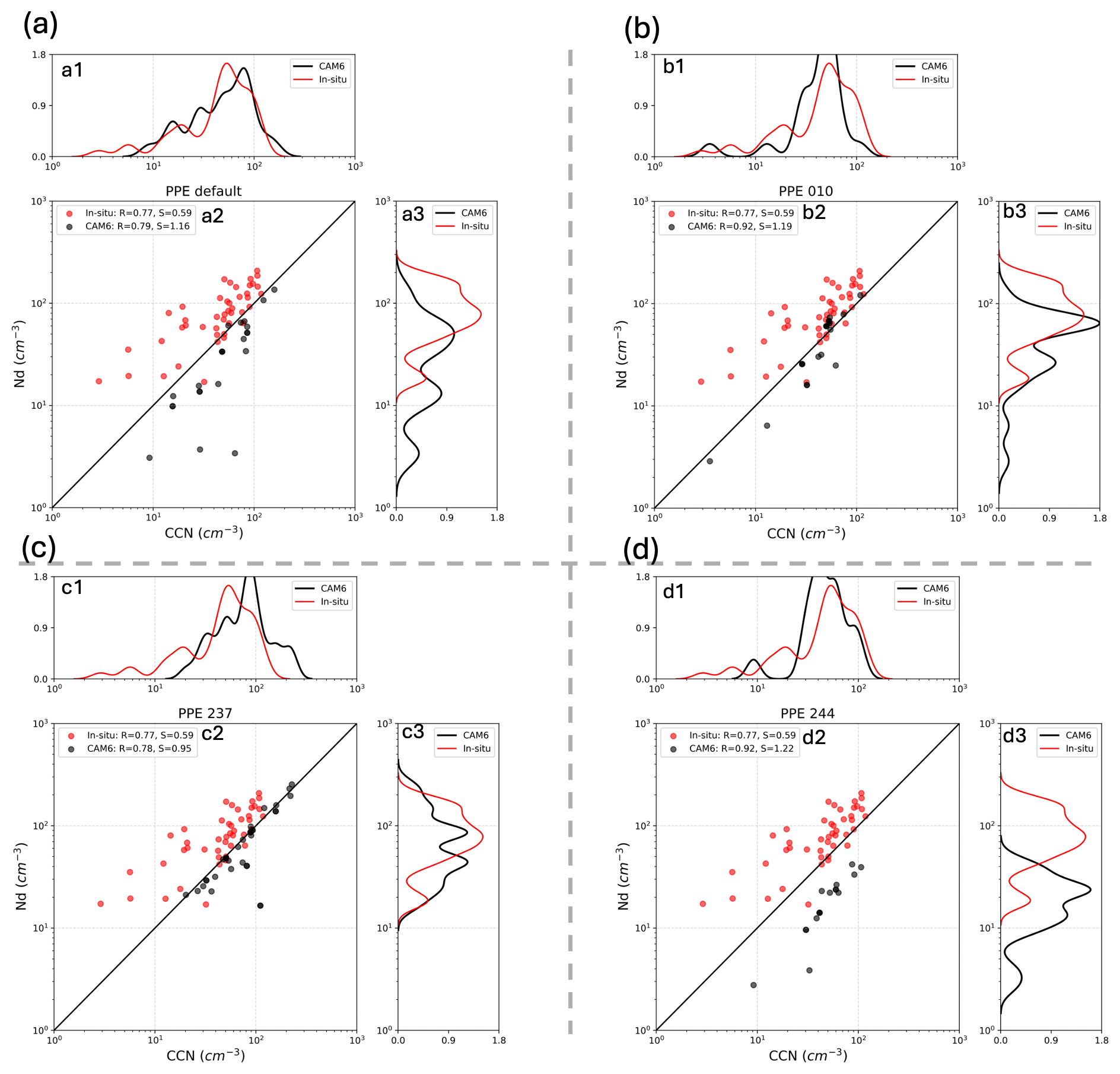
Figure 2 Relationships between SOCRATES CCN and in-cloud cloud droplet number concentration (N_d) from in-situ measurements (red) and CAM6 members (black), based on flight composites along individual flight tracks (scatters). Flight composites are constructed by binning observations into 50 m (altitude) by 2 min (time) bins for each flight. CAM6 PPE CCN and in-cloud N_d are collocated to observation composites (50 m × 2 min bins) by linear interpolation for individual PPE members. Bin medians are taken for comparison with CAM6 models following McCoy et al. (2021). CAM6 in-cloud N_d is computed as N_d divided by liquid cloud fraction (when cloud fraction ≤ 1 %, we set N_d = 0). PDFs of number concentrations of CCN (top) and cloud droplets (right) for matched binned values occurring for CAM6 (black) and observations (red) are shown. (a) Default CAM6 configuration (i.e., PPE simulation for ensemble member 000), (b) PPE simulation for ensemble member 010, (c) PPE 237, (d) PPE 244. PPE members numbered 010, 237 and 244 are chosen to represent cases with varying levels of agreement between the simulated and observed CCN and N_d.

CCN at 0.2 % supersaturation correlates positively with N_d when comparing matched flight composites along individual flight tracks in the PPE (Fig. 2). This is not surprising as we expect CCN at 0.2 % supersaturation to be a reasonable proxy for the aerosol particles that activate to form cloud droplets under typical marine boundary layer updraft conditions, consistent with observations (McCoy et al., 2021). Hereafter, we refer to the simulated CCN at 0.2 % supersaturation from CAM6 simply as CCN for simplicity. Observations of CCN refer to the observed aerosol concentration with diameters ranging from 0.1 to 1 µm from UHSAS100.

Figure 2 shows a subsample of ensemble members with varying levels of agreement with observations, but a positive correlation between CCN and N_d in log space is found for most of the PPE members (i.e., 224 out of 262). However, the linear regression slope of N_d on CCN is high relative to observations for the majority of PPE members (Fig. S4a). Because N_d is a product of both CCN activating into droplets and precipitation removing drops (Wood et al., 2012), a higher CCN-N_d slope in CAM6 does not necessarily indicate a higher simulated aerosol activation efficiency. This diagnostic is broadly telling us that more CCN is required in CAM6 PPE to produce the same amount of N_d through aerosol activation in the presence of coalescence scavenging compared to observations, particularly at low N_d concentration (e.g., Fig. 2a). Lower N_d over SOCRATES is associated with increased precipitation rate and greater contribution of coalescence scavenging in controlling N_d (Kang et al., 2022). The negative correlation between N_d and precipitation rate is also found in the CAM6 PPE (Fig. S5). The high bias in the regression slope of N_d on CCN in CAM6 PPE may indicate a stronger loss in N_d from overestimated coalescence scavenging at low N_d concentration in models. Additionally, the low-biased N_d may also be influenced by an underestimation of subgrid-scale vertical velocity, turbulence intensity, and other dynamical factors that suppress supersaturation and droplet activation. We verify our hypothesis in the discussion of parameter constraints of CAM6 PPE using observations in Sect. 3.2.

Most of the PPE members simulate N_d that is low relative to observations, regardless of whether CCN is underestimated (Figs. S4, 2). One example is the PPE ensemble of 244 of CAM6 where even though the simulated CCN is relatively close to observations, the N_d is still biased low (Fig. 2d). This supports the hypothesis in McCoy et al. (2021) that aerosol biases are not the sole contributors to the low N_d in CAM6, highlighting the importance of other contributing factors.

Although most PPE members exhibit low N_d, there are some members that are close to observations (Figs. S4, 2c). We next compare the PPE with observations to rule out PPE members that are far away from observations (e.g., Fig. 2d) and characterize which parameterized processes are important to ACI over SO.

3.2 CAM6 parameter constraints from SOCRATES measurements

We compare campaign-means of CCN and N_d because averages reduce random errors of aircraft measurements due to instrument noise, atmospheric turbulence, or other transient variations (Schutgens et al., 2021). Unlike random errors, systematic errors such as sensor miscalibration and systematic sampling cannot be reduced by averaging. The model-observation comparison process follows Eq. (5) as detailed in Sect. 2.4.

Observations of CCN and N_d identify and constrain physical processes that are important for ACI (Fig. 3). We show the 10 most constrained parameters out of 45 in Fig. 3. The full list of constrained parameter spaces is shown in Fig. S6. By examining how different parameter values are constrained relative to observables we can try to build an understanding of how different processes drive observables. This also illustrates the problem of equifinality where observed values can be arrived at by combining processes in different ways.

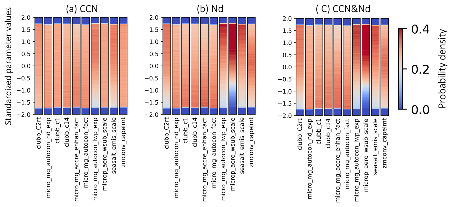
Figure 3 10 parameters with constrained parameter spaces with observations of (a) CCN, (b) N_d and (c) CCN and N_d. Parameter spaces are standardized with mean 0 and variance 1. Warmer colors mean a higher intensity and more data points in that range.

Confronting the PPE with observations of CCN constrains aerosol processes (e.g. sea salt emission) and precipitation processes (e.g. autoconversion, accretion) (Fig. 3a; the detailed parameter explanation is in Table S1 in the Supplement). The sea salt emission scale factor is constrained to higher values, indicating observations of CCN during SOCRATES are consistent with stronger aerosol production in the CAM6 PPE. This is consistent with a lack of aerosol production in CAM6 (McCoy et al., 2021; Zhou et al., 2021).

Constraints on precipitation processes point to the importance of precipitation as an aerosol sink. One of the key parameterization in warm cloud in climate models is the autoconversion, which represents the rate of initial rain formation through collision-coalescence between small cloud droplets.

We can make sense of the relationship between CCN and the autoconversion parameters by looking at how the rate of rain creation through autoconversion works in CAM6. Autoconversion in CAM6 is written as (Khairoutdinov and Kogan, 2000; Gettelman et al., 2015):

$$\begin{array}{}\text{(7)}& {\left({\displaystyle \frac{\partial q_{\mathrm{c}}}{\partial t}}\right)}_{\text{auto}}=a\cdot q_{\mathrm{c}}^b\cdot N_{\mathrm{d}}^{-c}\end{array}$$

where ${\left(\frac{\partial q_{\mathrm{c}}}{\partial t}\right)}_{\text{auto}}$ is the rate of generation of rain from cloud water. The autoconversion rate depends on the cloud droplet concentration (N_d [cm⁻³] in Eq. 7) and cloud water content (q_c [kg kg⁻¹] in Eq 7). a, b and -c are uncertain parameters perturbed in the CAM6 PPE (Table S1). They are micro_mg_autocon_fact, micro_mg_autocon_lwp_exp and micro_mg_autocon_nd_exp, respectively. Selecting parts of parameter space that are consistent with observations of CCN leads to lower autoconversion scale factors (a in Eq. 7) (less efficient rain production by cloud). The effect of larger exponents on liquid water content (b in Eq. 7) on the rain production depends on the relative magnitude of liquid water content q_c. Larger b can result in thicker clouds that precipitate more efficiently under conditions of q_c>1 kg kg⁻¹. A reversed effect can happen under conditions of q_c<1 kg kg⁻¹. The condition of q_c>1 kg kg⁻¹ seems unlikely during SOCRATES campaign observations and model simulations (Khairoutdinov and Kogan, 2000; Gettelman et al., 2020). Overall, this results in a lower rain rate across cloud liquid water content values when the scale factor is minimized and the exponent is maximized for the liquid water content in typical stratocumulus clouds (Fig. S7). The shift to lower rain rate with observational constraints in CAM6 PPE indicates that rain rate and the loss of CCN from precipitation scavenging are overestimated for the majority of members in CAM6 PPE.

Observations of N_d from SOCRATES constrain parameters related to aerosol and precipitation process (Fig. 3b), consistent with the findings in Wood et al. (2012) and Kang et al. (2022), McCoy et al. (2020) that the N_d budget is a function of a source of droplets from CCN and sink from collision-coalescence. The constraint on initial rain formation rate during autoconversion (Eq. 7) and the constraint on the strength of precipitation suppression are consistent with CCN observations (Fig. 3a, b). Broadly, constraints on precipitation formation are consistent with a weaker sink of cloud droplets as well as less cloud droplet removal via precipitation. This supports the hypothesis in Sect. 3.1 that rain rate and the loss of N_d from precipitation scavenging are overestimated for the majority of members in CAM6 PPE. We also want to note that the SO is dominated by supercooled liquid cloud (Gettelman et al., 2020; McCluskey et al., 2023), making the glaciation (Bergeron–Findeisen Process: water vapor deposits onto ice crystals) important in this region. This means that the growth of ice crystals might be an important sink for N_d. However, we believe the N_d loss from freezing is minimal when our analysis is restricted to the altitudes below 2 km. This is because a large fraction of snow melts and contributes to rain precipitation at low altitudes (Fig. 2 in Field and Heymsfield, 2015). Mixed-phase and ice cloud processes are important in initiating rain as most rain is derived from ice that has melted to form rain (Bergeron, 1935). However, the importance of ice processes is not apparent in our process constraint focused on warmer clouds (Fig. S6). McCluskey et al. (2023) examined ice processes over SOCRATES using observations of detailed aerosol and ice nucleating particle (INP) measurements and models (e.g., CAM6), but the process constraints on ice processes with observations of INPs is beyond the scope of this study.

The parameter constraints from observations of N_d are more stringent than the constraints resulting from using observations of CCN. This is consistent with N_d being the emergent product of aerosol and precipitation processes (Wood, 2012). In addition to aerosol and precipitation processes, mechanisms important for aerosol activation are also constrained by N_d observations (Fig. 3b), such as deep convection (e.g., zmconv_capelmt), subgrid velocity (e.g., microp_aero_wsub_scale), and turbulence (e.g., CLUBB: Cloud Layers Unified by Binormals parameters in Table S1), as they play a role in vertical aerosol transport and in generating supersaturation. In particular, microp_aero_wsub_scale is efficiently constrained to higher values, suggesting an underestimated subgrid velocity (i.e., lower updraft speed) that suppresses supersaturation, leading to lower N_d.

Finally, we examine the effect of constraining the PPE using observations of both N_d and CCN. The effect of combining these constraints is similar to the constraint arrived by N_d alone (Fig. 3c). This is consistent with N_d being an emergent property of both aerosol processes and cloud and precipitation processes.

Observations of CCN and N_d during SOCRATES constrain aerosol, precipitation, and cloud processes. In the next section we examine whether the process constraint from observations of CCN and N_d constrains the response of N_d due to anthropogenic aerosol. Precipitation rate would be a useful constraint on the response of N_d as both observations of CCN and N_d constrain precipitation process as discussed in this section. However, the path to including an observational constraint of cloud base precipitation is somewhat opaque and is not included here. Light precipitation rate at cloud base can be retrieved using radar-lidar techniques (Kang et al., 2022), but to provide an apples-to-apples comparison to CAM6 in terms of cloud base precipitation we believe that an instrument simulator is needed (Silber et al., 2022).

3.3 Observationally plausible ΔN_{d, PD-PI} from SOCRATES measurements

As discussed in the previous section, observations of N_d and CCN constrain the range of possible process representations. In turn, these same processes drive the response of N_d to anthropogenic aerosol. This results in a strong correlation between PD N_d and PI N_d (Fig. 4; black line) and by extension the change in N_d between PI and PD (Fig. 4; orange line) in the CAM6 PPE. The fractional change in N_d (Δln N_d) is computed by taking the slope of ΔN_{d, PD-PI} to N_d following the definition from Bellouin et al. (2020). The Δln N_d predicted by the CAM6 PPE (0.23) is greater than the expert elicitation range from Bellouin et al. (2020) (i.e., 0.05 to 0.17) (Fig. 4). The emergent relationship between PD N_d (observable) and the ΔN_{d, PD-PI} (unobservable) with a r-value of 0.95 can be used to constrain the likely range of ΔN_{d, PD-PI} if we know the possible range of PD N_d (observable). As suggested in Klein and Hall (2015), emergent relationships used for constraints require process-level understanding. We explain the emergent behavior from CAM6 PPE (Fig. 4) using a sink-source model of N_d in Sect. 3.3.2.

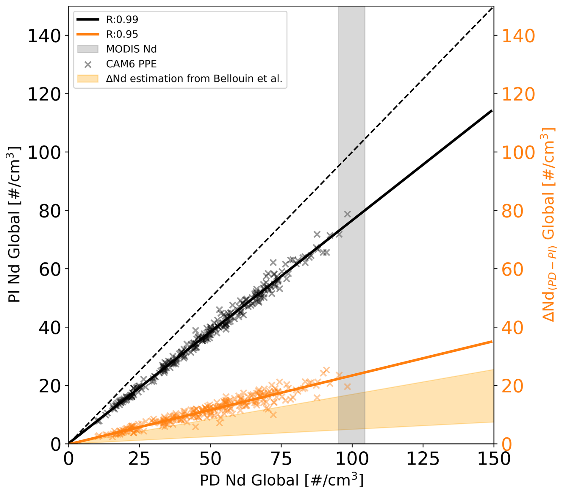
Figure 4 Global oceanic mean of preindustrial (PI) N_d (black) and ΔN_{d, PD-PI} (orange) as a function of present-day (PD) oceanic N_d from CAM6 PPE members (x-shaped markers). The 95 % confidence on the interannual range of global oceanic mean N_d from MODIS is shown in the gray vertical bar. The estimated ΔN_{d, PD-PI} based on the fractional change in N_d (Δln N_d) from Bellouin et al. (2020) is shown in the orange shading.

3.3.1 Constraint using regional measurements

One question is whether SOCRATES, a field campaign over the SO where natural aerosols dominate, can be used to constrain the perturbation in N_d globally. SOCRATES samples natural aerosols and microphysical processes in a pristine environment (McCoy et al., 2021; McFarquhar et al., 2021), but it is not entirely isolated from the effects of anthropogenic aerosol emissions (Fig. 1a). This is consistent with Hamilton et al. (2014), who show that the SO in the present day atmosphere is not always pristine. In addition to aerosol availability acting as a source for the N_d budget, both N_d and natural or anthropogenic aerosols share similar removal pathways through precipitation scavenging (Zheng et al., 2024; Wood et al., 2012; Kang et al., 2022), making the processes sampled during SOCRATES relevant for understanding the N_d perturbations on a global scale.

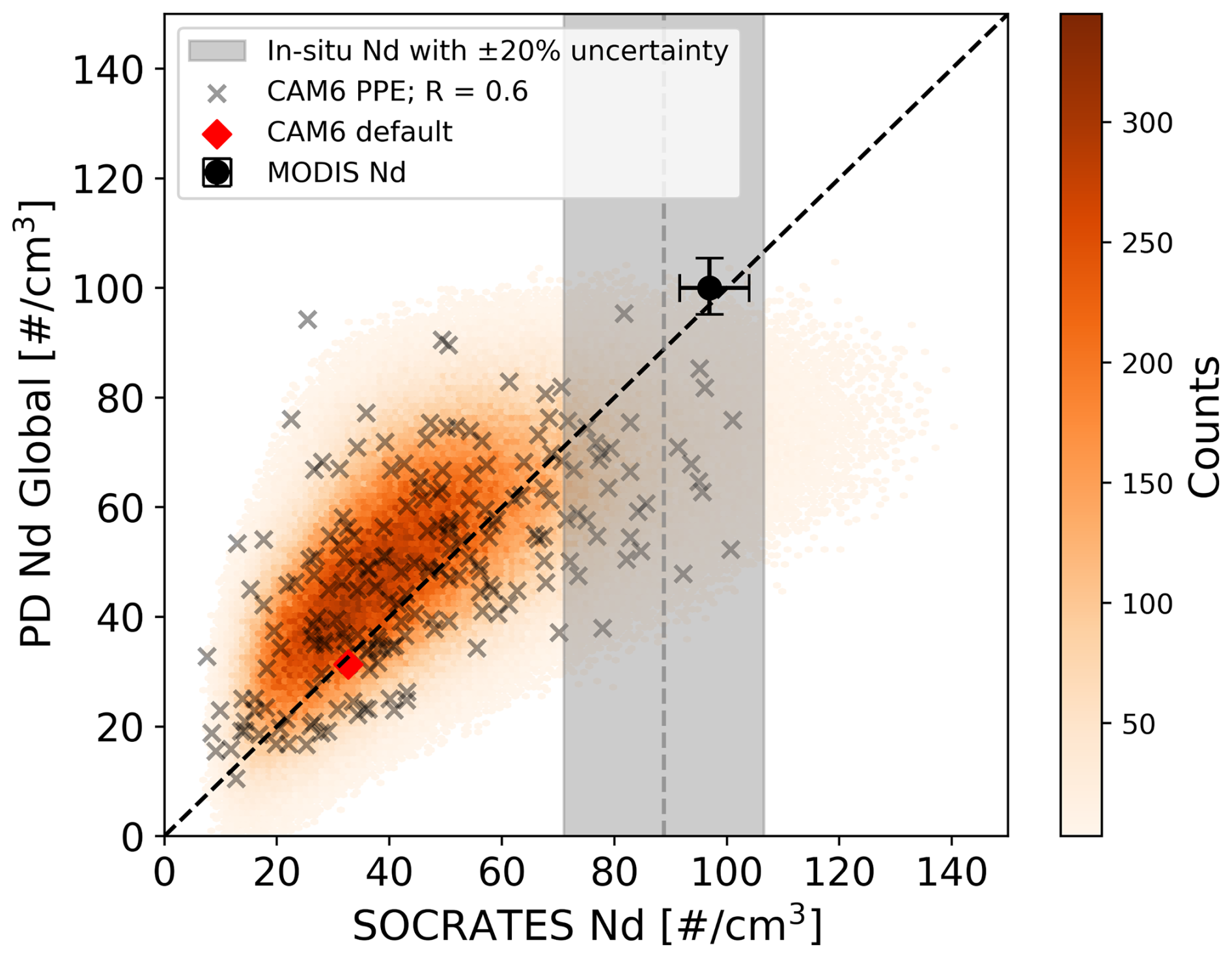
Figure 5 Global oceanic mean of present day (PD) N_d versus SOCRATES campaign-mean N_d from the CAM6 PPE members (x-shaped markers), 1 million emulations from the PPE (orange color shading indicates density) and observations. The black dot shows the observational global-mean N_d and campaign-mean N_d calculated from MODIS, with its 95 % confidence interval based on the interannual range. Observational SOCRATES campaign-mean N_d from SOCRATES in-situ measurements is shown as the vertical dashed line with an uncertainty of ±20 % from the campaign-mean.

Another question is simply how representative is the N_d observed in the sample from SOCRATES of the global mean. Across the PPE, the campaign-mean N_d over SOCRATES correlates with the global, oceanic-mean of N_d with an explained variance of 0.36 across the PPE members (Fig. 5). This positive correlation in N_d is reasonable as processes that govern droplet activation and removal of N_d share similarities over the global ocean and in the SO. The removal of N_d is primarily due to the precipitation scavenging (Wood et al., 2012; Kang et al., 2022). The relationship between the amount of CCN and the resultant N_d contain information about this sink term as well as the transport of CCN to cloud.

The relationship between SOCRATES N_d and the global mean also speaks to the importance of the marine, pristine baseline of aerosol in setting N_d. Previous studies underline the contribution of the oxidation of DMS (McCoy et al., 2015), sea spray (Wood et al., 2012; McCoy et al., 2015; Kang et al., 2022), and transportation of anthropogenic aerosols from continents (Wood et al., 2012; McCoy et al., 2018) to oceanic CCN.

Observational records also show consistency in the amount of N_d between the SO and the globe. Spaceborne observations of SOCRATES campaign-mean N_d and global-mean N_d are relatively consistent (Fig. 5: black dot). In-situ campaign-mean N_d (Fig. 5: gray dashed line) is slightly less than spaceborne observations (Fig. 5: black dot), while the difference is small despite originating from entirely different methodologies.

We hasten to point out that we are not trying to argue that SOCRATES is sufficient to provide a complete picture of global-scale processes. However, SOCRATES does illustrate the utility of investigating even a single field campaign in this framework. Including additional campaigns in future field is likely to provide additional constraint on global-scale processes.

3.3.2 Constraint from present day observations

N_d sampled during SOCRATES contains information for globally-relevant processes (Fig. 5), but do PD observations of aerosol and cloud properties constrain the anthropogenic perturbation in N_d? We find this to be the case in the context of the PPE. To dissect the causes of the relationship between PD N_d and PI N_d, the relationship between PD N_d and ΔN_{d, PD-PI} and the relationship between CCN and N_d we turn to a simple budget model of N_d. Based on Wood et al. (2012), Kang et al. (2022), the N_d budget model is described as a function of source of CCN and sink from precipitation scavenging

$$\begin{array}{}\text{(8)}& N_{\mathrm{d},\mathrm{PD}}={\displaystyle \frac{\left[{\mathrm{CCN}}_{\text{FT}}+\frac{F\left(\mathit{\sigma }\right)U_{\mathrm{10}}^{\mathrm{2.8}}}{D_{Z_i}}\right]}{\left[\mathrm{1}+\frac{hK{P}_{\text{CB}}}{D_{Z_i}}\right]}}\end{array}$$

In Eq. (8), the parameterized source of CCN is from free troposphere CCN_FT and surface contribution $\frac{F\left(\mathit{\sigma }\right)U_{\mathrm{10}}^{\mathrm{2.8}}}{D_{Z_i}}$ (e.g., sea spay aerosol), where F(σ) is the sea spray function that depends on supersaturation (Clarke et al., 2006) and $D_{Z_i}$ is the subsidence rate at cloud top, which is used an approximate for entrainment rate (McCoy et al., 2020). For the precipitation sink term $\frac{hK{P}_{\text{CB}}}{D_{Z_i}}$, h is the cloud thickness, K is a constant that depends on the collection efficiency of cloud droplets and P_CB is the rain rate at cloud base (Wood, 2006). The N_d budget model has been used to predict the N_d amount with confidence over the subtropic and mid-latitudes (Mohrmann et al., 2018; Zheng et al., 2018; Kang et al., 2022).

In this study, we follow the basic source-sink model idea from Wood et al. (2012) but we simplify the N_d budget model to fewer terms for a conceptual understanding of the relationships between variables. The N_d budget model is written as

$$\begin{array}{}\text{(9)}& N_{\mathrm{d}}={\displaystyle \frac{\mathit{\lambda }\cdot \mathrm{CCN}}{\mathrm{1}+k_{\mathrm{remo}}\cdot P_{\mathrm{CB}}}}\end{array}$$

Instead of parameterizing CCN source from free troposphere CCN_FT and surface contribution $\frac{F\left(\mathit{\sigma }\right)U_{\mathrm{10}}^{\mathrm{2.8}}}{D_{Z_i}}$, we characterize CCN source as λ⋅CCN, where λ is a scale factor that accounts for the amount of CCN that can be activated to cloud droplets depending on the vertical updraft, relative humidity, size and hygroscopicity of CCN, etc. λ varies from 0 to 1. For precipitation sink term $\frac{hK{P}_{\text{CB}}}{D{}_{Z_i}}$, we simplified it as k_remo⋅P_CB, where k_remo equals to $\frac{hK}{D{}_{Z_i}}$. It accounts for the rate of loss of N_d from precipitation. To estimate k_remo, we set K=2.25 m² kg⁻¹, subsidence rate D_Zi=4 mm s⁻¹ following Wood et al. (2012), Kang et al. (2022), McCoy et al. (2020). Cloud thickness h is set to 300 m, which is a typical magnitude for marine clouds (Wood, 2012). Changing cloud thickness h to smaller (e.g., 100 m) or larger values (e.g., 500 m) does not significantly change our results.

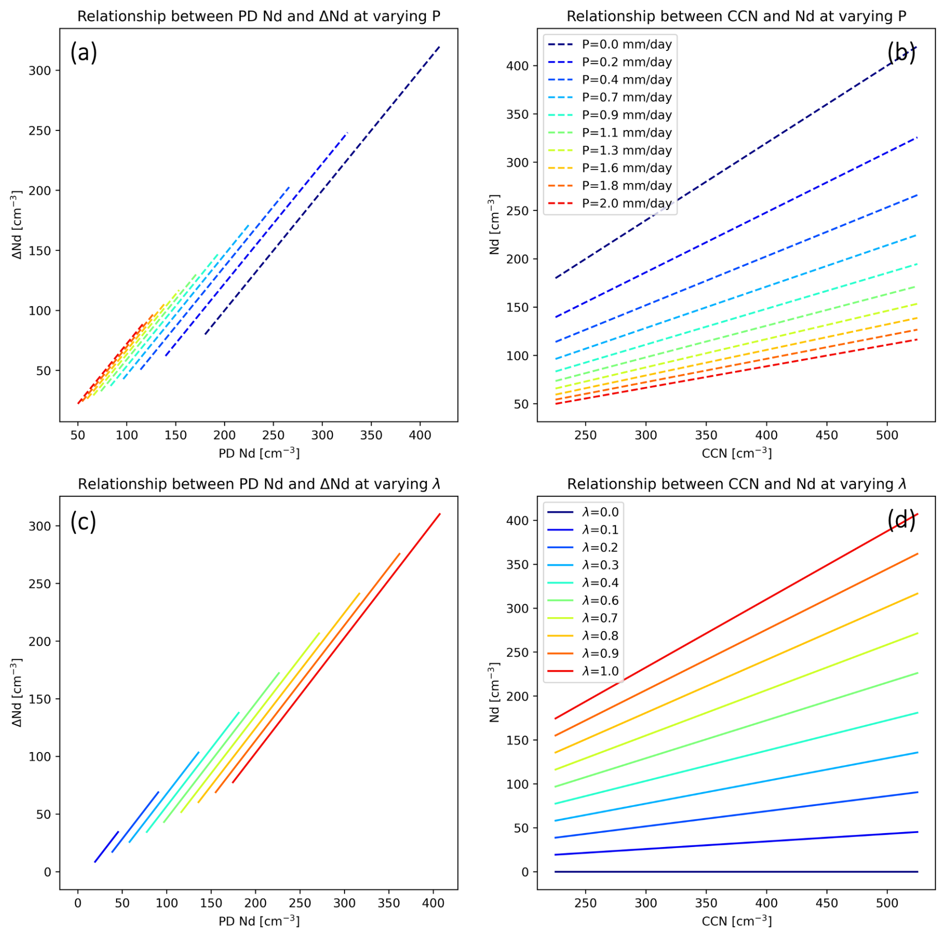
Figure 6 Idealized relationships based on the source-sink model of the N_d budget (Eq. 8 in Wood et al. (2012) with modifications). (a) ΔN_{d, PD-PI} versus PD N_d based on Eqs. (11) and (9) at varying precipitation rate P. P is set to vary from 0 to 2 mm d⁻¹ in 10 equal increments. The varying P is within the observational range in Wood et al. (2012). CCN is set to 125 cm⁻³ as a background CCN from natural source. ΔCCN is set to be varying between 100 to 400 cm⁻³ with 20 equal increments. k_remo is set to 0.8. (b) N_d versus CCN at varying precipitation rate P with the same model setup as (a). (c) ΔN_{d, PD-PI} versus PD N_d at varying CCN scale factor λ. Precipitation rate P is set to 0.2 mm d⁻¹. (d) N_d versus CCN at varying λ with the same model setup as (c).

In this idealized set up, the CCN source (λ⋅CCN) and precipitation sink (k_remo⋅P) are set to be the same between PI and PD. This is a reasonable assumption for CAM6 PPE as its parameter setup is the same in the paired PI and PD simulations. The only difference between PI and PD is the amount of CCN. Therefore, we can write N_d budget model in PI and PD as

$$\begin{array}{}\text{(10)}& {\displaystyle }{N}_{\text{d, PI}}={\displaystyle \frac{\mathit{\lambda }\cdot \mathrm{CCN}}{\mathrm{1}+k_{\mathrm{remo}}\cdot P_{\mathrm{CB}}}}\text{(11)}& {\displaystyle }{N}_{\text{d, PD}}={\displaystyle \frac{\mathit{\lambda }\cdot (\mathrm{CCN}+\mathrm{\Delta }\mathrm{CCN})}{\mathrm{1}+k_{\mathrm{remo}}\cdot P_{\mathrm{CB}}}}\end{array}$$

where ΔCCN in Eq. (11) stands for CCN from anthropogenic aerosol emissions. Equations (10) and (11) allow for a simplified representation of the underlying physical processes driving N_d budget in PI and PD. ΔN_{d, PD-PI} can be calculated by taking the difference between Eqs. (11) and (10)

$$\begin{array}{}\text{(12)}& \mathrm{\Delta }{N}_{\text{d, PD-PI}}={\displaystyle \frac{\mathit{\lambda }\cdot \mathrm{\Delta }\mathrm{CCN}}{\mathrm{1}+k_{\mathrm{remo}}\cdot P_{\mathrm{CB}}}}\end{array}$$

We evaluate the relationship between ΔN_{d, PD-PI} and PD N_d, CCN and N_d using the budget models. We calculate the ΔN_{d, PD-PI} and PD N_d in response to a anthropogenic perturbation of +ΔCCN at varying precipitation rate P_CB and CCN scale factor λ. With this simplified set up, ΔN_{d, PD-PI} and PDN_d, CCN and N_d are positively correlated (Fig. 6), consistent with the CAM6 PPE (Figs. 2, 4). At larger precipitation rate P, more CCN is needed to activate to form the same amount of N_d (Fig. 6b). This leads to an overall lower N_d and N_d change due to aerosols at high precipitation rate (Fig. 6a). With more CCN amount (or larger λ), there is a higher N_d and N_d change due to aerosols (Fig. 6c, d). These results suggest that the positive correlations in CAM6 PPE members are driven by sink from precipitation scavenging and source from CCN as depicted in the idealized model.

Understanding the positive relationships in CAM6 PPE we can use PD observations of N_d to constrain unobservable quantities such as perturbations in N_d due to anthropogenic aerosols. To constrain global-mean quantities, we use observations of N_d from SOCRATES campaign as the variance in global oceanic-mean N_d is largely explained by SOCRATES campaign-mean N_d (Fig. 5). In addition to PD N_d observations, we use the observed aerosol concentration from UHSAS100 from SOCRATES as a proxy of CCN to provide an additional constraints on ΔN_{d, PD-PI} as the parameter spaces of the PPE have been shown to be constrained by CCN in Sect. 3.2 (Fig. 3a). Precipitation processes are constrained by both observations of CCN and N_d as discussed in Sect. 3.2. Inspired by this, we wanted to examine the effects of cloud base precipitation on the constraints on ΔN_{d, PD-PI} . However, we found it difficult to make a direct comparison between CAM6 and cloud radar–lidar–retrieved precipitation rates at cloud base. Therefore, our constraints on ΔN_{d, PD-PI} focus on observations of CCN and N_d. Nonetheless, we provide an illustration of what the constraints would behave if observed precipitation rates were used, based on idealized sensitivity tests discussed in Sect. 3.3.3.

3.3.3 Constraints from CCN and N_d measurements

Before going into the constraints, we first examine the aerosol activation across the PPE members with different parameterizations. Campaign-mean CCN and N_d are positively correlated across PPE ensembles (Fig. 7a), consistent with the CCN-N_d relationship across flight composite in individual models (Fig. 2) and the idealized model (Fig. 6a, c).

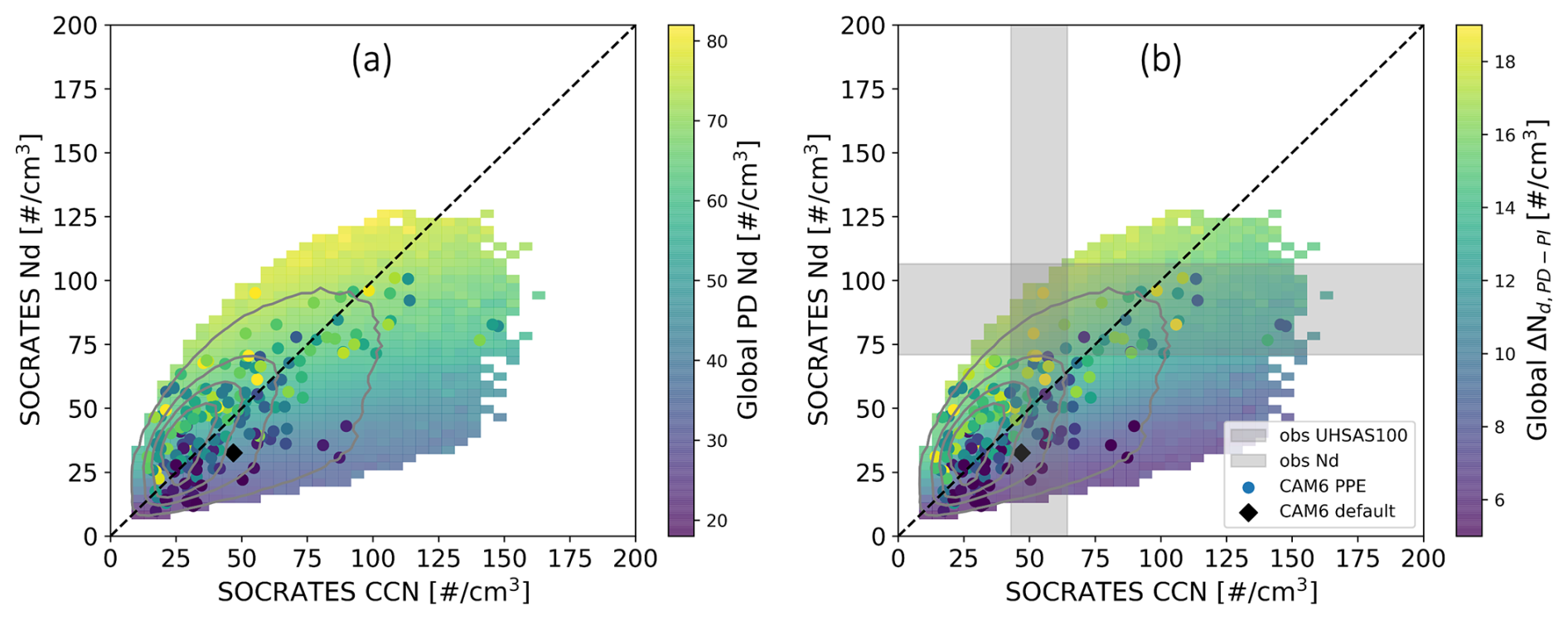
Figure 7 (a) SOCRATES campaign-mean N_d versus campaign-mean CCN and colored by present-day N_d from the CAM6 PPE members (color dots) and 1M emulations from the PPE (color shading). Emulate density is shown in solid contours. (b) The same with (a) but colored by ΔN_{d, PD-PI}. The color shading shows 2D bin-averaged values of (a) global mean N_d and (b) ΔN_{d, PD-PI}, computed using 60×60 bins in SOCRATES CCN and SOCRATES Nd space. This smoothing highlights large-scale patterns while excluding sparsely sampled regions. Colored points show individual PPE members without averaging. Observational SOCRATES campaign-mean CCN (i.e., UHSAS100) and N_d from SOCRATES in-situ measurements is shown as the gray shaded bars with an uncertainty of ±20 % from the campaign-mean.

Understanding emergent relationships is essential in constraining unobservable quantities (Klein and Hall, 2015). With the idealized N_d budget model (Fig. 6), we have understood how the physical processes (i.e., source of N_d from CCN; sink of N_d from precipitation scavenging) are related to the correlations between variables across the CAM6 PPE (Figs. 2, 4). Next, we use airborne observations of CCN and N_d to rule out implausible model variants out of the 1 million variants emulated from the CAM6 PPE (Fig. 7b) following the implausibility metric (Eq. 5). The prior 2.5–97.5th percentile range of ΔN_{d, PD-PI} is 3.6 to 19.8 cm⁻³. Based on the implausibility metric (Eq. 5), observations of CCN have no effect on the constraints on ΔN_{d, PD-PI}. Using the same implausibility metric, observations of N_d over SOCRATES constrains the range of ΔN_{d, PD-PI} to be 6.1 to 20.4 cm⁻³ at the 2.5–97.5th percentile, equivalent to 12 % reduction in range and the median increases by 16 % (Fig. 8a). The constraints on ΔN_{d, PD-PI} are also consistent with the results in Song et al. (2024) that utilizes hemispheric contrast of N_d as a proxy to ΔN_{d, PD-PI} using observations of remote sensing from MODIS, indicating the consistencies between measurements of N_d from different observing techniques.

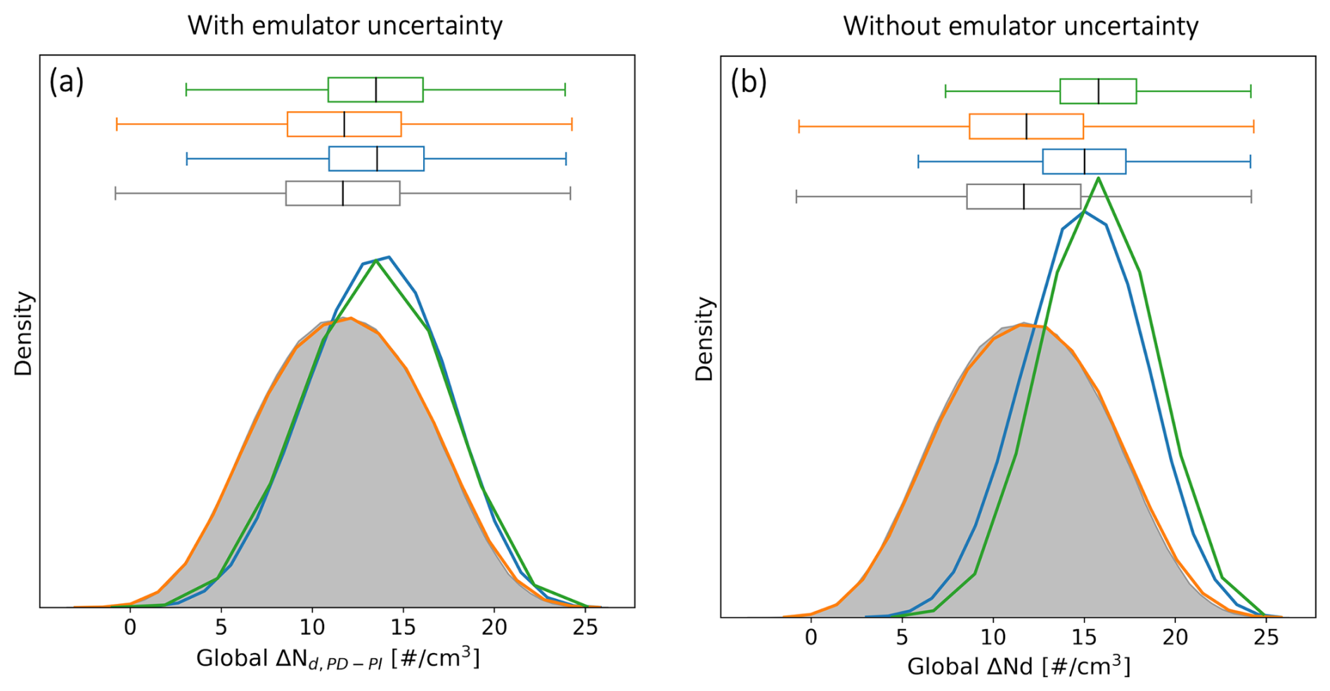
Figure 8 The distribution of emulated ΔN_{d, PD-PI} prior (grey shading), and observationally-constrained posterior from SOCRATES observed CCN only (orange), N_d only (blue), and CCN and N_d (green). (a) With emulator uncertainty. (b) without emulator uncertainty.

In this study, the emulator predictions are based on emulator mean predictions (i.e., M in Eq. 4) and emulator uncertainties (i.e., Error(M) in Eq. 4). Although the emulator mean predictions are overall good, the emulator uncertainty created for CAM6 PPE outputs are relatively large (Fig. S2). This may have a huge impact on the model-observation comparison process (Fig. S3, Eq. 4). We therefore examine the constraints on ΔN_{d, PD-PI} without the effects of emulator uncertainties (i.e., set Error(M) = 0 by setting the number of variance to 0 (i.e., $\mathrm{0}\times \sqrt{\mathrm{Var}\left(M\right)}$) in Eq. 5) to check whether this change significantly affects our constraints. The implausibility metric in this case follows

$$\begin{array}{}\text{(13)}& I\left(x\right)={\displaystyle \frac{|M-O|}{|O\times \mathrm{20}\mathit{\%}|}}>\mathrm{1}\end{array}$$

Consistencies are found in the observational constraints on ΔN_{d, PD-PI} under conditions both with and without emulator uncertainties. Observations of CCN have no effect on the constraints under both conditions (Fig. 8), suggesting that the zero constraint from CCN is not a result of large emulator uncertainties. Instead, the near zero constraint on ΔN_{d, PD-PI} from CCN might be because the CCN provides less information about the number of cloud droplets that can form through aerosol activation compared to direct measurements of cloud droplet numbers. Although CCN number concentration at a given supersaturation accounts for a certain level of chemical composition of aerosols (i.e., hygroscopicity and size), environmental conditions, which is critical for their activation to cloud droplets, is less known. The observational constraints on ΔN_{d, PD-PI} from SOCRATES N_d are consistent in both conditions in terms of the positive shift in the likely range of ΔN_{d, PD-PI}. Observations of N_d narrow the ΔN_{d, PD-PI} range more efficiently under the condition without emulator uncertainties than under the condition with emulator uncertainties. The reduction in range of ΔN_{d, PD-PI} is 21 % and the increase in the median is 28 % when calculated without emulator uncertainties (Fig. 8b).

Observations of CCN and N_d consistently constrain aerosol and precipitation processes as we discussed in Sect. 3.2 so we examined their joint effects on ΔN_{d, PD-PI} in Fig. 8. We found great improvement on the N_d constraint when including the effects of CCN, assuming no emulator uncertainty (Fig. 8b). The ΔN_{d, PD-PI} range is narrowed down by 27 % and the median shifts from 11.7 to 15.5 cm⁻³ (i.e., 35 % increase in median). The result suggests that the direction (e.g., positive or negative shift) of the constraint on ΔN_{d, PD-PI} is not sensitive to emulator uncertainty, while the strength of constraints is sensitive to emulator uncertainty.

Precipitation scavenging works as a sink for both CCN and N_d (Fig. 6a, b), suggesting the strong potential of using precipitation rate as an observational constraints on ΔN_{d, PD-PI}. We found it is difficult to make apples-to-apples comparison between CAM6 and cloud radar-lidar retrieved precipitation rate at cloud base. Therefore, we do not use observed precipitation rates in this study. Instead, we examine what the constraints on ΔN_{d, PD-PI} would respond under two hypothetical campaign-mean surface precipitation rate constraints, used as idealized sensitivity tests. The results suggest that surface precipitation rate has no constraint on ΔN_{d, PD-PI} (Fig. S8). The zero constraint might be due to surface precipitation rate is less informative than cloud base precipitation rate on the N_d budget due to the evaporation during descent. Another possible explanation is that while the precipitation sink explains a lot of variance from flight to flight (Kang et al., 2022), it doesn't vary as dramatically between ensemble member representations of the entirety of the campaign mean because it is strongly controlled by the amount of water vapor and circulation. Overall, we believe further development of instrument simulators for simulating cloud base precipitation rate for global models is needed to improve our ability to leverage airborne cloud base precipitation rate to constrain global behavior.

As discussed in Sect. 2.4, using UHSAS100 as a proxy to CCN at 0.2 % (CCN02) supersaturation may underestimate the observed CCN02. We conduct a sensitivity test on the constraints on ΔN_d,PD-PI by increasing the observed CCN by 8 % to 40 %, based on the 25th to 75th percentile range of the CCN02 : UHSAS100 ratio shown in Fig. S2a of McCoy et al. (2021). The results suggest that increasing the observed CCN does not significantly affect the constraint on ΔN_{d, PD-PI} (Fig. S9).

3.4 Sensitivity tests on the observationally plausible ΔN_d

The uncertainty associated with airborne measurements of aerosol and cloud microphysics is difficult to define as a fixed value because it depends on multiple sources of uncertainties such as: sampling error due to limited spatial and temporal coverage of flight tracks, variability in flight patterns (e.g., altitude, and positioning relative to cloud features), instrument noise due to environmental variability (e..g., turbulence, wind shear). Therefore, assuming a fixed observation uncertainty of ±20 % for airborne measurements in Sect. 3.3.3 is just a to provide a baseline amount of uncertainty.

In this section, we perform sensitivity tests on the observationally plausible ΔN_{d, PD-PI} by the varying observational uncertainty under conditions of with emulator uncertainty (i.e., Error(M) = $\pm \mathrm{1.96}\times \sqrt{\mathrm{Var}\left(M\right)}$ in Eq. 5) and without emulator uncertainty (i.e., Error(M) = $\mathrm{0}\times \sqrt{\mathrm{Var}\left(M\right)}$ in Eq. 5). Systematic uncertainty in the observations is assumed to vary from ±5 % to ±100 % for the campaign-mean. The constraints on ΔN_{d, PD-PI} is calculated as the reduction in the 2.5–97.5 percentile range of ΔN_{d, PD-PI} following Eq. (6).

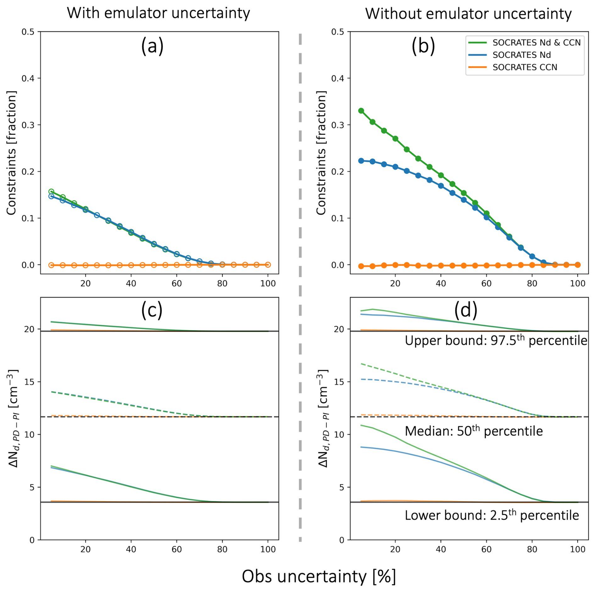
Figure 9 (a) The reduction in the observationally-constrained 2.5–97.5 percentile range of ΔN_{d, PD-PI} relative to the emulation prior range with increasing aircraft measurements uncertainties with emulator uncertainties considered, following the implausibility metric as described in Eq. (5). Observations are from SOCRATES CCN from UHSAS100 (orange), N_d from CDP (blue) and both observations (green). Uncertainty ranges from ±5 % to ±100 % from the campaign-mean with 5 % equal increments. (b) The same (a) but without emulator uncertainty, following the implausibility metric described as Eq. (13). (c) The 2.5th, 50th and 97.5th percentile value of the observationally-constrained ΔN_{d, PD-PI} from SOCRATES CCN (orange), N_d (blue) and both lines of observations (green) as a function of aircraft measurements uncertainties. (d) The same with (c) but without the effects of emulator uncertainty.

Figure 9 shows the constraints on ΔN_{d, PD-PI} by observations of CCN (orange line), N_d (blue line) and combining CCN and N_d (green line). Overall, ΔN_{d, PD-PI} is more tightly constrained without emulator uncertainty (Fig. 9b, d), which makes sense as excluding emulator uncertainties (i.e., Eq. 13) allows more model variants to be excluded during model-observation comparison relative to Eq. (5). The constraints on ΔN_{d, PD-PI} under two conditions (i.e., with and without emulator uncertainty) both have a positive shift in the 2.5–97.5 percentile range (Fig. 9c, d), suggesting the constraints are not a result of noise from emulator uncertainties.

Consistent with Fig. 7, observations of CCN provide nearly no constraint on ΔN_{d, PD-PI} regardless of the uncertainty in CCN (Fig. 9: orange line). With increasing uncertainties from airborne measurements of N_d, the plausible range of ΔN_{d, PD-PI} is less constrained under both conditions of with and without emulator uncertainty (Fig. 9: blue line). The weakened constraints on ΔN_{d, PD-PI} with increasing uncertainties in observations is due to the retention of more model variants as plausible during model-observation comparison process (Fig. S3), thereby exacerbating the equifinality problem (Johnson et al., 2020), for which increasing number of plausible parameter combinations results in broader parameter spaces and thereby reduced constraints on ΔN_{d, PD-PI} (Fig. 9a, b).

The reduction in ranges (constraints) becomes negligible with observation uncertainty of N_d reaching ±75 % under the condition with emulator uncertainty (Fig. 9a). The threshold of observational uncertainty of N_d that can achieve constraints is a bit larger under the condition without emulator uncertainty, which is ±85 % (Fig. 9b), suggesting skillful emulators play an important role in advancing our constraints. Again, we view uncertainty from emulation as an eminently tractable problem compared to developing a better understanding of instrumental systematic uncertainty. Improving emulator uncertainty can be achieved by creating PPEs that can be easily emulated through a more careful selection of perturbed parameters and an increased amount of training data.

Another key insight from Fig. 9 is that the improvement in constraint when both N_d and CCN are considered emerges at low observational uncertainties for both measurements (Fig. 9a, b: green line is above the blue). The improved constraint is also found in Regayre et al. (2023) that adding the number of constraint variables with no structural inadequacies improve the constraints on aerosol forcing when their constraints are consistent across multiple observation types. In our work, although the constraints on ΔN_{d, PD-PI} by observations of CCN is minimal, the constraints on parameter spaces by airborne observations of CCN and N_d are consistent (Fig. 3), resulting in the improved constraints on ΔN_{d, PD-PI}. The improvement of the constraints on ΔN_{d, PD-PI} only happens with small uncertainties associated with airborne measurements (Fig. 9a, b: green line), highlights the importance of accurate airborne measurements of aerosol and cloud properties on constraining ΔN_{d, PD-PI}.

4 Conclusions

We use observations of aerosol (i.e. CCN) and cloud properties (i.e. N_d) from airborne in-situ measurements taken during SOCRATES (the Southern Ocean Clouds, Radiation, Aerosol Transport Study, Fig. 1) to constrain model parameters related to aerosol-cloud interactions. To systematically examine constraints on parameterized processes, we used a PPE that varies 45 parameters related to aerosol-cloud interactions. While a large number of ensemble members (i.e., 262) were integrated across 45-dimensional parameter space, this sampling was still very sparse in an absolute sense. To better map this space, we trained statistical emulators (Fig. S2) to create a set of 1 million model variants. Each model variant was compared against observations and are retained if its implausibility is less than 1 based on the implausibility metric (Fig. S3, Eq. 4). Our constraint on processes in this framework (Figs. 2,  3) resulted in a constraint on the anthropogenic perturbation to N_d (ΔN_{d, PD-PI}) (Fig. 8).

Airborne observations of CCN and N_d over SOCRATES both constrain parameter spaces related to aerosol emission and precipitation processes (Fig. 3), providing insights on developing in-situ instruments targeting these processes to better constrain cloud properties. Observations of N_d are more effective than CCN at constraining parameter space (Fig. 3a, b).

With constrained parameter space with observations of CCN and N_d (Sect. 3.2), we examine the likely range of ΔN_{d, PD-PI} at the constrained parameter space. One key result is that observations of CCN alone have minimal constraint on ΔN_{d, PD-PI}, but the constraint from observations of N_d is strong (Fig. 8). This is sensible because aerosol concentrations from UHSAS100 give information about the aerosol population, but they do not directly inform the activation of aerosols into droplets.

To explain why the constraints work when using observations of N_d, we use idealized sink-source models of N_d (Eqs. 11, 10). Previous work identifies the precipitation sink of droplets as a key driver of N_d variability (Kang et al., 2022; Wood et al., 2012; McCoy et al., 2020). We extended these budget models to anthropogenic perturbations to N_d (Fig. 6), and used the result to understand relationships emergent from the CAM6 PPE (Figs. 2, 4, 7). Within the N_d budget model framework, we identified both the precipitation sink and how CCN form droplets as important in controlling the positive correlation between CCN and N_d (Fig. 6b, d), the positive correlation between present day (PD) N_d and ΔN_{d, PD-PI} in CAM6 PPE (Fig. 6a, c).

Understanding the emergent behaviors from the CAM6 PPE (Fig. 4), we next note that the amount of campaign-mean N_d over SOCRATES is a good approximate of the global oceanic-mean N_d (Fig. 5). Within this framework, observations of N_d over SOCRATES constrains the amount of global ΔN_{d, PD-PI} due to anthropogenic aerosol influence in the CAM6 PPE, with the strong positive correlation between PD N_d and ΔN_{d, PD-PI} in CAM6 PPE (Fig. 4), which can be explained in the context of N_d sources and sinks (Fig. 6).

We find that the range of parameters associated with precipitation processes that are consistent with observations of CCN and N_d is narrow, suggesting the potential of using precipitation rate as an observational constraints on ΔN_{d, PD-PI}. We examine what the constraints would be like if we know the observed surface precipitation. However, the constraints from two hypothetical surface precipitation is minimal (Fig. S8). We did not include cloud base precipitation rate as a constraint due to the difficulty in comparing the simulated cloud base precipitation from CAM6 PPE with cloud base precipitation retrieved from cloud radar and lidar from SOCRATES. We identify further development of instrument simulators for global models as a useful avenue to improve our ability to leverage airborne data (e.g., cloud base precipitation) to constrain global behavior.

We find the constraints are sensitive to the implausibility setup. Overall, observations of N_d constrain ΔN_{d, PD-PI} to a 12 % reduction in range and a 16 % increase in the median, under the condition of with emulator uncertainty (Fig. 8a). The constraint is improved under condition of no emulator uncertainty, for which the reduction in range of ΔN_{d, PD-PI} is 21 % and the increase in the median is 28 % (Fig. 8b). The results suggest reducing emulator uncertainty is important for improving our constraint. More skillful emulators can be achieved by a careful selection of parameters focusing on key processes affecting ACI, particularly aerosol activation, cloud microphysics, and precipitation process as we discussed earlier in Sect. 3.2. Additionally, this work provides insights in the possible parameters ranges in creating PPEs in the discussion of parameter constraints in Sect. 3.

We examine the sensitivity of the constraints on ΔN_{d, PD-PI} with observational uncertainties (Fig. 9). We find discarding parameter combinations that don't mesh with observed CCN and N_d during SOCRATES yields an improved constraint on ΔN_{d, PD-PI} when we disregard emulator uncertainty and when observational uncertainty decreases (Fig. 9a, b). This highlights the importance of considering systematic uncertainties in observations and continuing to develop our understanding of systematic uncertainty in observations of microphysics as well as designing campaigns that allow for stochastic sampling and more direct comparisons to ESMs.

In future work, incorporating additional in-situ constraints, such as aerosol composition, size distributions, or lidar–radar-retrieved cloud and precipitation properties could further narrow the range of plausible PPE configurations. Alternatively, adding more variables as observational constraints may expose structural model uncertainties if the observations are incompatible with any members of the PPE ensemble (Regayre et al., 2023). Instrument simulators that translate model outputs into observation-like quantities (e.g., cloud-base precipitation rate) will also be essential for consistent comparisons. Moreover, incorporating variables such as ice-nucleating particles or ice crystal concentrations, could extend the PPE framework to mixed-phase regimes. While such extensions are beyond the current scope of this study, which focuses on warm liquid clouds, they represent promising directions for future work. Together, these directions can improve the use of PPEs in constraining aerosol–cloud interactions.