Influence of fire-induced heat and moisture release on pyro-convective cloud dynamics during the Australian New Year’s Event: a study using convection-resolving simulations and satellite data

Understanding pyro-convective clouds is essential. These clouds transport significant quantities of aerosols and gases into the upper atmosphere and therefore influence atmospheric composition, weather, and climate on a global scale. This study investigates the dynamics of pyro-convective clouds during the Australian New Years Event 2019/2020 using convection-resolving simulations that incorporate the effects of sensible heat and moisture released by fires. These effects are modeled through parameterizations using retrievals from the Global Fire Assimilation System (GFAS). The results show that the plume top height remains unchanged when accounting for fire-induced heat and moisture release in regions where convective cells form independently of the fire. In areas with the most intense fires, the sensible heat and moisture release from the fire provide the necessary buoyancy for enabling the formation of pyro-convective clouds. Pyro-convective clouds lift aerosol masses up to altitudes of 12.0 km. During their formation, the plume top height more than doubles, compared with a reference simulation in which such clouds do not develop. Additionally, the plume height increase is, on average, just 0.87 km by fire-induced heat and moisture in cloud-free areas. We demonstrated that sensible heat release is the primary contributor to pyro-convective cloud formation. However, the release of moisture enhances the formation process and increases the lifetime of the pyro-convective cloud. Comparisons with observational data show that the plume's distribution and height are underestimated. However, the simulations align well with observations after a 5–6 h delay, indicating that pyro-convective cells are accurately modeled but occur later in the model than are actually observed.

1 Introduction

Pyrocumulonimbus (pyroCb) clouds emerge from intense wildfires, generating lightning, hail, downdrafts, and tornadoes but minimal precipitation (Fromm et al., 2022). Smoke particles and gases get transported by pyroCb events up to the upper troposphere and lower stratosphere. This affects the global climate by altering atmospheric composition and radiative balance (Fromm et al., 2022). The formation of pyroCbs is highly sensitive to atmospheric stability and fire intensity, which can change throughout the day (Luderer et al., 2006). The general assumption is that, while a stable atmosphere typically suppresses vertical air movement, limiting wildfire plume heights and convection in the morning, as the day warms, the atmosphere becomes more unstable. This instability allows for higher plume heights and more vigorous pyro-convection, potentially forming pyroCbs (Luo et al., 2022). Wildfires follow a diurnal cycle as well: cooler morning temperatures and higher humidity reduce fire intensity and spread. As temperatures rise and humidity drops during the day, fire intensity and spread increase, with stronger winds further enhancing fire spread. In the evening, lower temperatures and higher humidity reduce fire intensity (Andela et al., 2015; Loudermilk et al., 2022). This leads to a majority of pyroCb clouds forming and reaching maturity in the late afternoon (Fromm et al., 2010). However, there are exceptions to this typical diurnal cycle of meteorology and fires. As outlined by Luderer et al. (2006), cold fronts can induce significant temperature drops before sunset, which are substantially greater than the usual diurnal variations experienced in the late afternoon. Furthermore, recent studies have shown an increase in nighttime fire activity, particularly in larger wildfires. This increase is attributed to warmer and drier nighttime conditions, which can sustain fire activity throughout the night (Balch et al., 2022).

Although pyroCb clouds are a common and well-studied phenomenon, much remains unknown about their behavior, energetics, history, and impact on the Earth–atmosphere system (Fromm et al., 2022). This challenges the reliable simulation of pyro-convective clouds. Failure to accurately simulate these clouds is accompanied by an incorrect calculation of plume height, as the formation mechanism of pyro-convective clouds releases latent heat, which generates additional buoyancy. The effect of fire on meteorological variables and, consequently, pyro-convective cloud formation is often not included in global and regional models. This omission leads to errors in the injection height of gases and particles, subsequently affecting their transport. To parameterize these processes accurately, a comprehensive understanding of the interplay between fire-induced buoyancy, latent heat release, and atmospheric stability is essential.

Significant progress has been made in understanding these phenomena. Numerous studies with coupled fire–atmosphere models have addressed the uncertainties of fire–atmosphere interactions by accounting for fire dynamics. For example, research by Clark and Packham (1996) and Clark et al. (2004) employs fine grid resolutions ranging from 4 to 120 m. These studies primarily focus on wind changes induced by the fire and how these changes impact the fire itself. Despite these advancements, further research is needed to fully comprehend the complexities of pyro-convective transport and its broader implications. Kochanski et al. (2013) and Kiefer et al. (2010, 2016, 2018) use nested fire–atmosphere models in coarser grid resolutions to simulate meso-scale effects. However, it remains partially unclear how fires influence cloud and plume dynamics, and consequently long range transport, due to the spatial limitations of the simulation domains.

The study by Trentmann et al. (2006) focuses on pyro-convective clouds and explicitly simulates plume rise. It concludes that sensible heat release initiates convection, while latent heat release from condensation and freezing dominates the total energy budget. The study finds that the available moisture is primarily entrained, with negligible contribution from fire-released moisture. Luderer et al. (2006) further investigate these findings through sensitivity studies, concluding that meteorological conditions play a dominant role in pyro-convection. They find that the emission of water vapor is less important for the emission height than sensible heat release but enhances the aerosol amount transported to the tropopause level. Additionally, they find that the dynamics and evolution of pyroCbs are weakly sensitive to aerosols acting as cloud condensation nuclei (CCN). This is in contrast to studies by Reutter et al. (2014) and Chang et al. (2015), who highlight the significant role of aerosols in influencing pyro-convective cloud dynamics and microphysics. They underscore the importance of including detailed aerosol–cloud interactions in high-resolution atmospheric models to accurately simulate cloud formation and precipitation processes. Lee et al. (2020) further report that the aerosol effect on pyroCb development is more significant in cases of weak-intensity fires, compared with strong-intensity fires. Findings by Kablick III et al. (2018) highlight the significant impact of surface heat flux on pyroCb properties and suggest that pyroCb events could influence lower stratospheric water vapor. All this outlines the complexity and variety of processes that influence pyro-convective cloud formation. Understanding these dynamics is crucial, not only from a cloud microphysical perspective but also for aerosol plume development, as plume height is a key factor in plume transport (Val Martin et al., 2006). Knowledge of the injection height is essential for accurately parameterizing injection heights in global transport models and, therefore, for reliably calculating transport.

The smoke emission and dispersion are influenced by the composition, structure, and condition of the fuel, as well as the weather and topography. Consequently, each fire is unique, making it challenging to accurately capture this variability in simulations. Additionally, the limited in situ measurements and the significant spatial and temporal variability of biomass burning make it challenging to accurately monitor fire characteristics and retrieve necessary inputs for plume-resolving simulations. To overcome the dependence on individual measurements, we developed a method to parameterize sensible heat and moisture release in models using satellite retrievals from the Global Fire Assimilation System (GFAS), which are based on MODIS observations (Kaiser et al., 2012; Copernicus Atmosphere Monitoring Service, 2021). As the name suggests, GFAS provides a global dataset that delivers information about a fire within 24 h of its occurrence. We tested our developments by simulating part of the Australian New Year's Event (ANY) event in a limited area mode and resolving convection. ANY refers to an extreme outbreak of pyroCbs that occurred in south-east Australia around New Year 2019/2020 (Peterson et al., 2021). There were 38 pyroCbs, reported between the 29 December 2019 and 4 January 2020, divided into 18 sub-events (Peterson et al., 2021). This pyroCb activity resulted in an emission from approximately 1.0 Tg of biomass burning aerosol into the lower stratosphere and had an impact on the atmospheric dynamics, chemistry, and radiation budget (Peterson et al., 2021).

The extreme fire weather conditions occurred when a cold front passed through the region on 30 December. Additionally, a negatively tilted upper-tropospheric trough, interactions with topography, the presence of low-level overnight jets, and horizontal boundary layer rolls further exacerbated the situation. In combination, these factors created conditions for rapid fire spread and intense pyroCb activity, especially during the night.

In this study, convection-resolving simulations are performed and analyzed to determine if the atmospheric impact of these intense fires is captured and to answer the following research questions.

1. How do fire-induced heat and moisture release affect plume and cloud formation under unstable atmospheric conditions?

2. What are the discrepancies between simulated and observed plume top heights and spreads and how suitable are satellite-constrained fire data from GFAS for accurately simulating pyro-convective clouds?

In the following section, the model system, the developed parameterizations, and the simulation setup of the performed experiment are described. Then, the results are analyzed and discussed, and the conclusions are presented.

2 Methods and materials

2.1 The ICON–ART modeling system

The model used for this work is the Icosahedral Nonhydrostatic (ICON) numerical weather and climate model. ICON solves the full three-dimensional nonhydrostatic and compressible Navier–Stokes equations on an icosahedral grid (Zängl et al., 2015). The ICON model is able to perform seamless simulations of various processes, from local to global scales (Heinze et al., 2017; Giorgetta et al., 2018).

Furthermore, the ART (Aerosol and Reactive Trace Gases) module is enabled. It includes the emission, transport, physicochemical transformation, and removal of aerosols and trace gases (Rieger et al., 2015). Detailed descriptions are given in Rieger et al. (2015), Schröter et al. (2018), and Muser et al. (2020).

2.2 Parameterization of heat and moisture release and aerosol emission

A parameterization for sensible heat and moisture release and aerosol emission based on satellite retrievals from GFAS was developed. GFAS uses the fire radiative power (FRP) from NASA’s MOD14 product. MOD14 includes thermal radiation observations (λ≈ 3.9–11 µm) from the polar-orbiting satellites MODIS Aqua and Terra (Giglio, 2007; Justice et al., 2011). For the parameterization of the sensible heat release, the FRP is used. The GFAS dataset provides the FRP and, therefore, the radiative fraction of total heat release. The FRP is multiplied by a factor of 10 to retrieve the total energy released by the fire, as proposed by Val Martin et al. (2012) and further applied in Ke et al. (2021). A factor of 0.55 is applied to convert the total energy to convective energy. This factor is taken from Freitas et al. (2006), following McCarter and Broido (1965), and is similar to the convective fractions of 0.518 and 0.52 proposed in Freeborn et al. (2008) and Morandini et al. (2013), respectively. The FRP is weighted with the diurnal cycle function proposed by Andela et al. (2015) and applied by Walter et al. (2016) in COSMO–ART to account for peak fire intensity in early afternoons, given as

$$\begin{array}{}\text{(1)}& d\left(t_{\mathrm{1}}\right)=\mathit{\omega }+(\mathrm{1}-\mathit{\omega }){\displaystyle \frac{\mathrm{1}}{\mathit{\sigma }\sqrt{\mathrm{2}\mathit{\pi }}}}\exp \left(-{\displaystyle \frac{\mathrm{1}}{\mathrm{2}}}{\left({\displaystyle \frac{t_{\mathrm{1}}-t_{\mathrm{0}}}{\mathit{\sigma }}}\right)}^{\mathrm{2}}\right)\end{array}$$

and visualized in the Appendix. Here ω is a weighting, which is set according to the vegetation type in the respective grid cell: ω is 0.039 for tropical forests, 0.018 for savannas, and 0.003 for grassland. In addition, t₁ is the local solar time, t₀ is the expected value of maximum emission, set to 12.5, and σ is the standard deviation, set to 2.5. The heat release is implemented as sensible heat flux from the surface to the atmosphere. This leads to a sensible heat release by the fire, sh_fire, of

$$\begin{array}{}\text{(2)}& {\mathrm{sh}}_{\mathrm{fire}}=\mathrm{FRP}\times \mathrm{5.5}\times d,\end{array}$$

where FRP and sh_fire both have units of watts per square meter.

The implementation of the moisture release parameterization includes combustion moisture, with an emission ratio of 0.75 H₂O $/$ (CO + CO₂) (Parmar et al., 2008). The CO and CO₂ emission fluxes from GFAS are scaled and emitted in the ICON specific humidity tracer. Additionally, fuel moisture is emitted. The fuel moisture is divided into dead and live components and follows thresholds from Nolan et al. (2016) and Deb et al. (2020). Assuming 30 % dead and 70 % live fuel, the approximate fuel moisture is 75.42 %, multiplied by the GFAS combustion rate. The live-to-dead fuel ratio is taken from Hines et al. (2010). The moisture emission flux by the fire, qv_fire (kg m⁻² s⁻¹), is calculated according to

$$\begin{array}{}\text{(3)}& {\mathrm{qv}}_{\mathrm{fire}}=\left(\mathrm{0.75}\times (m_{\mathrm{CO}}+m_{{\mathrm{CO}}_{\mathrm{2}}})+\mathrm{0.7542}\times m_{\mathrm{load}}\right)\times d,\end{array}$$

using mass fluxes of CO (m_CO) and CO₂ ($m_{{\mathrm{CO}}_{\mathrm{2}}}$) and the combustion rate m_load. All three have the unit kg m⁻² s⁻¹. The moisture emission flux is weighted with a diurnal cycle function d. Next, the moisture emission flux is converted to the mass mixing ratio and added to the specific humidity tracer at the lowest model level.

For the aerosol emission, the GFAS black carbon m_BC and organic carbon m_OC fluxes are combined, weighted by the diurnal cycle function, as

$$\begin{array}{}\text{(4)}& e_{\mathrm{fire}}=(m_{\mathrm{OC}}+m_{\mathrm{OC}})\times d.\end{array}$$

The particles are emitted into the lowermost model level, analogous to the moisture emission. The GFAS daily mean mass fluxes, m_OC and m_OC, are provided in kg m⁻² s⁻¹; therefore, e_fire has the unit kg m⁻² s⁻¹.

2.3 Model configuration

For this work, a limited area mode simulation is performed. The area of the domain is shown in Fig. 1, in the black box, and is approximately 340 km in length (north–south) and 230 km in width (east–west). Prior to the experimental simulations, a global simulation with a grid spacing of 13 km is conducted to obtain the input data for the boundary conditions. This global simulation is initialized using the German Weather Service (DWD) analysis product and does not account for fire impacts on the meteorological variables. The experimental simulations are also initialized with the DWD analysis product and meteorological variables of the boundary conditions are read every 30 min. The grid spacing is 0.6 km and there are 125 vertical levels from the surface to a maximum height of 30 km. The level thickness increases from, on average, 95 m in the lowermost level to 550 m at the top. Due to the high spatial resolution, the schemes for convection, subgrid-scale orographic effects (blocking and gravity wave drag), and nonorographic gravity wave drag are de-activated (Dipankar et al., 2015). However, this study does not consider aerosol–cloud and aerosol–radiation interactions. For cloud microscopical processes, a single-moment scheme is used that predicts the categories of cloud water, rain water, cloud ice, and snow. The simulations start on the 29 December at 18:00 UTC, which corresponds to 05:00 on the 30 December in Australian Eastern Daylight Time (AEDT), and last for 20 h. The fire emissions are initialized based on assimilated FRP observations provided by GFAS (NASA LAADS DAAC, 2025). The particle emissions include black and organic carbon, which are emitted in the lowermost model layer. The size distribution of the aerosols is approximated by a log-normal distribution with a median number diameter d_n=70 nm and a standard deviation of σ=2.0. The simulation does not consider atmospheric chemistry, nucleation, or condensation but does consider coagulation.

Three simulation experiments were performed: a reference experiment, termed “REF,” which only accounts for aerosol emission, neglecting heat and moisture release; a second experiment, termed “SH,” where additionally sensible heat released by the fire is accounted for; and a third experiment, termed “SHLH,” where both sensible heat and moisture release are enabled.

The FRP in the experiment domain is shown in Fig. 1. During the simulation, a peak sensible heat release of 2.24 kW m⁻² is reached. The peak fire-induced water vapor flux reaches 1.07 $\times {\mathrm{10}}^{-\mathrm{6}}$ kg m⁻² s⁻¹; assuming that the latent heat of condensation for water is approximately 2257 kJ kg⁻¹, the potential additional latent heat flux can reach a maximum of 0.02 W m⁻².

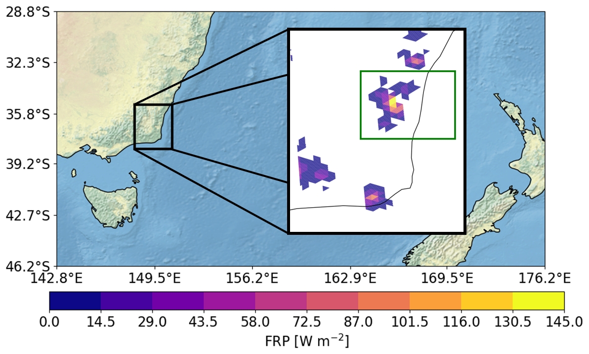
Figure 1 The black box shows the simulation domain and FRP input. The green box indicates the area with the largest FRP, in approximately the center of the domain.

2.4 Height retrievals

The NASA 3D wind retrieval algorithm, as described by Carr et al. (2018, 2019, 2020), is employed to determine the height of plumes and clouds. This algorithm leverages stereo imaging, which utilizes geometric parallax to retrieve feature heights. By integrating data from geostationary (GEO) and low-earth orbit (LEO) satellites, it generates three-dimensional (3D) atmospheric motion vectors (AMVs) through a multi-platform, multi-angle, stereoscopic approach. The term “3D winds” refers to the three-dimensional positioning of horizontal AMVs within the atmosphere. Observing the parallax of a feature from two different vantage points (stereo) provides direct information about its height. For this study, the LEO–GEO retrieval method is utilized. The LEO satellite data come from Terra and Aqua MODIS Level 1B in the blue band (459–479 nm), with a 500 m resolution. The GEO satellite data are from Himawari 8’s blue band (430–480 nm) (Japan Meteorological Agency (JMA) and National Oceanic and Atmospheric Administration (NOAA), 2025). The Advanced Himawari Imager (AHI), operated by the Japan Meteorological Agency, has a 10 min temporal resolution that is used to track feature movement. MODIS data are then used to calculate parallax, determining AMVs and height. A quality flag is used to remove poor retrievals.

2.5 Definitions and analysis methods

In this section, the analysis of plume and cloud heights is conducted. Accordingly, a plume is defined as a grid cell that exceeds an aerosol mass mixing ratio of $\mathrm{5}\times {\mathrm{10}}^{-\mathrm{8}}$ kg m⁻³ and a cloud is defined as a grid cell that exceeds a mass mixing ratio of liquid water content (LWC) + ice water content (IWC) of $\mathrm{5}\times {\mathrm{10}}^{-\mathrm{6}}$ kg m⁻³. Consequently, the top height is the level with the highest altitude exceeding this threshold.

Furthermore, the temporal evolution of the plume top heights for a cloud-free plume, a plume with clouds, and a plume with pyro-convective clouds is analyzed. For this analysis, a threshold of 1 kg m⁻³ is chosen for the plume. By adopting a higher threshold, we ensure that the diagnosed plume top reflects the dynamically relevant upper extent of the convective column, rather than transient or diluted features near the top of the plume. The presence of clouds within the plume is defined via a threshold for the sum of LWC and IWC within a grid cell. The plume is considered cloud-free if the grid cell has a mass mixing ratio of LWC + IWC smaller than $\mathrm{1}\times {\mathrm{10}}^{-\mathrm{32}}$ kg m⁻³. In the plume with clouds case, LWC + IWC within a grid cell must be greater than $\mathrm{1}\times {\mathrm{10}}^{-\mathrm{32}}$ kg m⁻³. The plume with pyro-convective clouds is defined by an increase in aerosol mass mixing ratio of $\mathrm{1}\times {\mathrm{10}}^{-\mathrm{6}}$ kg m⁻³ and an increase in LWC + IWC of $\mathrm{5}\times {\mathrm{10}}^{-\mathrm{8}}$ kg m⁻³ within a grid cell, compared with the REF experiment. Since there is no pyro-convective cloud in the REF experiment, the grid cells corresponding to the SHLH experiments are used. The displayed top heights are the mean values of the 100 highest plume top heights, calculated for each experiment over time.

3 Results

3.1 Comparison of model results and observations

To begin, the simulated plume height is compared with observational data to assess the accuracy of our model. Therefore, the simulated plume top heights are compared with the retrieved top height from the NASA 3D Wind Algorithm. It should be noted that the resolution of the retrieval is approximately 2.2 km, which is coarser than the simulation, with a grid spacing of 600 m. Therefore, the simulation is displayed with a mask that maps the observation points to the closest grid points.

The observations in Fig. 2a show aerosols and clouds above the fires with heights ranging between 5 and 12 km. Because the retrieval is not able to separate clouds from aerosols, the plots display either the plume or the cloud top height. The SHLH experiment, in comparison with the observations, shows smaller elevated areas of the plume and has lower maximum heights. The plume in the north-eastern part of the domain remains below 5 km. Close to the fire areas, cloud heights above 10 km are simulated, but these clouds form independently of the fire, as they are also simulated in REF (Fig. A2 in the Appendix). The time of observation is 5.5 h into the simulation at 10:30 AEDT. This indicates that particles are only emitted for 5.5 h, and fire intensity and emission flux have not peaked, whereas the observations include the background aerosols of fires burning for days and originating from farther away.

Figure 2c and d show the comparison of cloud and plume height retrieval and the SHLH experiment for 30 December 2019 at 14:30 AEDT. The observations in Fig. 2c show plume and cloud heights in the range between 5 and 12 km above the fire; in the south-western part of the domain, heights above 12 km are reached. In the SHLH experiment (Fig. 2d), heights above 10 km are simulated; these result from clouds independent of the fire, as outlined in Fig. A2. The simulation time is 9.5 h and the simulated plumes in the area of the green box are, again, underestimated in the distribution but selectively match the observed top heights.

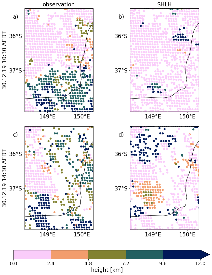
Figure 2 Plume and cloud top heights for (a, b) 30 December 2019 at 10:30 AEDT and (c, d) 30 December 2019 at 14:30 AEDT: (a, c) retrieved from the NASA 3D Wind Algorithm, (b, d) simulated for the SHLH experiment.

To better understand these differences, a thorough understanding of the assumptions made and the underlying processes is necessary. The fire input data remain a major source of uncertainty. The daily mean values provided by GFAS and the assumed generally applicable diurnal cycle are crude approximations. This is illustrated in Fig. 3. Firstly, it is evident that the magnitude of the assumed FRP for the simulation underestimates the FRP observed by MODIS. This is expected, as the assumed FRP for the simulation is based on GFAS, which provides a daily mean value averaged over a 1°×1° grid, compared with the MODIS active fire data at a 1 km resolution. The MODIS data have limited measurements, due to the overpass times; however, they do not show a clear diurnal cycle, as assumed in the parameterization. On the contrary, the measurements indicate high FRP during the night. As mentioned, for this particular event, high nighttime fire activity and pyroCb formation were reported.

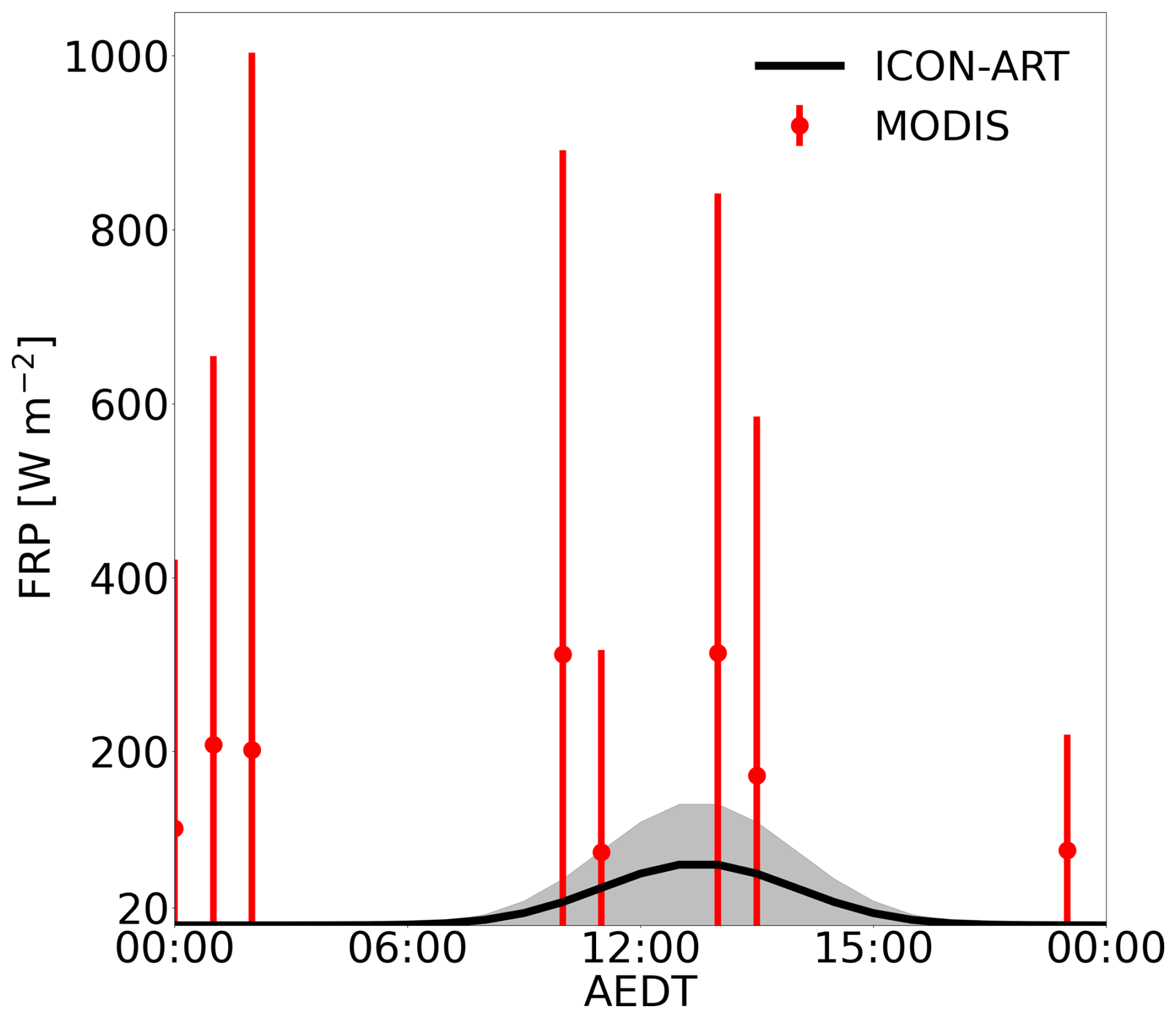
Figure 3 The averaged FRP assumed in the simulations (black line), with the standard deviation in gray. Red dots represent the mean MODIS active FRP (NASA and University of Maryland, 2025) for each hour with measurements during the simulation period, along with the standard deviation.

This leads to a structural limitation in our assumption of fire activity and may contribute to the underestimation of simulated plume height and spread, compared with observations, as the simulation starts in the early morning, probably underestimating fire intensity. While this limitation is acknowledged, the aim of this study is not to achieve an optimized case-specific simulation of the ANY event. Rather, we seek to evaluate how well pyro-convective processes can be represented using a standard model configuration. Therefore, we proceed with the analysis of the experiment. The following section elaborates on the impact of fire-induced heat and moisture release on plume evolution and cloud formation.

3.2 Plume height and cloud formation

First, the impact of both sensible heat and moisture release (SHLH experiment) on plume height and cloud formation is quantified, before the contribution of each individual effect (SH compared with SHLH) is discussed.

Figure 4 displays the temporal evolution of the plume top height in the REF and SHLH experiments. The first row (a–c) displays the temporal evolution of the plume top height in the REF experiments. At 13:00 AEDT, the plume top height peaks in the north-east corner of the domain, with a maximum height of 13.71 km. At 16:00 AEDT, in Fig. 4b, two more plumes rise above 10 km. The elevated plumes are transported south-east/east, as shown in Fig. 4c. The experiments SHLH and REF exhibit notable similarities in distribution and maximum height. The main difference between the experiments is observed in the center of the domain. This area is marked with a green box, as in Fig. 1. In the center of the domain, maximum heights up to 12.8 km are reached for the SHLH experiment, which is a significant increase, compared with the REF experiment, with plume heights remaining below 2.5 km.

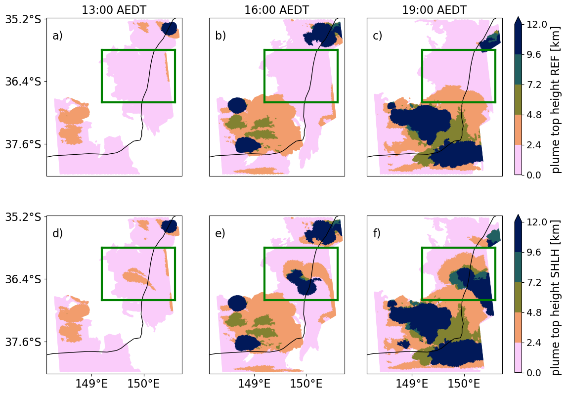
Figure 4 Temporal evolution of plume top height for (a–c) the REF experiment and (d–f) the SHLH experiment: (a, d) 13:00 AEDT, (b, e) 16:00 AEDT, (c, f) 19:00 AEDT. The central part is marked with a green box.

The results for the area within the green box, with the largest emissions, might suggest that a critical sensible heat and moisture release has to be reached for pyro-convective cloud formation. However, the plume top height resulting from these fires is comparable to those originating from the north-eastern and western parts of the domain, where convective clouds form independently of the fire.

Figure 5 displays the temporal evolution of the liquid and ice water paths (LWP and IWP) in the REF experiment (a–c). The values of LWP + IWP in Fig. 5a indicate cloud formation at the northern and western boundaries of the domain. This suggests that clouds form independently of the fire’s effect on meteorological variables, although it is possible to identify individual convective cells that overlap the fire area. The cloud cover moves and spreads from the western boundary to the south-east, resulting in a nearly diagonal cloud formation throughout the domain by 19:00 AEDT. As discussed in the introduction, the ANY event was characterized by a passing cold front that created atmospheric instability and convective clouds; this is captured by the simulation. The second row (d–f) displays the difference in LWP + IWP between the SHLH and REF experiments. Figure 5d shows some cloud formation due to the release of sensible heat and moisture. Within the green box, LWP + IWP starts to increase and, as shown in Fig. 5e, cloud formation increases up to 4.46 kg m⁻². Last, Fig. 5f primarily exhibits noise. Overall, the fire-induced heat and moisture lead to additional cloud formation in some regions with pre-existing clouds, with a negligible influence on the plume top height. The temporal evolution in the region marked with the green box shows a clear increase in cloud water and ice, indicating that convection explains the increase in plume top height in Fig. 4.

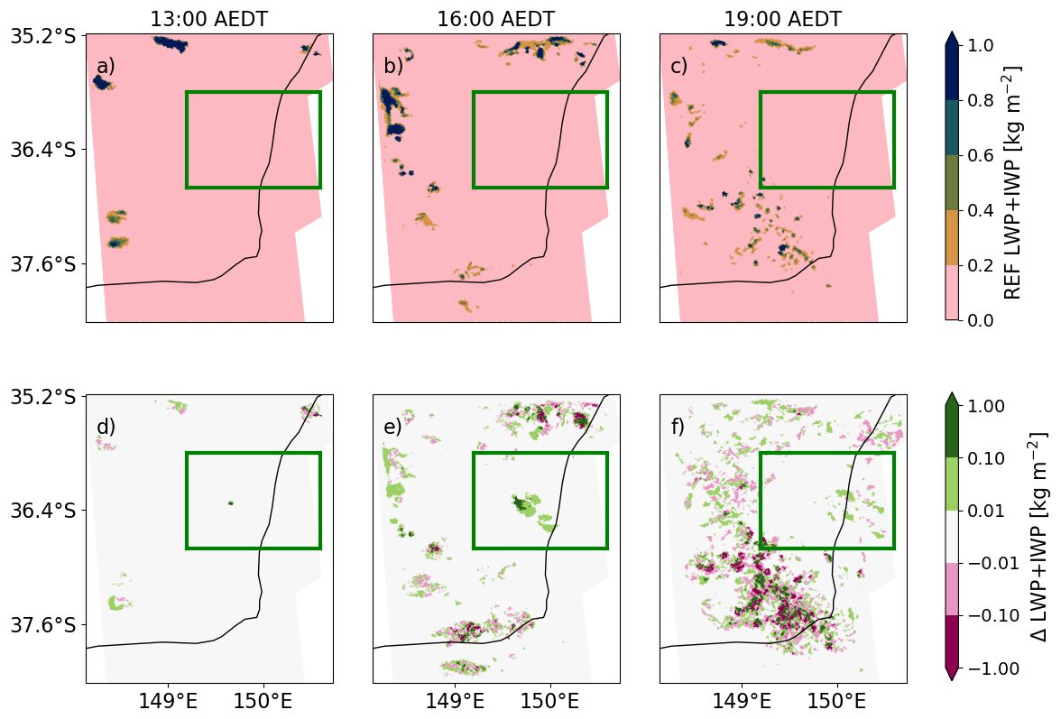
Figure 5 Temporal evolution of LWP + IWP for (a–c) the REF experiment and (d–f) the difference between the REF and SHLH experiments: (a, d) 13:00 AEDT, (b, e) 16:00 AEDT, (c, f) 19:00 AEDT. The central part is marked with a green box.

In the next step, the impact of moisture release on cloud formation is analyzed. The temporal evolution of LWP + IWP in the SH experiment and the difference in LWP + IWP between the SHLH and SH experiments are shown in Fig. 6, structured the same as Fig. 5.

The SH shows remarkable similarities to REF, except in the region of the green box. There, a convective cloud forms, with LWP + IWP values of 5.37 kg m⁻², at 16:00 AEDT and dissipates at 19:00 AEDT. This indicates that fire-induced moisture release is not necessary for the formation of a pyro-convective cloud. The impact of moisture release is highlighted in Fig. 6d–f. The cloudy regions outside the green box predominantly display noise, with the signal intensity increasing over time. Figure 6d shows a small overall increase, with a total increase in LWP + IWP in that area by 10.6 %. The LWP + IWP in Fig. 6e decreases by 10.8 % and that in Fig. 6f only increases by 1.3 %.

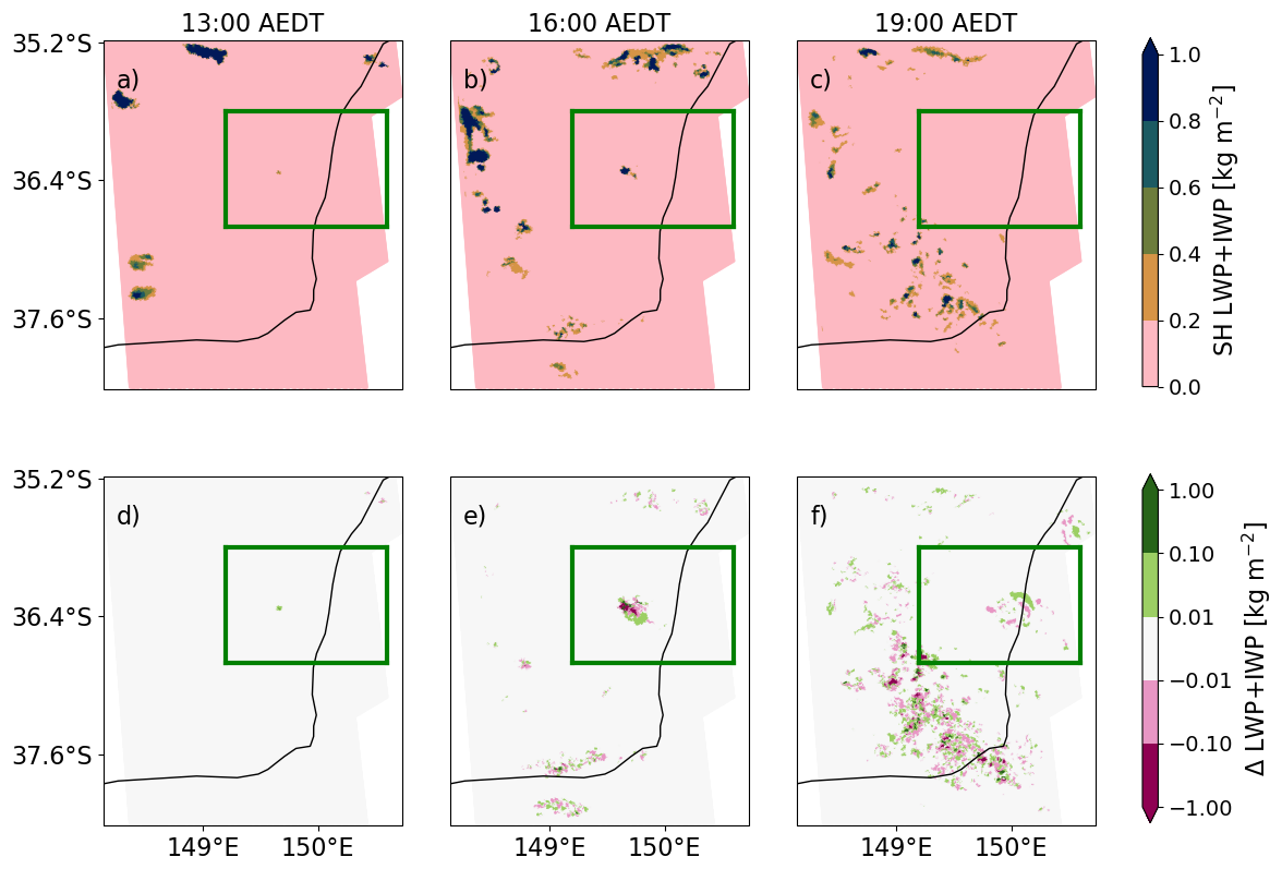
Figure 6 Temporal evolution of LWP + IWP for (a–c) the SH experiment and (d–f) the difference between the SHLH and SH experiments: (a, d) 13:00 AEDT, (b, e) 16:00 AEDT, (c, f) 19:00 AEDT. The central part is marked with a green box.

In Figures 4–6, the impact of fire–atmosphere interaction is most dominant in the area indicated by the green box. To understand this further, we analyze the atmospheric stability. Table 1 shows how the fire–atmosphere interaction impacts surface-based convective inhibition (CIN) and surface-based convective available potential energy (CAPE) in the area marked by the green box (GB) and elsewhere for 16:00 AEDT on the 30 December. The average CIN and CAPE values are calculated within the fire area for the corresponding experiments. The CIN in the REF model indicates that, outside of the area marked by the green box, the atmosphere is less resistant to the initiation of convection. Furthermore, the CAPE values suggest that more energy is available for convection, which can lead to stronger and more vigorous updrafts outside of the area marked by the green box. This is consistent with the formation of convective clouds at the borders of the domain but the absence of clouds within the area marked by the green box. Comparison of the CIN of the REF experiment with the SH and SHLH experiments shows a reduction in CIN by around 35 % outside of the area marked by the green box and by 44 % within the area marked by the green box. This reduction in CIN indicates that the atmosphere is less resistant to the initiation of convection, making it easier for fire-induced updrafts to develop. The CAPE values in the SH and SHLH experiments more than double outside the area marked by the green box and increase by a factor of over 4.8 within the area marked by the green box. Higher CAPE means that more energy is available for convection; this can lead to stronger and more vigorous updrafts. The impact of additional moisture release on CIN is less than 1 %, and the increases in CAPE remain below 1.5 %.

Table 1 Surface-based convective inhibition (CIN) and convective available potential energy (CAPE) in the fire areas outside of the green box and inside the green box (marked GB) for the REF, SH, SHLH experiments on 30 December at 16:00 AEDT. The values are given in joules per kilogram.

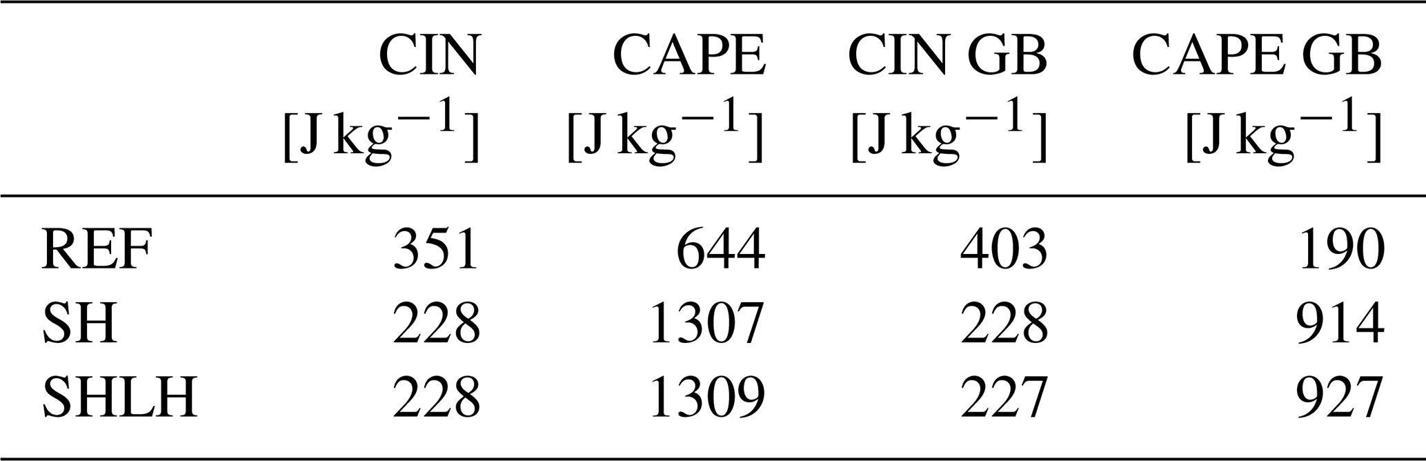
Figure 7 illustrates the temporal evolution of plume height for the cloud-free plume, the cloudy plume, and the plume area with clouds formed through pyro-convection. Figure 7a shows results for the cloud-free plume. It should be noted that, at the beginning of the simulation, the plume is dense and concentrated close to the fires. This means that the number of grid points that mask the plume is initially small but increases as the plume spreads. Therefore, during the first 8 h of the simulation, the number of cloud-free grid points remains below 100. During the day, the number of masked grid points is of the order of 10 000. The diagnosed plume top height remains around 0 in the morning. After 12:00 AEDT, the top height increases for all experiments but then decreases from the evening onward. The evolution of the top height in REF demonstrates the diurnal cycle of the atmosphere, which allows for enhanced vertical movement in the afternoon. The SH and SHLH experiments further emphasize the buoyancy created by the fire, which is also influenced by a diurnal cycle. Comparison of the SH and SHLH experiments reveals that the impact of the buoyancy from the sensible heat is dominant.

Figure 7b displays the evolution of the plume where clouds are also present. This mask includes many more grid points than the no-cloud mask, with grid point numbers of the order of 10⁵. In experiments accounting for fire-induced heat, there is an increase in plume top height of up to 500 m in the morning. A significant increase to around 12.2 km is observed for all experiments around 13:00 AEDT, corresponding to the emergence of the first convective cloud cell, as the atmosphere becomes more unstable throughout the day and fire activity peaks. The impact of moisture release on the plume top height is small, with an average increase of 30 m. The REF experiment further shows a decrease in plume top height at 21:00 AEDT, which can be explained by the lower concentrations in the upper levels that no longer exceed the threshold and the transport of the elevated plume out of the domain.

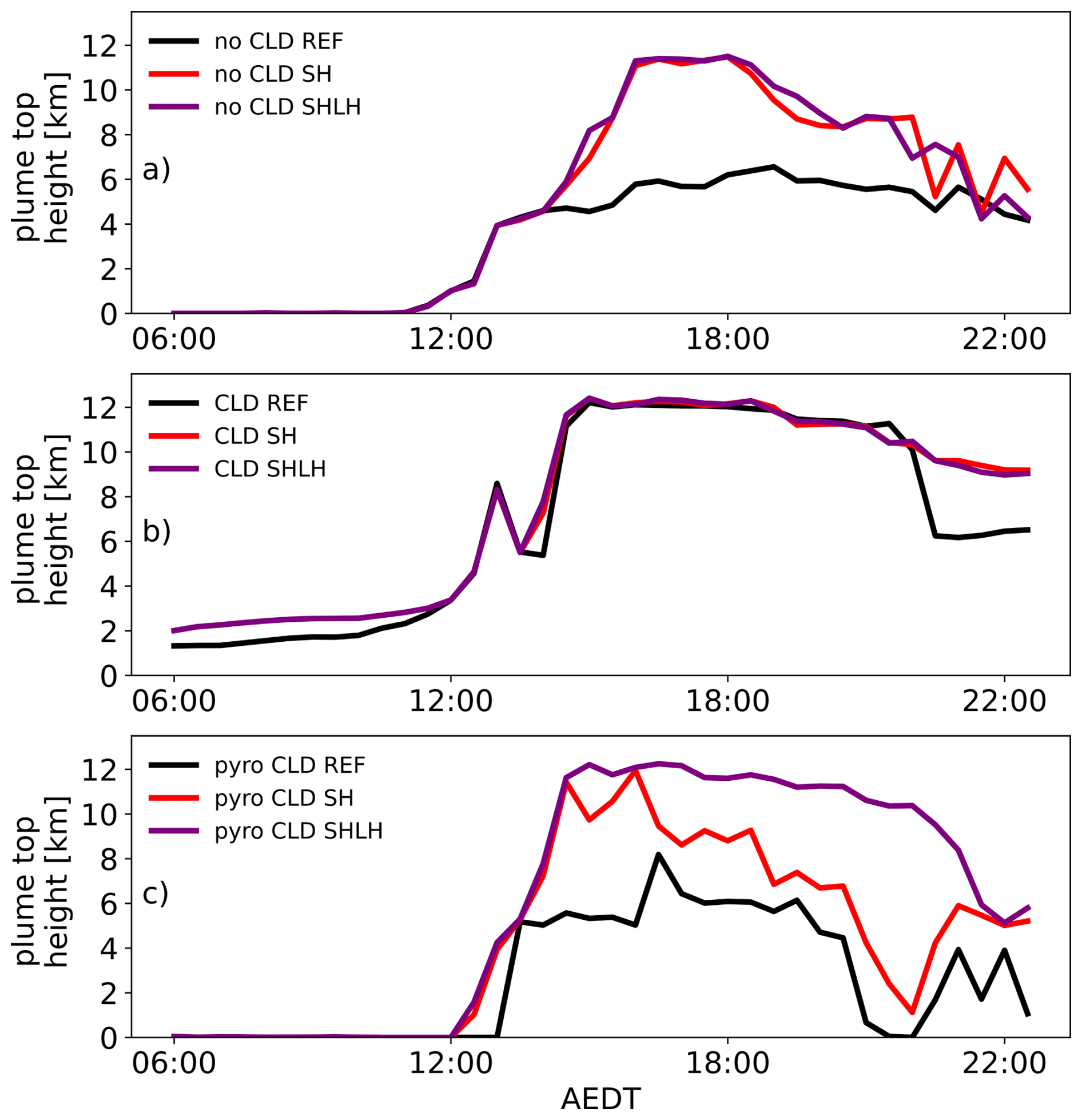
Figure 7 Temporal evolution of plume top height throughout the day (AEDT) for three experiments – REF (black), SH (red), and SHLH (purple) – for (a) the plume area without clouds, (b) the plume area where clouds are also present, (c) the area where a pyro-convective cloud has formed.

Lastly, Fig. 7c shows the evolution of the plume height within the newly forming pyro-convective cloud. Here, the masked grid points only exceed 100 in the afternoon, with masked grid points of the order of 10⁴ for the SHLH and SH experiments and of the order of 10³ for the REF experiment. The plume top height is 0 up to 12:00 AEDT, as no pyro-convective cloud has formed. Then the height increases steeply during the experiments and decreases for REF and SH around 20:00 and for SHLH at 21:00 AEDT onward. The effect of heat and moisture release becomes evident when comparing the top heights during the formation of pyro-convective clouds. Fire-induced heat release increases the top height by up to 6.9 km. Further, the SHLH experiment indicates, through a more uniform profile and later decline, that moisture release increases pyro-convective cloud formation and that more grid cells exceed the threshold and for a longer time. We can see that the enhancement of the plume top height is more visible in cloud-free and pyro-cloud regions. For regions with pre-existing clouds, additional buoyancy is most noticeable in the morning.

4 Discussion

First of all, we discuss the uncertainties that contribute to the differences between the observations and the model. The retrieval itself is subject to uncertainties. The height retrievals depend on the relative viewing geometry of LEO–GEO. The retrieval process estimates the uncertainty of the retrieved parameters using a covariance matrix. This covariance matrix is used to calculate the uncertainty statistics for, beyond other parameters, the retrieved height. The uncertainty derived from the covariance matrix serves as an effective guide to the quality of the retrievals (Carr et al., 2019). The shown retrievals are given with an error range of ±200–300 m, which is consistent with the range reported by Carr et al. (2019).

Additionally, uncertainties persist in the comparison, as it is unclear at which specific mass mixing ratio or optical thickness the plume or cloud is detected by the satellite. Therefore, the comparisons with simulations are strongly dependent on the threshold chosen for the plume and cloud definition. Furthermore, the vertical resolution of the model, which increases with height, introduces a varying uncertainty. The model's vertical resolution in the altitudes between 9 and 15 km ranges from 200 to 250 m. This is comparable to the error range of the observations.

In contrast to the typical diurnal cycle of atmospheric stability and fire intensity, which suggests that pyroCb clouds form in the early to late afternoon, some of the most intense pyroCb activity during the ANY event was observed at night (Peterson et al., 2021). This discrepancy between the diurnal cycle of atmospheric stability and fire intensity and the nighttime pyroCb activity is not captured in the simulation. We showed that the measured FRP strongly deviates from the assumed diurnal cycle function for our case study.

Another significant source of uncertainty comes from the input variables from GFAS, which are based on MODIS FRP measurements. These measurements are affected by interference from clouds and dense smoke plumes. The observations in Fig. 2 show that the pyroCb clouds are close to the fire source. This suggests a possible underestimation of the fire intensity, leading to reduced aerosol, heat, and moisture emissions (Kaiser et al., 2012). Consequently, it becomes challenging to generate sufficient buoyancy to trigger pyro-convective cloud formation.

Further uncertainties are introduced by the analysis methods. The results depend on the selection of thresholds for the plumes and clouds, and therefore the plume heights. The discussed uncertainty due to the vertical resolution becomes critical when calculating the mean of the 100 largest altitudes. This introduces a dependency on the grid cell height, which increases with altitude. This dependency is problematic because it can lead to an overestimation of plume top heights in regions with coarser vertical resolution. As altitude increases, the grid cell heights become larger and the mean value calculation may disproportionately represent higher altitudes, skewing the results. However, we use this approach because it provides a consistent method for identifying the highest plume altitudes across different scenarios. By focusing on the 100 largest altitudes, the method ensures that the most significant plume heights are captured, even if the vertical resolution varies. This consistency is crucial for comparative analysis and for understanding the overall behavior of plume dynamics in different atmospheric conditions.

Furthermore, our simulations do not include aerosol–cloud interactions. While studies such as those of Andreae et al. (2004), Koren et al. (2005), and Wang et al. (2009) report enhanced updrafts due to these interactions, Luderer et al. (2006) found that although aerosol loading significantly alters the microphysical structure of pyro-convective clouds, the influence of cloud condensation nuclei on the dynamic evolution of the pyroCb remains limited. More recent studies by Kablick III et al. (2018) indicated that the impact of fire-generated aerosols in the development of specific pyroCbs were negligible, compared with the effects of fire-generated heat fluxes. Therefore, we assume that the effect of aerosol–cloud interaction is small.

Biomass burning aerosols have the ability to scatter and absorb solar radiation; this can play a significant role in plume rise, as shown by Ohneiser et al. (2023). Moreover, Chang et al. (2021) report aerosol radiative forcing values between −14.8 and −17.7 W m⁻² close to the source; this is of the order of GFAS FRP for smaller fires. However, we focus on intense fires with pyro-convective cloud formation and therefore assume that, in the mixture of aerosol-clouds, neglect of the aerosol radiative effect is valid.

Further, the absence of condensation and gas-phase chemistry is a coarse simplification but, according to the findings of June et al. (2022), condensation and gas-phase chemistry show a minor impact on aerosol size distribution changes, whereas coagulation significantly contributes to particle growth in the early phase of plume development, which we account for.

Our analysis of the impact of additional water vapor agrees with the findings of Trentmann et al. (2006), who state that the emission of water vapor by a fire does not significantly contribute to the energy budget of the convection. However, our results show that moisture release by fires increased the LWP and IWP, thereby enhancing latent heat release, especially in the central and eastern parts of the domain. Therefore, the findings of Luderer et al. (2006), who observed that water vapor plays a less significant role in determining the injection height but enhances the amount of particles reaching upper levels, further agree with our results.

5 Conclusions

This study highlights the critical role of fire intensity and atmospheric stability in pyro-convective cloud formation and discusses remaining uncertainties through a direct comparison with observational data. These results demonstrate that the developed parameterization of heat and moisture release, based on satellite retrievals provided by GFAS, enables the simulation of pyro-convective clouds. However, the developed setup exhibits a temporal delay in the formation of these pyro-convective clouds, compared with observed data. These discrepancies can be attributed to errors in the assumed diurnal cycle of fire activity. Sensitivity studies of the diurnal cycle function could address this issue and help reproduce the observations more accurately. By systematically varying the parameters of the diurnal cycle, we can better understand how different assumptions impact the formation of pyro-convective cells.

Overall, the simulations successfully captured the formation of pyro-convective clouds during the ANY event. The background meteorology, characterized by a highly unstable atmosphere, allows for the formation of convective cloud cells, independently of the heat and moisture generated by the fire. These cells are partially fueled and intensified by the heat and moisture released. Additionally, in the center of the domain, a pyro-convective cloud forms only when accounting for sensible heat and moisture release. This simulation of a real case, involving several fire areas in close proximity, highlights how sensitive cloud formation and plume height are to fire intensity and background meteorology. The different fire areas exhibit different effects on cloud formation and plume height. Sensible heat release has been shown to be the predominant contributor to the formation of pyro-convective clouds. However, the release of moisture enhances cloud formation in the early stages of the formation process, which slightly increases the height of the plumes but increases the amount of aerosols lifted. Further case studies are needed to assess the general applicability of this parameterization in other regions. The developed method can potentially enable the simulation of pyro-convective clouds forming in close proximity to their actual occurrences anywhere on the globe.

Appendix A

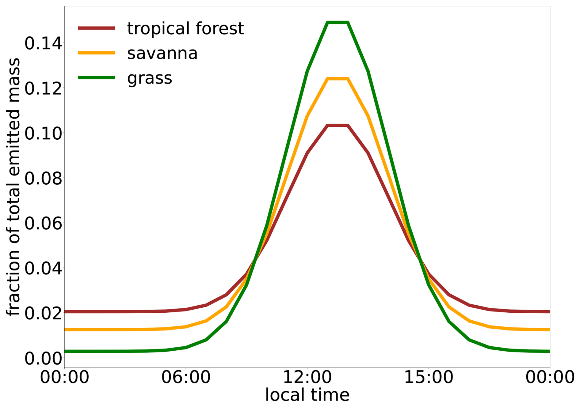
Figure A1 Implemented diurnal cycle function of the emission over the day. The different colors represent the vegetation classes: tropical forest (brown), savanna (orange), and grassland (green). The vegetation class in the experiments is primarily tropical forest.

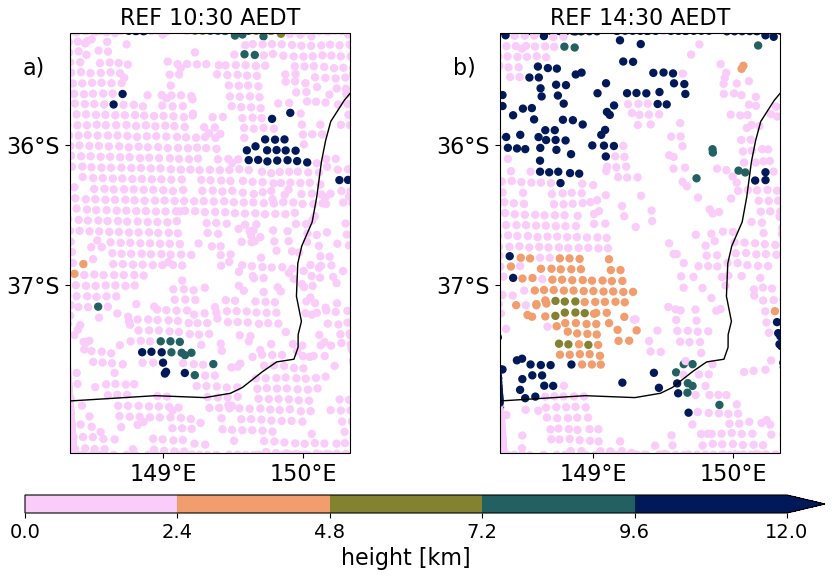
Figure A2 Plume and cloud top heights, simulated for the REF experiment on 30 December 2019 at (a) 10:30 AEDT and (b) 14:30 AEDT.