Long-term satellite trends of European lower-tropospheric ozone from 1996–2017

Tropospheric ozone (O₃) is a harmful secondary atmospheric pollutant and an important greenhouse gas. Multiple satellite records have shown conflicting long-term O₃ trends across regions of the globe, including Europe. Here, we investigate lower-tropospheric sub-column O₃ (LTCO₃, surface – 450 hPa) records from three ultraviolet (UV) sounders produced by the Rutherford Appleton Laboratory (RAL): the Global Ozone Monitoring Experiment (GOME, 1996–2010), the Scanning Imaging Absorption Spectrometer for Atmospheric Chartography (SCIAMACHY, 2003–2011) and the Ozone Monitoring Instrument (OMI, 2005–2017). GOME and SCIAMACHY detect negative trends of approximately −0.2 DU yr⁻¹, while OMI indicates a negligible trend. The TOMCAT 3-D chemical transport model was used to investigate processes driving simulated trends and to identify possible reasons for satellite trend discrepancies. The simulated LTCO₃ trends were negligible (consistent with ozonesonde trends), even when spatiotemporally co-located to the satellite level-2 swath data and convolved by averaging kernels (i.e. a measure of the satellite retrieval vertical sensitivity). Model sensitivity experiments with the emissions or meteorology fixed to 2008 also showed negligible LTCO₃ trends between 1996 and 2018, indicating that changes in emissions and meteorology had a limited impact on LTCO₃ temporal evolution. Given the substantial decrease in air pollutant emissions, this was unexpected, while year-to-year variability dominated the meteorological influence on LTCO₃. Finally, we find a negligible trend in the long-term stratosphere O₃ flux into the free troposphere over this period arriving over Europe. Overall, our observational and modelling analysis indicates that European LTCO₃ trends have been stable between 1996 and 2018.

1 Introduction

Tropospheric ozone (O₃) is both detrimental to air quality and an important short-lived climate forcer (e.g. Monks et al., 2015). At the surface, O₃ is harmful to human health as it is a strong oxidant, with an estimated 24 000 premature deaths attributed to acute O₃ exposure across Europe in 2020 (European Environment Agency, 2022). It is also damaging to plants and reduces crop yields, which is estimated to have caused global economic damage in the region of USD 14–26 billion in 2000 (Van Dingenen et al., 2009). Tropospheric O₃ is a significant greenhouse gas (GHG), with an estimated effective radiative forcing of 0.47 (0.24–0.70) W m⁻² between 1750 and 2019, dominated by changes in tropospheric O₃ (IPCC, 2021; Forster et al., 2021; Skeie et al., 2020). It is a secondary pollutant, produced through reactions involving precursor nitrogen oxides (NO_x, referring to nitrogen dioxide, NO₂, and nitric oxide, NO) and volatile organic compounds (VOCs) in the presence of sunlight. Despite anthropogenic emissions of these precursor gases declining in the last 20 years (European Environment Agency, 2022), in 2021 an estimated 10 % of the European urban population was exposed to O₃ concentrations above the European Union (EU) standards and 94 % above the World Health Organization (WHO) guidelines (European Environment Agency, 2023). These persistent exceedances across Europe highlight the need for further study into how near-surface O₃ is changing over time.

Satellite retrievals of tropospheric trace gases present an opportunity to enhance our knowledge of atmospheric composition on larger spatial scales (e.g. global or regional) than other observations. Trends in satellite tropospheric O₃ retrieved from different instruments have been shown to not be consistent for some regions around the world. Gaudel et al. (2018) presented long-term trends for several satellite tropospheric-column O₃ products, finding a range of trends from −0.50 to +0.16 DU yr⁻¹ for the 30–60° N latitude band, which includes Europe. These inconsistent trends are from instruments using different measurement technique/spectral ranges, e.g. ultraviolet (UV) and infrared (IR), which have different attributes, such as spatial coverage, resolution and vertical sensitivity. They also use different retrieval schemes, which means different state vectors, a priori information, radiative transfer models, tropopause definitions and cloud filters, and data are presented for different vertical ranges and across different time periods between 1996 and 2016. So, there is a need to study these records in more depth, especially those from similar instruments (e.g. UV here), from the same retrieval scheme and over the same time period, to minimise the most obvious sources of difference between the records. Aside from Gaudel et al. (2018), there are few studies of European long-term trends of tropospheric O₃ from satellite retrievals. Ebojie et al. (2016) found a non-significant negative trend of −0.9 ± 0.5 % yr⁻¹ for southern Europe between 2003 and 2011 using tropospheric-column data from the Scanning Imaging Absorption Spectrometer for Atmospheric Chartography (SCIAMACHY). Pope et al. (2018) found no significant trends between 2005 and 2015 across England and Wales for the sub-column O₃ (0–6 km) from the Ozone Monitoring Instrument (OMI) retrieved by the Rutherford Appleton Laboratory (RAL) scheme. However, they found a significant positive O₃ trend in Scotland (representing background O₃) of 0.172 Dobson units (DU) yr⁻¹.

The number of studies of long-term variation in European free tropospheric O₃, e.g. from other measurement techniques such as ozonesondes and aircraft, is fairly limited and provides a mixed story. From ozonesondes launched from a European site, Oltmans et al. (2013) found O₃ in the 500–700 hPa layer to have increased from the beginning of the 1970s to the end of the 1980s and to have then declined slowly to 2010. They found a trend of between ∼ 3 % and 5 % per decade at the surface – 300 hPa for 1970–2010 but near-zero trends when only 1980–2010 is considered. Logan et al. (2012) showed increasing O₃ from regular aircraft measurements (from the Measurement of OZone and water vapour by Airbus In-service airCraft (MOZAIC) programme) during the 1990s and showed that the ozonesondes, surface high-altitude alpine sites and aircraft agree on decreasing O₃ since 1998. Gaudel et al. (2018) found little change in ozonesonde observations above southern France in 1994–2013. The In-service Aircraft for a Global Observing System (IAGOS) commercial aircraft monitoring network highlighted O₃ increases in winter (11 % increase) and autumn (5 % increase) above Frankfurt, Germany (300–1000 hPa), in a comparison of 1994–1999 and 2009–2013, but there was little change in spring and summer (Gaudel et al., 2018). Two recent studies looking across the whole of Europe found quite similar results in trends of median O₃. Gaudel et al. (2020) found a small trend between 1994 and 2016 from aircraft observations of 1.3 ± 0.2 ppbv per decade (2.4 %) for 700–300 hPa; and Christiansen et al. (2022) found trends of between ∼ −1 and 4 ppb per decade across seven European ozonesonde sites from 1990–2017 in the free troposphere, with an average of 1.9 ± 1.1 ppb per decade (3.4 ± 2.0 % per decade). Chang et al. (2022), using a merged IAGOS–ozonesonde dataset, found positive trends in the free troposphere (700–300 hPa) of 0.63 ± 0.24 ppbv per decade, but in the boundary level (950–800 hPa) there were negligible trends over Europe. Wang et al. (2022) found similar results, with weak positive tropospheric-ozone trends (< 1.0 ppbv per decade) over Europe between 1995 and 2017.

Here, we study three RAL UV satellite records (Global Ozone Monitoring Experiment (GOME), SCIAMACHY and OMI) in detail between 1996 and 2017, exploring long-term trends of lower-tropospheric column ozone (LTCO₃ – surface to 450 hPa) across Europe. We make comparisons using a 3-D chemical transport model (TOMCAT) to provide a common framework for comparing the impact of different sampling and vertical sensitivity between the instruments. The averaging kernels (AKs), provided with RAL Space's ozone products from satellite UV–Vis nadir sounders, provide the vertical sensitivities of the different layers retrieved with the optimal estimation approach applied to the respective instruments (as discussed in Miles et al., 2015). Pope et al. (2023b) provide a detailed assessment of the RAL Space AKs (e.g. Figs. 1 and 2 of that study), finding that peak tropospheric O₃ sensitivity is in the lower-tropospheric layer (surface – 450 hPa), which is the focus of this study. To allow direct like-for-like comparisons of models (e.g. TOMCAT) with these satellite datasets, AKs (i.e. for each layer, essentially a vertical weighting of the retrieval sensitivity) need to be mapped onto the modelled vertical profile before comparable quantities (e.g. LTCO₃) can be compared. Here, we use the TOMCAT model as a tool to help investigate the impact of the AKs (i.e. vertical sensitivity) on satellite-derived LTCO₃ trends over Europe (i.e. how substantially the satellite AKs influence the simulated LTCO₃ trends). We also present trends for the ozonesonde record and TOMCAT-simulated tropospheric O₃ across the study period. Lastly, we use model experiments to identify the relative impacts of meteorology and emissions on the model trends across Europe.

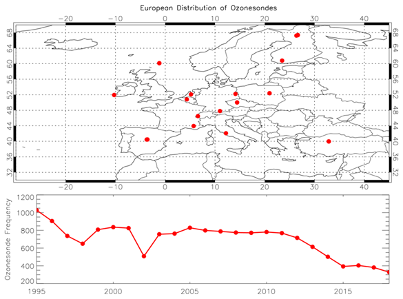
Figure 1 European distribution of ozonesondes used in this study and time series of annual ozonesonde frequencies (i.e. all sites and times).

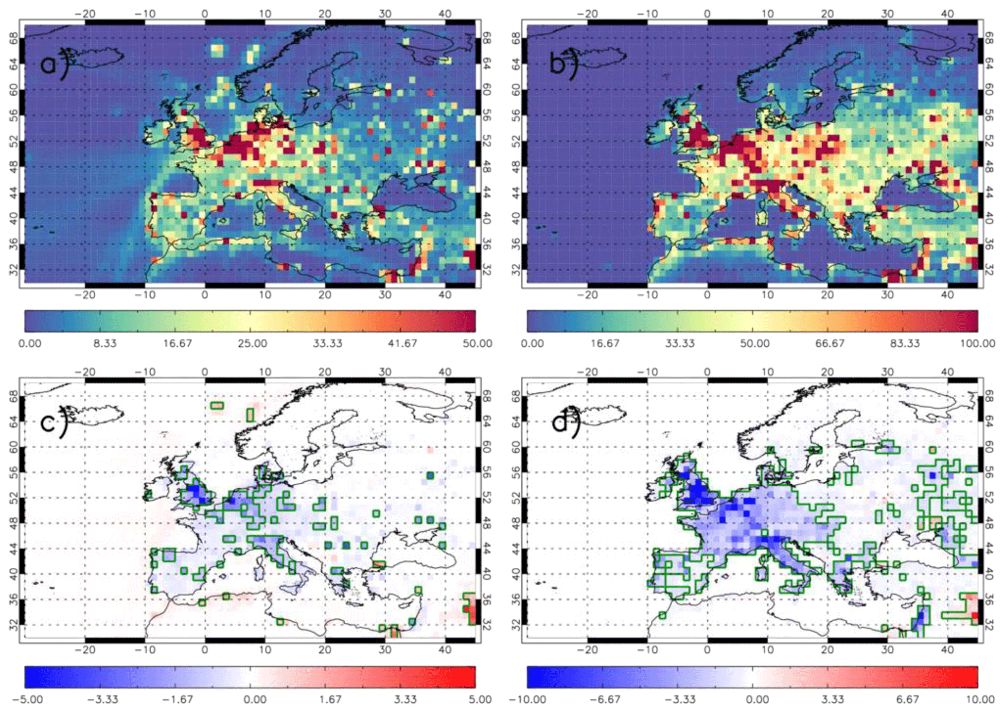
Figure 2 Average TOMCAT emissions (Gg) between 1996 and 2017 for (a) NO_x and (b) carbon monoxide (CO). TOMCAT emission trends (Gg yr⁻¹) between 1996 and 2017 for (c) NO_x and (d) CO. Green polygon-outlined regions show substantial emission trends with p values < 0.05.

2 Methods

2.1 RAL UV satellite data products

We use three records of satellite LTCO₃ from the RAL UV scheme (Miles et al., 2015; Munro et al., 1998). The scheme provided the first satellite retrievals of tropospheric O₃ (Munro et al., 1998), and the subsequent tropospheric O₃ products have been used across a variety of studies including Gaudel et al. (2018). The scheme is based on the standard optimal estimation technique by Rodgers (2000) and is described in detail in Miles et al. (2015), including the treatment of errors. A comparison of the RAL Space UV–Vis satellite products with ozonesondes on a wider scale (i.e. Keppens et al., 2018) found a 10 %–40 % positive bias, comparable to the magnitude of other satellite lower-tropospheric ozone products in the same study. Therefore, all three satellite products have been adjusted for their ensemble mean biases with respect to ozonesondes as a function of the month of the year and the latitude (30° bins; see Russo et al., 2023; Pope et al., 2023b, 2024b). Applying these corrections is intended to mitigate systematic differences between the three instruments' biases while maintaining their temporal variability and evolution. We select from the dataset only sub-columns with an effective cloud fraction of < 0.2, a solar zenith angle of < 80°, the retrieval convergence flag set to 1.0 and the normalised cost function of < 2.0. We define the European domain as 30–70° N and 30° W–45° E.

2.1.1 GOME

The GOME instrument was aboard the European Space Agency (ESA)'s second European Remote Sensing Satellite (ERS-2), which was launched in April 1995 and ceased operation in 2011 (Burrows et al., 1999; European Space Agency, 2022). ERS-2 had a sun-synchronous and near-polar orbit, with an Equator crossing time of 10:30 LST (local solar time). The instrument had 1-D detector arrays providing spectral sampling across four contiguous bands deployed in a nadir across-track scanning mode, a swath width of 960 km, a ground-pixel resolution of 40 km (along-track) × 320 km (across-track) and achieved global coverage in ∼ 3 d. GOME measured in the UV-near-IR (NIR) wavelength range (240–790 nm) at a spectral resolution of 0.2–0.4 nm (Burrows et al., 1999).

2.1.2 SCIAMACHY

The SCIAMACHY instrument was aboard ESA's Envisat, which was launched in March 2002 and ceased operation in April 2012 (Bovensmann et al., 1999; Ebojie et al., 2016). Envisat had a sun-synchronous and near-polar orbit, with an Equator crossing time of 10:00 LST. The instrument had 1-D detector arrays, like GOME, deployed in limb-scanning, nadir-scanning and solar/lunar occultation viewing modes. In nadir-scanning mode, it had an across-track width of 960 km and a ground-pixel resolution of 30 km (along-track) × 240 km (across-track). SCIAMACHY measured in the UV-NIR as for GOME and also two SWIR bands spanning a wavelength range of 240–2380 nm at a spectral resolution of 0.2–1.5 nm (Bovensmann et al., 1999).

2.1.3 OMI

The OMI instrument is aboard NASA's Aura satellite, launched in July 2004 and currently still in operation (Levelt et al., 2006). The Aura satellite has a sun-synchronous and near-polar orbit with an Equator crossing time of 13:45 LST and flies as part of the “A-train” formation. The instrument uses a 2-D detector array in a nadir-scanning mode, with the second dimension providing continuous across-track sampling. It has a swath width of 2600 km and a ground resolution of 13 km × 24 km, providing nearly global coverage every day. OMI measures in the UV–Vis wavelength range (270–500 nm) with a spectral resolution of 0.45–1.0 nm (Levelt et al., 2006). Due to the 2-D detector array of OMI, across-track adjustments were calculated for each detector row and year (relative to an average of all rows) to reduce enhanced stratospheric influence from the longer viewing path at the edges of the swath.

2.1.4 Uncertainties

The satellite instruments used here have several known issues, e.g. the OMI detector row anomaly (Levelt et al., 2018), the GOME tape recorder failure (Van Roozendael et al., 2012) and UV degradation for GOME-type sensors (e.g. Miles et al., 2015). Due to the OMI row anomaly, there is a reduction in the availability of data from some positions across the swath from ∼ 2009 onwards, predominantly from the middle of the swath. To account for this, we have selected rows with a consistent seasonal cycle amplitude and shape for the years for which they are available. We calculate across-track adjustments (relative to an average for all rows) for the available rows on a yearly basis to account for the changing number of rows used. The GOME tape recorder failure mostly impacted the Southern Hemisphere (SH) so had little impact on the European domain used here. To account for UV degradation in GOME and SCIAMACHY, a correction has been applied by RAL prior to the L2 (retrieval) processing step (see Miles et al., 2015), based on the ratio of UV sun-normalised radiance spectra modelled from a climatology and observed sun-normalised radiances.

As noted above, all three satellite L2 datasets have been compared with ozonesonde ensembles and corrections applied as functions of latitude and month of the year to reduce relative systematic errors between the three products (see Russo et al., 2023). As in Pope et al. (2015), when multiple soundings are averaged together to form a monthly mean, these random errors will reduce by a factor of $\frac{\mathrm{1}}{\sqrt{N}}$ (where N is the sample size). We present an estimate of these monthly average random errors across the European domain. Here, the satellite random error is calculated for each grid box using daily gridded data (where there are available data) for the necessary time period (thus N = the number of days with suitable data and the grid box average random error is scaled by $\frac{\mathrm{1}}{\sqrt{N}}$). Typically, we find the domain-average monthly random error to be 31.6 (21.4–47.7) %, 31.1 (23.1–44.9) % and 31.5 (21.9–49.3) % for GOME, SCIAMACHY and OMI, respectively. However, when reducing by $\frac{\mathrm{1}}{\sqrt{N}}$ (i.e. number of days in the month), this reduces to 4.1 (2.4–7.2) %, 4.2 (2.8–9.0) % and 2.6 (1.3–4.8) %, respectively.

2.2 Ozonesondes

We present ozonesonde data from 1996–2018 from the World Ozone and Ultraviolet Radiation Data Centre (WOUDC, 2021), which predominantly uses electrochemical concentration cell (ECC) and Brewer–Mast ozonesondes. The ozonesondes are filtered for records in the European domain and within 3 h of each satellite overpass time (10:00 and 13:30 LST). The ozonesonde profiles are used to derive LTCO₃. Co-located TOMCAT records were produced, using the nearest model grid-box value for each ozonesonde profile. The location of the European ozonesondes (and annual frequency) used in this study is shown in Fig. 1.

2.3 TOMCAT 3-D model

TOMCAT is a global 3-D offline chemical transport model forced by ERA-Interim meteorological reanalyses from the European Centre for Medium-Range Weather Forecasts (ECMWF; Chipperfield, 2006; Dee et al., 2011; Monks et al., 2017). It has a resolution of 2.8° × 2.8° with 31 vertical levels from the surface and 10 hPa. TOMCAT is coupled with the Global Model of Aerosol Processes (GLOMAP), which calculates aerosol microphysics (Mann et al., 2010; Spracklen et al., 2005). The full chemistry scheme, with 79 species and ∼ 200 chemical reactions, is described in Monks et al. (2017). Anthropogenic surface emissions for NO_x, CO and VOCs are from the Coupled Model Intercomparison Project Phase 6 (CMIP6; Feng et al., 2020). Fixed natural surface emissions (soils/ocean) for NO_x, CO and VOCs are from POET (Precursors of Ozone and their Effect on the Troposphere; Granier et al., 2005; Olivier et al., 2003). Fixed annual biogenic emissions of CO and VOCs are from the Chemistry–Climate Model Initiative (CCMI; Morgenstern et al., 2017). Annual varying biogenic emissions of isoprene and monoterpenes are from the Joint UK Land Environment Simulator (JULES) in the free-running UK Earth System Model (UKESM; Sellar et al., 2019) from a CMIP6 historical setup (Clark et al., 2011; Sellar et al., 2019). Biomass burning emissions are from the Global Fire Emissions Database (GFED) version 4 (van der Werf et al., 2017). Aerosol surface emissions (sulfur dioxide, black carbon, organic carbon) are from MACCity (Granier et al., 2011). Global average surface TOMCAT methane (CH₄) is scaled to the annually varying global average surface CH₄ value from the National Oceanic and Atmospheric Administration (NOAA; Dlugokencky, 2020) while retaining its simulated spatial distribution due to emissions and sinks.

Using TOMCAT, we simulated tropospheric O₃ between 1996 and 2018, with 1 year of spin-up. We present satellite records with two different Equator crossing overpass times, approximately 10:00 for Envisat (SCIAMACHY) and ERS-2 (GOME) and approximately 13:30 for Aura (OMI); therefore, the simulations here have been set up to sample 3-D fields of the model daily at these two LSTs. This control configuration of TOMCAT is labelled TC-CTL. To identify the relative impact of surface emissions and meteorology on long-term trends, we performed two model experiments. Figure 2 shows the surface emissions for NO_x and carbon monoxide (CO), key O₃ precursor gases and their tendencies between 1996 and 2017. The NO_x (Fig. 2a) and CO (Fig. 2b) emission long-term averages peak over northwestern Europe at > 10 and > 100 Gg per grid box. The corresponding trends (Fig. 2c and d) show substantial (p value < 0.05 – green polygon-outlined regions) decreases of < −5.0 and < −10 Gg yr⁻¹. Therefore, one experiment used a fixed year of monthly surface emissions (from 2008, around the midpoint of the study period) and varying meteorology (TC-FX-EMS). The other used a fixed year of meteorology reanalyses to force the model (from 2008) and varying surface emissions (TC-FX-MET). While there are many non-linear processes controlling the spatiotemporal evolution of tropospheric O₃ (e.g. temperature, advection, deposition, photochemistry, stratosphere–troposphere exchanges, different precursor emission sources such as anthropogenic sources and wild fires), it is not practical in this study to undertake a 22-year sensitivity experiment for each process. Pope et al. (2023a) did undertake a detailed assessment of factors contributing to the 2018 European summer tropospheric O₃ event, focussing on 2017 and 2018. Therefore, we limited ourselves to the fixed emissions and meteorology experiments between 1996 and 2017. Here, the fixed meteorology experiment refers to influences of meteorological variables like temperature, cloud cover (i.e. influence on photochemistry) and then long-range transport (e.g. advection of O₃-rich air masses). For all TOMCAT simulations, we calculate and present LTCO₃. For cases where there is comparison with the satellite records, the TOMCAT simulations are co-located with the satellite records and have averaging kernels (AKs) applied. Where we are inter-comparing model simulations (or with the ozonesondes, which have no issues with vertical sensitivity as they are in situ measurements with high vertical resolution), application of the satellite AKs to the model is not required.

A tracer (O_3S) for stratosphere–troposphere exchange (STE) is used from the TOMCAT simulations to understand the impact of O₃ transport from the stratosphere. The tracer is set equal to the model-calculated O₃ in the stratosphere. When the tracer enters the troposphere, there are no additional sources of the tracer, as the only tropospheric source of the tracer is transported from the stratosphere. In the troposphere, all sink reactions for O₃ apply, e.g. photolysis and reaction with OH and HO₂, as well as dry deposition (Monks et al., 2017). Any O₃ that is transported into the stratosphere will be labelled as stratospheric before it returns. Note that the model does not contain any specific treatment of stratospheric chemistry (e.g. chlorine, bromine, polar stratospheric clouds) as it uses a climatological ozone vertical boundary condition. However, the flux of air between the lower stratosphere and upper troposphere is well represented in the model (i.e. driven by meteorological reanalyses).

2.4 Trend model

We use the following trend model with a seasonal component, as shown in Eq. (1):

$$\begin{array}{}\text{(1)}& Y_t=C+B{X}_t+A\sin (\mathit{\omega }{X}_t+\mathit{\varphi })+N_t,\end{array}$$

where Y_t is the monthly sub-column O₃ for month t, C is the sub-column O₃ for the first month of the record, X_t is the number of months after the first month of the record, Asin (ωX_t+ϕ) is the seasonal component (A is the amplitude, ω is the frequency (with the period set to 1 year, $\mathit{\omega }=\frac{\mathit{\pi }}{\mathrm{6}}$) and ϕ is the phase shift). N_t represents the model errors/residuals that are unexplained by the fit function, including interannual variability. C, B, A and ϕ represent the fit parameters which are based on a linear least-squares fit. This trend model is based on a function in Weatherhead et al. (1998) and has been used in several studies looking at long-term trends in tropospheric species (e.g. van der A et al., 2006; van der A. et al., 2008; Pope et al., 2018, 2024b). Weatherhead et al. (1998) give a derivation for the precision of the trend as a function of the autocorrelation, the length of the time series (in months) and the variance in the fit residuals. The trend precision, σ_B, is calculated by Eq. (2):

$$\begin{array}{}\text{(2)}& {\mathit{\sigma }}_B\approx \left[{\displaystyle \frac{{\mathit{\sigma }}_N}{n^{\frac{\mathrm{3}}{\mathrm{2}}}}}\sqrt{{\displaystyle \frac{(\mathrm{1}+\mathit{\alpha })}{(\mathrm{1}-\mathit{\alpha })}}}\right],\end{array}$$

where n is the number of years in the record, α is the autocorrelation in the residuals and σ_N is the standard deviation in the residuals. In this study, trends are presented in DU yr⁻¹ (and % yr⁻¹) with ± the precision (σ_B) × 2 (i.e.  ±  represents the 95 % confidence intervals).

3 Results

3.1 Long-term satellite records

LTCO₃ from three satellite records (GOME, SCIAMACHY and OMI) between 1996 and 2018 is shown in Fig. 3. The three records show an LTCO₃ seasonal cycle with higher values (around 25.0–30.0 DU) in summer and lower values (around 15.0–20.0 DU) in winter, with an average seasonal “amplitude” of 9.6, 10.8 and 11.7 DU for GOME, SCIAMACHY and OMI, respectively. SCIAMACHY and GOME show a large variation between years in seasonal cycle “amplitude” (the difference between the maximum and minimum month for each year), with a standard deviation of ∼ 2.2 and 1.8 DU, respectively, whereas OMI shows a smaller variation, with a standard deviation of ∼ 1.1 DU. Broadly, the GOME LTCO₃ time series indicates an underlying decrease from 1996–2002/2003 and then a stabilisation to 2010. For SCIAMACHY, the LTCO₃ record is relatively consistent but shows two large peaks (> 25.0 DU) in the summers of 2007 and 2008. In contrast, the OMI LTCO₃ record shows a distinctive pattern over the record, decreasing towards 2009, increasing towards ∼ 2015 and afterwards beginning to decrease again. The three satellite records have 6 overlapping years (2005–2010); this allows for a direct intercomparison (Fig. 3b). Across these overlapping years, GOME and SCIAMACHY show similar LTCO₃ absolute values, aside from the higher summer values in 2007 and 2008 for SCIAMACHY, with an average difference of 0.5 DU (Fig. 3). The OMI values are on average 4.5 DU larger than GOME and 3.9 DU larger than SCIAMACHY. This is despite having applied adjustments to each record based on the mean differences with respective ozonesonde ensembles (see Russo et al., 2023, and Pope et al., 2024a, for details). Although there is a moderate absolute offset between them, OMI and SCIAMACHY show a high correlation (Pearson's correlation coefficient (r) = 0.91), with lower correlations between GOME and SCIAMACHY (r = 0.62) and GOME and OMI (r = 0.64) due to GOME's LTCO₃ seasonal cycle lagging the other two instruments by approximately 1 month. During the overlap years, GOME has the seasonal cycle with lowest amplitude: 8.5 DU in comparison to 11 DU for SCIAMACHY and OMI. It is notable that UV degradation of the GOME instrument in this latter period of its operational lifetime had been substantial, giving rise to low optical throughput, correspondingly low signal-to-noise and a large correction becoming necessary to sun-normalised UV radiances. The differences found here between the instruments could also be due to several other factors, such as overpass time (e.g. diurnal variation in boundary layer thickness and/or O₃ mixing ratios), spatial sampling and vertical sensitivity (itself a function of signal-to-noise).

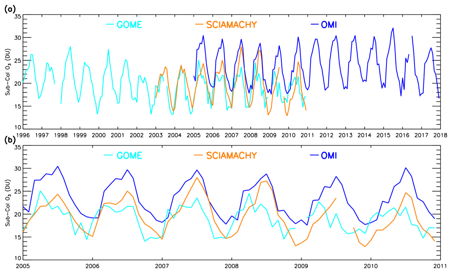
Figure 3 Time series of European monthly average satellite lower-tropospheric column O₃ (LTCO₃, surface – 450 hPa) (DU) for (a) 1996–2017 full record and (b) 2005–2010 overlap period. The Pearson's correlation coefficient (r), 2005–2010, between the GOME-SCIAMACHY, GOME-OMI and SCIAMACHY-OMI time series are 0.62, 0.64 and 0.91, respectively. The average differences are −0.5, −4.5 and −3.9 DU, respectively.

Here, the model acts as a useful framework to investigate the impact of satellite vertical sensitivity on retrieved LTCO₃ quantities (e.g. absolute values, trends) but also a further constraint on European LTCO₃ spatiotemporal evolution. Thus, the TOMCAT-simulated tropospheric O₃ record has been co-located with each satellite retrieval and convolved by the AKs shown in Eq. (3):

$$\begin{array}{}\text{(3)}& \mathit{m}\mathit{o}{\mathit{d}}_{\text{AK}}=\mathbf{AK}(\mathit{m}\mathit{o}{\mathit{d}}_{\text{int}}-\mathit{a}\mathit{p}{\mathit{r}}_{\text{hi}})+\mathit{a}\mathit{p}{\mathit{r}}_{\text{low}},\end{array}$$

where mod_AK is the vector of modified model sub-columns (Dobson units, DU), AK is the averaging kernel matrix and mod_int is the vector of model sub-columns (DU) on the satellite retrieval pressure grid. Here, the AK is rectangular (23 × 19 levels), so the a priori has two forms: (1) apr_hi representing 23 sub-columns and (2) apr_low representing 19 sub-column levels.

Direct comparisons of GOME and SCIAMACHY with TOMCAT show a model overestimation of approximately 4.0 DU and correlation coefficients of 0.72 and 0.82, respectively (Fig. 4). In contrast, for OMI, the model underestimates, with a mean difference of −1.1 DU. Applying the AKs to the model record improves the agreement with GOME and SCIAMACHY, broadly decreasing the model LTCO₃ record by approximately 2.6 DU in both cases and improving the correlation coefficients from 0.72 to 0.74 for GOME and from 0.83 to 0.92 for SCIAMACHY. For OMI, the application of the AKs also decreases the sub-column values; however, this increases the underestimate by the model from 1.1 to 4.0 DU, and it causes a reduction in the correlation from 0.83 to 0.78.

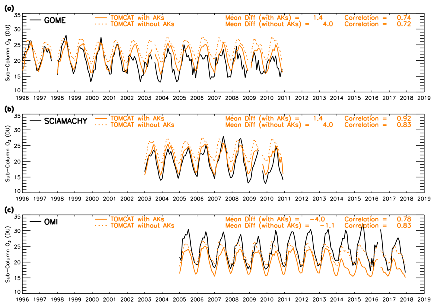
Figure 4 Time series of European monthly average LTCO₃ (DU) between 1996 and 2017 for (a) GOME, (b) SCIAMACHY and (c) OMI. Co-located model records (with and without AKs applied) for each satellite record are also shown. The correlations and mean differences between the model and respective satellite records (TOMCAT satellite, DU) are shown at the top of each panel.

3.2 Satellite, model and ozonesonde LTCO₃ trends

We present European domain-wide trends for the three satellite instruments, the ozonesonde records and the co-located model records (with and without AKs applied for the satellite comparisons) (Table 1). Across the 15-year GOME record, there is a negative trend of −0.21 ± 0.05 DU yr⁻¹ (−1.05 ± 0.26 % yr⁻¹). This negative trend is not captured in the model record, with TOMCAT both with/without GOME AKs applied, showing a near-zero trend. There is a small negative trend of −0.20 ± 0.14 DU yr⁻¹ (−1.03 ± 0.26 % yr⁻¹) across the 8-year SCIAMACHY record. This trend is also not captured in the model record, as TOMCAT (both with/without SCIAMACHY AKs applied) shows near-zero trends. For GOME and SCIAMACHY, although TOMCAT with or without the AKs captures the satellite trends, applying the AKs does subtly change the simulated trend towards that of the satellite, i.e. it makes the model trend more negative. For OMI, there is a near-zero trend across its 13-year record, although there is large interannual variability within this period. Interestingly, this near-zero trend is not captured by the model, as TOMCAT with OMI AKs applied shows a negative trend of −0.26 ± 0.07 DU yr⁻¹ (−1.30 ± 0.37 % yr⁻¹), due to low values around 2014–2018. In contrast, the TOMCAT record without AKs applied shows a near-zero trend across this period, as does the OMI LTCO₃ record itself. Other studies of free tropospheric O₃ trends from observations have found that these trends are not captured by a model (e.g. Parrish et al., 2014; Young et al., 2018; Christiansen et al., 2022). Model trend underestimates (i.e. in terms of magnitude) may be due to uncertainties in prescribed precursor gas emissions and model representation of STE. Christiansen et al. (2022) and Pope et al. (2023a) found dynamics (e.g. STE) to be the more important process controlling the spatiotemporal evolution of free tropospheric ozone in models, while precursor emissions are more important at the surface. Overall, the satellite records here suggest a small reduction in lower-tropospheric O₃ in the early part of the record, which has then stabilised towards the end of the record.

Table 1 Satellite, ozonesonde and model LTCO₃ trends (DU yr⁻¹ and % yr⁻¹) for their respective time periods. For each satellite instrument (GOME, SCIAMACHY and OMI), the co-located model records with and without AKs applied are also presented. The ozonesonde trends are presented for two local time intervals (T₁ = 10.00 LT and T₂ = 13.30 LT) and with co-located model records. CI = confidence interval. Here, TC = TOMCAT and CTL = TOMCAT control simulation. The trend p values are also shown.

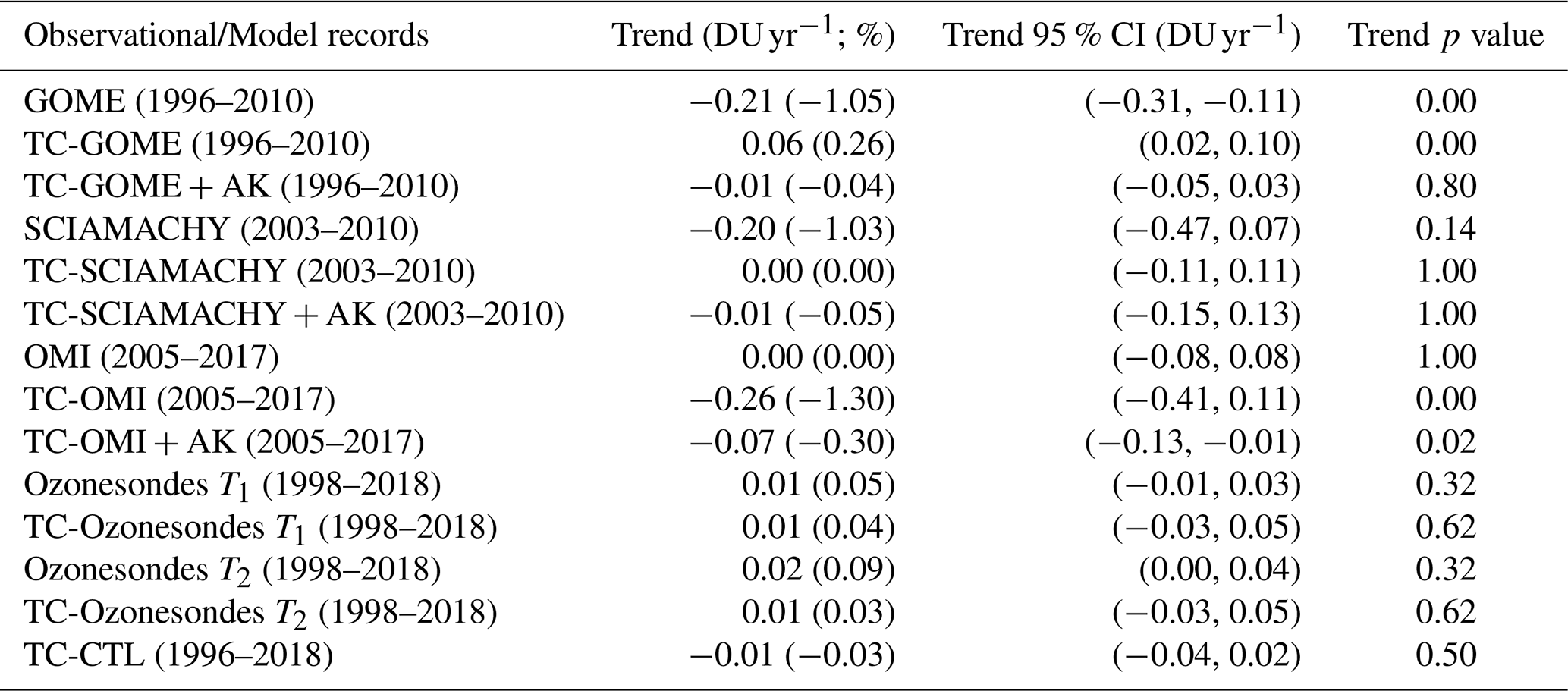
The European ozonesonde record (for 10:00 ± 3 h and 13:30 ± 3 h) between 1996 and 2018 show a near-zero trend for both local time intervals, of 0.01 ± 0.01 and 0.02 ± 0.01 DU yr⁻¹, respectively (Table 1). This near-zero trend is captured in the co-located TOMCAT records, with trends of 0.01 ± 0.01 DU yr⁻¹ for both time ranges, and they show generally good agreement (r = 0.90 for both time ranges). These near-zero trends are smaller than ozonesonde trends presented in Christiansen et al. (2022) for Europe (∼ +3 % per decade). However, in addition to a different selection of sondes used, their ozonesonde record starts in the early 1990s, a time period in which several studies found positive trends in the free troposphere, e.g. Logan et al. (2012), before the stabilisation after ∼ 2000. TOMCAT (not co-located) shows a similar trend to the ozonesondes, with a near-zero trend between 1996 and 2018. This near-zero trend is present despite surface emissions of precursor gases used in the model decreasing during this time period (Fig. 2).

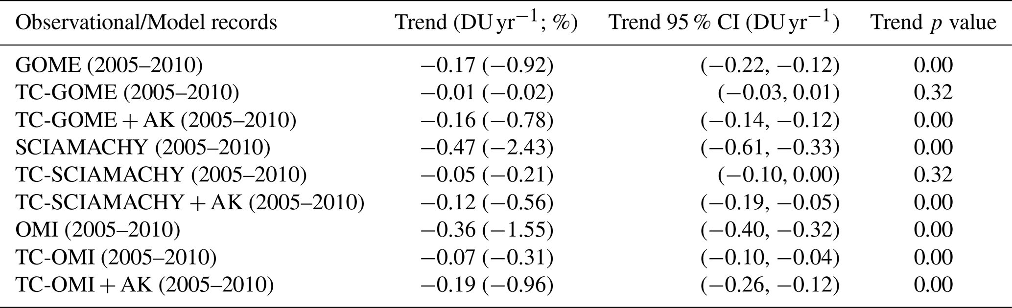
During their overlap period (2005–2010), LTCO₃ trends for all three satellite instruments are negative (Table 2), with GOME showing the lowest (−0.17 DU yr⁻¹, −0.92 % yr⁻¹), SCIAMACHY showing the largest (−0.47 DU yr⁻¹, −2.43 % yr⁻¹) and OMI showing a value in between (−0.36 DU yr⁻¹, −1.55 % yr⁻¹). The corresponding ozonesonde trends at the two overpass times (not shown) between 2005 and 2010 are negligible. The model captures the negative satellite trends across the overlap period more convincingly than across their respective complete time periods (Table 2). The model record co-located to GOME shows a very similar negative trend of −0.16 DU yr⁻¹ (−0.78 % yr⁻¹). For SCIAMACHY and OMI, the co-located model records show smaller negative trends than the satellite, with −0.12 DU yr⁻¹ (−0.56 % yr⁻¹) and −0.19 DU yr⁻¹ (−0.96 % yr⁻¹), respectively. These negative trends are ∼ 25 % and ∼ 50 % the size of the SCIAMACHY and OMI trends, respectively.

Table 2 Satellite, ozonesonde and model LTCO₃ trends for 2005–2010. For each satellite instrument (GOME, SCIAMACHY and OMI), the co-located model records with the AKs applied are also presented. The ozonesonde trends are presented for two local time intervals (T₁ = 10.00 LT and T₂ = 13.30 LT) and with co-located model records. CI = confidence interval. The trend p values are also shown.

3.3 Satellite LTCO₃ spatial trends

As seen in Tables 1 and 2, the satellite LTCO₃ trends tend to be more consistent over the 2005–2010 period. GOME (1996–2010) has a consistent negative trend of approximately −0.15 DU yr⁻¹ across the European domain (Fig. 5). For SCIAMACHY (2003–2010), the trend is more strongly negative at −0.5 to −0.3 DU yr⁻¹ apart from a positive trend (0.2–0.3 DU yr⁻¹) in the south of the domain over northern Africa. OMI (2005–2018) shows near-zero trends across large portions of the domain (0.1 DU yr⁻¹, 60–70° N and −0.1 DU yr⁻¹, 50–60° N) and moderately positive trends (0.2–0.4 DU yr⁻¹) over the Mediterranean and northern Africa (predominantly from changes in precursor emissions; see Fig. 7). For the 2005–2010 period, the LTCO₃ trend is consistently negative for SCIAMACHY (< −1.0 to −0.3 DU yr⁻¹) and OMI (−0.5 to −0.2 DU yr⁻¹) apart from some small positive trends over northern Africa. Therefore, the regional trends in Tables 1 and 2 are broadly representative of most parts of the domain. For GOME, there is again a region of positive trend over northern Africa. Elsewhere the trend is typically −0.4 to −0.2 DU yr⁻¹, although there is more noise in the spatial distribution with a scatter of positive trends (0.1–0.3 DU yr⁻¹). Thus, the negative trend for the domain as a whole is smaller (−0.17 DU yr⁻¹) than for the other two instruments (−0.47 and −0.36 DU yr⁻¹).

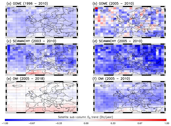
Figure 5 LTCO₃ trends (DU yr⁻¹) for each grid box of the European sub-column satellite records for (a) GOME (1996–2010), (b) GOME (2005–2010), (c) SCIAMACHY (2003–2010), (d) SCIAMACHY (2005–2010), (e) OMI (2005–2018) and (f) OMI (2005–2010).

3.4 Model experiments

We present two additional TOMCAT simulations, one with a repeating fixed year of emissions (TC-FX-EMS) and the other with a repeating fixed year of meteorology (TC-FX-MET), both using the fixed year of either monthly surface emissions or 6 h meteorological fields from 2008. We selected 2008 as it represented an approximate midpoint in the study time period. Both simulations closely represent the control (r = 0.98/0.99 for TC-FX-MET/TC-FX-EMS), with TC-FX-EMS on average 0.41 DU larger and TC-FX-MET 0.16 DU smaller (Fig. 6a). As TC-FX-EMS is larger than the control, this suggests that 2008 was a year of surface emissions that caused higher O₃ concentrations than usual, whereas the meteorology of 2008 (used in TC-FX-MET) is more like an average of the whole time period, as shown by the smaller difference with the control. The monthly anomalies for TC-FX-EMS are very similar to the control (Fig. 6b, r = 0.88), highlighting the importance (less importance) of varying meteorology (emissions) in explaining short-term monthly tropospheric O₃ variation. The TC-FX-MET simulation is less well correlated with the control (r = 0.57), thus again showing the importance of meteorological variability in controlling tropospheric ozone. However, periods do exist where the emissions dominate in importance such as 1998 (potentially linked to the strong El Nino that year) where the TC-FX-EMS run struggles to capture the control simulation anomaly, while the TC-FX-MET more reasonably does so.

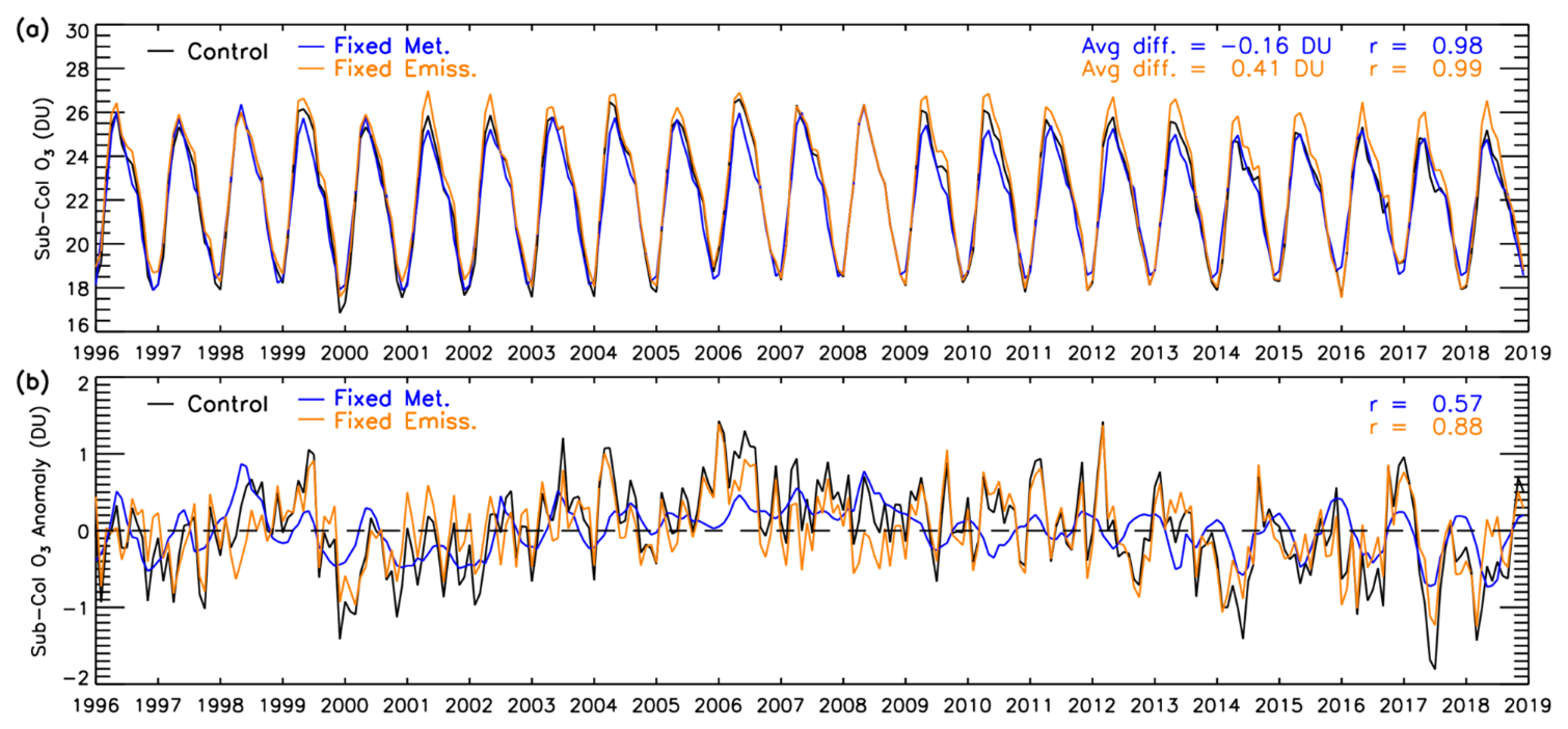
Figure 6 (a) Time series of European average monthly LTCO₃ trends for TOMCAT (control), TC-FX-EMS and TC-FX-MET between 1996 and 2018. The average difference and r of the two experiments and the control is presented in the top right of the panel. (b) Monthly mean anomalies (relative to a 1996–2018 baseline) for the three simulations (DU).

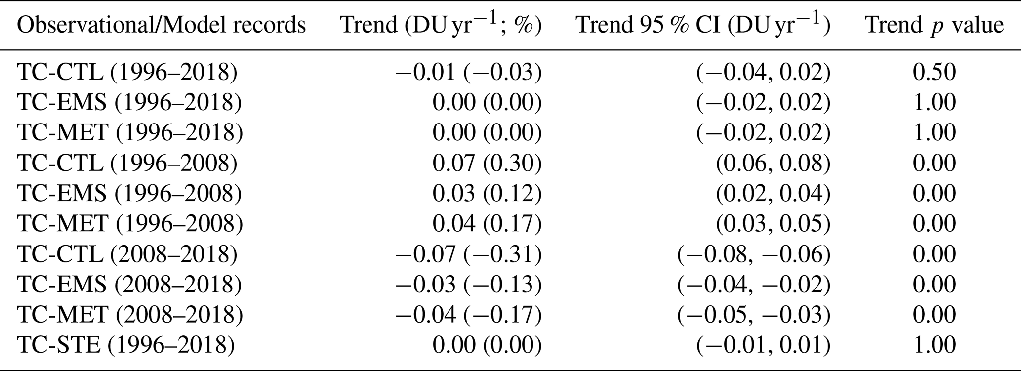
The two fixed simulations show similar near-zero trends to the control between 1996 and 2018 (Table 3). The anomalies of all three simulations show a broadly similar pattern over the time period (Fig. 6b), moving from negative to more positive anomalies between 1996 and ∼ 2006–2008, and then a move from positive to more negative anomalies for the remainder of the time period (∼ 2006–2008 to 2018). For this first time period (1996–2008), the simulations show very small positive trends, with +0.07 DU yr⁻¹ (+0.30 % yr⁻¹) for the control and approximately half the magnitude for both fixed simulations (Table 3). There is a similar story for the second time period (2008–2018) but with very small negative trends, with −0.07 DU yr⁻¹ (−0.31 % yr⁻¹) in the control and, again, approximately half the magnitude for both fixed simulations. This suggests that across both time periods, emissions and meteorology have a similar influence on the long-term trends, rather than a large cancellation of processes. Therefore, the near-zero trend in the control is not due to a cancellation of trends from a large impact of either emissions or meteorology, despite the reduction in key O₃ precursors, e.g. NO_x and VOCs, used in the model.

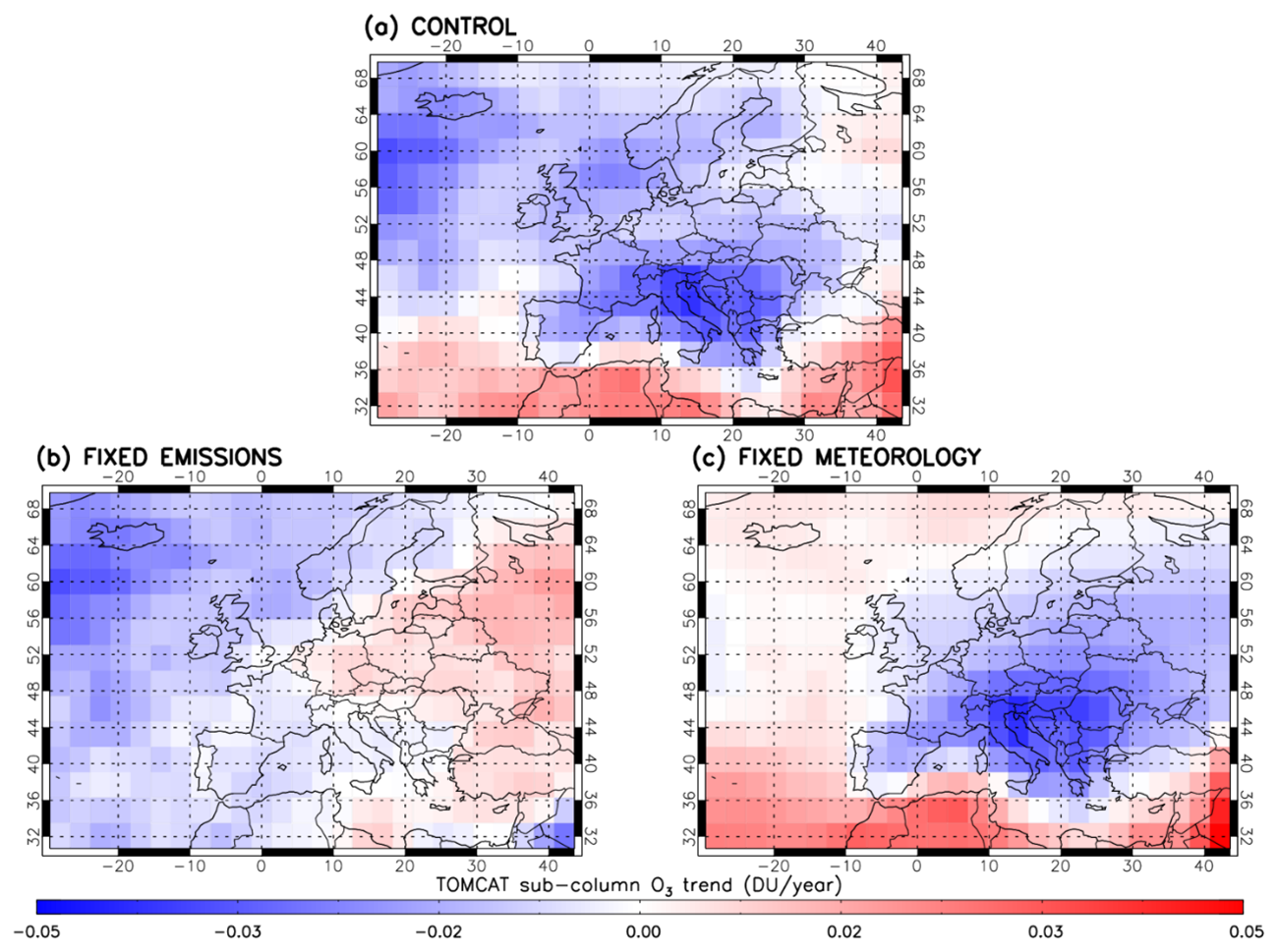
Figure 7 LTCO₃ trends across the European domain (DU yr⁻¹) for (a) TC-control, (b) TC-FX-EMS and (c) TC-FX-MET.

Table 3 Model LTCO₃ trends (DU yr⁻¹ and % yr⁻¹) for 1996–2018, 1996–2008 and 2008–2018 from the TC-CTL, TC-EMS and TC-MET simulations. CI = confidence interval. TC-STE is the TOMCAT tracer for the stratospheric ozone flux into the troposphere, calculated as LTCO₃. The trend p values are also shown.

Spatially, the three simulations show very small trends for each grid box, ranging from −0.04 to 0.05 DU yr⁻¹ (Fig. 7). TOMCAT (control) shows negative trends across central continental Europe, with the largest negative values around Italy and the Balkans and also across the northern Atlantic region. Positive trends are found across the southern Atlantic region, the southern Mediterranean countries in northern Africa and northeastern Europe. The region of negative trends in the control run over central continental Europe. Positive trends in the southern Atlantic region and southern Mediterranean/northern Africa are present in the TC-FX-MET (varying emissions) only and are therefore regions where the long-term trend is dominated by changes in surface emissions from the land. The negative trends in the northern Atlantic region, the North Sea and western Scandinavia and positive trends across northeastern Europe are present in TC-FX-EMS (varying meteorology) only and are regions where the trend is dominated by changes in meteorology. Overall, there is likely some cancellation of regional tendencies in the domain-average LTCO₃ trends for each model experiment (Fig. 7). However, given the absolute magnitude of these pixel-by-pixel-based trends, which are comparable to the overall regional trends (Table 3), it will have a limited impact on the big picture as LTCO₃ appears to be relatively stable in most (if not all) spatial regions.

STE can also impact tropospheric O₃ variation and therefore could influence long-term trends. The simulations use a fixed climatological value of stratospheric O₃ at 10 hPa, but the flux of STE and transport of O₃ into the troposphere varies between the years. Monthly anomalies of a sub-column derived from STE O₃ contribution varied between −0.9 and +0.7 DU (or ∼ −42 % and +21 %) between 1996 and 2018 (Fig. 8). O₃ from STE broadly follows a similar monthly anomaly pattern to the tropospheric sub-column O₃. There is a near-zero trend in the O₃ from STE across the time period (0.00 ± 0.01 DU yr⁻¹), indicating that although STE has impacted year-to-year O₃ variability, there is no strong trend in the simulated STE flux that has influenced tropospheric O₃ in the TOMCAT simulations.

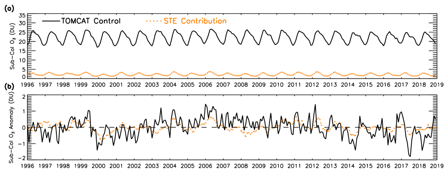
Figure 8 (a) Time series of European monthly average LTCO₃ and STE LTCO₃ (DU) time series from 1996–2018 (DU). (b) Absolute anomalies for both records (DU) (relative to a baseline of 1996–2018).

4 Conclusions

We present a detailed analysis of three satellite products between 1996 and 2017, demonstrating the information they can provide on long-term trends in lower-tropospheric O₃ above Europe. We compare these records with simulated tropospheric O₃ from the 3-D chemical transport model TOMCAT and independent measurements of the free troposphere using ozonesondes.

For the GOME (1996–2010), SCIAMACHY (2003–2010) and OMI (2005–2017) lower-tropospheric O₃ records, there are negative trends of −0.21 ± 0.05 DU yr⁻¹ (−1.05 ± 0.26 % yr⁻¹), −0.20 ± 0.14 DU yr⁻¹ (−1.03 ± 0.26 % yr⁻¹) and a near-zero trend of 0.00 ± 0.04 DU yr⁻¹ (0.00 ± 0.16 % yr⁻¹), respectively. Overall, there appears to have been a decrease in lower-tropospheric O₃ over Europe from the mid-1990s to the early 2000s before a stabilisation in the late 2000s and 2010s, with an increase over the Mediterranean and northern Africa in that latter period (consistent with recent studies, e.g. Pope et al., 2023b, 2024b). Despite reasonable agreement with the satellite records, co-located TOMCAT model records do not capture these small trends, showing predominantly a near-zero trend across the time periods. In contrast to the satellites, observations from the troposphere from ozonesondes agree with the TOMCAT record in showing a near-zero across the time period (1996–2018).

The three satellite records are compared during their 6-year overlap period (2005–2010), showing consistent negative trends (−0.17 to −0.47 DU yr⁻¹), despite there being a systematic offset in the OMI record (∼ 4 DU larger). During this period, the co-located model records show greater consistency with those of the satellites, indicating that considering the vertical sensitivity and spatial sampling does not fully account for the differences seen between the records. The model and ozonesonde trends at the GOME/SCIAMACHY and OMI mid-morning and early afternoon overpasses also suggest that the different diurnal overpasses between the sensors is not a major contributor to differences in detected LTCO₃ trends. Similar results were reported by Pope et al. (2024b), but they did not explore the longer-term records of these multiple sensors between 1996 and 2018 (or use the RAL GOME and SCIAMACHY records). Therefore, additional factors are likely contributing to the instrument differences such as the OMI row anomaly and UV degradation in GOME and SCIAMACHY not being accounted for sufficiently well.

Overall, we have used satellite, ozonesonde and model data to investigate long-term trends in European lower-tropospheric ozone. While there is some agreement between the satellite instruments (i.e. modest negative trends), especially in the overlapping years, the model (with and without the satellite averaging kernels, AKs, applied) and ozonesonde records suggest negligible tendencies. Model sensitivity experiments also suggest that spatiotemporal variability in processes (i.e. precursor emissions, meteorology, and the stratosphere–tropospheric flux) controlling lower-tropospheric ozone have remained stable. As a result, it is difficult to detect a robust and consistent linear trend in European lower-tropospheric O₃ between 1996 and 2017, which is masked by large inter-annual variability in the model and observational records, especially the UV–Vis sensor records. Future trend analyses will benefit for example from new data versions. For example, RAL's scheme has been improved in preparation for full mission re-processing of these and other satellite UV sounders and application to the Sentinel-5 precursor and the upcoming Sentinel-4 and Sentinel-5 missions, which are planned to extend the record to the mid-2040s. Future modelling work – including a more complete description of lower stratospheric ozone, an analysis of chemical budgets and additional model sensitivity experiments (fixing regional emissions for e.g. the Po Valley, which has the largest impact in the TC-FX-MET experiment, although relatively modest in absolute LTCO₃ trend terms) – would be beneficial.