Global optimal estimation retrievals of atmospheric carbonyl sulfide over water from IASI measurement spectra for 2018

Carbonyl sulfide (OCS) is consumed by vegetation during photosynthesis in a one-way hydrolysis reaction, making measuring OCS vegetative uptake a means of inferring and quantifying global gross primary production. Recent studies highlight that uncertainties in OCS surface fluxes remain high and OCS datasets with better spatial coverage are required, particularly from satellite. Here OCS profiles are retrieved using measured radiances from the Infrared Atmospheric Sounding Interferometer (IASI) instruments. We estimate total column amounts over oceanic and inland water regions for the example year 2018, using an optimal estimation scheme, using the University of Leicester IASI retrieval scheme (ULIRS) for selected microwindows in the 2000–2100 cm⁻¹ wavenumber range. Information content exceeds one between ±50° latitude and a peak in vertical sensitivity around 6–10 km (500–300 hPa) in the troposphere. Diurnal variations are limited to ±2 %, showing larger total column amounts at the daytime overpass. The IASI OCS observations show a correlation of at least 0.74 at half the ground-based flask measurement sites compared. Results also agree with the University of Leeds TOMCAT 3-D chemical transport model simulations within ±5 % throughout most tropical regions. This study demonstrates the ability of the IASI instrument to detect OCS in the troposphere and observe a reasonable seasonal cycle indicative of being driven by photosynthesis. Further data acquisition is recommended to gain insight into inter-annual variability in OCS. This novel work will also help improve our understanding of the role of vegetation in the carbon cycle, particularly when utilised in inversion methods.

1 Introduction

Carbonyl sulfide (OCS, also known as COS) is a useful trace gas to help improve our understanding of the terrestrial vegetative uptake of carbon dioxide (CO₂) and the carbon cycle as a whole (Montzka et al., 2007; Berry et al., 2013; Whelan et al., 2018). The net CO₂ budget undergoes annual assessment (Friedlingstein et al., 2023), due to its importance with regards to climate change, i.e. the anthropogenic perturbation of the natural greenhouse effect, and associated international efforts to minimise its impact (IPCC, 2022). Gross primary productivity (GPP) is the amount of carbon taken up by vegetation (predominantly via CO₂ uptake) but is a particularly challenging flux to isolate and quantify on an ecosystem scale (or larger). This is due to the widespread co-location with sources of CO₂ obscuring the signal of photosynthetic uptake, most notably respiratory processes from plant tissue and other organisms. The terrestrial biosphere absorbs approximately 30 % of anthropogenic CO₂ emissions (the remainder either being sequestered into the oceans or remaining in the atmosphere), however uncertainties in the seasonal variability and spatial distribution remain high (Anav et al., 2015; Schlund et al., 2020). Eddy covariance methods and land surface models have long dominated the bottom-up methods of estimating GPP, while top-down estimates are limited by the sparsity of surface measurements of GPP, resulting in high uncertainties. An emerging technique is to utilise OCS uptake to infer GPP.

The enzymatic pathways by which OCS is absorbed by vegetation during photosynthesis are shared with CO₂ (Protoschill-Krebs and Kesselmeier, 1992), although the primary role of photosynthesis is not to breakdown OCS, which happens as a coincidental mechanism. The rates of uptake of each gas are generally related (Seibt et al., 2010), but quantification of this relationship is subject to plant type and surface conditions, which are exceptionally variable spatially and temporally (Stimler et al., 2012; Kooijmans et al., 2019). Drawdown of OCS by vegetation has been shown to be a one-way flux, due to the irreversible hydrolysis reaction in plants, catalysed by carbonic anhydrase (CA), splitting OCS into CO₂ and hydrogen sulfide (H₂S) (Protoschill-Krebs and Kesselmeier, 1992; Protoschill-Krebs et al., 1996). Additionally, plants do not produce OCS, and leaf-scale uptake is easier to observe and measure than for CO₂. Furthermore, most sources of OCS are geographically separate from terrestrial sinks, unlike for CO₂. These characteristics qualify OCS for use as an efficient proxy for estimating GPP. A further advantage of using uptake of OCS to estimate GPP, rather than measure GPP directly, is that the remaining fluxes of OCS are generally spatially separated, i.e., the main sink of OCS is land-based vegetative uptake, and the main source is oceanic emission. That being said, it has been highlighted that an understanding of the entire OCS budget is important in quantifying GPP using the flux of OCS (F_OCS) due to the dependency on global modelling to these estimates (Whelan et al., 2018). The OCS budget is still an active field of research and will not be discussed in detail here. A brief summary of the sources and sinks of OCS is provided below. An outline of how estimates of OCS sources and sinks have changed over the past two decades is given in Table 2 in Cartwright et al. (2023).

Oceanic emissions are the largest source of OCS, which includes direct emission and oxidation of ocean emitted carbon disulfide (CS₂) and dimethyl sulfide (DMS). Total estimates range from 269–345 Gg S yr⁻¹ (Lennartz et al., 2017; Ma et al., 2021; Remaud et al., 2022). Current estimates of oceanic emission suggest that direct OCS and oxidized CS₂ are the more important sources (Lennartz et al., 2017) and that DMS is a far smaller source (Lennartz et al., 2021). Recent work shows that production of OCS from DMS could be a factor of three smaller than previously estimated (Jernigan et al., 2022). The primary mechanism for direct OCS production is through photochemical processes whereby incident solar radiation on chromophoric dissolved organic matter (CDOM) generates OCS (light-dependent) (Launois et al., 2015a). A secondary light-independent production pathway exists far below the surface, still proportional to the presence of CDOM, but more uncertain. These processes generally also apply to CS₂. DMS emission is more biogenic in origin and therefore has differing spatial patterns to that of OCS and CS₂ emissions. Oceanic emissions tend to be largest around the mid latitudes (ML) in both hemispheres (30 to 50°).

Global anthropogenic annual OCS emissions are estimated by Zumkehr et al. (2018) to be approximately 406 Gg S yr⁻¹, 45 % originating from China and the remainder being evenly distributed amongst India, North America and Europe. Compared to other fluxes of OCS, biomass burning has remained well constrained between studies of the OCS budget. Most biomass burning estimates over the last decade have utilised the Global Fire Emissions Database (GFED) (Berry et al., 2013; Stinecipher et al., 2019; Ma et al., 2021; Remaud et al., 2022) and amount to roughly 53–136 Gg S yr⁻¹. Emissions are largest in South America, Africa and Southeast Asia, with some contribution from Central and North America and Northeast Asia. Seasonality of global biomass burning emission is characterised by two peaks, one around March and one around September (Duncan et al., 2003), although regional biomass burning peak months are highly variable. Anoxic soil emissions generally occur from agricultural fields and from anoxic soil (wetlands for example). The mechanisms by which these processes are controlled are still uncertain and estimates vary substantially between published work (Ogée et al., 2016; Kooijmans et al., 2021; Abadie et al., 2022).

The vegetative flux of OCS is closely related to the consumption of CO₂ by plants during photosynthesis. Many estimates have been made of the flux using a wide variety of methods and the universal conclusion is that it is the largest sink and the most important flux of OCS (Kettle et al., 2002; Montzka et al., 2007; Suntharalingam et al., 2008; Berry et al., 2013; Glatthor et al., 2015; Kuai et al., 2015; Launois et al., 2015b; Kooijmans et al., 2021; Ma et al., 2021; Maignan et al., 2021; Remaud et al., 2022). The same hydrolysis reaction that occurs in leaf stomata also occurs in soil, catalysed by CA (Kesselmeier et al., 1999; Li et al., 2005; Seibt et al., 2006; Kato et al., 2008) and other enzymes, such as nitrogenase, carbon monoxide dehydrogenase and CS₂ hydrolase (Smith and Ferry, 2000; Masaki et al., 2021). This sink, referred to as the oxic soil sink, is the second largest and is often co-located with vegetative uptake. The combined biospheric OCS sink has been estimated by work in the past decade to be around 900–1100 Gg S yr⁻¹.

Finally, oxidation via OH in the troposphere is the third largest sink of OCS (∼122 Gg S yr⁻¹), followed by photolysis in the stratosphere (∼32 Gg S yr⁻¹) (Cartwright et al., 2023). Reactions with OH occur predominantly in the low troposphere. Removal rates are higher at low solar zenith angle, high OCS and OH concentration and high temperature, hence oxidation rates are highest in the tropics and the hemispheric summer. Total removal through photolysis tends to be at least half as large as loss via OH (Kettle et al., 2002; Montzka et al., 2007; Suntharalingam et al., 2008; Ma et al., 2021; Cartwright et al., 2023).

Simulating OCS cycles in the atmosphere can be done so using a variety of models, which all ultimately depend on validated measurements of OCS, either to constrain or evaluate the model. Inverse models (e.g. Wilson et al., 2014, 2016; McNorton et al., 2018) in particular, have an important role to play because they can be used to constrain OCS surface flux estimates, and therefore improve our ability to understand and model these fluxes, as well as produce refined optimised 4D OCS concentration fields (Ma et al., 2021, 2024; Remaud et al., 2022).

Observations fall into several categories, for example in situ and remote sensing. Surface flask observations of OCS, made by the National Oceanographic and Atmospheric Administration – Earth System Research Laboratories (NOAA-ESRL) Halocarbons & other Atmospheric Trace Species (HATS) network consist of 14 global measurement sites providing data at various time intervals (1 to 5 times per month) between 2000 and present (Montzka et al., 2007). Some NOAA-ESRL sites are collocated with the Network for the Detection of Atmospheric Composition Change (NDACC) surface Fourier-transform infrared spectroscopy (FTIR) measurements. NDACC measurements are made at 22 stations and offer similar spatial coverage to NOAA-ESRL flasks, described in detail by Hannigan et al. (2022). Additionally, OCS measurements can be taken by aircraft instruments. The High-performance Instrumented Airborne Platform for Environmental Research (HIAPER) Pole-to-Pole Observations (HIPPO) flight campaign was a series of flights carried out between January 2009 and September 2011, focusing on the North America, Arctic and Pacific regions (HIPPO | Earth Observing Laboratory, 2024). These data have been utilised in validating OCS satellite observations (Kuai et al., 2014; Camy-Peyret et al., 2017) and posterior modelled OCS from inversion schemes (Kuai et al., 2015; Ma et al., 2021; Remaud et al., 2022). The Intercontinental Chemical Transport Experiment (INTEX) was a North American-based flight programme, consisting of three campaigns, A, B and NA, operated by NASA between Summer 2004 and Spring 2006, and used in several studies relating North American vegetative uptake of OCS to CO₂ (Blake et al., 2008; Campbell et al., 2008).

The spatial coverage of ground-based and aircraft-based OCS observations is a limiting factor in their assimilation into inversion schemes and general use for inferring GPP seasonality on an ecosystem scale, which can best be resolved by satellite observation. Of the satellite instruments that can measure atmospheric OCS, two are limb sounders and two are nadir viewing. The ACE-FTS (Atmospheric Chemistry Experiment – Fourier Transform Spectrometer) instrument has been measuring atmospheric OCS profiles up to ∼30 km since 2004 (Barkley et al., 2008), using solar occultation (Bernath, 2017), to validate modelled OCS from TOMCAT by Cartwright et al. (2023). The Michelson Interferometer for Passive Atmospheric Sounding (MIPAS), which was operational between June 2002 and April 2012 onboard ENVIronment SATellite (ENVISAT), also measured OCS profiles over a similar altitude range to the ACE-FTS (Glatthor et al., 2017). In more recent work Ma et al. (2024) profiles of OCS from MIPAS were assimilated into an inversion scheme. The Tropospheric Emission Spectrometer (TES) has taken infrared (IR) nadir soundings of the atmosphere from which Kuai et al. (2014) have retrieved tropospheric OCS columns between 200 and 900 hPa using an optimal estimation approach. Proof-of-concept studies have shown the suitability of the Infrared Atmospheric Sounding Interferometer (IASI) to observe OCS (Liuzzi et al., 2016; Camy-Peyret et al., 2017; Serio et al., 2020), and Vincent and Dudhia (2017b) retrieved OCS total columns globally for 1 year, 2014, using a fast linear scheme. However, currently no long-term IASI datasets exist.

Generally, ground-based and satellite observations agree that there was a negligible trend in OCS for the period of around 2000–2015, with some exceptions (Montzka et al., 2007; Kremser et al., 2015; Glatthor et al., 2017; Lejeune et al., 2017). Bernath et al. (2020) show ACE-FTS v4.0 OCS observations with a significant negative trend in the free troposphere between 2016 and 2020 (−6.03 ± 0.4 ppt yr⁻¹), approximately $<-\mathrm{1}$ % yr⁻¹ (see Fig. 32 in Bernath et al., 2020). Ground-based NDACC observations show a negative trend in the tropospheric partial columns at all 22 stations between 2016 and 2020 (Hannigan et al., 2022). Furthermore, NOAA-ESRL surface flask observations show a negative trend at all sites since around 2016 (NOAA, US Department of Commerce, 2024).

In this work, we adapt the University of Leicester IASI retrieval Scheme (ULIRS) (Illingworth et al., 2011) to retrieve profiles of OCS over global oceans and lakes from over 100 million IASI measurement spectra in 2018. Section 2 summaries the observations used in this work, the TOMCAT 3-D chemical transport model (CTM) and the satellite retrieval method employed. The characteristics of the retrieval and global estimates of total column OCS are presented in Sect. 3, followed by a comparison to modelled global OCS from the TOMCAT CTM and ground-based flask observations made by NOAA in Sect. 4. We conclude with a discussion on the potential use of this data, and improvements needed for the future in Sect. 5.

2 Method

We employ an optimal estimation method to retrieve information about OCS from satellite observation. To develop such a scheme, modelled OCS and observations of OCS are required in building prior information and for comparison of the output. Section 2.1 summarises the observational data and the 3-D chemical transport model used here. The retrieval methodology is explained in Sect. 2.2.

2.1 Measurements

2.1.1 ACE-FTS satellite observations

The ACE-FTS onboard SCISAT (Science Satellite), was launched in August 2003 and operates in a solar occultation viewing configuration. Radiance measurements are made between 750 and 4400 cm⁻¹ at a spectral resolution of 0.02 cm⁻¹, where OCS retrievals utilise microwindows around 2030–2058 cm⁻¹ (Bernath et al., 2005; Bernath, 2017). A non-linear least squares global-fit approach is used to measure atmospheric trace gas profiles between approximately 5 and 30 km, which is applied to a 3 km vertical measurement grid and the level 2 product is interpolated on to a 1 km uniform grid. In this work we use version 4.1 profiles between 2004 and 2020, a total of 97 848 OCS profiles, in the construction of a set of latitudinally varying a priori profiles of OCS.

2.1.2 TOMCAT chemical transport model setup

Modelled OCS from the TOMCAT 3-D off-line chemical transport model (Chipperfield, 2006; Monks et al., 2017) is used in the work to compare with retrieved OCS total columns from IASI measurements, specifically monthly mean OCS distribution from the TOMCAT_OCS version modelled by Cartwright et al. (2023). For the simulation used here TOMCAT is driven by European Centre for Medium-Range Weather Forecasts (ECMWF, Dee et al., 2011) meteorological reanalysis data (ERA-Interim). Feng et al. (2011) present the ERA-Interim convective mass flux scheme employed by the model. The model uses pre-computed fields of OH, taken from Spivakovsky et al. (2000) and scaled according to Huijnen et al. (2010), and photolysis from a full chemistry version of TOMCAT (Monks et al., 2017). TOMCAT is run on a 6-hourly time-step between 2004 and 2018, after having been spun up for 10 years prior, on a 2.8°×2.8° (T42 Gaussian) horizontal grid and 60-layer vertical grid from the surface to 0.1 hPa. Surface fluxes are implemented within the model on a monthly 1°×1° grid. In this particular model run OCS vegetative uptake is calculated every time step by scaling GPP input fields and the remainder of the employ fluxes available from the literature (Cartwright et al., 2023).

2.1.3 NOAA-ESRL flask measurements

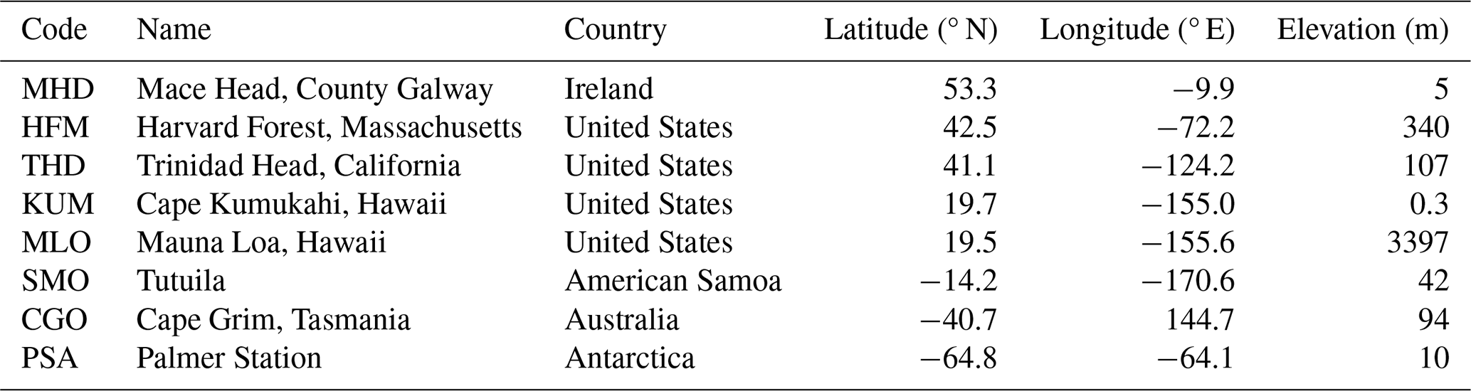
Flask measurements made by the NOAA-ESRL network are used in this work as a comparison with OCS total columns retrieved from IASI measurements. Ambient air is collected in flasks from 14 measurement sites and sent for analysis at the NOAA-ESRL Boulder Laboratories and analysed using gas chromatography and mass spectrometry methods to estimate mixing ratios of OCS (Montzka et al., 2007). The majority of the measurement sites are in the Northern Hemisphere (NH), especially North America, with none in regions of tropical rainforest. These data have been used in other work to validate modelled OCS concentrations (Suntharalingam et al., 2008; Berry et al., 2013; Cartwright et al., 2023) and have been assimilated into inversions schemes by Ma et al. (2021, 2024) and Remaud et al. (2022). A subset of the NOAA-ESRL flask data is used here, where monthly mean mixing ratios for 2018 from only those measurement sites within close proximity to coastlines are used, determined by sites that sit in or adjacent to a TOMCAT ocean grid cell, as we also compare the seasonal cycle of OCS_OCE with TOMCAT total columns. The furthest inland site is Harvard Forest, at approximately 100 km east from the North Atlantic coast. Table 1 provides information for the eight sites selected for comparison.

Table 1 NOAA-ESRL flask sampling site information for OCS measurements made at 8 sites. These sites are selected due to their proximity to an oceanic body.

2.1.4 Infrared atmospheric sounding interferometer instruments

The Meteorological Operational satellite (MetOp) programme, devised by the European Space Agency (ESA) and the EUropean organisation for the exploitation of METeorological SATellites (EUMETSAT), consists of three polar-orbiting satellites that provide accessible meteorological and climate data. MetOp-A, launched in October 2006, was the first European polar-orbiting satellite dedicated to operational meteorology. Although decommissioned in November 2021, during the majority of its lifetime MetOp-A provided almost global daily pole-to-pole coverage and orbited at an altitude of approximately 817 km and a 98.7° inclination angle to the equator, with an equatorial crossing time of 09:30 LT on a descending orbit (Clerbaux et al., 2009). Metop-B and MetOp-C were launched in September 2012 and November 2018, respectively. The equatorial crossing time for each is also 09:30 LT on the descending node. Metop-B and MetOp-C orbit 45 min apart with identical orbiting characteristics (prior to June 2017) – including twice daily global coverage on a repeat cycle of 29 d or 412 orbits. The MetOp series of satellites ensures a long-term reliable data source and provides redundancy in the system in case of a single instrument failure.

Each MetOp satellite contains an IASI instrument. Operating in a nadir-viewing configuration, IASI measures top-of-atmosphere radiation emitted from the Earth's atmosphere and surface at a moderately high spectral resolution of 0.5 cm⁻¹ over the over the range 645 to 2760 cm⁻¹. Each spectrum is sampled every 0.25 cm⁻¹ wavenumbers, yielding 8461 radiance channels (Clerbaux et al., 2009). These radiances can be used to derive a range of atmospheric trace gases, including OCS (Clerbaux et al., 2009; Camy-Peyret et al., 2017). The viewing configuration of IASI is that of a “whisk-broom” action, perpendicular to the direction of velocity. The total swath is approximately 2200 km (1100 km each side of the satellite), up to a maximum angle of ±48.3° with respect to the nadir. Each scan captures 30 instantaneous fields of view (IFOV), made up of a 2×2 matrix of 4 unique pixels, with a footprint diameter of 12 km at nadir extending to 39 km at the swath edge. Each satellite orbits Earth up to fifteen times a day, producing approximately 1.3 million spectral readings. The network of MetOp satellites can provide an extremely valuable tool in observing OCS concentrations on a daily, seasonal, or even annual basis.

Radiometric noise for each channel is quantified independently and was delivered to us directly from EUMETSAT, via Centre national d'études spatiales (CNES), and no additional inflation has been applied. The measurements made by the IASI instruments contain quantifiable random noise which is relatively low, approximately <2 $\mathrm{nW}{\mathrm{cm}}^{-\mathrm{2}}{\mathrm{sr}}^{-\mathrm{1}}$, in the spectral range used to retrieve OCS columns (2000 to 2100 cm⁻¹). Vincent and Dudhia (2017b) show that the signal of OCS absorption is above the noise level of IASI between 2040 and 2080 cm⁻¹ in a scene with background OCS (404 ppt). In addition, we see in Fig. S1 in the Supplement that a tropospheric concentration of around 100 ppt (and total column amount of 2.1×10¹⁵ molecules cm⁻²) would yield a detectable signal of OCS, as most of the P and R branches are above the instrument noise. The profiles used for this test are shown in Fig. S2, where we compare simulated IASI measurement spectra with and without OCS, using the RFM, then compare the residual spectra. This detection capability is well below the tropospheric values of OCS we see in satellite, surface observations and models (Montzka et al., 2007; Barkley et al., 2008; Glatthor et al., 2017; Bernath et al., 2020; Cartwright et al., 2023).

2.2 Retrieval methodology

2.2.1 ULIRS

ULIRS is based on the optimal estimation method, as explained by Rodgers (2000). The forward model, F, is the physical representation of the forward function, the mathematical operation relating the measurements, y, to the true atmospheric state x, and can be written as:

$$\begin{array}{}\text{(1)}& \mathit{y}=\mathrm{F}(\mathit{x},\mathit{b})+\mathit{ϵ},\end{array}$$

where the measurements, y, are top of atmosphere IASI radiances, x is the state vector, containing all retrieved parameters (OCS, CO₂, H₂O, temperature profiles and surface temperature), b represents the atmospheric parameters not included in the state vector (CO, O₃, CH₄), and ϵ represents uncertainties in the measurement and retrieval process. ULIRS uses the Reference Forward Model (RFM), a line-by-line atmospheric radiative transfer model, to simulate the IASI radiances (Dudhia, 2017). Profiles of CO, O₃, and CH₄ were included in fitting the modelled spectra, i.e. in b, but their contributions were not adjusted. Oceanic emissivity was assumed to be 0.98 (Seemann et al., 2008). For RFM calculations, we used look-up tables (LUTs) for H₂O, CO, O₃, and CH₄, pre-calculated by Vincent and Dudhia (2017a), as the use of LUTs improves the speed of RFM calculations by a factor of ∼20. For the CO₂ spectroscopic data, LUTs based on the Voigt lineshape with line mixing calculated using the HITRAN 2016 line-mixing package were used (Lamouroux et al., 2015; Gordon et al., 2017). For OCS, the HITRAN 2016 linelist was used directly for more precise computation of the contribution of OCS to the absorption spectra (Gordon et al., 2017).

The strongest absorption of OCS in the IR occurs over the range 2000–2100 cm⁻¹. Figure 1 presents an example spectrum calculated using the RFM for a pixel over the Indian Ocean, showing the contributions of OCS, H₂O, CO₂, O₃ and CO to absorbing upwelling infrared radiation. Note that the individual lines of OCS are not resolved when radiative transfer is modelled at a spectral sampling of 0.25 cm⁻¹. The ULIRS microwindows were selected by removing spectral points influenced by strong water features, which are associated with large residuals due to the inadequacy of the Voigt lineshape profile, and the strong CO₂ Q branch, which exhibits strong line mixing. Hence, the P branch of the ν3 band of OCS (below 2062 cm⁻¹) is the region of most interest for providing OCS information. The final microwindow set is shown graphically in Fig. 2 for a spectrum over the Indian Ocean.

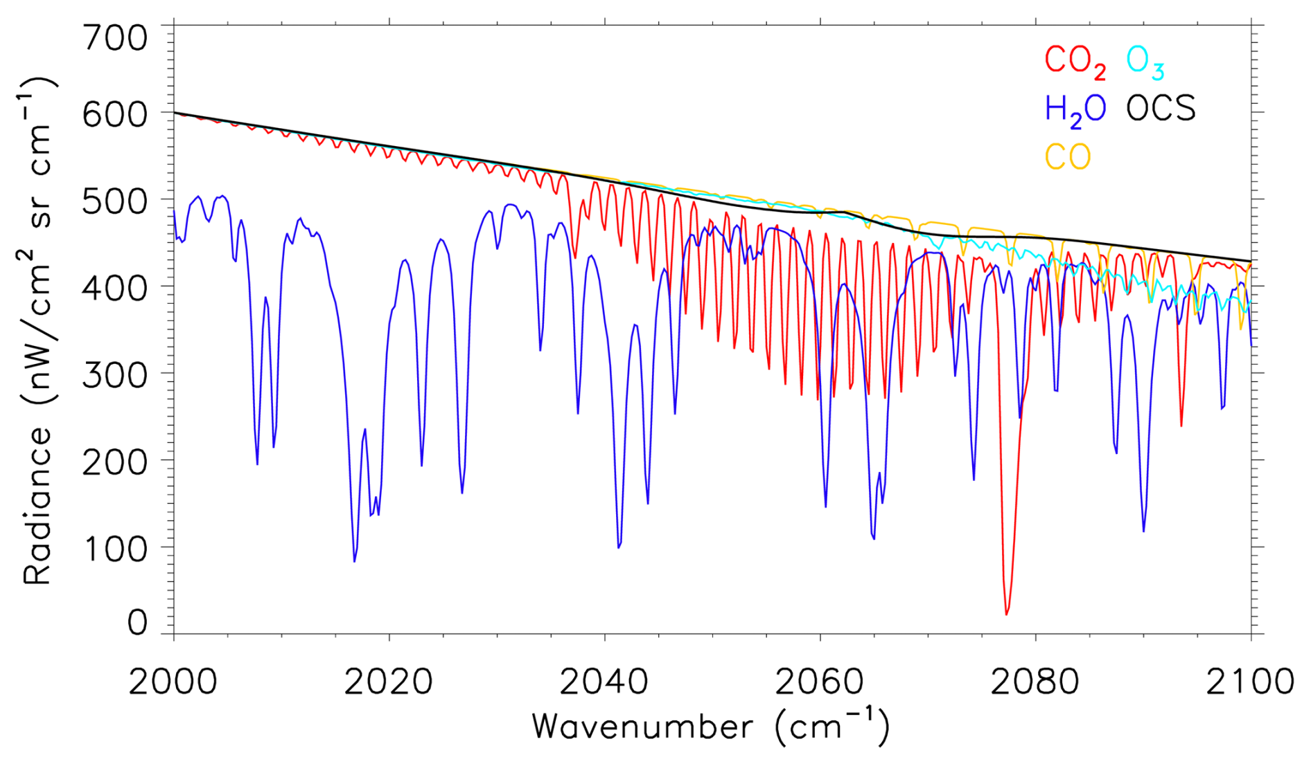
Figure 1 Modelled top-of-atmosphere radiances ($\mathrm{nW}{\mathrm{cm}}^{-\mathrm{2}}\mathrm{sr}{\mathrm{cm}}^{-\mathrm{1}}$) showing absorption contribution from all five species in the full range considered for OCS microwindow selection: 2000–2100 cm⁻¹, for a pixel in the Indian Ocean (0.05° S, 67.6° E) on the 18 July 2018. A spectral sampling of 0.25 cm⁻¹ was used.

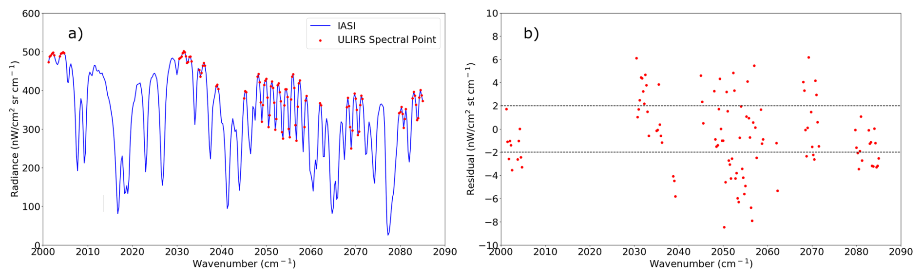
Figure 2 (a) IASI-B measurement spectra (blue), overlaid with ULIRS spectral points (red) and (b) ULIRS OCS retrieval residual spectra (red) for a test pixel over the Indian Ocean on the 18 July 2018: (0.05° S, 67.6° E). Mean residual = 2.59 $\mathrm{nW}{\mathrm{cm}}^{-\mathrm{2}}\mathrm{sr}{\mathrm{cm}}^{-\mathrm{1}}$. The grey lines indicate the ±2 nW noise estimate for this spectral region.

EUMETSAT Level 2 temperature, H₂O, CO, and O₃ data were used as the a priori for these species. For CO₂, a stand-alone a priori profile generation tool designed for the Total Carbon Column Observing Network (TCCON) (Toon and Wunch, 2015) (GGG2014 release) was used as prior information. A reference atmospheric profile was used for CH₄ (Remedios et al., 2007). The a priori profiles of OCS were created in 10° latitude bins by stitching together a homogeneous tropospheric profile concentration of 480 ppt from the surface to the tropopause with ACE-FTS stratospheric profiles averaged between 2004 and 2020, and an upper stratospheric value of 1 ppt. The value of 480 ppt is based on tropospheric values measured by ACE-FTS (Barkley et al., 2008), surface observations (Montzka et al., 2007) and model simulations (Cartwright et al., 2023). The troposphere and ACE-FTS profiles were stitched together and smoothed using a weighting function 2 km either side of the estimated tropopause height in 1 km increments. The final OCS a priori profiles are plotted in Fig. 3.

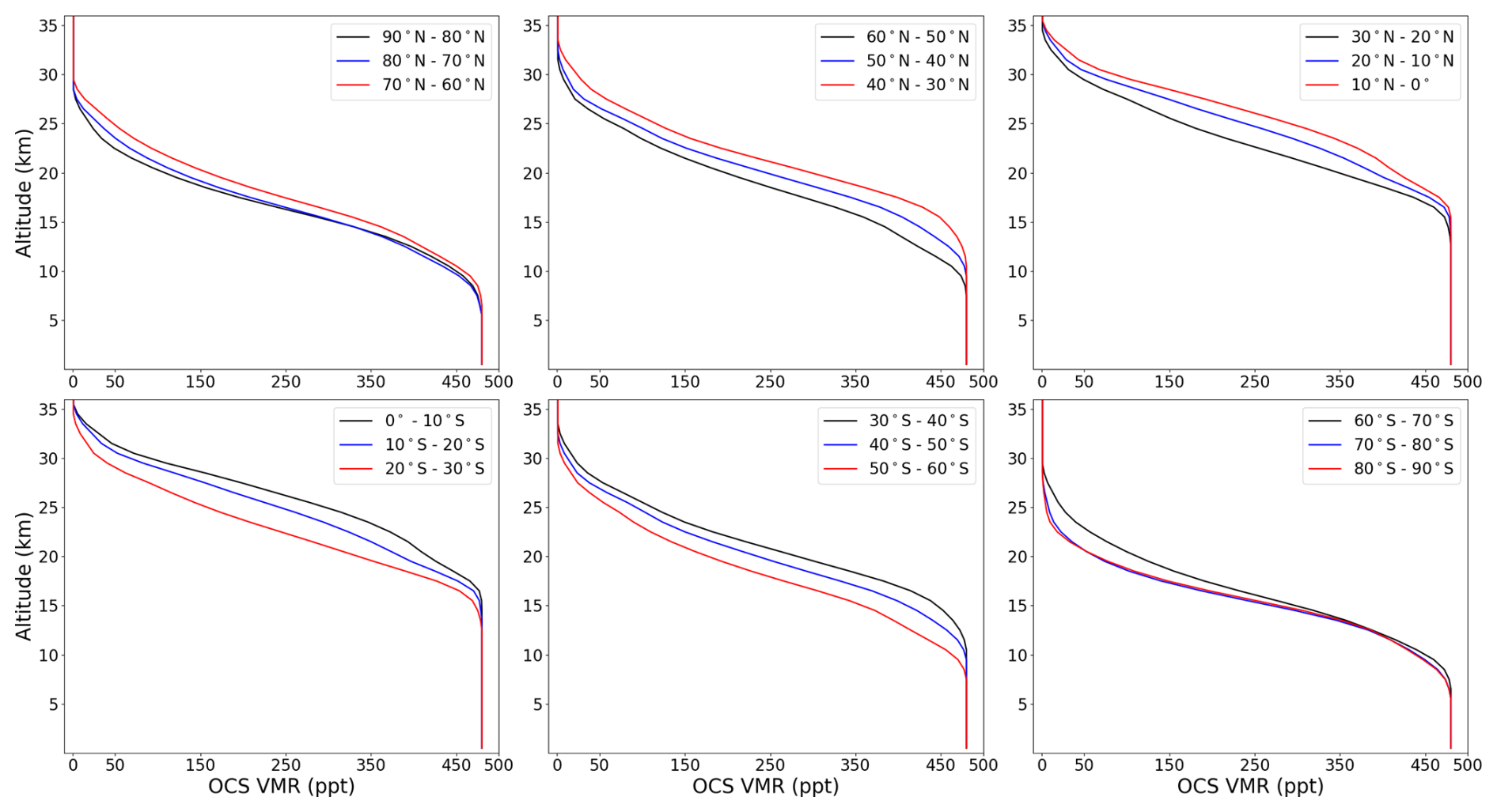
Figure 3 ULIRS a priori profiles of OCS (ppt) derived from ACE-FTS OCS averaged between 2004 and 2020 in 10° latitude bins, stitched to a tropospheric concentration of 480 ppt and an upper stratospheric value of 1 ppt.

The OCS retrieval grid is a 31-layer altitude grid from the surface to 31 km in equal increments with an additional single upper layer between 31 and 50 km, over the oceans this yields layers of 1 km thickness below 31 km. Using a single upper stratospheric layer, above 31 km, does not impact the outcome of the retrieval significantly but does reduce computational expense, due to the relatively low OCS concentration. To resolve the height above sea level for in-land water pixels, we use a Digital Elevation Model (DEM) that determines global surface elevation on a 30 arcsec-spaced grid (approximately 1 km), developed by the United States Geological Survey (USGS, 2017). The retrieval grid floats above the topography of the surface and the layer widths will therefore vary depending on the lower-most altitude, for example, if the surface of the pixel is 3.1 km above sea level, the layer widths would be 0.9 km, rather than 1 km.

Uncertainty in the a priori is quantified via the a priori covariance matrix, S_a. An a priori covariance matrix is defined for all layers of the state vector, except for the surface temperature which is assigned a covariance of 0.0025 K². As surface temperature utilises the IASI L2 product, trust in the surface temperature estimate is high and therefore the covariance is kept low so not to change the surface temperature significantly in the retrieval. Diagonal elements of the covariance matrix are defined as the variance (the square of the standard deviation) and are quantified as a percentage of the a priori mixing ratio at each altitude, namely 40 % for OCS, 20 % for water vapour, 2.5 % for CO₂, with a constant value of 1 K used for temperature. Off-diagonal elements of the covariances are calculated using the Gauss-Markov equation (Eq. 2.83 in Rodgers, 2000):

$$\begin{array}{}\text{(2)}& {\mathbf{S}}_{ij}=\sqrt{{\mathbf{S}}_{ii}{\mathbf{S}}_{jj}}\exp \left({\displaystyle \frac{-(z_i-z_j{)}^{\mathrm{2}}}{z_{\mathrm{s}}^{\mathrm{2}}}}\right),\end{array}$$

where S_ij denotes the covariance in the diagonal of the ith and jth element (representing retrieval levels), and z is the corresponding altitude. A smoothing length, z_s, of 7 km was employed for all off-diagonal calculations, due to the lack of fine structure in the constructed OCS a priori profiles.

In total, about 160 million measurements made between 70° S and 70° N latitude during 2018 over oceans and lakes by IASI instruments on MetOp-A and -B were processed. Observations were first filtered based on the operational Level 2 cloud flag (<10 % cloud) to remove any contaminated by cloud, before being passed to the ULIRS algorithm (August et al., 2012). This utilises the Levenberg-Marquardt iterative technique, where a “damping factor”, λ, is calculated after each iterative step to minimise a cost function (J),

$$\begin{array}{}\text{(3)}& J=(\mathit{y}-\mathrm{F}(\mathit{x}\left){)}^T{\mathbf{S}}_{\mathit{ϵ}}^{-\mathrm{1}}\right(\mathit{y}-\mathrm{F}\left(\mathit{x}\right))+(\mathit{x}-{\mathit{x}}_{\mathrm{a}}{)}^T{\mathbf{S}}_{\mathrm{a}}^{-\mathrm{1}}(\mathit{x}-{\mathit{x}}_{\mathrm{a}}).\end{array}$$

The first part of the right-hand-side is an error-weighted measure of the difference in model estimate and observations, where y is the measurement, F(x) the fitted modelled radiance and S_ϵ the covariance matrix containing error in the measurement. The second part quantifies the amount the state vector, x, can and should deviate from the prior approximations, x_a, weighted by the a priori covariance matrix in Eq. (2) , S_a.

The damping factor is used in the calculation of the state vector, according to

$$\begin{array}{}\text{(4)}& \begin{array}{rl}{\mathit{x}}_{i+\mathrm{1}}& ={\mathit{x}}_i+\left(\right[\mathrm{1}+\mathit{\lambda }]{\mathbf{S}}_{\mathrm{a}}^{-\mathrm{1}}+{\mathbf{K}}_i^T{\mathbf{S}}_y^{-\mathrm{1}}{\mathbf{K}}_i{)}^{-\mathrm{1}}\\ & \times \left[{\mathbf{K}}_i^T{\mathbf{S}}_y^{-\mathrm{1}}\right(\mathit{y}-\mathrm{F}\left({\mathit{x}}_i\right))-{\mathbf{S}}_{\mathrm{a}}^{-\mathrm{1}}({\mathit{x}}_i-{\mathit{x}}_{\mathrm{a}}\left)\right].\end{array}\end{array}$$

As outlined by Ceccherini and Ridolfi (2010), λ is initialised to a value of 0.1, and if the cost function is larger than in the previous step, λ is increased by a factor of 8, but if it is less, λ is reduced by a factor of 4. In Eq. (4) K are the Jacobians, which provide an indication of the sensitivity of the forward model to the state vector, referred to as a Jacobian as it is a matrix of derivatives. In addition to simulating top-of-atmosphere radiation, Jacobians are also calculated by the RFM, using a factor of 1 % perturbation for all trace gases included in the state vector and 1 K for temperature.

ULIRS applies two criteria: firstly, the retrieval is limited to 30 iterations, although in practice this is rarely realised because the solution typically converges within 2 to 4 iterations, and secondly convergence is satisfied when the cost function lies within 0.01 of values for the previous iteration (Illingworth et al., 2011). A good quality convergence is considered to have been reached if χ²≈m, where we consider m is the first part of the right-hand-side of Eq. (3), normalised by the number of measurement channels (see Fig. 2a), referred to as the chi-squared test.

3 Retrieval outputs

3.1 Characterisation and error analysis

Spectral radiance measurements from the IASI instruments on MetOp-A (IASI-A) and MetOp-B (IASI-B) were used to retrieve OCS profiles over the oceans, which we convert into total columns, denoted OCS_OCE-A and OCS_OCE-B, respectively, and collectively referred to as OCS_OCE. The method of converting profiles into total columns is presented by Deeter (2002). We focus on pixels over water in this work to simplify the accounting of emissivity in the retrieval. Figure 4 shows typical OCS_OCE-B averaging kernels for two pixels selected from a small region over the Indian Ocean. Averaging kernels, denoted as A in Eq. (5), calculated at each retrieval level, allow us to quantify the sensitivity of the retrieved state vector, $\widehat{\mathit{x}}$, to the true state of the atmosphere, x,

$$\begin{array}{}\text{(5)}& \mathbf{A}={\displaystyle \frac{\partial \widehat{\mathit{x}}}{\partial \mathit{x}}}.\end{array}$$

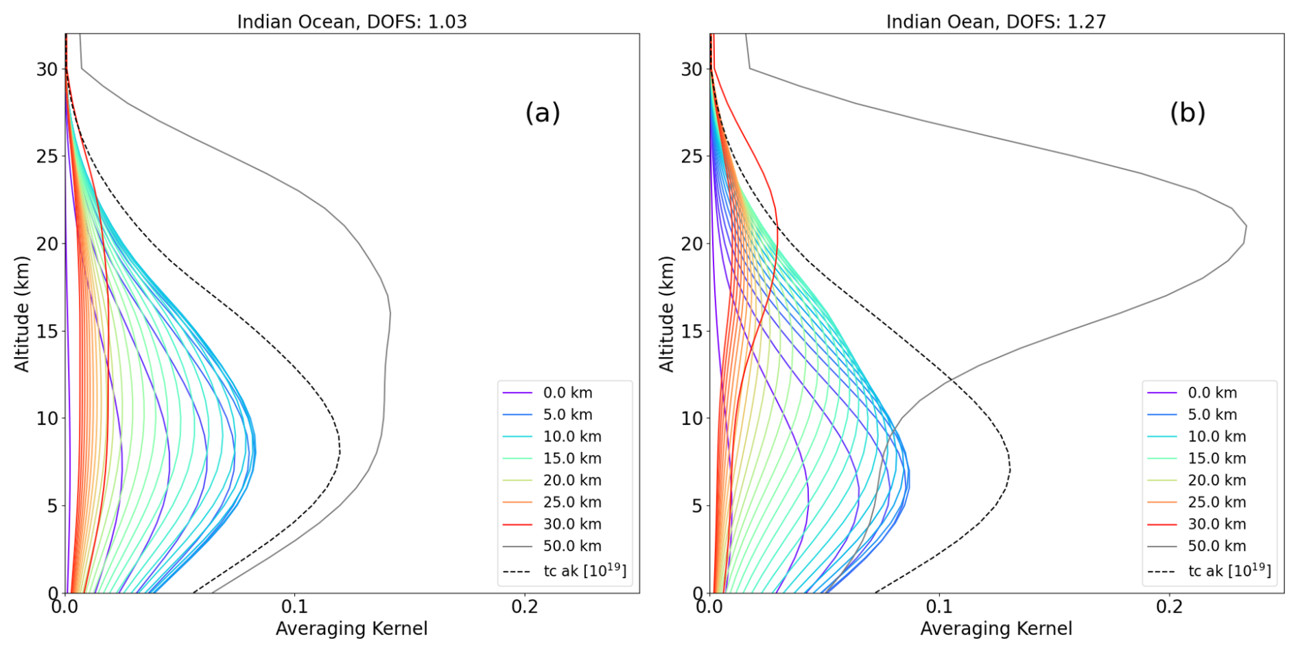
Figure 4 Averaging kernels (AKs) for each level of the ULIRS OCS retrieval grid for pixels over the Indian Ocean, illustrating (a) the minimum DOFS case (4.0° S, 66.8° E; DOFS=1.03) and (b) the maximum DOFS case (0.15° S, 64.1° E; DOFS=1.27). Coloured lines represent AKs at different retrieval grid levels; only every 5th level is labelled in the legend (e.g., “0.0 km” = surface, “5.0 km” = 5 km altitude level). The grey line indicated the top level (50 km), and the black dashed line shows the total column averaging kernel (tc_ak, units: $\mathrm{molecules}{\mathrm{cm}}^{-\mathrm{2}}{\mathrm{ppm}}^{-\mathrm{1}}$). Pixels were selected from daytime pixels for the period between 9 and 26 July 2018, from OCS_OCE-B measurements.

ULIRS employs a method of calculating A specifically for retrieval schemes utilising the Levenberg-Marquardt technique (Ceccherini and Ridolfi, 2010), where

$$\begin{array}{}\text{(6)}& \mathbf{A}=\mathbf{TK}.\end{array}$$

In Eq. (6), K represents a Jacobian, i.e. the sensitivity of the forward model to the state vector. T is a weighting term that factors in all iterative steps required for the scheme to converge, given by

$$\begin{array}{}\text{(7)}& {\mathbf{T}}_{i+\mathrm{1}}={\mathbf{G}}_i+(\mathbf{I}-{\mathbf{G}}_i{\mathbf{K}}_i-{\mathbf{M}}_i{\mathbf{S}}_{\mathrm{a}}^{-\mathrm{1}}){\mathbf{T}}_i,\end{array}$$

where i represents the ith iterative step of the retrieval, where T₀=0, I is the identity matrix, and M and G are given by

$$\begin{array}{}\text{(8)}& {\displaystyle }{\mathbf{M}}_i=({\mathbf{K}}_i^T{\mathbf{S}}_y^{-\mathrm{1}}{\mathbf{K}}_i+(\mathrm{1}+\mathit{\lambda }\left){\mathbf{S}}_{\mathrm{a}}^{-\mathrm{1}}\right),\text{(9)}& {\displaystyle }{\mathbf{G}}_i={\mathbf{M}}_i{\mathbf{K}}_i^T{\mathbf{S}}_y^{-\mathrm{1}}.\end{array}$$

This method replaces the use of a Gain matrix as proposed by Rodgers (2000). The information from the retrieval can be quantified by taking the trace of A, known as the degrees of freedom for the signal (DOFS). DOFS quantifies the number of independent pieces of information obtained from the measurement in the retrieval.

Figure 4 illustrates the averaging kernels (AKs; multi-colored lines in rainbow order) for two selected pixels within a grid box over the Indian Ocean ([4° S, 0°], [64° E, 68° E]). Each AK corresponds to a single retrieval level in the 31-level vertical grid. For clarity, the legend labels only every 5th level (e.g., “0.0 km” = surface level, “5.0 km” = 5 km level), but all levels are plotted. The total column averaging kernel (tc_ak; black dashed line) represents the integrated sensitivity across all levels, calculated using the same method as for the OCS total columns (see Deeter, 2002).

Figure 4a shows the sounding with the minimum DOFS (1.03), where the AKs peak toward the upper end of the sensitivity range, around 9 km, indicating that the retrieval provides just over one independent piece of information. Figure 4b shows the maximum DOFS case (1.27), with improved sensitivity in the mid-troposphere, around 6–7 km, and additional sensitivity in the upper troposphere and lower stratosphere between 17 and 22 km. The total column averaging kernel is scaled by 10¹⁹ (units: $\mathrm{molecules}{\mathrm{cm}}^{-\mathrm{2}}{\mathrm{ppm}}^{-\mathrm{1}}$) and, like the individual AKs, shows peak sensitivity in the mid-troposphere (6–9 km, ∼500–300 hPa).

Notably, the AKs peaking around 20 km correspond to retrieval levels above 30 km, indicating vertical displacement of sensitivity, i.e., due to poor measurement sensitivity higher up, the AKs shift the sensitivity to lower levels. This is evident in the grey line, corresponding to the AK for the top retrieval level (50 km), which shows relatively strong sensitivity due to the thickness of the layer below it (down to 30 km), enhancing the integrated signal.

Figure 5 shows seasonal mean χ² values (top), DOFs (middle), and sea surface temperature (SST, bottom) for 2018 from combined OCS_OCE-A and OCS_OCE-B retrievals. The χ² values are normalised by dividing by the number of measurements, m; a value of 1 shows an ideal fit of the model to the measurements. Traditionally this test is used to understand if the retrieval is both sensible and reliable, with a value larger (or smaller) than 1 indicating there are inadequacies in the retrieval, which can include the quality of the a priori and spectroscopic information provided in the forward model. While there are some seasonal patterns in χ² from the retrievals, much of the ocean is between 3 and 5. We see visually that there is a correlation between χ² and SST (hence the value in much of the tropics exceeds 4). As χ² is inherently linked to the quality of the retrieval and convergence, one might expect variations in χ² to have some kind of correlation (or inverse correlation) with elements in the state vector, however this does not translate into a bias in the retrieved OCS total column amounts, which is a positive outcome. This is shown graphically in the Supplement: Fig. S3, for a random subset of 200 000 retrieved profiles from each season of OCS_OCE-B in 2018 (see titles). The large χ² values are likely linked to the inability to fit the IASI spectra within measurement noise, which is principally due to deficiencies in the spectroscopy, most notably not accounting adequately for non-Voigt lineshapes of CO₂.

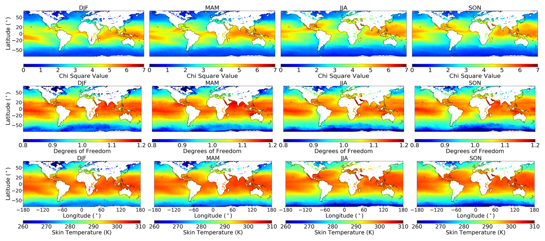
Figure 5 Top row shows χ², middle row shows mean DOFS, bottom row shows sea surface skin temperature (K). All rows are seasonal (identified in the title) and combine both day and night OCS_OCE retrievals from 2018, in 1°×1° bins.

As evidenced in Fig. 4, the DOFS are generally around 1, indicating that each retrieved profile provides approximately one piece of information for the OCS column. As shown in Fig. 5 DOFS are fractionally larger over the tropics, which is to be expected due to a stronger signal (Kuai et al., 2014).

Uncertainties in the retrieved parameters are defined using the linear error analysis approach presented by Rodgers (2000), except for the measurement error covariance, which is defined as

$$\begin{array}{}\text{(10)}& {\mathbf{S}}_{\mathrm{m}}={\mathbf{TS}}_y\mathbf{T},\end{array}$$

where T corresponds to the final iteration of Eq. (7), as outlined by Ceccherini and Ridolfi (2010).

Figure 6 presents the main retrieval error profiles for the same pixels used in the analysis of information content. The total retrieval error, also known as the a posteriori error, is the combined error contributions of S_m and the smoothing error, S_S,

$$\begin{array}{}\text{(11)}& {\mathbf{S}}_{\mathrm{S}}=(\mathbf{A}-\mathbf{I}){\mathbf{S}}_{\mathrm{a}}(\mathbf{A}-\mathbf{I}{)}^T.\end{array}$$

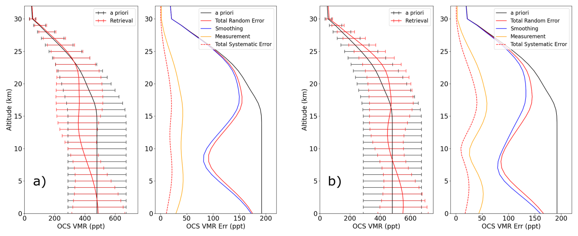
Figure 6 Profiles of retrieved and a priori OCS (left) and profiles of error components (right) for (a) minimum DOFS case and (b) maximum DOFS. The 2 pixels selected correspond to Fig. 4, where (a) Indian Ocean minimum DOFS: 4.0° S, 66.8° E and (b) Indian Ocean maximum DOFS: 0.15° S, 64.1° W.

As shown in Fig. 6, S_S is the major contributor to the error in all instances, resulting from the finite number of spectral measurements and atmospheric levels on which to retrieve information. Therefore, the error is mainly a consequence of the weakness and breadth of the OCS spectrum, such that the instrument spectral resolution cannot resolve the spectral features of OCS. Peaks in sensitivity in Fig. 4 are matched with troughs in the smoothing error in Fig. 6. This is also the case for S_m, the second largest contributor to the error, which is less important to the overall error below ∼18 km. Note also that DOFS are inversely correlated to retrieval error in the troposphere (below ∼15 km), hence we see a smaller error in Fig. 6b.

Figure 6 also presents the total systematic error, made up of the error contributions from the IASI instrumental line shape (ILS) error, radiometric stability (offset) error and radiometric accuracy (gain) error, as described by Illingworth et al. (2011). These individual contributions have been combined in quadrature, with the ILS error the major contributor to the total systematic error.

Retrieval error profiles are converted to columns using the same equations as for OCS_OCE (Deeter, 2002). Figure 7 presents global total column retrieval error for OCS_OCE, generally between approximately 2–3×10¹⁵ molecules cm⁻², corresponding to 18 %–38 % of the corresponding OCS total column amount, depending on location and time of year.

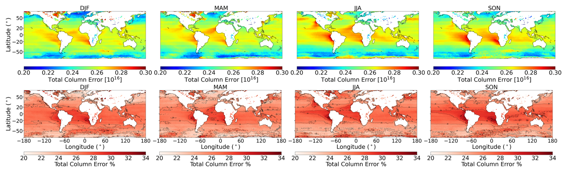
Figure 7 Seasonal mean OCS_OCE posterior error in units of molecules cm⁻² (top), for 2018, in 1°×1° bins. Percentage error relative to the total column amount is shown in the bottom row and the columns indicate DJF, MAM, JJA and SON respectively.

3.2 Total column estimate of OCS

OCS_OCE total column data were filtered to remove outliers, with criteria chosen to ensure robust retrieval quality and improve dataset stability for climatological applications rather than for detecting localized enhancements. Retrievals with DOFS<0.6 were excluded because the information content was substantially weighted towards the a priori, rather than the measurement (as explained in Sect. 3.1). Due to the presence of large normalized χ² values in the dataset, a conservative upper limit of 7 was adopted to reject retrievals with poor spectral fit or weak convergence. This value is based on retrieval characterisation and aligns with thresholds used in similar retrieval frameworks (e.g., Rodgers, 2000), in this case removes data more than (approximately) 3 standard deviations above the mean. This corresponds to the tail of the dataset's χ² distribution. The total column error threshold of $>\mathrm{4.0}\times {\mathrm{10}}^{\mathrm{15}}$ molecules cm⁻² was determined empirically by examining the error distribution and removing the extreme tail, which primarily consisted of retrievals with unrealistic variability. These filters removed approximately 2 % of the total number of pixels retrieved.

Additionally, data at the edges of swaths (above a satellite zenith angle of 48°) are removed due to artificial inflation of OCS total columns, caused by the intersection of a larger airmass, relative to a nadir view, as has been done in other work (Vincent and Dudhia, 2017b). Monthly mean OCS_OCE total columns for day and night are presented in Fig. 8, in 1°×1° bins over the oceans and lakes for 2018. After quality and cloud filtering, there are ∼6–7 million retrieved pixels per satellite each month.

Figure 8 Monthly OCS_OCE total column in units of molecules cm⁻². Day and night are presented for each month of 2018, in 1°×1° bins. 2 months are presented on each row, with day and night split into separate columns.

Figure 8 shows the differences in spatial patterns exhibited by OCS_OCE between daytime and nighttime for each month in 2018. Between 50° S and 50° N, total column amounts in the daytime are about 2 % higher than nighttime (Figs. S4 and S5). While this does not show a correlation with diurnal variation in SST (Figs. S6 and S7), the larger total columns during the morning overpass (daytime) can be owed in part to the stronger sensitivity to OCS arising from the larger thermal contrast at this time (and slightly enhanced infrared signal at the top-of-atmosphere, Figs. S8 and S9). There are also likely to be some atmospheric and surface factors, even biogenic. The largest day-night differences in OCS_OCE are located in the tropical Atlantic in October–December and just off the South American west coast in August–October, peaking around 8 % and localised to just a few 1°×1° grid cells.

The global peak in OCS_OCE occurs around April and May in the NH (Fig. 8). Daytime mean total columns are approximately 10.3 ± 0.27×10¹⁵ and 10.3 ± 0.31×10¹⁵ molecules cm⁻², respectively, for April and May between 20 and 60° N, and 9.96 ± 0.23×10¹⁵ and 9.96 ± 0.21×10¹⁵ molecules cm⁻² for the respective months in the corresponding Southern Hemisphere (SH) latitude band. Similar diurnal differences are observed in MIPAS at 10 km for the same months between 2008 and 2012 (Glatthor et al., 2017). The NH peak in OCS_OCE slightly lags behind the start of the NH growing season due to the lag of surface processes influencing its concentration in the free troposphere, i.e. advection of OCS poor airmasses; a similar behaviour is also shown in TOMCAT OCS model simulations and ACE-FTS observations (Cartwright et al., 2023). The build-up of atmospheric OCS, peaking in April and May, results from global surface emissions (mainly oceanic and anthropogenic) exceeding surface sinks in the NH winter period.

Off the coast of eastern China and surrounding the Korean peninsula is a region of large total column OCS throughout much of the year, which is more obvious in November–February (see Fig. 8). Compared to the Pacific Ocean, the OCS columns are consistently around 10 % larger in the region between mainland China and Japan, ranging from a peak of 13.5×10¹⁵ to 14.3×10¹⁵ molecules cm⁻² in February and November, respectively. This peak in OCS_OCE coincides with a regional maximum in year-round anthropogenic emissions originating from Eastern China nearby (Zumkehr et al., 2018). Anthropogenic OCS emissions generally tend to be aseasonal, so the absence of this enhancement between July and October suggests a summertime peak in NH OCS removal (via photosynthesis, soil uptake and reaction with OH, all of which are proportional to incident solar radiation). Vincent and Dudhia (2017b) show similar spatial features in IASI OCS total columns and hypothesised the same origin.

OCS_OCE in the NH peaks around local spring time, which coincides with the maximum in NH oceanic emissions (Lennartz et al., 2021) and the minimum biosphere uptake. Emissions from far northern ocean (>66° N) generally peak in April, and those in the latitude band 23–66° N a month later in May. This pattern has been shown to be consistent interannually, with some underlying variation in the magnitude of these respective fluxes (Lennartz et al., 2021). These patterns are influenced by the global oceanic distribution of CDOM, which dictates the rate of emission (Lennartz et al., 2017). It is likely there is also contribution from the advection over the oceans of land processes (biosphere uptake and anthropogenic emissions), which can be hard to quantify and differentiate from oceanic emissions without the use of a model. The NH latitudinal distribution of elevated OCS_OCE, peaking around 40° N in May, resembles that of patterns observed by MIPAS and IASI (Glatthor et al., 2017; Vincent and Dudhia, 2017b), as well as in posterior model estimates in inversion modelling studies that assimilate surface observations (Ma et al., 2021; Remaud et al., 2022).

The OCS observations in Fig. 8, over the same latitude bands defined above, i.e. between 20 and 60°, show that the mean monthly NH OCS_OCE peaks in April (10.3 ± 0.27×10¹⁵ molecules cm⁻²) with a minimum in October (9.85 ± 0.28×10¹⁵ molecules cm⁻²), yielding a seasonal cycle amplitude of 0.49×10¹⁵ molecules cm⁻². For the SH, the observed seasonal cycle is weaker, with a maximum in March (9.96 ± 0.25×10¹⁵ molecules cm⁻²) and a minimum in October (9.81 ± 0.22×10¹⁵ molecules cm⁻²), yielding a seasonal cycle amplitude of just 0.15×10¹⁵ molecules cm⁻². It should be noted that there are large regions around Antarctica that might be due to artefacts in the retrieval (discussed in more detail below – see Fig. 9).

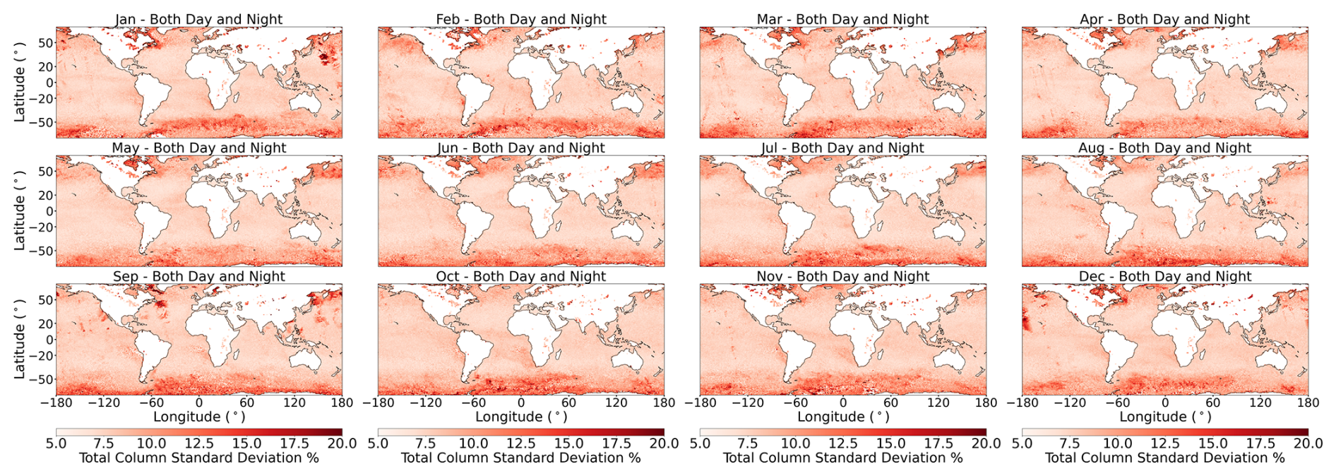
Figure 9 Monthly standard deviation (%) of total column OCS mean values for 2018. Day and night are combined for each month, in 1°×1° bins.

Regions of depletion of OCS_OCE can be observed in Fig. 8 throughout most of the year in the tropical Atlantic Ocean and eastern Pacific regions, between Africa and South America. Furthermore, a more seasonal longitudinal feature in OCS_OCE is also seen across much of the Pacific in the latter half of the year; this will be discussed shortly. The region of depletion in the tropical Atlantic has been hypothesised, detected and modelled by other studies (Berry et al., 2013; Glatthor et al., 2015; Vincent and Dudhia, 2017b; Ma et al., 2021; Remaud et al., 2022), where a depletion of approximately 5 %–15 % relative to surrounding ocean is to be expected. This Atlantic feature is predominantly attributed to strong terrestrial uptake over central Africa and advection of these OCS depleted airmasses (Glatthor et al., 2015; Ma et al., 2021; Remaud et al., 2022).

While these depletion features are visible throughout much of the year, they are less prevalent during JJA, which is slightly earlier than the peak in the African or Brazilian biomass burning seasons (Duncan et al., 2003). This suggests oceanic emissions are driving an increase in OCS at this time, as this is the period when depletion is expected to increase relative to May, as the growing season is very active in June and July. Fundamentally, Overall, the region of depletion is most likely attributed to strong surface vegetative uptake, potentially also to a weaker oceanic source. As many studies highlight, there is a need for surface-based tropical measurements of OCS, which could significantly improve validation of satellite products and models alike (Whelan et al., 2018; Ma et al., 2021; Remaud et al., 2022).

Another feature, predominantly in the latter half of the year (July–December), is the region of depletion throughout the northern tropical Pacific (around 0–10° N and 120° E–100° W). Vincent and Dudhia, (2017b) show a similar, albeit weaker, feature throughout the Pacific in their IASI total columns for 2014. This region has a peak daytime monthly mean of 10.1 ± 0.12×10¹⁵ molecules cm⁻² in April, before declining in May and beyond, reaching a minimum in September of 9.35 ± 0.16×10¹⁵ molecules cm⁻². This seasonal cycle is larger than that identified for the NH extra-tropical ocean region discussed previously. The spatial distribution of annual mean surface ocean concentration modelled by Lennartz et al. (2017) resembles that observed in OCS_OCE, such that the tropics are characterised by low sea surface ocean concentrations. Given the seasonality of the NH Pacific, it can be inferred that there is likely some contribution from the NH growing season, but further investigation using OCS_OCE in an inversion scheme would be essential to discriminate the origin of the sources and sinks dictating the behaviour in the Pacific.

The combined day-night monthly standard deviation of OCS_OCE is presented in Fig. 9, providing an indication of the monthly spread of OCS values. Between 40° S and 40° N the standard deviation rarely exceeds 10 %, with the exception of some anomalous regions in January and December around the Pacific and September over both the Atlantic and Pacific, which are likely artefacts of the retrieval. Overall, this variation is attributed to the natural variability in atmospheric OCS, rather than instrument noise (as the mean of so many data points have been taken) and retrieval errors. Figure 7 shows total column error in OCS_OCE with very little correlation between regions of high standard deviation and high retrieval error. In fact, over the Southern Ocean there appears to be an inverse correlation, where low errors are matched with high standard deviation. Between 40 and 70° N the standard deviation consistently exceeds 10 % but generally does not exceed 15 %. A December to March elevation in the standard deviation is apparent over the Labrador Sea and Hudson Bay. A similar feature is observed around Antarctica in Fig. 9, including the southernmost part of the Southern Ocean, which shows a region dominated by retrieval artefacts where the standard deviation of the measurements is generally between 10 % and 20 %. Similar patterns were observed by Vincent and Dudhia (2017b), suggesting there is a clear inadequacy in estimating OCS in this region. Part of the issue is likely attributable to a high albedo associated with the presence of sea ice, especially as the standard deviation peaks between August and October where sea ice is at or near its maximum (Eayrs et al., 2019). This likely indicates that the elevated OCS_OCE values in the Hudson Bay area in Fig. 8 (January–February) are retrieval artefacts, rather than real enhancements, driven by surface characteristics and retrieval limitations.

Seasonal OCS_OCE-A and OCS_OCE-B total columns are presented in the left and middle columns of Fig. 10, respectively, showing a similar overall pattern. The relative percentage difference, $(\frac{{\text{OCS}}_{\text{OCE-B}}}{{\text{OCS}}_{\text{OCE-A}}}-\mathrm{1})\times \mathrm{100}$, is displayed in the right-hand column of Fig. 10. A systematic difference between OCS_OCE-A and OCS_OCE-B, of approximately 3 %, is seen globally with regional peaks >3 % (for example in the northern Pacific in DJF), where OCS_OCE-B is larger. This difference affects both day and night data equally, so unlikely to result from a difference in thermal contrast resulting from the difference in equatorial crossing times of MetOp-A and -B (approximately 1.5 h in 2018). It could be caused by systematic observation discrepancy between the satellites, but more investigation is necessary.

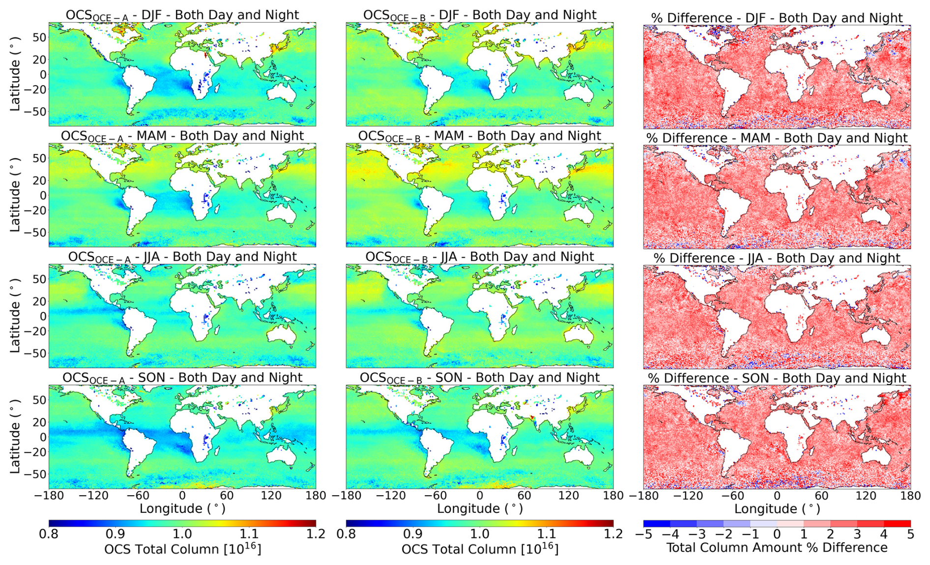
Figure 10 Seasonal estimates of total column OCS mean values in units of molecules cm⁻², for 2018, in 1°×1° bins. Left: OCS_OCE-A estimates, middle: OCS_OCE-B estimates, right: the % difference between OCS_OCE-A and OCS_OCE-B. Daytime and nighttime retrievals are combined.

There are no distinctive spatial patterns in the percentage difference in Fig. 10, although there are large and seemingly random aseasonal differences in the Southern Ocean, similar to those seen in the standard deviation of OCS_OCE in Fig. 9. This implies an artefact of the surface conditions is present, e.g. the presence of sea ice, rather than instrument noise or systematic retrieval bias (for this region exclusively).

4 Data comparison

4.1 TOMCAT model comparison

Retrieved OCS total columns (OCS_OCE) are compared with outputs of the TOMCAT 3-D off-line CTM (Cartwright et al., 2023). The model is driven here by ERA-Interim ECMWF meteorological reanalyses and an array of fluxes adapted from the literature (Berry et al., 2013; Kettle et al., 2002; Launois et al., 2015a; Suntharalingam et al., 2008; Zumkehr et al., 2018) or, in the case of vegetation, calculated using GPP fields from the JULES (Joint UK Land Environment Simulator) model (Slevin et al., 2016) and scaled to represent OCS uptake (Stimler et al., 2012; Cartwright et al., 2023). The period of 2004–2018 was simulated on a horizontal 2.8°×2.8° (T42) Gaussian grid and only 2018 is compared with the IASI measurements. TOMCAT OCS shows a reasonable comparison with ACE-FTS OCS profiles globally, agreeing to within ±25 ppt up to approximately 30 km. For further details the reader is directed to Cartwright et al. (2023).

OCS_OCE is shown in the top row of Fig. 11, which combines day and night retrievals. The middle row shows the TOMCAT model distribution with ULIRS averaging kernels applied (TOMCAT_AK), using:

$$\begin{array}{}\text{(12)}& {\mathit{x}}_{\text{TOMCAT\_AK}}={\mathit{x}}_{\mathrm{a}}+\mathit{A}({\mathit{x}}_{\text{TOMCAT}}-{\mathit{x}}_{\mathrm{a}}),\end{array}$$

where x_a is the a priori OCS profile, A contains the retrieval averaging kernels and x_TOMCAT is the model profile. We calculate profiles of TOMCAT_AK by applying the AKs from each OCS_OCE sounding to the respective monthly mean TOMCAT profile for the gridbox the sounding is in, after being interpolated onto the ULIRS retrieval grid. The TOMCAT_AK model profiles are then converted into total column amounts using the same calculation as for OCS_OCE total columns (Deeter, 2002) and a monthly mean is calculated. The difference between measurements and TOMCAT_AK is presented in the bottom row of Fig. 11. The model has previously been evaluated against independent measurements made by the ACE-FTS instrument above ∼5 km in altitude and against ground-based flask observations (Cartwright et al., 2023). However, there is still a region between the surface and ∼5 km of low sensitivity in the measurements and minimal evaluation in the model.

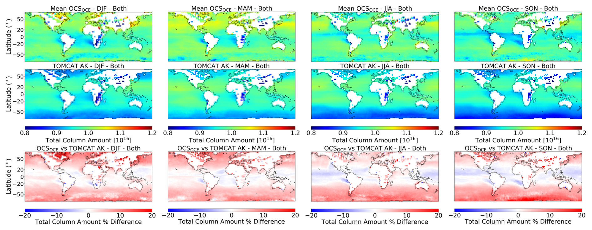
Figure 11 1st row: seasonal estimates of total column OCS_OCE mean values in units of molecules cm⁻², for 2018, in 1°×1° bins. 2nd row: TOMCAT OCS with OCS_OCE AK applied and 3rd row: the % difference with OCS_OCE.

Figure 11 shows that most of the tropics (defined as 30° S to 30° N for the purpose of this discussion) is similarly represented in OCS_OCE and TOMCAT, with differences around ±5 %, which is much smaller than satellite uncertainty. The model underestimates the zonal depletion in JJA and SON in places by between 5 % and 10 %, especially over the Pacific, which suggests surface OCS exchange is not well represented in the model. This area is dominated by oceanic emission with very little seasonality, but OCS_OCE suggests there is a seasonal variation in surface and atmospheric fluxes in this region. In contrast, TOMCAT exhibits seasonality in OCS total column amounts based on seasonal movement of the Inter-tropical Convergence Zone, as well as high latitude (HL) (approximately >50°) surface fluxes, i.e. there are large regions of depleted OCS in JJA and SON in the Southern Hemisphere high latitudes (SHHL), which can be attributed in part to a substantially lower tropopause height than in DJF and MAM. It has already been discussed that there is uncertainty in the retrievals in this region, so future work should be done to further validate the model simulations. An overestimation of the TOMCAT calculations in comparison with ACE-FTS profiles, in much of the mid-troposphere, of approximately 5 %–10 %, is seen by Cartwright et al. (2023), so OCS_OCE might well also be overestimating the SHHL, when compared with ACE-FTS observations. TOMCAT does a better job of representing the Northern Hemisphere mid latitudes (NHML) and Northern Hemisphere high latitudes (NHHL) compared with the SH. For JJA especially, there is excellent agreement (±5 %) north of 30° S. Once again, the NHHL region shows depletion in the model, which is not matched in OCS_OCE in DJF and MAM.

4.2 Ground-based observation comparison

To better understand how the seasonality of OCS_OCE compares with other OCS observations, OCS_OCE total column amounts are compared with surface flask observations (NOAA, US Department of Commerce, 2024). A comparison of OCS_OCE total columns with surface mixing ratios is presented in Fig. 12. OCS_OCE-A (grey) and OCS_OCE-B (red) retrievals are shown independently due to the difference in the two satellite observations, and TOMCAT total columns sampled over flask measurement sites are also shown (without AK applied, blue), for additional comparison. The calculations shown in Fig. 12 (R and P values) are with NOAA-ESRL observations for both OCS_OCE and TOMCAT. We do not apply averaging kernels to TOMCAT in this instance. OCS_OCE measurements are binned in the same spatial grid as TOMCAT (2.8°×2.8°) and monthly means of all profiles of OCS_OCE and TOMCAT within the closest grid box are shown. The error bars on NOAA-ESRL measurements (black) indicate the maximum and minimum measurements in the respective month, and the shaded area represents the standard deviation of the OCS_OCE-B observations. There are clear limitations in presenting this comparison, such as the column totals of OCS_OCE not representing the altitude at which the flask measurements are made, as well as misalignments in space and time when performing the co-location. Correlation coefficients, R, are shown for each site, as well as the associated P values – which quantify statistical significance, with a value of <0.05 providing evidence against a null hypothesis. A statistically significant correlation between OCS_OCE (or TOMCAT) and NOAA-ESRL surface observations can be seen at five of the eight sites.

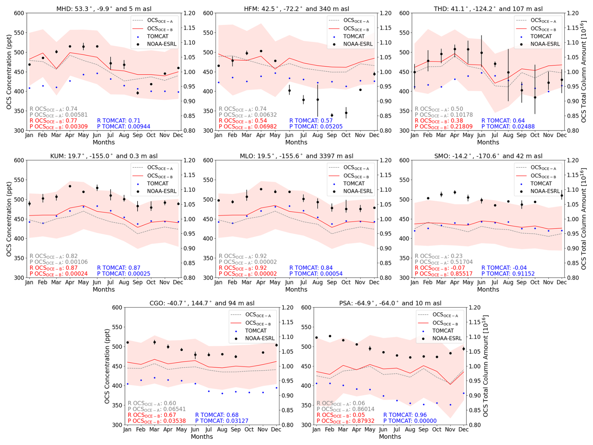
Figure 12 NOAA-ESRL surface flask monthly mean observations for 2018 (ppt, black circles) – left axis, are compared with OCS_OCE-A (grey dashed), OCS_OCE-B (red) and TOMCAT (blue) total column amounts (molecules cm⁻²) – right axis, for the same year. The shaded region represents standard deviation in OCS_OCE-B. Note the TOMCAT OCS total columns do not have IASI AKs applied and the statistical comparison is with NOAA-ESRL. All columns in the nearest TOMCAT 2.8°×2.8° grid box to the respective surface observations is used in the calculation of the monthly mean OCS_OCE-A, OCS_OCE-B and TOMCAT columns. Missing NOAA-ESRL points are due to missing data. Linear regression calculations of R represent the Pearson correlation coefficient and of P, the test for statistical significance in the relationship.

Mauna Loa (MLO) shows the best correlation of all eight sites for both OCS_OCE-A and OCS_OCE-B, with an R value of 0.92. This is a very important result, as MLO is not only a background measurement site, but is the highest altitude, at 3397 m, and therefore closest to the satellite measurement sensitivity range. Similarly, the results compare well with KUM, which uses the same OCS_OCE-A, OCS_OCE-B and TOMCAT profiles as for MLO, but measures at sea-level. The only other tropical measurement site is SMO, which shows a poor correlation in all three sets of data; the seasonality in flask measurements is not matched by the model or satellite datasets.

The NH sites MHD and HFM show a strong correlation between OSC_OCE and flask observations, around 0.7 (except OCS_OCE-B for HFM, which shows 0.54). Seasonality in OCS concentrations at the surface is characterised by a peak in June at MHD, followed by a substantial decrease in concentration as the NH growing season begins, reaching a minimum in September. The satellite observations capture the removal of OCS throughout the NH spring and summer period, as well as the build-up earlier in the year, unlike TOMCAT which shows an increase in OCS only around April. There is a noticeable drop in OCS total column amount in March 2018, which could potentially be driven by a significant shift in air mass direction, bringing air with less OCS abundance, however if this is meteorological in origin, one would expect a similar feature in the TOMCAT simulations. We suspect that the discrepancy in March is the main driver in reducing the correlation at MHD. HFM, while near the coast, is a forested site and therefore shows a larger seasonal cycle amplitude in the flask measurements, which is not seen in the satellite observations. This site shows an inconsistency between OCS_OCE-A and OCS_OCE-B retrievals (February and May are of note), the origin of which is uncertain. A lack of correlation at PSA is not surprising given the low DOFS (<0.8) at these latitudes and the systematically large standard deviations in this region (between 10 % and 20 %). The comparison at CGO, however, shows a statistically significant correlation of 0.67 for OCS_OCE-B, somewhat replicating the small seasonality in this region.

As highlighted by Serio et al. (2021), there are complications in characterising satellite observations by meteorology and airmass advection. They highlight that in the mid- and high- latitudes there could be a non-negligible impact from accounting for changing meteorological conditions on a seasonal basis, particularly over land. This is likely to have some impact on our results and in particular when comparing between total column amounts and surface observations, whereby the airmasses observed are substantially different.

5 Conclusions

An optimal estimation approach to retrieving OCS profiles from IASI radiance spectra has been presented using the ULIRS algorithm. Key features of the scheme include a state vector consisting of profiles of OCS, CO₂, H₂O and temperature, as well as surface temperature, on a 32-layer floating vertical grid, equidistant in altitude between the surface and 31 km, with a single additional layer up to 50 km, and a latitudinally varying a priori. Generally, the information content of the retrieved profiles exceeds 1 between ±50° latitude, peaking in the tropics where the thermal contrast is larger. The vertical sensitivity peaks around 6–10 km (500–300 hPa) in the troposphere. Retrieval errors in the total column amounts are 18 % to 38 %, generally peaking in the tropical regions. We see relatively large χ² values in the tropics of between 3 and 5, owed to inadequacies in the forward modelling. The use of Voigt line shapes in the current look-up tables is thought to be contributing to this.

The total column amounts over the global oceans, OCS_OCE, resemble spatial features seen in measurements and model estimates in other work, such as depletion in OCS over the tropical Atlantic (Berry et al., 2013; Glatthor et al., 2017; Vincent and Dudhia, 2017b; Ma et al., 2021) and can be linked to surface fluxes (Glatthor et al., 2015; Lennartz et al., 2017, 2021; Zumkehr et al., 2018; Cartwright et al., 2023), in this case biospheric uptake, which leads to smaller atmospheric OCS mixing ratios. OCS total columns display a seasonal amplitude of approximately 0.49×10¹⁵ molecules cm⁻² for the 20 and 60° N latitude band. For the corresponding band in the SH, this is approximately 0.15×10¹⁵ molecules cm⁻². Diurnal variations are limited to about ±2 %, with a positive bias toward daytime measurements owing to a larger thermal contrast. Additionally, there is a 3 % difference between MetOp-A and MetOp-B consistent globally, potentially owed to a systematic observation discrepancy between the two satellites.

Total column OCS_OCE agrees within ±5 % of modelled OCS using the TOMCAT model in the latitudinal band between 30° S and 30° N (Cartwright et al., 2023). Many of the spatial features in OCS_OCE are reflected in TOMCAT OCS, such as tropical Atlantic depletion and enhancement in the NH extra tropics. However, across much of the globe the model underestimates total column amounts compared to OCS_OCE by around 10 %, with the best agreement seen in the tropics, where the model tends to overestimate.

A comparison of OCS_OCE-B with coastal and island flask measurements yields good correlation (>0.67) at 5 of the 8 sites compared here. The best agreement is seen at Mauna Loa, Hawaii, with a correlation of 0.92. This is a particularly important result due to this station being the closest in altitude to that of the sensitivity satellite measurements. Future work should include a comparison between OCS_OCE and ground-based column observations from NDACC sites, including the application of IASI averaging kernels to NDACC profiles and vice versa.

Work is ongoing to extend the OCS_OCE dataset to multiple years (L1C radiance spectra are available between 2006–2021 from MetOp-A and 2012–present for MetOp-B) and potentially include retrievals from MetOp-C (2018–present). Prospective improvements to the retrieval scheme include implementing better spectroscopy in the RFM, especially for CO₂, and potentially other minor changes to the setup, such as the retrieval grid or prior covariances. Preliminary testing is ongoing for land-based retrievals of OCS from IASI measurement spectra, with a focus on tropical forest regions, provisionally with a spectrally-resolved emissivity product, but likely requiring retrieval of surface emissivity in the state vector, as has been done in other work (Camy-Peyret et al., 2017).

A strength of satellite observations compared to ground-based measurements is the spatial extent and resolution of the measurements and regularity of global coverage. We intend for OCS_OCE to be used in a formal flux inversion to better constrain surface OCS fluxes and provide better interpretation of global GPP. Furthermore, using ground-based datasets (NOAA-ESRL observations or NDACC profiles) to complement satellite observations, would not only allow for a better comparison between these datasets and OCS_OCE, but would open up possibilities for interpreting the spatial distribution of OCS_OCE in the context of surface fluxes.