Signatures of aerosol-cloud interactions in GiOcean: a coupled global reanalysis with two-moment cloud microphysics

Aerosols influence the Earth's radiative balance through direct interactions with radiation and by affecting cloud properties. Anthropogenic aerosols have led to cooling during the industrial era through aerosol–cloud interactions (ACI), including aerosol effects on cloud microphysical properties and the subsequent adjustments. However, large uncertainties remain in Earth system models (ESMs) regarding the magnitude of this cooling. In part, ESMs substantially disagree on cloud properties, thermodynamics, the hydrological cycle, and general circulation. Reanalysis provides a useful avenue for exploring the impact of ACI on clouds and radiation because its atmosphere is forced to match realistic conditions through the assimilation of observations. Here, we explore the impact of ACI on clouds in the GiOcean reanalysis – the first to incorporate aerosol-cloud interactions. We contrast variables important for ACI between GiOcean and satellite observations and develop 2-dimensional lookup tables of ACI for both using a source-sink budget perspective to attribute the changes in cloud droplet number (Nd) and liquid water path (LWP) to aerosol and meteorology. A compositing analysis using lookup tables shows that GiOcean captures key aspects of aerosol–cloud–precipitation interactions, including (1) activation of aerosol into cloud droplets, (2) effective precipitation scavenging of Nd, (3) suppression of precipitation by high Nd in regions with heavy aerosol emissions. In contrast, satellite observations do not exhibit clear patterns for processes (2) and (3). Random Forest analysis shows that interannual variability in Nd and LWP over the Northern Hemisphere ocean in GiOcean is primarily driven by precipitation, consistent with satellite observations.

1 Introduction

Climate change is driven by imbalances in Earth's energy budget, known as climate forcings, which result from changes in atmospheric composition (e.g., greenhouse gases, aerosols, ozone, stratospheric water vapor) and in surface properties such as surface albedo (Smith et al., 2021). Among these, the net effect of anthropogenic aerosols on Earth's energy budget (aerosol radiative forcing) remains one of the largest uncertainties in our projections of future warming (Bellouin et al., 2019; Watson-Parris and Smith, 2022). The change in reflected solar radiation due to anthropogenic emissions of aerosols (e.g., aerosol radiative forcing) is largely uncertain due to the complex effects that aerosols can have on climate (Bellouin et al., 2019). Aerosols affect the Earth's radiation balance in several ways. Aerosol alters the Earth's energy budget directly by scattering and absorption of radiation, termed aerosol-radiation interactions. Aerosol can affect climate indirectly through aerosol-cloud interactions (ACI) by (1) modifying cloud microphysical properties, and thereby altering cloud reflectivity, known as the Twomey effect (Twomey, 1977), and (2) by altering macrophysical properties induced by changes in cloud microphysics (Ackerman et al., 2004), such as cloud lifetime, precipitation formation and cloud cover. This effect is referred to as aerosol-cloud adjustments (Albrecht, 1989; Bretherton et al., 2007). The combined radiative forcing from the Twomey effect and aerosol-cloud adjustment is referred to as the effective radiative forcing due to ACI (Bellouin et al., 2019). ACI have led to cooling during the industrial era, but the degree to which ACI have affected the Earth's energy budget remains uncertain (Bellouin et al., 2019).

The uncertainty in ACI forcing arises not only from the understanding of the complexity of ACI processes, but also from how aerosols and clouds are represented in Earth system models (ESMs). Cloud microphysical processes are hard to represent in ESMs as these processes are small in scale (∼ µm), and ESMs (∼ 100 km) cannot resolve these small, fast processes dynamically (Liu and Kollias, 2023; Morrison et al., 2020), so parameterizations are necessary to describe these physical processes. Most ESMs use simplified “bulk” schemes (Morrison and Gettelman, 2008). One-moment schemes typically predict only the mass of hydrometeors and cannot capture aerosol-driven changes in droplet number or size, limiting their ability to simulate ACI. Two-moment schemes improve this by prognosing both mass and number concentrations, enabling explicit responses of cloud microphysics to aerosol perturbations (Twomey, 1977; Barahona et al., 2014). Many ESMs have implemented the two-moment microphysics scheme into cloud presentations and showed improved representation of cloud properties (Ghan et al., 1997; Lohmann et al., 1999; Ming et al., 2007; Barahona et al., 2014; Morrison and Gettelman, 2008).

Despite the advances in the representation of cloud microphysics in ESMs, the interaction of aerosol with clouds is always neglected in operational forecasting systems and climate reanalyses. In reanalyses that include an aerosol representation, a carefully crafted aerosol climatology is allowed to interact with radiation as a way of representing the aerosol direct effect; however, interactions with clouds are neglected (e.g., Bozzo et al., 2020). This approach has shown to improve the prediction of the African Easterly Jet (Tompkins et al., 2005) and tropical cyclogenesis (Reale et al., 2014). On the other hand, Zhang et al. (2016a) showed that numerical weather prediction (NWP) systems using aerosol climatologies overestimated surface temperature during a strong biomass burning event, whereas models with prognostic aerosols showed the correct surface cooling. In some cases the usage of aerosol climatologies may lead to degradation of the forecast skill, since without the feedback between aerosol and meteorology, anomaly centers associated with aerosol emissions become permanent, imprinting spurious temperature gradients that perturb global circulation (Morcrette et al., 2011). Ekman (2014) suggested that the explicit representation of ACI in ESMs improves the simulation of the historical surface temperature trend. This has been further shown during dust storms over Europe and North Africa where neglecting dust emissions and their effect on clouds can lead to overestimation of surface temperature in NWP (Bangert et al., 2012). Aerosol effects have been shown to play a significant role in the modulation of dust transport by the Madden Julian Oscillation (MJO) (Benedetti and Vitart, 2018) as well on hurricane development (Nowottnick et al., 2018). Given all of these potential interactions between aerosol and climate, there is a growing consensus that ACI must be represented in weather, seasonal forecasting models, and climate reanalyses (National Academies of Sciences, Engineering, and Medicine, 2016).

Furthermore, including a realistic representation of aerosols and clouds in reanalysis is particularly important given the strong spatial variability in aerosol radiative forcing, which can be can be either positive or negative depending on the region (Smith et al., 2021). Several factors contribute to such a heterogeneity. Aerosol have a shorter lifespan in the atmosphere than greenhouse gases, of the order of few days to about two weeks. Despite this, they may be transported around the globe and interact with clouds and radiation far away from their sources (Uno et al., 2009). Over this time their composition may change due to the interaction with local pollution sources and from oxidation processes. When aerosol particles reach pristine regions in the North Atlantic and the Pacific oceans, away from their emission sources, they may substantially impact the regional climate (Fan et al., 2016). Their emission rate changes over time, with marked seasonal cycles (McCoy et al., 2017; Kasibhatla et al., 1997), and long-term decadal trends (Bellucci et al., 2015; McCoy et al., 2018a). Volcanic events and even policy decisions (Yuan et al., 2024) add variability to the atmospheric aerosol concentration (Bellucci et al., 2015). It is known that over the time scale of days to months, aerosols have an observable, local effect on clouds and radiation (Fan et al., 2016; Breen et al., 2021). These effects can result in persistent radiative flux and cloud property anomalies, strong enough to modify large-scale atmospheric patterns (Morcrette et al., 2011; Bellucci et al., 2015; Ekman, 2012).

This study introduces a new coupled reanalysis dataset – GiOcean, which incorporates two-moment microphysics scheme for stratiform and convective clouds, enabling the explicit representation of ACI (Barahona et al., 2014; Molod et al., 2020). We focus on evaluating the impact of ACI in warm clouds by comparing it with observations of clouds, precipitation, and aerosol during periods of substantial emission changes over a multidecadal time scale.

2 Methods

2.1 The GiOcean Coupled Reanalysis

GiOcean is a global reanalysis dataset that spans from 1998 to the present, with a typical data availability lag of about six months due to the time required for quality control and data assimilation. GiOcean integrates three data assimilation systems for the atmosphere, aerosol, and ocean. These systems assimilate a vast array of observational data to calculate six-hourly “increments” that adjust meteorological, oceanic, and aerosol states, forcing the model to align with observations. Unlike typical reanalyses, which focus solely on meteorological states, GiOcean incorporates data from all three domains, providing a more comprehensive representation.

2.1.1 Modeling Description and Data Assimilation Approach

GiOcean is based on the Goddard Earth Observing System (GEOS) Subseasonal-to-Seasonal (GEOS-S2S) prediction system, developed by the Global Modeling and Assimilation Office (GMAO) (Molod et al., 2020). GEOS-S2S is a coupled Earth system modeling and data assimilation framework to produce forecasts on subseasonal to seasonal timescales. The core component of the GEOS-S2S system is the coupled Atmosphere-Ocean General Circulation Model (AOGCM). It includes atmosphere, land, aerosol, ocean, and sea ice components with spatial resolutions of approximately 50 km for the atmosphere and 25 km for the ocean. The atmosphere component of the GiOcean is the GEOS Atmospheric General Circulation Model (AGCM) (Molod et al., 2015; Rienecker et al., 2008). The ocean component of the GEOS AOGCM is the MOM5 (Modular Ocean Model version 5) ocean general circulation model (Griffies et al., 2005; Griffies, 2012), and the Community Ice CodE-4 sea ice model (Hunke, 2008). Ocean data assimilation follows the Local Ensemble Transform Kalman Filter approach (Penny et al., 2013). The land surface model uses a catchment-based approach and statistically represents subgrid-scale variability in surface moisture (Koster et al., 2000). To produce GiOcean, GEOS-S2S is retrospectively integrated starting on January 1998 using a time step of 450 s and assimilating atmospheric and ocean observations every six hours for the atmospheric and aerosol components and five days for the ocean, as described below.

The GiOcean reanalysis employs weak or “one-way” coupling, meaning that the ocean and aerosol components use a full assimilation system, while the atmosphere is “replayed” to a preexisting atmospheric reanalysis. In this approach, the atmospheric analysis increments used for model correction are derived from the pre-existing atmosphere-only reanalysis but adjusted for differences in model physics. This approach stabilizes the reanalysis by avoiding a full meteorological assimilation system, though it limits feedback between the ocean and atmosphere. GEOS-IT, produced for NASA's instrument teams, serves as a stable meteorological dataset for GiOcean (https://gmao.gsfc.nasa.gov/GMAO_products/GEOS-5_FP-IT_details.php, last access: 6 November 2025). Similar to the Modern-Era Retrospective Analysis for Research and Applications, Version 2 (MERRA-2) (Gelaro et al., 2017), GEOS-IT is a multidecadal retrospective reanalysis integrating both aerosol and meteorological observations (Gelaro et al., 2017; Randles et al., 2017). However, it incorporates recent model enhancements that provide more accurate representations of moisture, temperature, and land surfaces as well as the latest satellite observations through updated analysis techniques. While the atmosphere component of GEOS-S2S is “replayed” using the GEOS-IT reanalysis (Gelaro et al., 2017), the aerosol and ocean data assimilation systems, however, remain fully active.

2.1.2 Aerosols and Cloud Microphysics

Of significance to this work is that GiOcean explicitly assimilates aerosol fields. Furthermore cloud microphysics is described using a two-moment scheme, where cloud formation is linked to the aerosol concentration. This allows GiOcean to explicitly capture the aerosol direct and indirect effects.

Transport of aerosols and gaseous tracers such as CO are simulated using the Goddard Chemistry Aerosol and Radiation model (GOCART; Colarco et al., 2010). All components are coupled together using the Earth System Modeling Framework (Hill et al., 2004) and the Modeling Analysis and Prediction Layer interface layer (Suarez et al., 2007). GOCART is a mass-based aerosol transport model that explicitly calculates the transport and evolution of dust, black carbon, organic material, sea salt, and sulfate. To relate aerosol mass to number concentrations, prescribed size distributions were used to calculate mass-number conversion factors as detailed by Barahona et al. (2014). Dust and sea salt emissions are prognostic whereas sulfate and biomass burning data are prescribed (Randles et al., 2017). Volcanic SO₂ emissions are constrained by observations from the Ozone Monitoring Instrument (OMI) on-board NASA's EOS/Aura spacecraft (Carn et al., 2017).

Aerosol fields in GiOcean are assimilated using The Goddard Aerosol Assimilation System (GAAS) (Buchard et al., 2016). Aerosol assimilation is carried out in two steps. First the aerosol optical depth (AOD), is assimilated using the observations of AOD from multiple sources described in Table 2 of Randles et al. (2017), including the Multi-angle Imaging SpectroRadiometer (MISR), the Moderate Resolution Imaging Spectroradiometer (MODIS), the Aerosol Robotic Network (AERONET), etc. Then in a second step the analysis increment is distributed vertically and among the different aerosol species to update their mass mixing ratios. In GiOcean the overall assimilation cycle is controlled by the meteorology. The meteorological observing system (i.e., the collection of instruments, platforms, and networks that provide meteorological observations) is also much larger than the one used in GAAS (Gelaro et al., 2017). GAAS is used to assimilate aerosol fields in the MERRA-2 reanalysis, although the cloud microphysics scheme in MERRA-2 lacks a representation of the aerosol indirect effect.

In GiOcean a 2-moment cloud microphysics scheme is used to calculate the mixing ratio and number concentration of cloud droplets and ice crystals as prognostic variables for stratiform (i.e., stratocumulus, cirrus) and convective clouds (Barahona et al., 2014). Cloud droplet activation follows the approach of Abdul-Razzak and Ghan (2000). The stratiform cloud microphysics scheme follows Morrison and Gettelman (2008: MG08) with adjustments when incorporated into GiOcean (Barahona et al., 2014). The droplet autoconversion parameterization is replaced by the formulation of Liu et al. (2006). A parameterization of subgrid vertical velocity, which is important for particle activation, was developed and detailed in Barahona et al. (2014). MG08 is also modified to represent the impact of existing ice crystals on the development of cirrus clouds. Ice nucleation is estimated using a physically-based analytical approach (Barahona and Nenes, 2009) that includes homogeneous and heterogeneous ice nucleation, and their competition. The description of heterogeneous ice droplet formation by immersion freezing and contact ice nucleation follows Ullrich et al. (2017). Vertical velocity fluctuations are constrained by non-hydrostatic, high-resolution global simulations (Barahona et al., 2017). This configuration has been shown to reproduce the global distribution of clouds, radiation, and precipitation in agreement with satellite retrievals and in situ observations (Barahona et al., 2014; Molod et al., 2020).

2.2 Analysis method

2.2.1 Variables analyzed

This study focuses on the evaluation of ACI in warm clouds in GiOcean. We limit the scope to variables related to aerosol abundance, activation into cloud droplets, the state of cloud macrophysical properties, and precipitation rate. We focus on variables that can be compared relatively directly between GiOcean and spaceborne remote sensing, including aerosol optical depth (AOD), cloud droplet number concentration (Nd), liquid water path (LWP), and precipitation rate.

The aerosol metric we use is the AOD, which measures the column-integrated aerosol extinction (scattering and absorption of light) and is often related to the total amount of aerosols in the atmospheric column. Although AOD does not provide information for the vertical distribution of aerosols or the aerosol sizes and species in the column, AOD provides an estimate of column integrated aerosol loading nearly globally, with limitation at high latitudes due to snow contamination. This is in contrast to sparse in-situ observations of aerosols made by aircraft and surface sites, and can be compared relatively directly between models and observations.

The cloud microphysical property we evaluate in this study is Nd. Nd is key variable of state (or most important variable) in controlling ACI (Wood, 2012). Changes in Nd also alter cloud macrophysical properties (Ackerman et al., 2004, 2000; Albrecht, 1989; Bretherton et al., 2007).

The cloud macrophysical property we evaluate is liquid condensate mass. It provides a diagnostic of the liquid cloud adjustment to aerosol-induced changes in cloud microphysics (Bellouin et al., 2019; Song et al., 2024). In practice, liquid condensate mass is usually observed as column-integrated liquid water from remote sensing observations, which is known as liquid water path (LWP).

Nd and LWP have been shown to be very important variables in understanding the physical processes related to ACI (Mikkelsen et al., 2025; Gryspeerdt et al., 2019; Wall et al., 2022; Bellouin et al., 2019). While aerosol-driven changes in cloud microphysics and macrophysics are essential to ACI, they do not capture the full complexity of ACI processes. Precipitation drives coalescence-scavenging and depletes Nd (Wood et al., 2012; Kang et al., 2022; McCoy et al., 2020). Precipitation also serves as a proxy for moisture convergence and contains information about the large-scale environment, which in turn affects LWP (Mikkelsen et al., 2025). To evaluate how these variables are represented in GiOcean, we compare AOD, Nd, LWP, and precipitation rate from the GiOcean reanalysis with satellite observations, as detailed in Sect. 2.3.

2.2.2 Sensitivity metrics

In this study, we calculate two key sensitivity metrics. The sensitivity metric follows previous studies examining ACI (Ghan et al., 2016; Bellouin et al., 2019), as a way of evaluating the ACI presentation in GiOcean against satellite observations. The sensitivity of Nd to CCN represents the inferred efficacy of aerosol activation into cloud droplets and is expressed in Eq. (1).

$$\begin{array}{}\text{(1)}& S_{\text{Nd-AOD}}={\displaystyle \frac{\mathrm{d}\ln \mathrm{Nd}}{\mathrm{d}\ln \mathrm{AOD}}}\end{array}$$

Similarly, to quantify the extent of cloud macrophysical adjustments (e.g., changes in LWP) in response to microphysical perturbations, the sensitivity of LWP to Nd is calculated using Eq. (2).

$$\begin{array}{}\text{(2)}& S_{\text{LWP-Nd}}={\displaystyle \frac{\mathrm{d}\ln \mathrm{LWP}}{\mathrm{d}\ln \mathrm{Nd}}}\end{array}$$

We apply a consistent binning approach to compute these inferred sensitivities in both the GiOcean reanalysis and satellite observations. Monthly Nd is binned into 15 logarithmically spaced bins, and mean values of relevant variables (e.g., LWP, Nd, AOD) are calculated within each bin. Relationships between AOD and Nd, and between LWP and Nd, are then plotted using these bin-averaged values (Sect. 3.3). Logarithmic derivatives are then estimated using finite differences between the binned means. A weighted average of these derivatives is calculated, with weights corresponding to the number of data points in each bin. The binning approach smooths out random noise by enforcing 15 logarithmically spaced Nd bins, so that each derivative estimate is based on hundreds or thousands of observations and the resulting slopes (e.g., ln LWP versus ln Nd) are statistically robust and representative.

By comparing these metrics across GiOcean and satellite observations, we evaluate the representation of both aerosol activation and aerosol-cloud adjustment in the GiOcean reanalysis. The results are discussed in Sect. 3.3. We note that these inferred sensitivities (calculated from Eqs. 1 and 2) do not imply causation and may be strongly affected by other factors than microphysical relations (Mikkelsen et al., 2025; Gryspeerdt et al., 2019; McCoy et al., 2020). Therefore, we refer to these sensitivities as inferred sensitivities.

2.2.3 Source-sink analysis of Nd and LWP

Nd and LWP are two key variables that influence ACI (Wood et al., 2012; Bellouin et al., 2019). The sensitivity metrics introduced in Sect. 2.2.2 follow previous studies examining ACI (Ghan et al., 2016; Bellouin et al., 2019). In this section, we introduce a source-sink budget framework to better understand the source of disagreement between GiOcean and satellite observations in terms of these quantities (whether the differences arise from aerosol effects on cloud properties or from variations in the large-scale environment). In this approach, we analyze the budget of Nd and LWP as a function of competing processes that supply or remove cloud-relevant quantities.

The steady-state Nd results from a balance between sources due to the activation of CCN into cloud droplets from free tropospheric sources, and sinks from removal by precipitation scavenging (Wood et al., 2012). In Wood et al. (2012), a steady-state budget model was applied to airborne observations to explain spatial variations in Nd. Their study demonstrated that the offshore gradient of Nd near the coast of Peru was primarily driven by increasing precipitation sinks, rather than decreasing CCN sources. Here we characterize Nd in terms of precipitation rate and AOD, which is slightly different from Wood et al. (2012), who used precipitation rates estimated from radar reflectivity and airborne in-situ CCN measurements. While these terms are imperfect analogs to CCN near cloud and coalescence-scavenging in cloud, they allow us to compare GiOcean to spaceborne observations of these quantities. The results are discussed in Sect. 3.4.1

The simple source-sink framework of LWP provides a conceptual basis for interpreting how cloud liquid water (i.e., LWP) changes as the result of interacting processes: (1) adjustment of liquid cloud to changes in Nd (i.e., aerosol-cloud adjustment); (2) environmental influence on liquid cloud through the large-scale circulation and the pattern of sea surface temperature. We use Nd as a source term of LWP because Nd is a key determinant of LWP adjustment to aerosol-driven changes in microphysics (Albrecht, 1989; Khairoutdinov and Kogan, 2000; Song et al., 2024), and we use precipitation rate as a sink for LWP. This approach follows previous work examining extratropical ACI in the context of the precipitation rate imposed by the large-scale moisture convergence (McCoy et al., 2020, 2018b). It is important to note that both precipitation rate and Nd serve as indirect indicators of the sink and source terms in the LWP budget. They do not directly determine increases or decreases in LWP, but instead reflect underlying processes that influence it (through large-scale moisture convergence and aerosol-cloud adjustment). This allows us to examine how cloud water responds to the interplay between aerosol-cloud adjustment (via Nd) and large-scale moisture convergence (via precipitation rate). The results are discussed in Sect. 3.4.1

2.2.4 Sensitivity test on interannual variability of Nd and LWP using sink-source budget framework

We apply the source and sink framework to examine the drivers of interannual variability in Nd and LWP. This differs from Wood et al. (2012), who used the same framework to evaluate the drivers of spatial variation in Nd. To do so, we build random forest (RF) models of Nd and LWP using regionally averaged monthly data, with their source and sink variables as their predictors.

Sensitivity tests are conducted on the RF models for Nd and LWP. Specifically, we create three predictor scenarios: (1) the source variable is held constant at its multi-year mean, (2) the sink variable is held constant, and (3) both source and sink vary as in the original time series. Scenarios (1) and (2) are used to evaluate the contribution of each driver and to assess whether the framework can reproduce the interannual variability by setting either their sink or source a constant. We show that source-sink framework allows for the assessment of the sensitivity of key ACI variables (e.g., Nd and LWP) to their sinks and sources in GiOcean, in comparison to satellite-based observations (Sect. 3.5).

2.3 Observations

2.3.1 MODIS Nd and AOD

In this work, observations of aerosol optical depth (AOD) for the period of 2003–2015 are taken from a passive imaging radiometer – the Moderate Resolution Imaging Spectroradiometer Collection 6 (MODIS C6), retrieved at 550 nm on the Aqua (01:30 p.m. local solar Equatorial crossing time) platform (https://ladsweb.modaps.eosdis.nasa.gov/search/order/1/MYD08_M3--61, last access: 6 November 2025). AOD is not a direct analog for the amount of aerosol that is relevant to the budget of cloud condensation nuclei available to liquid clouds because it includes all aerosol particles and does not directly characterize size distribution and chemical composition and is column-integrated. However, it does provide a dimensionless measure of the column-integrated extinction of solar radiation by aerosols, which is related to the total column loading of aerosols. AOD can be compared relatively directly between GiOcean reanalysis and observations from spaceborne remote sensing.

Observations of cloud droplet number concentration (Nd) are derived from cloud optical thickness (τ_c) and cloud effective radius (r_e) retrievals from MODIS C6 for the period of 2003–2015 based on adiabatic cloud assumptions (Grosvenor et al., 2018b). τ_c and r_e are simultaneously retrieved by a bispectral algorithm that relies on the cloud reflectance measured from both a non-absorbing visible wavelength and an absorbing shortwave infrared wavelength (Nakajima and King, 1990; Zhang et al., 2016b). MODIS Nd has been shown to be unbiased relative to in-situ measurements from aircraft and provides nearly global coverage of observations (Gryspeerdt et al., 2022). However, there are several potential sources of uncertainty that affect the Nd calculated from this method including high sun-angle (Grosvenor and Wood, 2014), cloud heterogeneity (Grosvenor et al., 2018b), and contamination by upper level cloud and aerosol (Zhang et al., 2016b).

GiOcean generates 3-hourly global, grid-averaged Nd fields across 27 vertical levels for stratiform and convective clouds. These model-derived fields are not directly comparable to MODIS as the retrievals rely on simplified assumptions such as adiabatic cloud structure, vertical homogeneity, and the presence of high cloud fraction, which are not inherent in GiOcean. To carry out a consistent comparison, we leverage the MODIS COSP (CFMIP Observation Simulator Package) satellite simulator implemented in the GEOS model (Bodas-Salcedo et al., 2011). This tool emulates MODIS retrieved cloud fields like effective radius and cloud optical depth using model-generated fields, and allows us to apply the same methodology and assumptions described in Grosvenor et al. (2018a) but using the GiOcean COSP output. Consistently, we apply the same filtering criteria used in the MODIS Nd retrieval algorithm to compute GiOcean Nd. These include:

1. Only pixels with at least 80 % identified as liquid-phase clouds are used, as a high cloud fraction minimizes retrieval biases from broken clouds due to enhanced scattering at cloud edges (Bennartz, 2007).

2. The solar zenith angle (SZA) is restricted to ≤65° (Grosvenor and Wood, 2014; Grosvenor et al., 2018a).

3. The cloud top height (CTH) is restricted to values lower than 3.2 km. This is to exclude deeper clouds where Nd retrievals are less reliable due to increased cloud heterogeneity (Grosvenor et al., 2018a).

Although our primary focus is on evaluating GiOcean Nd derived from COSP output, we also analyze the cloud base Nd from GiOcean for comparison. No such filtering is applied to the cloud base Nd values.

2.3.2 MAC-LWP

In this study, we use observations of liquid water path (LWP) from the Multi-Sensor Advanced Climatology of Liquid Water Path (MAC-LWP) for the period 2003–2015 (Elsaesser et al., 2017). MAC-LWP is an updated version of the University of Wisconsin (UWisc) cloud LWP (CLWP) climatology (O'Dell et al., 2008). Oceanic monthly-mean MAC-LWP at 1° spatial resolution is constructed from 7 sources of satellite microwave data sampling different parts of the diurnal cycle at 0.25° spatial resolution. One of the major updates to UWisc LWP is that the MAC-LWP bias was corrected by matchups to clear-sky scenes from MODIS. In this way, whenever MODIS observes a clear-sky scene but the microwave retrieval still reports a non-zero cloud LWP, MAC-LWP is set to zero. Because it is difficult to differentiate cloudwater from rainwater using passive microwave signal from cloudwater, uncertainty in MAC-LWP is usually larger in heavy-precipitating regions (Elsaesser et al., 2017). MAC-LWP represents grid-box-averaged LWP, making it directly comparable to the native LWP output from GiOcean.

2.3.3 IMERG

Observations of precipitation rate are taken from the Integrated Multi-satellitE Retrievals for Global Precipitation Mission (IMERG) (Huffman et al., 2020). IMERG is a merged precipitation product that contains information from passive microwave precipitation estimates, microwave-calibrated infrared (IR) satellite estimates, gauge analyses, and other estimators via intercalibrating, merging, and interpolating the sources of precipitation estimates. IMERG provides precipitation data with global coverage spanning the entire Tropical Rainfall Measuring Mission (TRMM) and the Global Precipitation Measurement (GPM) mission record. In this study, we used IMERG version 07 (V07) final run daily data for the period of 2003–2015 for analysis (Huffman et al., 2023).

3 Results

We examine the ACI representation in GiOcean reanalysis by comparing its AOD, Nd, LWP and precipitation rate with remotely-sensed observations. We first examine the spatial variation of these quantities globally (Sect. 3.1) and then temporally in the outflow regions from North America and East Asia in Sect. 3.2 (highlighted in Fig. 1 as rectangles). These regions have been characterized in previous studies examining Nd variability (McCoy et al., 2018a; Wall et al., 2022) and have relatively high AOD and Nd in both GiOcean and MODIS (Fig. 1a, b, d, e), and are subject to emission controls with significant changes in aerosol emissions (McCoy et al., 2018a). We will focus on these regions through the remainder of our study. In addition, we include the Northern Hemisphere (NH: (15–65° N)) ocean in our analysis, where most anthropogenic emissions originate, when applying the source–sink budget framework to study ACI.

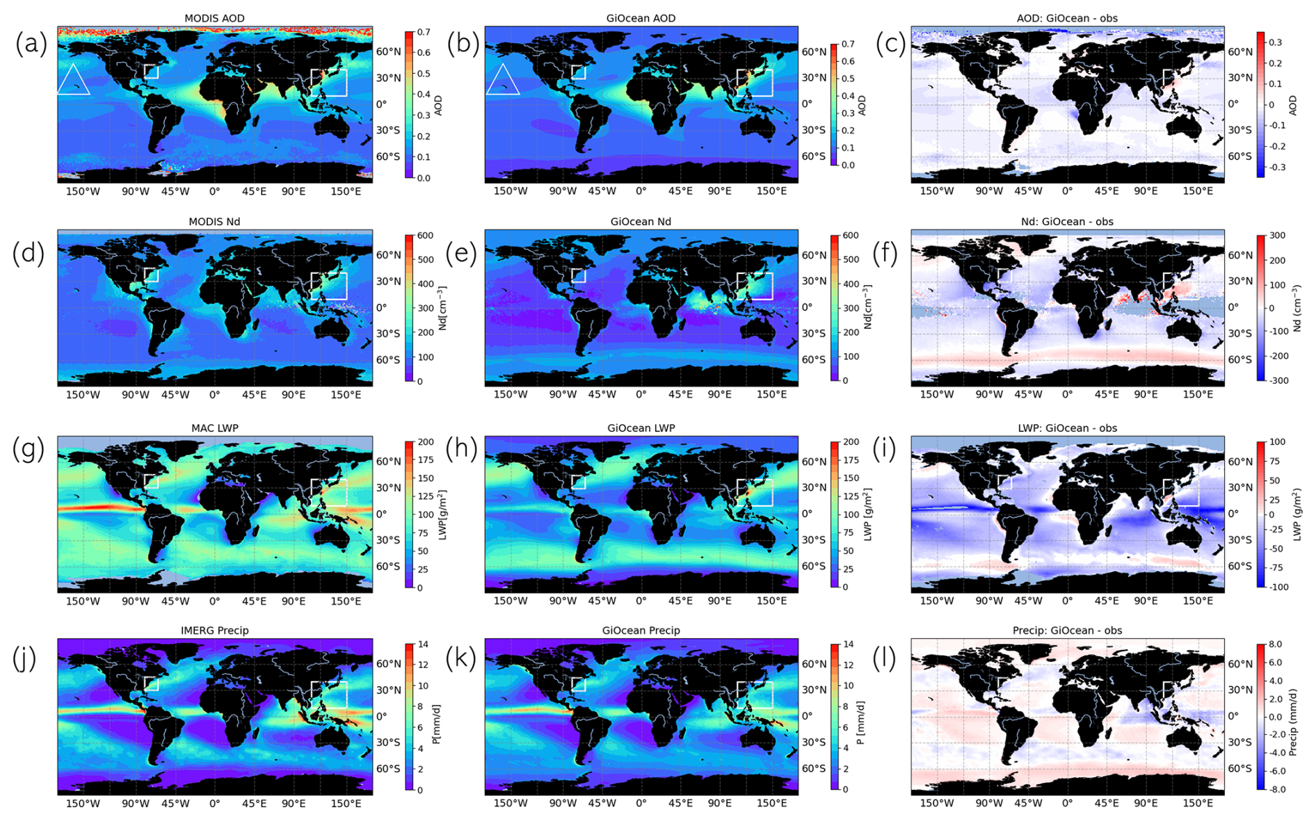
Figure 1 Comparison of the variables examined in this study between remote sensing observations (a, d, g, j) and GiOcean (b, e, h, k). The difference in variables betwen GiOcean and observations in shown in difference plot (c, f, i, l). GiOcean aerosol optical depth is compared to MODIS (a, b); GiOcean COSP Nd is compared to MODIS Nd from Grosvenor et al. (2018a) (d, e); GiOcean liquid water path is compared to MAC (g, h); and GiOcean precipitation is compared to IMERG (j, k). Study areas off the coast of the East Asia and North America are highlighted in white. The region of Kīlauea, where substantial effusive volcanic emissions occur, is indicated by triangles in (a) and (b).

To evaluate the temporal consistency between GiOcean and satellite observations, we calculate the Pearson correlation coefficient (r) between their respective regionally-averaged monthly time series. This analysis is performed for both the seasonal cycle and the decadal trend in two key outflow regions: East Asia and North America. High correlation values indicate that GiOcean effectively captures the temporal variability of key variables (e.g., AOD, Nd, LWP, precipitation rate) observed by satellites in that region.

Building on this regional focus, we characterize ACI using sensitivity metrics (Sect. 3.3) and a source–sink budget framework (Sect. 3.4). Under the source–sink budget framework, we include analysis over the NH ocean to provide a broader spatial context in terms of ACI beyond regional scales. Finally, we identify the dominant factors controlling the interannual variability of ACI in these regions (outflows of East Asia and North America, and NH ocean) using sensitivity tests based on random forest models.

3.1 Spatial variability

AOD from GiOcean and MODIS are in good agreement, except at very high latitudes (Fig. 1a, b and c). MODIS AOD retrievals in these regions are noticeably affected by a lack of clear-sky observations and surface contamination, especially in the Northern Hemisphere (Fig. 1a). This is attributed to MODIS often misinterpreting bright surface signals (i.e., snow surface) as aerosol scattering and reports spuriously high AOD (Levy et al., 2010). This discrepancy is clearly evident in the zonal-mean AOD (Fig. 2a) and the difference plot (Fig. 1c). Despite the inconsistency at high latitudes, AOD from GiOcean compares favorably to MODIS AOD with similar AOD in regions of heavy anthropogenic pollution, Saharan dust, and biomass burning (warmer colors in Fig. 1a, b). This is not entirely surprising since MODIS AOD is assimilated in GiOcean. In this way, observations of MODIS AOD are directly incorporated into the GiOcean reanalysis through data assimilation techniques, leading to high agreement between the two datasets, especially in regions where MODIS retrievals are reliable (e.g., ocean surfaces and clear-sky conditions). AOD is not a direct proxy for liquid-cloud relevant CCN, but the agreement in AOD between GiOcean and MODIS supports GiOcean having the right overall aerosol optical properties and hopefully a reasonable distribution of CCN following from that.

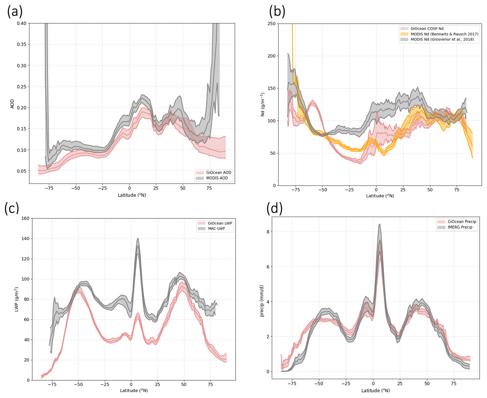
Figure 2 Comparison of zonal-mean oceanic quantities from GiOcean (pink) and satellite observations (gray). (a) Aerosol optical depth (AOD) from GiOcean (pink) and from MODIS (gray); (b) Cloud droplet number concentration (Nd) from GiOcean COSP output (pink) and MODIS, with values from Grosvenor et al. (2018a) shown in gray and from Bennartz and Rausch (2017) shown in orange; (c) Liquid water path (LWP) from native GiOcean output (pink) and MAC-LWP (gray); and (d) Precipitation rate from GiOcean (pink) and IMERG (gray). Shading represents the 95 % confidence interval of interannual variability.

Although the overall AOD pattern in GiOcean and MODIS are very similar (Fig. 2a), AOD in GiOcean is systematically lower over ocean compared to MODIS (Fig. 2a). A possible explanation for the small differences between GiOcean AOD and satellite AOD is the differences in AOD sampling between the GiOcean reanalysis and remote sensing observations. GiOcean AOD is assimilated from measurements collected by both the Terra and Aqua satellites (Buchard et al., 2016) (the Terra satellite crosses the equator in the morning, while Aqua crosses in the afternoon). Since AOD is influenced by the diurnal cycle (Balmes et al., 2021), these differences in overpass times can lead to discrepancies in the AOD observed by each satellite. Comparing satellite AOD sampled during Aqua satellite to GiOcean AOD can contribute to small differences (Fig. 2a). Additionally, several drivers may exacerbate the disagreement between the assimilated AOD in GiOcean and satellite retrievals. These include: (1) the influence of aerosol hygroscopic growth under high relative humidity conditions, which can enhance satellite-derived AOD but may not be fully captured in the model assimilation process (Twohy et al., 2009); (2) passive satellite sensors like MODIS retrieve AOD only under clear-sky conditions. However, GiOcean’s AOD may include scenes where real-world cloudiness would have prevented satellite retrievals, leading to a mismatch in AOD sampling between GiOcean and satellite-based observations; (3) limited representation of new particle formation events in GiOcean in the Southern Ocean boundary layer may lead to underestimation of aerosol concentrations and AOD (McCoy et al., 2021; Gordon et al., 2017); and (4) although GiOcean assimilates satellite AOD, the assimilation is constrained by retrieval uncertainties in this pristine and frequently cloudy region. As a result, model biases in aerosol processes and the inherently low aerosol concentrations may still contribute to differences between GiOcean and MODIS AOD, particularly over the Southern Ocean. Lower AOD in GiOcean is also apparent in the area downwind from Kīlauea (triangles on Fig. 1a, b), which are areas of substantial effusive volcanic emissions (McCoy et al., 2018a; Carn et al., 2017) (Fig. 1a, b). Although volcanic SO₂ emissions in GiOcean are constrained by observations from the OMI instrument aboard NASA's Aura satellite (Carn et al., 2015), the dataset provides only annual mean SO₂ emission rates. This temporal resolution is insufficient to capture short-term degassing events, leading to potential underrepresentation of short-term volcanic SO₂ contributions. For example, accurately representing eruptions such as those at Kīlauea in 2008 and 2018 requires daily-resolved emissions (Breen et al., 2021).

GiOcean COSP Nd generally aligns well with the MODIS retrieval. Both datasets show elevated Nd near heavily industrialized areas and in regions influenced by biomass burning (e.g., Namibia) and Saharan dust, consistent with enhanced AOD (Fig. 1a, b, c and d, e, f: warmer colors). GiOcean tends to report lower Nd over tropical and subtropical regions compared to MODIS (Figs. 1f, 2b). While the random uncertainty in individual MODIS Nd retrievals can be large (up to 78 %), this uncertainty decreases with averaging (Grosvenor et al., 2018b). However, systematic differences due to sampling and retrieval filtering remain and may contribute to the observed discrepancy (Gryspeerdt et al., 2022). As shown in Fig. 2b, GiOcean COSP Nd output falls between values reported by Bennartz and Rausch (2017) and Grosvenor et al. (2018b), both based on MODIS data. There is some indication that GiOcean may systematically underestimate Nd in pristine subtropical regions of the Southern Hemisphere (around 25° S), possibly due to GAAS underestimating sea salt concentrations (Randles et al., 2017). Conversely, GiOcean COSP Nd is higher than MODIS along remote southern storm tracks (around 50° S in Fig. 1f), potentially due to convective enhancement of Nd, parameterized in GiOcean but not in the MODIS algorithm. These differences may not be statistically significant, and improved Nd datasets are needed to better understand the contributing factors.

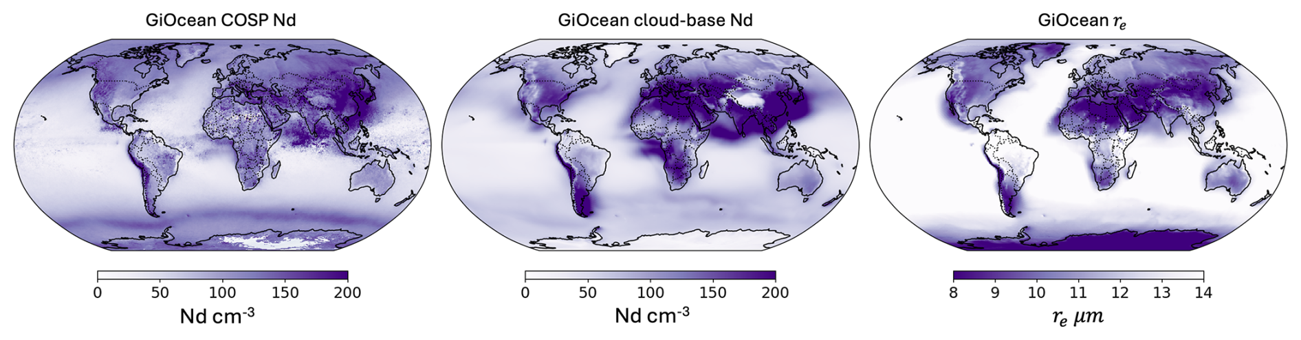
Figure 3 Annual mean cloud droplet number concentration (Nd) from GiOcean calculated from COSP output (left) and at cloud base (center), and cloud drop effective radius (r_e) (right). Global spatial correlation between annual mean r_e (right) and GiOcean COSP Nd (left) is −0.73, and between annual mean r_e (right) and GiOcean cloud-base Nd (left) is −0.75.

Figure 3, expands the analysis of Fig. 1 by including continental regions, comparing Nd values from the GiOcean COSP output (left panel) with those calculated at cloud base (center panel). While both datasets show broadly similar spatial patterns, the GiOcean COSP Nd tends to be slightly lower than Nd at cloud base in regions with heavy anthropogenic aerosol emissions. The greatest Nd appears in both datasets along the west coasts of North and South America, Europe, Southeast Asia, and South Africa. However, the GiOcean COSP value shows greater Nd at higher latitudes in both hemispheres compared to the cloud base values, a feature also evident in Fig. 1e. The origin of this discrepancy may stem from the retrieval algorithm used in GiOcean's COSP Nd, which tends to preferentially sample scenes with high liquid cloud fraction – conditions that become increasingly rare near the poles, while there is no such filtering to the cloud base Nd values.

Figure 3 also presents the cloud effective radius (r_e) from the GiOcean output. A strong inverse relationship between r_e and Nd is observed. The global spatial correlation between mean r_e and Nd is −0.73 for the GiOCean COSP product and −0.75 at cloud base, reflecting the microphysical basis of Twomey effect: higher cloud condensation nuclei (CCN) concentrations lead to a greater number of smaller droplets, enhancing cloud reflectivity (Twomey, 1991). This confirms GiOcean's capacity to capture such microphysical processes. It is important to note that r_e is also a parameter in the retrieval algorithm used for the GiOcean COSP output. The observed decrease in r_e at high latitudes could therefore inflate Nd values in these regions. Although the microphysical basis of Twomey effect is prominent globally, it is not ubiquitous. For example, in Southeast Asia, high Nd does not correspond to small r_e. Likewise, R_eff decreases at higher latitudes, particularly in the Northern Hemisphere, without a corresponding increase in cloud base Nd-likely due to reduced water availability in colder conditions. These features may reflect aerosol-induced adjustments to liquid water path (LWP) and precipitation, which are explored further in Sect. 3.3.

LWP is systematically lower in GiOcean than observed by microwave radiometers as aggregated and harmonized in the MAC-LWP data set (Figs. 1g, h, i and 2c: pink and gray), particularly true in the Tropical regions (30° S to 30° N). However, some of this discrepancy may be attributable to potential systematic errors in microwave LWP as discussed in Sect. 2.3.2. Within the extratropics we estimate this error to be ±10 % (Song et al., 2024; Elsaesser et al., 2017), which may bring the observations closer or further, but cannot entirely explain this observation-reanalysis discrepancy (Fig. 2c). The discrepancy is larger in relatively high precipitation regions in the tropics. Overall this points to an unrealistically low LWP in GiOcean, despite observational uncertainty.

GiOcean and IMERG exhibit consistent zonal patterns in precipitation rate across latitudes, with both capturing the major meridional features (Fig. 2d). This consistence may stem from GiOcean's assimilation of SST, which controls large-scale circulation features such as the Intertropical Convergence Zone (ITCZ) and midlatitude storm tracks. However, slight differences in magnitude are evident across latitudes. GiOcean overestimates precipitation in regions with low precipitation rates (e.g., subtropics and regions poleward of 60°) and exhibits a sharper transition to very low precipitation in the subtropical dry zones near the western sides of continents (Fig. 1j, k). This may be partially attributable to biases in GiOcean, but may also relate to IMERG struggling to detect the prevalent drizzle in these regions (Pradhan and Markonis, 2023).

3.2 Temporal variability

3.2.1 Seasonal cycle

Having characterized the spatial patterns of aerosols, cloud properties, and precipitation, we now examine their temporal variability. Our analysis focuses on the North American and East Asian outflow regions, as indicated by the rectangular boxes in Fig. 1, because these regions are major sources of anthropogenic aerosol emissions and are known to strongly influence downwind cloud properties (McCoy et al., 2018a). These two regions also show contrasting sensitivity of r_e to Nd (Fig. 3). We examine the seasonal and decadal variability in each region.

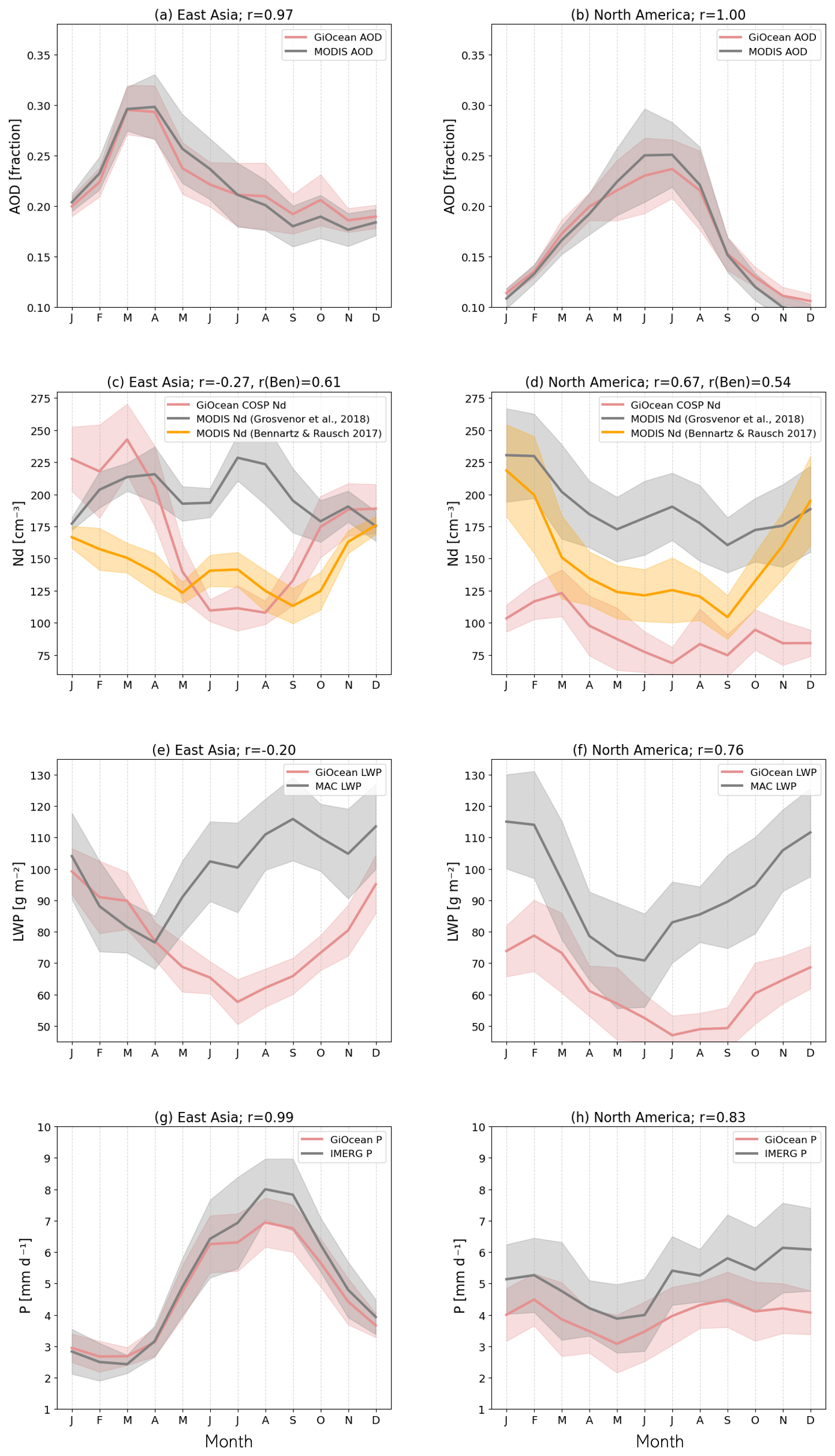
Figure 4 Comparison of seasonal cycles in the outflow regions of East Asia (a, c, e, g) and North America (b, d, f, h) from GiOcean (pink) and satellite observations (gray). AOD (a, b), Nd (c, d), LWP (e, f), and precipitation rate (g, h). The GiOcean outputs and the sources of satellite observations used for comparison are consistent with the description in Fig. 2. Solid lines show 12-month climatological mean seasonal cycles, and the shading shows ± standard deviation across all years (2003–2015) for each month. The correlation (r) between the monthly climatology time series of GiOcean and satellite observations is shown in the panel title. r(Ben) is the correlation between Bennartz Nd (Bennartz and Rausch, 2017) and GiOcean COSP Nd.

Seasonal variability in AOD shows strong agreement between GiOcean and MODIS, with correlation coefficients (r) near 1 in both the East Asian and North American outflow regions (Fig. 4a, b). Peak AOD occurs during boreal spring in the East Asian outflow and during boreal summer in the North American outflow. This is expected as AOD is assimilated in GiOcean.

In the East Asian outflow, Nd from GiOcean exhibits a pronounced seasonal cycle with a peak during winter and a minimum in summer (Fig. 4c: pink). This pattern is likely driven by increased precipitation between June and September, peaking around August, possibly enhanced by the summer monsoon as indicated by the precipitation seasonal cycle (Fig. 4g: pink). Enhanced wet scavenging during this period reduces both aerosol concentrations and droplet number (Fig. 4a, c: pink). However, this effect may be confounded by increased biomass burning emissions during the same period (Kim et al., 2007). Interestingly, this strong seasonal signal in Nd is not evident in the MODIS retrieval over the East Asian outflow region (Fig. 4c: gray and orange), although notable discrepancies exist among different Nd datasets, with the data from Bennartz and Rausch (2017) showing a somewhat stronger seasonal cycle than the data from Grosvenor et al. (2018a), though still weaker than in GiOcean.

In contrast, the North American outflow region displays a weaker seasonal cycle in Nd in GiOcean, with lower values during summer, and better consistency between GiOcean COSP Nd and the observational datasets, yet with significant differences in absolute value (Fig. 4d). The consistency in seasonal trends across datasets suggests that GiOcean and satellite observations capture similar seasonal signals. However, differences in absolute Nd values may partly reflect the spread across satellite retrieval algorithms, referred to as the retrieval bundle, which represents a form of systematic observational uncertainty (Elsaesser et al., 2025).

Overall, we found larger discrepancies in the seasonal cycle of Nd over the East Asian outflow region (Fig. 4c) compared to the North American outflow, which may be due to active convection, which complicates the retrieval and modeling of Nd. Reanalysis products often exhibit greater biases in simulating Asian meteorology, and the assumptions underlying MODIS retrievals may break down under these meteorological conditions. As a result the disagreement in Nd seasonal cycle is higher over East Asian outflow than over the North American outflow.

The seasonal cycles of GiOcean and MAC-LWP both exhibit peak LWP in winter in the East Asian and North American outflow regions (Fig. 4e, f), but substantial differences in the overall seasonal patterns and magnitude remain. The GiOcean and MAC-LWP show a better agreement during winter in the East Asian outflow region, which might be due to the relatively accurate MAC-LWP estimates during winter over the study regions (Elsaesser et al., 2017). However, correlation between MAC-LWP and GiOcean is weakly negative in East Asian outflow region (Fig. 4e). In the North American outflow region, the seasonal variability of LWP is mostly captured by GiOcean, with a correlation of r=0.76 compared to satellite observations (MAC-LWP) (Fig. 4f).

Seasonal variability in precipitation rate in GiOcean matches IMERG in both the East Asian and North American outflow regions, with differences statistically indistinguishable at the 95 % confidence level across all months (Fig. 4g, h). There is a high correlation of r=0.99 between GiOcean and IMERG in the East Asian outflow, where a strong seasonal cycle exists (Fig. 4g). In the North American outflow where the seasonal cycle is weaker the agreement is also good, with a correlation of r=0.83 (Fig. 4h). Although GiOcean slightly underestimates the amplitude of seasonal variation, it reproduces the broad features of the cycle, including a minimum in late spring and a gradual increase in precipitation from summer into fall. The high correlation between GiOcean and observed precipitation rates in the East Asia outflow (Fig. 4g) is consistent with the fact that GiOcean is constrained by SST fields from the GEOS-IT reanalysis. SST strongly influences moisture convergence through its impact on large-scale atmospheric circulation, and therefore plays a key role in shaping seasonal precipitation patterns (Seager et al., 2010).

3.2.2 Interannual variability

The decadal trend in aerosol and cloud properties is a useful proxy for understanding the radiative forcing from ACI (Wall et al., 2022; McCoy et al., 2018a; Bennartz et al., 2011). The monthly time series of AOD, Nd, LWP and precipitation rate are shown in Fig. 5.

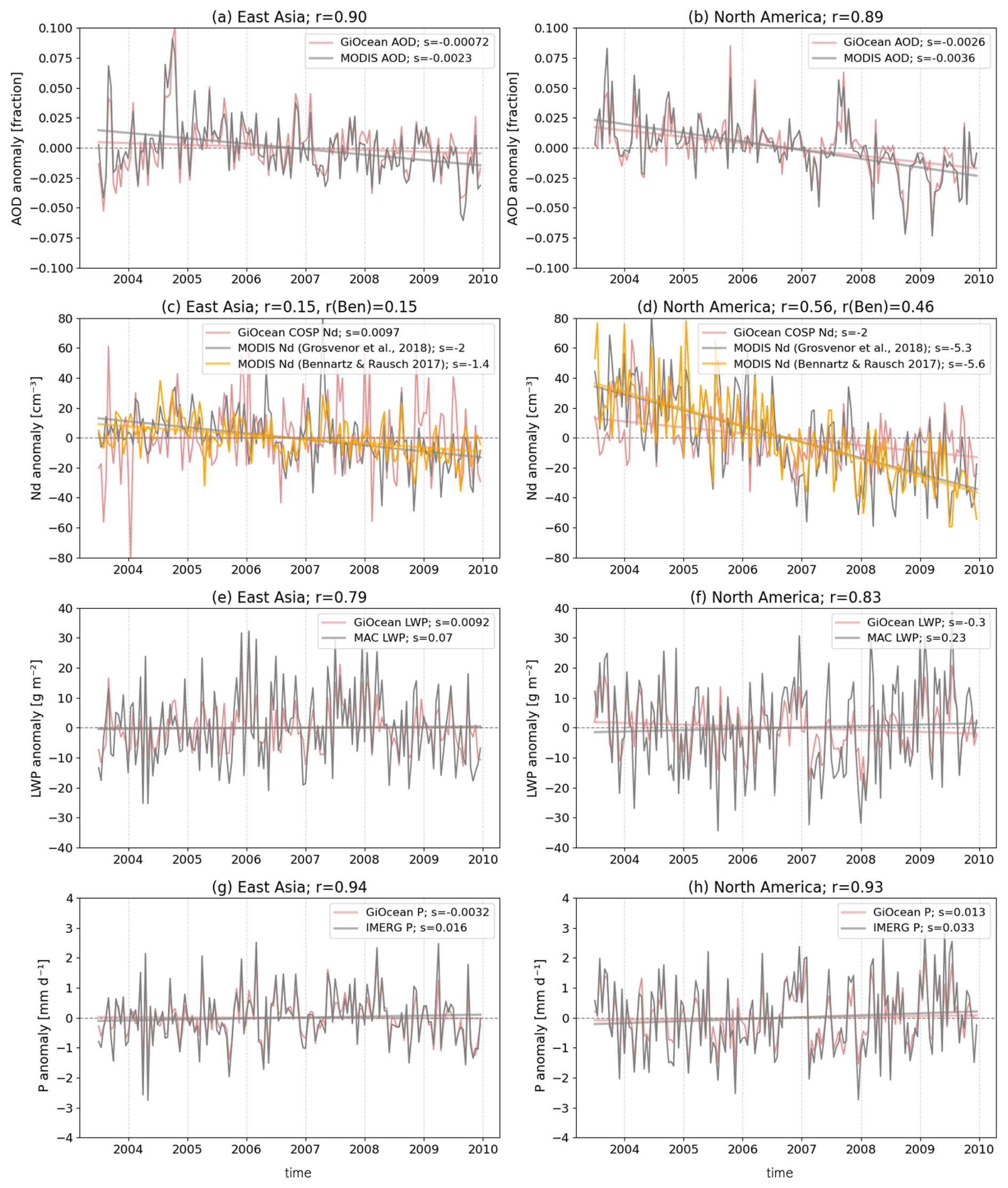
Figure 5 The monthly anomaly time series in the outflow regions of East Asia (a, c, e, g) and North America (b, d, f, h) from GiOcean (pink) and satellite observations (gray or orange). AOD (a, b), Nd (c, d), LWP (e, f), and precipitation rate (g, h). The GiOcean outputs and the sources of satellite observations are consistent with the description in Fig. 2. Monthly anomalies are calculated by removing the long-term monthly climatology from the original time series. The correlation (r) between the monthly anomaly time series of GiOcean and satellite observations is shown in the panel title. r(Ben) is the correlation between Bennartz Nd (Bennartz and Rausch, 2017) and GiOcean COSP Nd. Linear trend lines are shown for each dataset in the line labels, with the slope (s) indicating the trend per month. Units of slope: (a, b) in month⁻¹; (c, d) in cm⁻³ month⁻¹; (e, f) in g m⁻² month⁻¹; and (g, h) in mm d⁻¹ month⁻¹.

Both GiOcean and satellite observations show an overall downward trend in AOD, along with good agreement in the monthly anomaly time series across the two focus regions (Fig. 5a, b). This is consistent with trends in sulfur dioxide emissions in these regions driven by emissions control measures in the East Asian and North American outflow regions (McCoy et al., 2018a).

Generally MODIS and GiOcean broadly agree with the trend in Nd with a downward trend through the observational period in the North American outflow (Fig. 5d), suggesting that the observed decadal trend in Nd may be related to aerosol affecting cloud microphysical properties in that region. The downward trend in Nd in the North American outflow is also consistent with previous evaluation of trends in Nd (McCoy et al., 2018a). During the period with concurrent observational data over the East Asian outflow, MODIS Nd from Bennartz and Rausch (2017) and Grosvenor et al. (2018b) shows a downward trend while GiOcean COSP Nd is relatively flat (Fig. 5c). This may result from the disproportionate influence of convection over the region which tends to introduce uncertainty in both the retrieval and the reanalysis.

The monthly anomaly time series in LWP are consistent between MAC-LWP and GiOcean in the East Asian and North American outflows, with correlation coefficients close to 0.8 in both regions and no clear overall upward or downward trends during the study period (Fig. 5e, f). GiOcean has the microphysics scheme necessary to produce precipitation suppression and this may lead to the covariation of LWP and Nd from 2003 to 2015 in the East Asian outflow region, where increases in Nd are consistently accompanied by increases in LWP in GiOcean, and vice versa (Fig. 5c,e: pink, Fig. S1 in the Supplement). It must also be noticed that the response of LWP is not entirely driven by cloud microphysical processes in GiOcean. Large-scale moisture convergence, which is influenced by SST and large-scale atmospheric circulation (Zelinka et al., 2018), also plays a key role. The base model of GiOcean is constrained by SST and a moisture analysis increment is applied every six hours to correct the state of the model. The consistency in the monthly time series between observed LWP and GiOcean LWP suggests that GiOcean has the ability to represent both the moisture supply and the cloud response to Nd that are necessary to reproduce LWP interannual variability.

In keeping with the seasonal cycle, the monthly precipitation anomaly time series from GiOcean and IMERG are in good agreement and exhibit concurrent variation with LWP anomalies in GiOcean and observations across both regions during the study period. While consistent, there isn't a particularly strong overall trend in precipitation in either study region (Fig. 5g, h). Given the overall magnitude of the precipitation rate in these regions (Fig. 1h), this points to a fairly large interannual variability in the precipitation flux demand by the atmosphere that makes it difficult to disentangle the role of meteorology, data assimilation, aerosol, and precipitation-related scavenging in driving changes in cloud properties (i.e. Nd and LWP) (Wood et al., 2012; Kang et al., 2022). In the following section we attempt to evaluate the representation of ACI in GiOcean against satellite observations.

3.3 Aerosol-cloud interactions in GiOcean and observations

While the primary focus of this study is on jointly analyzing the effect of sources and sinks on cloud properties, we include this sensitivity analysis of Nd versus AOD and LWP versus Nd to facilitate comparison with previous studies that have emphasized these pairwise relationships.

3.3.1 Inferred sensitivity of cloud droplet number concentration to AOD

AOD is commonly used in satellite-based studies and model evaluations of how aerosols alter cloud microphysical properties, despite its known limitations as a proxy for cloud condensation nuclei (CCN) (Liu et al., 2024; Quaas et al., 2010).

We found a positive inferred sensitivity of Nd to AOD in the East Asian outflow region in both the GiOcean reanalysis and satellite observations (Fig. 6: circles), indicating that increases in AOD are associated with increases in Nd. This is consistent with the aerosol indirect effect where increased aerosol enhances cloud droplet activation (Twomey, 1977). The stronger inferred sensitivity in GiOcean (S=0.96: pink circles in Fig. 6a) compared to observations (S=0.64: gray circles) suggests that cloud droplet formation in the model responds more strongly to changes in AOD in GiOcean over East Asian outflow. However, this stronger slope does not imply that GiOcean has a stronger aerosol–cloud microphysical response at a given AOD. In fact, despite the higher inferred sensitivity, the absolute Nd in GiOcean is lower than in MODIS for the same AOD (Fig. 6a). This may suggest that GiOcean overestimates the relative response of Nd to aerosol changes, but underestimates the overall efficiency of aerosol activation into cloud droplets.

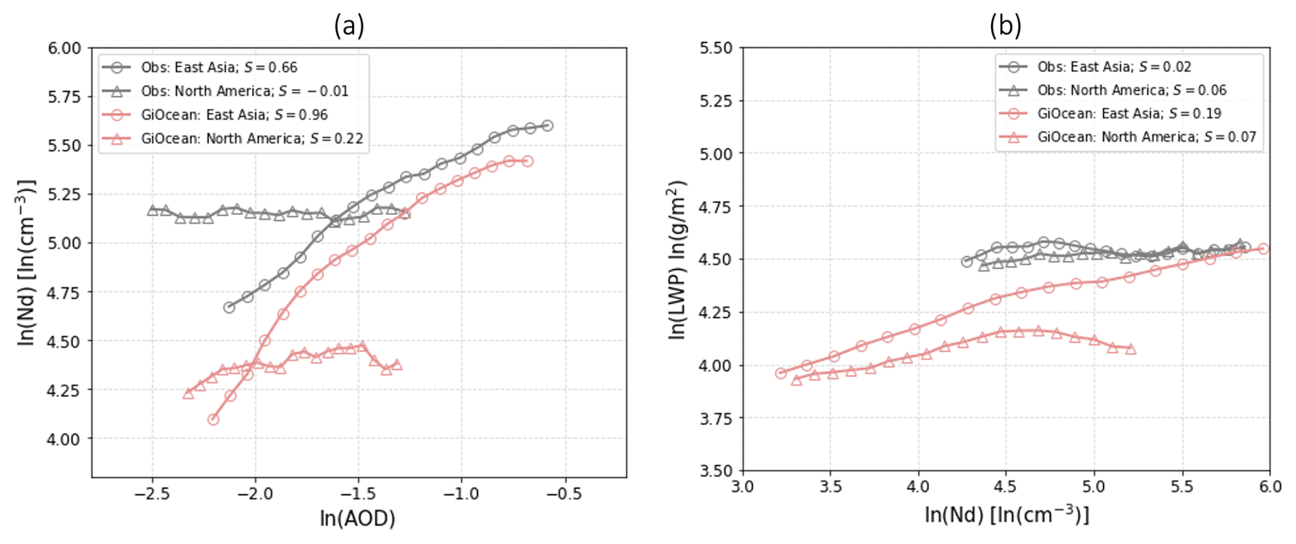
Figure 6 (a) Inferred sensitivity (S) of cloud droplet number concentration (Nd) to aerosol optical depth (AOD), and (b) inferred sensitivity of liquid water path (LWP) to Nd, based on both GiOcean (pink) and satellite observations (gray) in the outflow regions of East Asia (circles) and North America (triangles), using the sensitivity metrics defined in Eqs. (1) and (2).

Similarly, we examined the inferred sensitivity of Nd to AOD in the North American outflow region (Fig. 6: triangles). The inferred sensitivity is slightly positive (S=0.22: pink triangles in Fig. 6) in GiOcean, while near zero in observations (gray triangles in Fig. 6). The low sensitivity of Nd to AOD over the North American outflow is primarily due to sampling. In GiOcean, COSP-derived Nd is sampled following the cloud-filtering criteria of Grosvenor et al. (2018a) to match the sampling of MODIS Nd. When cloud base Nd is used, or when COSP-derived Nd is recalculated without filtering, a strong positive sensitivity of Nd to AOD becomes apparent (Fig. S2). This indicates that the low sensitivity of Nd to AOD is inherent to the Nd sampling strategy over the North American outflow, rather than a result of GiOcean being unable to represent aerosol–cloud microphysical responses. We also note that the analysis of the inferred sensitivity of Nd to AOD does not account for the role of meteorological factors in driving the sensitivity terms. Precipitation scavenges aerosol and cloud droplets, potentially dampening the signal of changes in cloud properties induced by aerosol perturbation. We will discuss the role of precipitation in the Sect. 3.4.1.

3.3.2 Inferred sensitivity of liquid water path (LWP) to Nd

In addition to changes in cloud microphysics, changes in Nd can also change macrophysical cloud properties. The inferred sensitivity of LWP to Nd is characterized using Eq. (2). In observation, there is a very low inferred sensitivity of LWP to Nd in both regions (S = 0.02–0.06) (Fig. 6b: gray shapes). Instead, GiOcean shows stronger response in LWP with Nd than observed in both regions (Fig. 6b: pink). In East Aisan outflow, GiOcean shows monotonic increase in LWP with Nd (Fig. 6b: pink circles). In the North American outflow region LWP first increases with Nd in the low Nd regime and and then decrease with Nd in the high Nd regime (Fig. 6: pink triangles). This is consistent with the theoretical evidence of competing precipitation suppression and entrainment effects on liquid cloud adjustment (Ackerman et al., 2004). However, interpreting the relationship between Nd and LWP is complicated by coalescence-scavenging from precipitation (Mikkelsen et al., 2025). Precipitation is a strong sink of Nd in marine low clouds (Kang et al., 2022; Wood et al., 2012), and depletes aerosol at cloud base (Textor et al., 2006). The amount of liquid water in clouds (i.e., LWP) also depends on how much rain the clouds produce, which is strongly controlled by environmental factors such as large-scale atmospheric circulation and sea surface temperature patterns.

To illustrate the importance of precipitation in the context of aerosol affecting cloud microphysical properties (Eq. 1) and liquid cloud adjustment induced by changes in Nd (Eq. 2), we interpret the budget of Nd and LWP using a sink-source perspective in Sect. 3.4.

3.4 Source-sink budgets of cloud microphysics and macrophysics

As outlined above, GiOcean generally replicates spatial and temporal patterns of AOD and precipitation rate (Figs. 1, 4, and 5). However, the correspondence between GiOcean and observations regarding cloud microphysics and macrophysics (i.e. Nd and LWP) is less robust. To understand the sources of these biases, it is important to determine whether they arise from how GiOcean simulates the response of liquid clouds to aerosols (sources), or from how it represents the influence of moisture demands from the large-scale environment (sinks via precipitation-scavenging). This requires separating the effects of these two factors on the cloud properties. Here, we consider cloud droplet number (Nd) and cloud liquid mass (LWP) in terms a simple source-sink budget framework to evaluate monthly patterns of both quantities in the outflow regions identified in Fig. 1. We also examine a broader spatial scale covering the Northern Hemisphere (15–65°), where most anthropogenic emissions originate.

3.4.1 Source-sink budget of Nd

To visualize the response of Nd to AOD or precipitation rate we formulated the source-sink budget of Nd as two-dimensional lookup tables using monthly datasets at each grid point over the study regions. The lookup table is constructed by dividing monthly AOD and precipitation rate into 50 × 50 two-dimensional bins and bin averages are calculated within each bin. This allows us to examine how Nd responds across varying combinations of AOD and precipitation. We note that because the lookup tables are constructed using monthly data across all grid points, the Nd–AOD–precipitation relationships reflect a combination of spatial and temporal variability. Due to the large range and log-normal distributions of precipitation rate and AOD we use logarithmic bins. The dependence of Nd on AOD and precipitation rate for each outflow region and for GiOcean and observations is visualized in the lookup tables in Fig. 7.

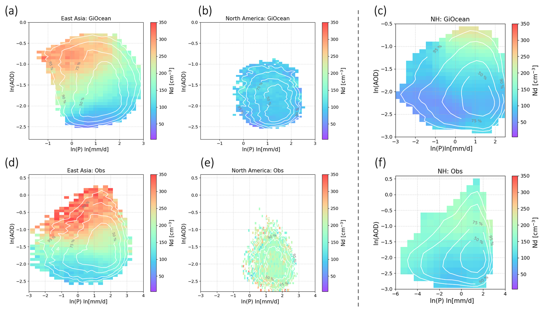
Figure 7 Cloud droplet number (Nd) composited on AOD and precipitation rate in GiOcean (abc) and from observations (def) and in the regions off the coast of East Asia (ad), North America (be) and Northern hemisphere ocean (cf). The density of points is indicated by white contours. The percentage labeled on each contour represents the fraction of monthly data points contained within that contour. The outermost white contour encloses the 2-D density region containing 95 % of the monthly data points, effectively excluding extreme outliers.

By analyzing the marginal distribution of Nd across AOD while holding precipitation rate fixed, we assess how aerosol alters cloud properties. Conversely, examining Nd across precipitation rate while holding AOD fixed provides insight into how precipitation controlled by large-scale environment modulates Nd through wet scavenging.

Overall, the ranges of precipitation rate and AOD in GiOcean match those from satellite observations in the outflow regions of both East Asia and North America, as well as over the broader Northern Hemisphere (Fig. 7). In East Asia, the range of precipitation rate and AOD spans nearly two orders of magnitude in both GiOcean and observations (Fig. 7a, d), whereas in North America, it covers only one.

In the North American outflow, the pattern of Nd as a function of AOD and precipitation rate is not clear for either GiOcean or observations (Fig. 7b, e). This might be because the sampling of Nd following Grosvenor et al. (2018a), which can obscure the sensitivity of Nd to AOD and precipitation in this region. In contrast, a clearer relationship emerges in the outflow region of East Asia and over the Northern Hemisphere ocean (first and third columns of Fig. 7).

In the East Asian outflow region (first column of Fig. 7), GiOcean Nd increases with AOD at fixed precipitation rates (Fig. 7a), indicating a microphysical response of Nd to aerosol loading at fixed coalescence-scavenging. Similarly, when AOD is held approximately constant within its range, Nd decreases with increasing precipitation (high Nd is associated with low precipitation rate). This pattern suggests that the Nd budget in GiOcean reflects a combination of a source driven by effective CCN and a sink associated with wet scavenging (via precipitation), which is modulated by environmental conditions. We use the same methodology to analyze the Nd pattern in satellite observations (Fig. 7c). Similar to GiOcean, satellite data shows an increase in Nd with increasing AOD at fixed precipitation rates, indicating a consistent aerosol–cloud microphysical relationship. However, unlike GiOcean, we find a much weaker covariance between precipitation rate and Nd when AOD is held constant, particularly at low AOD concentrations. This might suggest that, in the observational data, the precipitation sink of Nd via wet scavenging is either less pronounced or obscured by retrieval uncertainties or other confounding factors such as satellite sampling biases, differences in vertical overlap between precipitation and aerosol layers, or cloud regime heterogeneity (Grosvenor et al., 2018b). The more pronounced link between Nd and precipitation rate in GiOcean might also indicate that the precipitation dependence of Nd may be amplified by the representation of coalescence scavenging in GiOcean.

Extending the compositing analysis using lookup tables to the NH ocean (third column of Fig. 7), the relationship between Nd and precipitation rate becomes weaker. This weakened link is consistent in both GiOcean and satellite data (Fig. 7c, f).

Overall, the dependence of Nd on AOD and precipitation rate inferred from the compositing in Fig. 7 is consistent with prior expectations based on Wood et al. (2012). Increasing AOD corresponds to an increase in CCN-relevant aerosol and an increasing in Nd. This behavior is consistently captured in both GiOcean and satellite observations across regional and broader Northern Hemisphere analyses (Fig. 7a, d, c, f). Increasing precipitation removes cloud droplets through coalescence scavenging, leading to a decrease in Nd with increasing precipitation rate. This pattern is more clearly represented in GiOcean over heavily polluted regions such as East Asian outflow (Fig. 7a), but is less pronounced in satellite observations over the same area (Fig. 7d). The weak link between precipitation and Nd is also seen in both GiOcean and satellite data over the broader NH ocean (Fig. 7c, f). Taken together, this suggests that precipitation scavenging of Nd may be overestimated in heavily polluted regions in GiOcean.

3.4.2 Source-sink budget of LWP

The interpretation of the LWP lookup tables follows the same logic as that of the compositing analysis using Nd lookup tables discussed earlier in Sect. 3.4.1. We assess how liquid clouds adjust to changes in Nd by analyzing variations in LWP across Nd bins while holding precipitation rate constant. Conversely, we evaluate how large-scale moisture convergence influences liquid cloud amount (i.e., LWP) by examining LWP across precipitation bins while holding Nd constant (Fig. 8). Furthermore, by comparing the relative sensitivity of LWP to changes in Nd and precipitation, we can assess how liquid cloud adjustment responds to aerosol and environmental controls in both GiOcean (Fig. 8a, b) and satellite observations (Fig. 8c, d).

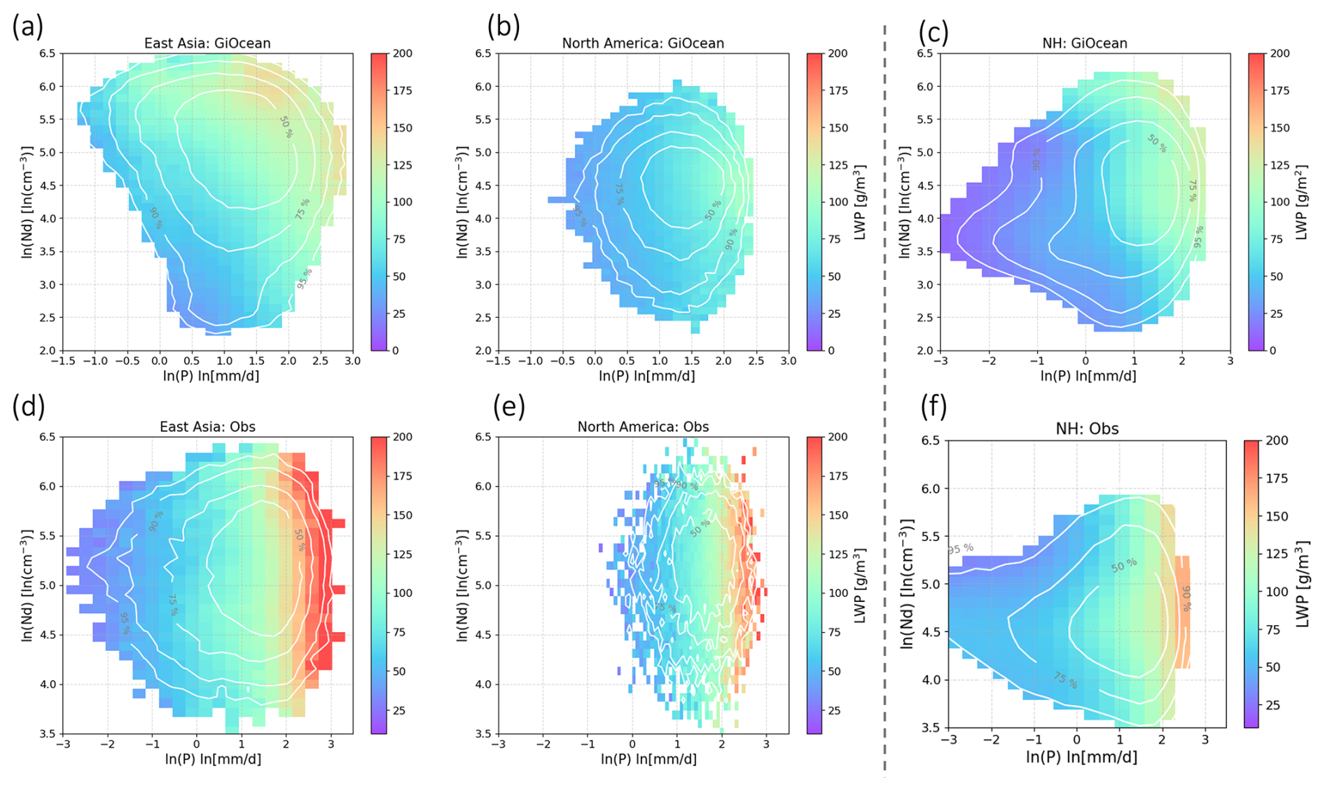
Figure 8 Similar to Fig. 7 but showing liquid water path composited on Nd and precipitation rate in GiOcean (abc) and from observations (def) and in the regions off the coast of East Asia (ad), North America (be), and over Northern Hemisphere ocean (cf).

The dependence of LWP on Nd and precipitation rate is consistent with a priori expectations. In all study regions, and in both observations and GiOcean, LWP increases with precipitation rate when Nd is held constant (Fig. 8), consistent with the interpretation that greater large-scale moisture convergence leads to increased cloud water content, assuming precipitation efficiency remains approximately unchanged (via fixed Nd). This suggests that higher precipitation rates reflect not only enhanced removal of cloud water, but also stronger moisture supply to the cloud layer.

The patterns of inferred liquid cloud adjustment shows varying degree of agreement between GiOcean and satellite observations over different study regimes (Fig. 8). In the North American outflow region, both GiOcean (Fig. 8b) and satellite observations (Fig. 8e) indicate a weak liquid cloud adjustment to Nd (weak variation in LWP with Nd at fixed precipitation rate). This consistency suggests that GiOcean realistically captures the weak liquid cloud adjustment in this region.

In the East Asian outflow, GiOcean reanalysis shows that LWP increases with higher Nd when precipitation rate is held constant (Fig. 8a). This pattern is consistent with the suppression of precipitation: at higher Nd, more LWP is needed to maintain the same precipitation rate due to reduced collision–coalescence efficiency. However, the liquid cloud adjustment through precipitation suppression is less pronounced in satellite observations over the East Asian outflow region (Fig. 8d). This may reflect limitations in satellite retrievals, such as uncertainties in Nd under multilayer cloud conditions or partial cloud cover (Zhang et al., 2016b; Grosvenor et al., 2018b), and uncertainty in LWP under heavy-precipitating regions (Elsaesser et al., 2017). Additionally, satellite observations represent instantaneous snapshots, which may not fully capture the temporal evolution of cloud water accumulation in response to aerosol loading. This may also indicate that the effects of precipitation suppression may be overestimated in GiOcean compared with what occurs in reality in the East Asian outflow region.

The NH ocean pattern is similar with that in the outflow of East Asia in GiOcean: LWP increases with Nd at fixed precipitation rate, indicating suppressed precipitation and accumulation of liquid water. This positive Nd–LWP relationship is especially pronounced at high precipitation rates (Fig. 8c). In contrast, satellite observations show a negative Nd–LWP relationship when precipitation rate is fixed, particularly at low precipitation rates. This negative Nd–LWP correlation is found across satellite retrieval methods (Gryspeerdt et al., 2019). This suggests that the contrast with GiOcean likely reflects model biases in representing cloud microphysics, rather than retrieval artifacts alone.

3.5 Analysis of the factors controlling Nd and LWP decadal variability

The compositing analysis using lookup tables built from monthly data at each grid points in Sect. 3.4 provides a diagnostic of the dependence of Nd and LWP on their sources and sinks, capturing a mixture of temporal and spatial variability. In this section, we characterize the factors driving historical trends in Nd and LWP, which is critical for quantifying the magnitude and evolution of radiative forcing from ACI (Wall et al., 2022), particularly in regions undergoing rapid changes in aerosol emissions, such as East Asia and North America (Bennartz et al., 2011).

To evaluate how the dependencies of Nd and LWP on their respective sources and sinks influence long-term temporal variations in cloud properties, we use Random Forest (RF) models trained on regionally-averaged monthly time series from three study domains: the outflow regions of East Asia, North America, and the NH ocean. Separate RF models of Nd and LWP are trained for GiOcean and satellite observations using source and sink variables as predictors (i.e., AOD and precipitation rate for Nd, and Nd and precipitation rate for LWP). We then conduct sensitivity experiments to assess how interannual variability in Nd and LWP responds to changes in their source and sink terms in GiOcean and satellite observations. The details of each RF experiment are as follows:

1. Full-predictor case: The Nd decadal trend is predicted based on the RF model using the original monthly time series of AOD (source) and precipitation rate (sink) at their regional means as predictors. Similarly, the LWP decadal trend is predicted based on RF model using the original time series of Nd (source) and precipitation rate (sink) as predictors. This full-predictor approach is applied to both satellite observations and GiOcean data. Predictions from this case are shown as gray solid lines in Figs. 9 and 10.

2. Fixed-sink case: In this scenario, we aim to predict the decadal trends of Nd and LWP based on RF models while holding the precipitation rate (sink) constant at its multiyear mean value. The source terms – AOD for Nd and Nd for LWP – are taken from the original monthly time series (GiOcean or satellite observations). RF model predictions from this case are shown as green solid lines in Figs. 9 and 10.

3. Fixed-source case: The decadal trends of Nd and LWP in GiOcean and satellite observations are predicted using the RF models by setting the source terms – AOD for Nd and Nd for LWP as constant at their multiyear mean values. The sink term (precipitation rate) varies over time based on values from GiOcean or satellite observations. The Nd and LWP decadal trends predicted by fixed-source are shown in pink solid lines in Figs. 9 and 10.

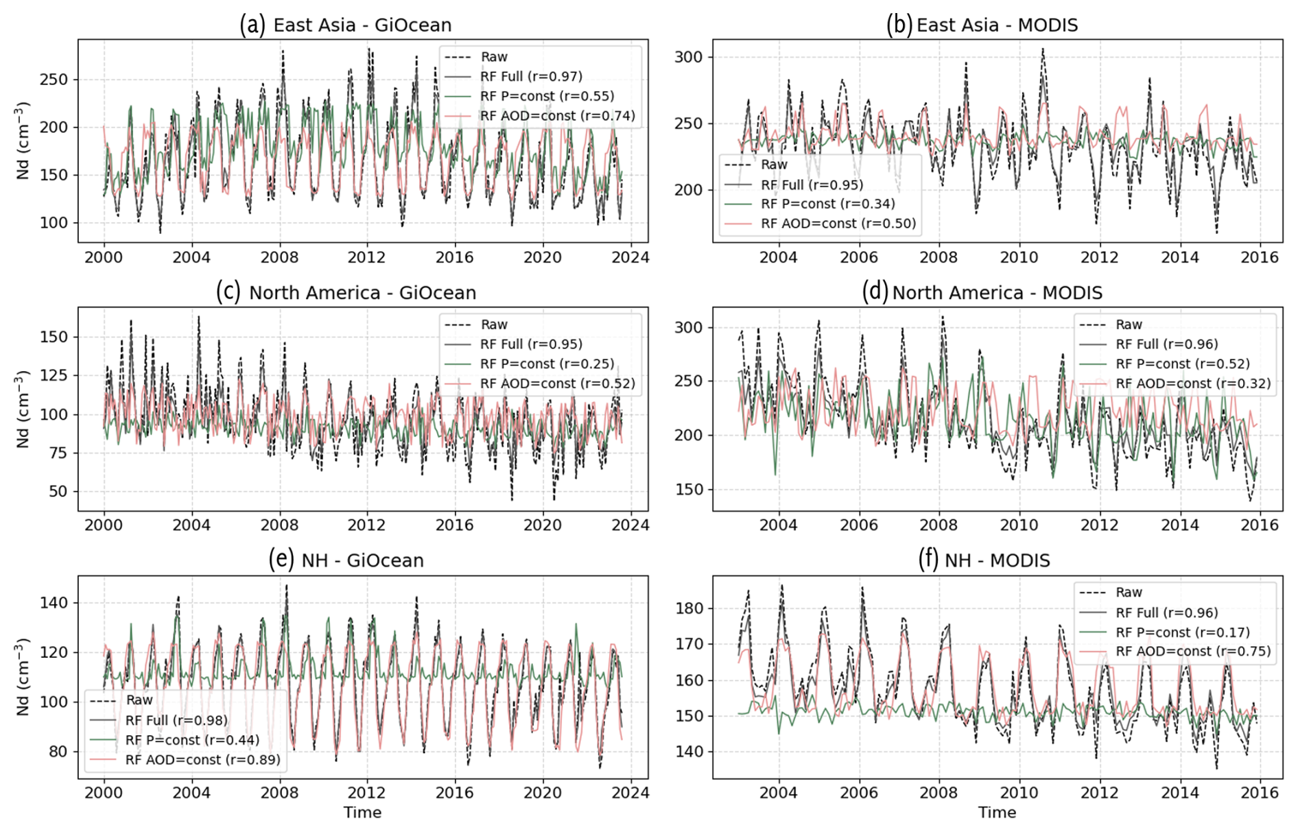
Figure 9 The monthly time series of Nd in the regions off the coast of (a, b) East Asia, (c, d) North America, and over (e, f) Northern Hemisphere ocean. The black dashed line represents the original Nd time series from GiOcean or MODIS, while the solid lines show predictions from Random Forest (RF) models. Three correlation diagnostics are included in the legend: RF Full (gray): Nd predicted by the RF model using all input variables from original datasets (sink + source), with the correlation (r) indicating how well the RF model captures year-to-year variability in regional-mean Nd. RF P = const (green): Prediction with precipitation rate (sink) held constant at its multiyear mean, used to assess the influence of sink on Nd interannual variability. The correlation coefficient (r) is calculated between the monthly time series of predicted Nd from the fixed-sink experiments and the original dataset. RF AOD = const (pink): Prediction with AOD (source) held constant at its multiyear mean, used to evaluate the influence of aerosol loading on Nd variability. Higher correlations indicate a stronger ability of the model to reproduce observed decadal variability of Nd under each condition.

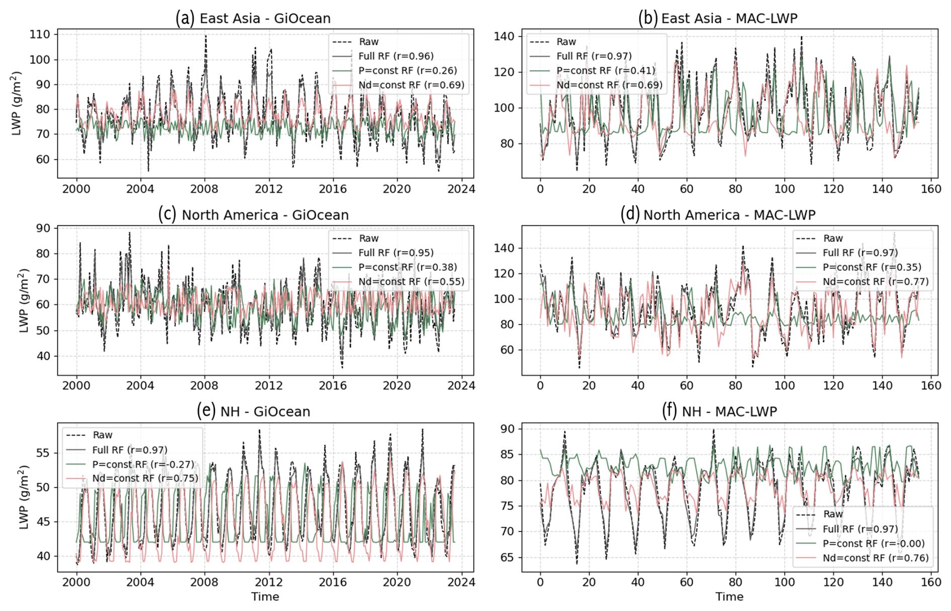
Figure 10 Same as Fig. 9, but showing the monthly time series of LWP for regions off the coasts of (a, b) East Asia, (c, d) North America, and (e, f) the Northern Hemisphere ocean. In this case, fixed-source experiments refer to holding Nd constant at its multiyear mean while allowing precipitation rate to vary monthly. Fixed-sink experiments refer to holding precipitation rate constant at its multiyear mean while allowing Nd to vary monthly.

We compare the fixed-source and fixed-sink predictions from RF models to the original (directly available from GiOcean and satellite observations) monthly time series of Nd and LWP. Specifically, we assess how well each sensitivity case captures the interannual variability by calculating the temporal correlation (r) between their predicted regional averaged monthly time series and that of the original datasets. In these experiments, a higher temporal correlation between the fixed-sink prediction and the original dataset indicates that the decadal variability can be largely reproduced without accounting for variability in the sink term. This suggests that the long-term changes in Nd or LWP are primarily driven by variability in the source term. Conversely, a higher correlation in the fixed-source case implies that the trend is more strongly influenced by changes in the sink term. In this way, the relative correlation strength serves as a diagnostic tool to evaluate whether aerosol affecting cloud properties or large-scale environment dominate the Nd and LWP interannual variability.

3.5.1 Factors driving decadal variability of Nd

Figure 9 shows the decadal predictions of Nd from RF models trained for GiOcean and satellite observations under the full-predictor (gray lines), fixed-sink (green lines), and fixed-source (pink lines) scenarios, as well as the comparison to the original datasets (black dashed lines). The performance of these sensitivity experiments is evaluated based on how well they reproduce the original temporal patterns of Nd by calculating the correlation (r) between the time series from sensitivity experiments with that of the original datasets as indicated by the r values in the legend. The RF model trained on the full-predictor experiments (Fig. 9a, b: gray line) successfully reproduces the decadal trends in Nd and LWP from the original datasets (Fig. 9a, b: black dashed line) with r-values close to 1. This agreement provides confidence in using the RF model for sensitivity tests that isolate the influence of individual source and sink terms. We examine each region of interest one by one.

In the East Asian outflow region, Nd prediction from fixed-sink (precipitation) and fixed-source (AOD) experiments in GiOcean reproduces the decadal variability of Nd with r values of 0.55 and 0.74 (Fig. 9a). This indicates that Nd interannual variability is driven by both aerosol affecting cloud microphysics (source) and wet scavenging via precipitation (sink) in this region in GiOcean. The dependence of temporal variability in Nd is consistent with the lookup table analysis in Fig. 7a which shows the spatial and temporal variability in Nd is driven by both sinks and sources. The fixed-source (AOD) experiment has a greater capacity of recreating Nd decadal trend than fixed-sink (precipitation) case with r values of 0.74 and 0.55, implying the majority of Nd temporal variability is driven by variation in the sink term by removal of Nd through precipitation-scavenging in GiOcean (Fig. 9a). In the satellite observations, the sink also appears to play a greater role in influencing the Nd decadal variability. However, the overall sensitivity to both source and sink is weaker than in GiOcean, as reflected by the lower correlation values in Fig. 9b compared to 9a.

In the North American outflow region, GiOcean and satellite observations show contrasting roles of source and sink in driving the Nd decadal variability. In GiOcean, precipitation (the sink) plays a greater role than aerosols (represented by AOD), whereas in satellite observations, AOD is more influential (Fig. 9c, d).

Extending the sensitivity analysis to NH ocean, we find a similar result to that in the East Asian outflow region: setting source a constant while letting precipitation rate varies with time largely reproduces the decadal trend in Nd, implying precipitation (sink) plays a greater role than aerosols (source) in driving Nd interannual variability, and this pattern is consistent between GiOcean and satellite observations (Fig. 9e, f).

3.5.2 Factors driving decadal variability of LWP

The decadal prediction of LWP from GiOcean and satellite observations based on the full-predictor, fixed-sink, and fixed-source cases using RF models is shown in Fig. 10. We evaluate the interannual variability of LWP in both GiOcean and satellite observations by comparing the fixed-source and fixed-sink predictions to their respective original LWP monthly time series. In GiOcean, the correlation between the original LWP time series and the fixed-source experiment (Fig. 10: pink lines) is higher than that of the fixed-sink experiment (Fig. 10: green lines), indicating that LWP temporal variability can be largely reproduced without accounting for changes in source (Nd). This highlights the dominant role of precipitation in controlling LWP variability. This precipitation-driven pattern in LWP temporal variability is consistently found in both GiOcean and satellite datasets across all three regions (Fig. 10), which reflects the importance of large-scale environment on temporal variations in liquid cloud amount. A similar precipitation-driven signal also emerges from the joint analysis of spatial and temporal variability in LWP and is consistent between GiOcean and observations (Fig. 8).

An interesting feature in Fig. 10e is that the RF model sensitivity test, which holds regionally averaged precipitation constant, shows an anticorrelation between Nd and LWP. This contrasts with the lookup table result, which shows a positive Nd–LWP relationship at fixed precipitation rate at each grid points (Fig. 8a). The difference likely reflects the effect of spatial averaging in the RF analysis, which may smooth out subregional variations and obscure the co-variability captured at the grid scale (∼ 100 km) in the lookup table.

4 Conclusions

Earth system models (ESMs) have implemented two-moment cloud microphysics scheme and achieved more realistic representation of clouds (Ghan et al., 1997; Lohmann et al., 1999; Ming et al., 2007; Barahona et al., 2014; Morrison and Gettelman, 2008), but until now reanalyses have not included two-moment microphysics coupled to aerosols. In this study, we evaluate the new GiOcean reanalysis with two-moment cloud microphysics against satellite retrievals.

To evaluate ACI in warm clouds in GiOcean, we first compare variables important for ACI from GiOcean with available spaceborne remote sensing in terms of spatial and temperal variability a period of 2003–2015. The variables include aerosol optical depth (AOD), cloud droplet number concentration (Nd), liquid water path (LWP) and precipitation rate.

GiOcean agrees well with MODIS AOD and IMERG precipitation in both global spatial patterns and regional temporal variability, including seasonal cycles and decadal trends of regionally averaged values in areas with substantial emission changes (e.g., the outflow regions of East Asia and North America). It also reproduces Nd and LWP within the margin of error of the retrievals (Figs. 1, 2, 4, 5).

A key question in GiOcean is whether the addition of two-moment cloud microphysics has created aerosol-cloud interactions (ACI) that are realistic. Globally there is a clear connection between cloud droplet size, Nd, and aerosol emissions in GiOcean, i.e., the microphysical basis of the Twomey effect (Fig. 3). This indicates that the reanalysis is able to account for aerosol effects on droplet size. The effect of Nd and aerosols on LWP through cloud adjustments is much more difficult to assess. Several factors may be responsible, including sampling biases in the satellite observations, and the role of aerosol and water vapor assimilation which may add a “non-physical” tendency to the cloud fields.

Several factors drive variability in Nd and LWP. Nd reflects the cloud microphysical response to aerosols (Twomey, 1977), but its interpretation is subject to some degree of causal ambiguity. Studies have shown that the primary driver of spatial patterns in Nd is precipitation rather than aerosol loading near the coast of Peru (Wood et al., 2012) and in the Southern Ocean (Kang et al., 2022). LWP is influenced by changes in cloud microphysical properties (e.g., Nd), but the majority of its variability is driven by variations in the meteorological state of the atmosphere, rather than by the microphysical state of the clouds (Wall et al., 2022; Bender et al., 2019; McCoy et al., 2018b). In terms of understanding aerosol-cloud adjustments through precipitation suppression, the key driver of this behavior has been argued to be precipitation rate (McCoy et al., 2020). This highlights the need to disentangle the influences of ACI and large-scale environmental factors on cloud properties, in order to determine whether the disagreement in Nd and LWP between GiOcean and satellite observations arises from differences in how meteorology – particularly large-scale moisture convergence, translates into precipitation rate, or from differences in ACI itself.

To tackle the attribution of liquid cloud properties to ACI or to large-scale environmental factors we put forward a simple source-sink budget framework of liquid cloud microphysical (i.e., Nd) and macrophysical (i.e., LWP) properties. Our framework allows us to characterize Nd variability in terms of sources from aerosol loading and sinks from precipitation rate (Wood et al., 2012), and to characterize LWP variability in terms of sources related to the adjustment of liquid clouds to changes in Nd and sinks associated with precipitation rate imposed by the large-scale environment. Lookup tables of Nd and LWP are built using monthly data across all grid points over three study domains: outflow of East Asia and North America, and NH ocean. This is to characterize how the joint spatial and temporal variability in Nd and LWP are driven by their sources and sinks.

Compositing analysis using lookup tables of Nd show that GiOcean agrees with satellite observations. Greater AOD (source) corresponds to greater Nd while holding precipitation rate (sink) a constant (Fig. 7a, c, d, f), indicating aerosol and cloud properties are linked through aerosol activation. The dependence of Nd variability on precipitation rate is more pronounced in GiOcean in the East Asian outflow region (Fig. 7a) compared to satellite observations over the same region (Fig. 7d), indicating that precipitation scavenging of Nd may be overestimated in heavily polluted regions in GiOcean.

Similarly, we examine the dependence of LWP using a source-sink budget perspective. The dependence of LWP's spatial and temporal variability on Nd and precipitation rate is shown in lookup tables (Fig. 8) and the results generally align with physical expectations. Broadly, when Nd is held constant, both GiOcean and satellite observations show that LWP increases with precipitation rate across all study regions, consistent with enhanced moisture convergence supplying more cloud water. Larger Nd corresponds to larger LWP at fixed precipitation rate in the East Aisan outflow in GiOcean (Fig. 8a), consistent with the implementation of two-moment cloud microphysics and precipitation suppression in GiOcean. However, the dependence of LWP on Nd is weak in satellite observations, suggesting an overestimated liquid cloud adjustment to changes in Nd in the East Aisan outflow in GiOcean (Fig. 8a). Over the NH ocean, GiOcean again shows a strong positive Nd–LWP relationship at fixed precipitation, especially at high precipitation rates, whereas satellite data show a negative correlation at low precipitation. This disagreement likely reflects a combination of model biases in cloud microphysical processes and retrieval artifacts.

In terms of understanding climate we are concerned with the cloud response to long-term changes in emissions (McCoy et al., 2018a; Wall et al., 2022). We apply Random Forest models to predict interannual variability in Nd and LWP (Figs. 9, 10). We leverage sensitivity tests to the decadal predictions using RF models (Figs. 8, 7) to attribute the factors (whether from bias in ACI or from large-scale environment) driving the interannual variability of Nd and LWP. To do this we compare the original monthly time series of regionally-averaged cloud properties with that from the fixed-source and fixed-sink predictions from RF models.

The results suggest that interannual variations in Nd are primarily driven by variations in precipitation-scavenging, with consistent patterns between GiOcean and satellite observations in the East Asian outflow and broader NH ocean region (Fig. 9). The precipitation-driven temporal variation in Nd is consistent with previous findings that emphasized the spatial control of precipitation on Nd (Wood et al., 2012). However, GiOcean shows a stronger dependence of Nd interannual variability on precipitation and AOD than observations, and a different dominant driver (sink vs. source) of Nd variability in the North American outflow, potentially contributing to the somewhat weak agreement in interannual variability in Nd there (Fig. 5c, d). The interannual variability of LWP is primarily controlled by precipitation in both GiOcean and satellite observations across all study regions, highlighting the dominant role of large-scale environmental factors (Fig. 10). This consistency may also explain the relatively good agreement in LWP interannual variability over the three study domains (Fig. 5e, f).

In summary, GiOcean's climatology of aerosol, liquid cloud properties and precipitation rate compares favorably to observations (Figs. 1 and 2). Some of this agreement is expected because AOD is assimilated in GiOcean. In contrast, cloud droplet number concentration (Nd), liquid water path (LWP), and precipitation rate are not assimilated. Therefore, the agreement with observations in these variables reflects the internal physical processes of the model rather than imposed constraints. Specifically, analysis of GiOcean in the context of a simple source-sink budget perspective of ACI shows that the two-moment cloud microphysics scheme in GiOcean realistically (i) represents the activation of aerosol into cloud droplets (Fig. 7), (ii) represents precipitation suppression due to enhanced aerosol (Fig. 8), (iii) shows a precipitation-driven temporal variation in Nd that is consistent with previous findings that emphasized the spatial control of precipitation on Nd (Wood et al., 2012), and (iv) represents precipitation-driven changes in long-term temporal variation in LWP, consistent with satellite observations. While the direction of key physical relationships in GiOcean aligns with theoretical expectations and satellite observations, the strength of the dependence of cloud quantities (i.e., Nd and LWP) on their sources and sinks differs between GiOcean and the satellite data. This discrepancy may be attributed not only to internal model physics, but also to the fact that satellites have limited capability to observe ACI (Christensen et al., 2017) and improved datasets would be required to better elucidate the role of aerosols, Nd, and precipitation in cloud evolution. GiOcean is the only reanalysis to date that explicitly includes aerosol-cloud interactions, and does help advance our understanding of the critical, yet still poorly understood, role of ACI on climate, particularly on decadal time scales.