Biogenic and anthropogenic contributions to urban terpenoid fluxes

Terpenoids influence atmospheric chemistry through rapid oxidation reactions which form secondary products including ozone and secondary organic aerosols (SOA). Source apportionment of terpenoids is complicated in urban environments because there are biogenic and anthropogenic sources. This study utilizes measured fluxes of isoprene, monoterpenes, and sesquiterpenes with MEGAN, a biogenic emissions model, and FIVE-VCP, an anthropogenic emissions inventory, to characterize urban terpenoid emissions. Volatile organic compound (VOC) mixing ratios were measured using a Vocus proton-transfer reaction mass spectrometer (PTR-MS) during the URBAN-EC (Urban Research on Biogenic and ANthropogenic Emissions of Carbon) study in Berkeley, California from May to November 2022. Fluxes were calculated using the eddy covariance technique. Median fluxes of isoprene, monoterpenes, and sesquiterpenes were 0.269, 0.182, and 0.013 nmol m⁻² s⁻¹ respectively. Terpenoids were 2 % of the measured molar flux, 26 % of OH reactivity flux, and 21 % of SOA formation potential. The MEGAN isoprene emission factor was 4.56 nmol (m² leaf area)⁻¹ s⁻¹. MEGAN isoprene fluxes matched URBAN-EC distributions seasonally and diurnally, while MEGAN monoterpene and sesquiterpene fluxes had more pronounced seasonal trends and lower morning emissions relative to URBAN-EC. Weekday/weekend differences were used to determine if terpenoids had anthropogenic sources. Monoterpene and sesquiterpene fluxes were significantly higher on weekdays (p<0.05); these differences were not represented in MEGAN or FIVE-VCP. Monoterpenes and sesquiterpenes had lower-bound anthropogenic fractions of 23 % and 24 %. Personal care products were not an important contributor to monoterpene emissions. This study presents a detailed analysis of urban terpenoid fluxes and contributes to better understanding their sources.

1 Introduction

Most organic chemical emissions to the atmosphere are gaseous as volatile organic compounds (VOCs), and serve as precursors to the photochemical production of air pollutants including secondary organic aerosol (SOA) and ozone (O₃) (Goldstein and Galbally, 2007; Heald and Kroll, 2020). Formation of these pollutants depends on the abundance and reactivity of VOCs, as well as nitrogen oxides (NO${}_x={\mathrm{NO}}_{\mathrm{2}}+\mathrm{NO}$), oxidants like hydroxyl radicals (OH) and O₃, particulate matter, and more. VOCs have a multitude of sources, and understanding their relative contributions is necessary for developing effective air pollution mitigation strategies, particularly in urban environments where natural and anthropogenic emissions coincide.

The evolving mixture of anthropogenic VOC emissions is challenging our existing understanding of urban air pollution (McDonald et al., 2018). Historically, vehicles were the main source of VOCs in United States urban environments, and vehicle emission controls are largely responsible for widespread reductions in pollution levels (Warneke et al., 2012). As vehicle emissions declined in recent decades, the relative importance of other urban VOC emission sources including volatile chemical products (VCPs), biogenic sources, and cooking has grown (McDonald et al., 2018; Gkatzelis et al., 2021b; Coggon et al., 2024b; Pfannerstill et al., 2024). VCPs, which emit VOCs via evaporation, include personal care products, solvents, adhesives, and other consumer products. VCPs have gained particular attention because they account for roughly half of anthropogenic VOC emissions and SOA and ozone formation in urban areas (McDonald et al., 2018; Stockwell et al., 2025). Inventories and direct measurements of VOC emissions in urban areas have disagreed substantially, indicating a better understanding of the sources and fate of urban VOCs is needed (Karl et al., 2018; Pfannerstill et al., 2023).

Biogenic VOCs (BVOCs) such as terpenoids (e.g., isoprene (C₅H₈), monoterpenes (C₁₀H₁₆), and sesquiterpenes (C₁₅H₂₄)) play an important role in tropospheric chemistry. Globally, the sum of BVOC emissions (∼1000 Tg yr⁻¹) exceeds estimates of non-methane anthropogenic VOC emissions approximately tenfold (Crippa et al., 2018; Guenther et al., 2012). Isoprene, which constitutes about half of the BVOC emissions, modulates the oxidation capacity of the atmosphere locally and globally. Monoterpenes and sesquiterpenes, which make up about 15 % and 3 % of total BVOC emissions (Guenther et al., 2012), are important for SOA formation (Lee et al., 2006; Zhang et al., 2018). Plants emit these compounds as a function of light and/or temperature and emissions exhibit complex responses to heat, drought, and other stresses (Guenther et al., 1993; Loreto and Schnitzler, 2010). BVOC emissions vary greatly between different plant species including among plants within the same genus (Benjamin et al., 1996), highlighting the difficulty in modeling their emission in urban environments, which have a diverse array of plant species and environmental stressors.

In urban environments, terpenoids have been recognized as important contributors to atmospheric chemistry due to their fast reactions with OH, O₃, and nitrate radicals (NO₃). However, terpenoid source apportionment in urban environments is complicated because they can have both anthropogenic and biogenic sources (Borbon et al., 2023). Anthropogenic terpene sources include fragranced consumer products (Steinemann et al., 2011), cooking (Klein et al., 2016), and building materials (Arata et al., 2021), while anthropogenic isoprene is emitted by vehicles (Borbon et al., 2001; Wernis et al., 2022). Limonene can serve as a marker for anthropogenic monoterpene emissions due to its prevalence in consumer products including cleaning and personal care products (Gkatzelis et al., 2021a). The apportionment of urban biogenic and anthropogenic terpenoid sources is of great interest, though highly uncertain, because of the role of terpenoids in secondary pollutant formation (Gu et al., 2021; Zhang et al., 2018). For example, isoprene, monoterpenes, and sesquiterpenes in Los Angeles contributed up to 60 % of measured OH reactivity and SOA formation potential (Pfannerstill et al., 2024), and in New York City and Beijing, VCP emissions including monoterpenes enhanced ozone formation (Coggon et al., 2021; Xie et al., 2025).

This study presents an investigation of isoprene, monoterpenes, and sesquiterpenes in Berkeley, California, an urban environment in the San Francisco Bay Area, using eddy covariance flux measurements collected from May to November of 2022. The eddy covariance technique is a powerful method for the direct determination of area fluxes (Baldocchi et al., 1988). We introduce the URBAN-EC project (Urban Research on Biogenic and ANthropogenic Emissions of Carbon). The measurement site is an optimal location for studying urban terpenoid emissions due to the high population density of the downtown area, co-location of vegetation and commercial establishments, long growing season, and consistent meteorological conditions including stable, cool temperatures and prevailing winds. These measurements, paired with a BVOC emissions model, provide a framework for elucidating the sources and emissions characteristics of urban isoprene, monoterpenes, and sesquiterpenes. In particular, we aim to contribute to a better understanding of the apportionment of biogenic and anthropogenic terpenoid sources.

2 Methods

2.1 Flux tower

The URBAN-EC flux tower was mounted on the roof of the Berkeley Way West building in Downtown Berkeley, California (37.8734° N, 122.2683° W), which is a 9-story mixed-use academic and commercial building with other structures of similar height to the east and shorter structures (1–3 stories) to the west, north, and south. The flux tower is located in a major commercial center in the East San Francisco Bay Area surrounded by the University of California, Berkeley, restaurants, businesses, office buildings, and residential structures. The area surrounding the tower includes VOC sources such as cooking, mobile sources (e.g., vehicles, gas stations), construction, vegetation, human emissions, indoor environments, and various other commercial establishments.

Instruments included in this analysis are a Vocus proton transfer reaction time-of-flight mass spectrometer (Vocus PTR-ToF-MS, reporting VOC mixing ratios at 10 Hz), a sonic anemometer (Gill Windmaster, software ver. 2329.701.01, reporting 3D wind at 20 Hz), and an ozone monitor (Thermo Fisher, recording ozone mixing ratios at 0.1 Hz). The analysis presented here comprises nearly six months of data collected over 3 seasons of URBAN-EC, including late spring, summer, and early fall (20 May 2022 to 5 November 2022).

The flux tower extended 10 m above the roof for a total height of ∼40 m above ground level and ∼34 m above the urban canopy. The measurement height was above the roughness sublayer well within the blended inertial sublayer of the atmospheric surface layer, which is expected to begin at 1.5–5 times the height of the urban roughness elements (approximately 5–6 m via a Lidar elevation map of the area with a spatial resolution of 3×3 m). More detailed measurement heights were used for footprints as described in Sect. 2.4. The sonic anemometer and filtered sampling inlet lines were mounted at the top of the tower. Teflon sample tubing ran from the inlets to the Vocus and ozone analyzers, which were housed in a room on the roof southeast of the tower mast. The Vocus inlet tubing was heated by heat tape (Brisk Heat) and wrapped in silicone tubing insulation to ensure the inlet temperature remained relatively constant at 50 °C.

2.2 Instrumentation Descriptions

2.2.1 Vocus proton transfer reaction time-of-flight mass spectrometer (Vocus PTR-ToF-MS)

PTR-ToF-MS instruments are capable of quantifying ambient VOCs with proton affinities greater than that of water. Therefore, they are sensitive to most VOCs with functional groups (e.g., ketones, aldehydes, siloxanes, alkenes, alcohols, etc.), and they are not able to quantify alkanes with fewer than five carbons. The PTR-ToF-MS utilized in this study, a Vocus, incorporates a focusing ion molecular reactor (FIMR) (Krechmer et al., 2018). Ambient air is continuously sampled by the Vocus, and first enters the FIMR, where VOCs (R) can be ionized by proton transfer reactions with H₃O⁺ (Reaction R1). Protonated VOCs (RH⁺) are detected by a time-of-flight (ToF) mass analyzer.

$$\begin{array}{}\text{(R1)}& R+{\mathrm{H}}_{\mathrm{3}}{\mathrm{O}}^{+}\to R{\mathrm{H}}^{+}+{\mathrm{H}}_{\mathrm{2}}\mathrm{O}\end{array}$$

In addition to a homogeneous electric field to direct ion flow through the instrument, the FIMR has a quadrupole radio frequency (RF) field to axially focus ions for enhanced transmission to the mass analyzer and therefore increase sensitivity (Krechmer et al., 2018). Ions leaving the FIMR are directed to the mass analyzer by a big, segmented quadrupole (BSQ) and primary beam (PB). The BSQ also serves as a high pass mass filter to prevent the reagent ion and first water cluster (H₃O⁺ and H₅O${}_{\mathrm{2}}^{+}$) from saturating the multichannel plate (MCP) detector of the mass analyzer.

Ionization by proton transfer is considered a soft ionization technique, resulting in minimal to no fragmentation of the product ions. However, fragmentation does occur for some molecules, and the ratio of the electric field voltage to gas molecule number concentration ($E/N$ ratio) determines the degree to which VOCs fragment upon ionization. In the Vocus FIMR, additional parameters influence fragmentation and clustering, such as the skimmer and BSQ voltage gradients (Coggon et al., 2024a).

Molecular formulas with multiple isomers possible are measured as the sum of those possible isomers. Of note, we report the sum of monoterpenes and potential fragments of terpenoids measured at C₁₀H${}_{\mathrm{17}}^{+}$ as “monoterpenes” and the sum of sesquiterpenes measured at C₁₅H${}_{\mathrm{25}}^{+}$ as “sesquiterpenes”.

The Vocus sampling rate was 10 Hz and the mass to charge ($m/z$) range was 10 to 497. The Vocus FIMR was operated at 100 °C with a pressure of 2.5 mbar, reagent flow of 15 sccm, electric field gradient of 590 V, and RF of 450 V. These parameters resulted in an $E/N$ ratio of ∼125 Td (1 Td = 10⁻²¹ V m²). The FIMR was operated with a skimmer difference of 12.4 V (skimmer 1 = −12.4 V, skimmer 2 = −24.8 V) and BSQ front voltage of −23.6 V. The BSQ was set to 200 V for the flux measurements to allow for the detection of low mass VOCs, such as methanol (detected at $m/z$ 33).

Calibrations were run either once daily or twice daily on a rotating schedule, so they happened at a different hour each day. Two gravimetrically prepared calibration gas mixtures (26 total VOCs, Apel-Riemer) were used throughout the campaign (Table S1). Calibration factors and zeros were linearly interpolated across the dataset. Changes in sensitivity reflected changes in instrument operating conditions, e.g., increases in detector voltage, Vocus inlet capillary changes, etc. Pressure drops in the FIMR impacted the $E/N$ ratio (increase from ∼125 to ∼135) for some hours of the day in July and September 2022. The dependence of sensitivity on $E/N$ was calibrated for, and $E/N$ corrected sensitivities were applied during times when $E/N$ deviated from the typical value.

The sensitivity of VOCs in the Vocus has a linear relationship with the proton transfer reaction rate constant with H₃O⁺ (k_PTR) for well-behaved compounds (i.e., those that do not fragment or whose fragments can be summed with confidence) (Fig. S1). The linear fitting coefficients for VOC sensitivity versus k_PTR were calculated each day using the interpolated calibration values. VOCs that were not in the calibration gas mixtures were quantified assuming a default k_PTR of $\mathrm{2.25}\times {\mathrm{10}}^{-\mathrm{9}}$ cm³ molecule⁻¹ s⁻¹. Uncertainties of 10 % and 50 % for VOC mixing ratios directly calibrated for and calibrated using the default k_PTR, respectively, are assumed. Some VOCs (nonanal, sesquiterpenes) were calibrated using the default k_PTR scaled by the percentage of signal falling on the parent ion determined by laboratory calibrations (Fig. S1, Table S2). The product ion distributions for the sesquiterpenes beta-caryophyllene and cedrene are shown in Tables S3 and S4. The results show that FIMR voltage settings can impact fragmentation despite similar $E/N$. The parent ion (C₁₅H${}_{\mathrm{25}}^{+}$) fraction is 19 %–51 % for cedrene and 13 %–32 % for caryophyllene depending on the voltage setting.

Fragmentation can negatively impact the detection of isoprene, benzene, and other VOCs in the Vocus. The parent ion for isoprene detection (C₅H${}_{\mathrm{9}}^{+}$) has known interferences from fragmentation of aldehydes, substituted cycloalkenes, 2-methyl-3-buten-2-ol, and more (Buhr et al., 2002; Karl et al., 2012; Gueneron et al., 2015; Coggon et al., 2024a; Link et al., 2025). Coggon et al. (2024a) developed a method to correct isoprene fragmentation using C₉H${}_{\mathrm{17}}^{+}$ ($m/z$ 125) and C₈H${}_{\mathrm{15}}^{+}$ ($m/z$ 111). Briefly, the correction factor, C, is the slope of C₅H${}_{\mathrm{9}}^{+}$ versus the sum of interferences (e.g., C₈H${}_{\mathrm{15}}^{+}$ and C₉H${}_{\mathrm{17}}^{+}$) overnight when isoprene emissions are not expected. Isoprene is then calculated following Equation 1. We utilized the method from Coggon et al. (2024a) with the addition of C₆H${}_{\mathrm{11}}^{+}$ ($m/z$ 83), a PTR fragment that can be produced with C₅H${}_{\mathrm{9}}^{+}$ during the ionization of nonanal, cycloalkenes, and more (Buhr et al., 2002; Gueneron et al., 2015; Link et al., 2025). C₆H${}_{\mathrm{11}}^{+}$ was added to the correction because it was highly correlated with C₅H${}_{\mathrm{9}}^{+}$ during time periods when isoprene was over-corrected (negative isoprene data) with the original method. This addition reduced the number of averaging intervals with over-correction and resulted in diurnal flux and concentration profiles that agreed with theoretical expectations. C₆H${}_{\mathrm{11}}^{+}$ has been identified as a fragment produced with C₅H${}_{\mathrm{9}}^{+}$ when sampling compounds found in gasoline (Gueneron et al., 2015), and it has also been reported as a fragment in indoor environments from continuous emissions from building materials and other activities like cooking and cleaning (Arata et al., 2021; Liu et al., 2019). C₆H${}_{\mathrm{11}}^{+}$ had the fifth highest VOC emission rate for continuous indoor emissions at a normally occupied residence in the East San Francisco Bay Area, and was thought to be the product of alcohol dehydration in the PTR-MS (Liu et al., 2019). The corrected isoprene mixing ratio was validated against 2-dimensional gas chromatography mass spectrometry data for a portion of the sampling campaign (Fig. S2). Corrections to C₅H${}_{\mathrm{9}}^{+}$ caused an average reduction of ∼75 % in the mixing ratio, which is similar to the C₅H${}_{\mathrm{9}}^{+}$ product ion distribution reported by Ditto et al. (2025) for outdoor air in Maryland during spring. Fragmentation onto the proton transfer product of benzene (C₆H${}_{\mathrm{7}}^{+}$) was avoided by calibrating benzene on its charge transfer product (C₆H${}_{\mathrm{6}}^{+}$).

$$\begin{array}{}\text{(1)}& \text{Isoprene}={\mathrm{C}}_{\mathrm{5}}{\mathrm{H}}_{\mathrm{9}}^{+}-\mathrm{C}\cdot \sum \text{Interferences}\end{array}$$

2.2.2 Two-dimensional gas chromatography mass spectrometry 

Two-dimensional gas chromatography mass spectrometry (2D GCMS) was used for external validation of isoprene mixing ratios and determination of the relative contribution of each monoterpene isomer. This technique allows for enhanced isomer identification by separating analytes along two axes: polarity and volatility. Analytes were collected from 21 to 24 June 2022 on ${\mathrm{0.25}}^{\prime \prime }\times {\mathrm{3.5}}^{\prime \prime }$ sorbent tubes packed with 100 mg Tenax TA $\mathrm{35}/\mathrm{60}$ and 200 mg Carbograph 1 TD $\mathrm{60}/\mathrm{80}$. A custom automatic sampler was deployed each day with 14 sorbent tubes (12 samples and two field blanks). Each sample tube received 10 L of air over 2 h, resulting in 2 h time resolution. Sorbent tubes were analyzed after each day of sampling by thermal desorption and 2D GCMS (Agilent GC/Markes BenchTOF) using a 30 m Rtx-624 1st column (Restek) and a 1 m Stabilwax 2nd column (Restek). 2D GCMS data were analyzed with GCImage software. Isoprene mixing ratios were directly calibrated using a custom-blended gas calibrant (Apel-Reimer). A custom MS library was created from resolved peaks in 2D GCMS runs of a terpene standard mixture (Restek Terpenes MegaMix Standard #1 and #2) to aid in automated detection and identification of terpene species in samples following established methods (Yee et al., 2018). Relative abundance of monoterpene isomers were determined with a 4-point concentration series of the same standards. Additional details on 2D GCMS are described elsewhere (Goldstein et al., 2008; Worton et al., 2017).

2.3 Flux calculations

Fluxes were calculated with InnFLUX version 1.2.0, a MATLAB tool (Striednig et al., 2020). 10 Hz calibrated Vocus data and 20 Hz sonic anemometer data including temperature and pressure were the inputs for InnFLUX. Lag times (the time between wind measurement at the height of the tower and corresponding covariant VOC detection by the Vocus) were determined separately for each VOC over each averaging interval and interpolated across the dataset using the lag time analysis in InnFLUX. The double rotation method was used to correct sonic anemometer tilt. Fluxes were calculated for 30 min averaging intervals, and the final product was exported for further analysis in Python.

Flux data were filtered based on wind direction, friction velocity (u*), and the stationarity test (also referred to as the steady state test) for quality assurance. Due to the presence of the room containing instruments on the roof, reliable fluxes could not be calculated from the east and southeast. Averaging intervals with mean wind directions between 45 and 180 degrees were excluded. Due to the predominantly western winds during this time of the year, only 6 % of the averaging intervals were removed due to this condition. A minimum u* of 0.2 m s⁻¹ was required to ensure turbulent conditions. The stationarity test determines whether conditions are stable throughout an averaging interval. For this test, averaging intervals are split into 5 min periods, and the average deviation of the 5 min intervals from the overall covariance should not deviate by more than a specified percent. Historically, 30 % has been used as the maximum allowed deviation for the stationarity test (Foken and Wichura, 1996), but some VOC flux studies have relaxed this criterion to 60 % to allow for the inclusion of more data (Acton et al., 2020; Velasco et al., 2009). A stationarity test requirement of 60 % was used here. After all filtering criteria were applied (u*, steady state test, wind direction filtering), 26 %, 33 %, and 45 % of the data remained for isoprene, monoterpenes, and sesquiterpenes, respectively, while the overall average for VOCs included in the analysis was 44 %. The fraction of isoprene data remaining is low because fluxes of C₆H${}_{\mathrm{11}}^{+}$, C₈H${}_{\mathrm{15}}^{+}$, and C₉H${}_{\mathrm{17}}^{+}$, which are also filtered, were used for the fragmentation correction. The final list of VOCs included in the analysis was refined using the species flux limit of detection (LOD). Flux LODs were determined for each averaging interval as three times the standard deviation of the noise at unreasonably high lag times (Striednig et al., 2020). VOCs that were not above the flux LOD at least 50 % of the time were excluded from this analysis. 89 VOCs were used in the flux analysis here.

2.4 Flux footprint modeling

Measured fluxes are the result of sources and sinks within the flux footprint, which is the surface area from which observed fluxes originate. The flux footprint depends on tower height, wind direction and speed, surface roughness length, turbulence, and atmospheric stability. The average urban canopy elevation, displacement height, and roughness length were calculated using Lidar data for each 30° section around the tower. For each section, the average height (z) of the buildings above the street level (base height) were calculated using a footprint-weighted average of the Lidar returns. This initial area of influence (A) was calculated using a 5 m building height and a 50 % footprint contour. The roughness length and displacement height were based on the area of the roughness elements within each quadrant (A_r) and the fraction of roughness elements ($A/A_{\mathrm{r}}$) within the footprint, based on the number of pixels that were above the base height and the empirical relationships from Kutzbach (1961) as shown in Clarke et al. (1982).

Flux footprints and footprint-weighted flux maps were determined using the Korman and Meixner (K & M) footprint model and methods described by Kormann and Meixner (2001), Rey-Sanchez et al. (2022). The analysis was limited to daytime 80 % cumulative footprint contours. Flux footprint modeling, especially in urban environments, has substantial uncertainties, so estimated footprint lengths and locations of hot-spots in footprint-weighted flux maps are not expected to be exact, but provide useful spatial characterization.

2.5 Biogenic emissions model: MEGAN

The Model of Emissions of Gases and Aerosols from Nature (MEGAN) in single point format was used to predict biogenic emissions of isoprene, monoterpenes, and sesquiterpenes (Guenther et al., 2012; Wang et al., 2022). Single point MEGAN utilizes site-specific, directly measured meteorological parameters including temperature, photosynthetic photon flux density (PPFD), relative humidity (RH), wind speed, atmospheric pressure, and leaf area index (LAI) to model BVOC emissions. LAI data from the remote sensing product, Sentinel-2 (Copernicus Sentinel-2 (processed by ESA), 2021), was used at 50 m resolution. One LAI product was used per month. The mean LAI of each flux footprint was used as input for MEGAN, such that each averaging interval had a unique LAI based on the land area affecting the flux measurement. The plant functional type (PFT) for defining emission response algorithm coefficients and the canopy environment in the model was 35 % needle leaf, 35 % temperate broadleaf, and 30 % shrubs, however, PFT did not greatly impact the magnitude of terpenoid emissions (Fig. S3).

Isoprene emissions primarily depend on light and temperature, and to a lesser extent, CO₂ concentration, RH, leaf age, stomatal conductance, soil moisture, and other factors (Guenther et al., 1991, 1993, 2012). Biogenic monoterpene and sesquiterpene emissions have an exponential dependence on temperature (Eq. 2). M is emission rate, M_s is the emission rate under standard conditions (also known as basal emission rate), β is the exponential temperature dependence, T is the temperature, and T_s is the standard temperature (298 K). β is 0.1 K⁻¹ on average for biogenic monoterpene emissions (Guenther et al., 2012), while β varies more for biogenic sesquiterpene emissions, ranging from 0.05 to 0.29 K⁻¹ (Duhl et al., 2008).

$$\begin{array}{}\text{(2)}& M=M_{\mathrm{s}}\exp \left(\mathit{\beta }\left(T-T_{\mathrm{s}}\right)\right)\end{array}$$

The total vegetation cover fraction of ∼0.28 for the URBAN-EC flux footprint is composed of 69 % trees and 31 % grass. Assuming negligible isoprene emissions from grass, the global-average broadleaf deciduous tree emission rate of 10 nmol (m² leaf area)⁻¹ s⁻¹ results in a landscape average (tree + grass) emission factor of 6.9 nmol (m² leaf area)⁻¹ s⁻¹ (Wang et al., 2022). The resulting MEGAN isoprene fluxes were about two to three times higher than the measured isoprene fluxes at the URBAN-EC site. The poor agreement in magnitude indicates that the global-average broadleaf tree emission factor is not suitable for representing this specific urban location. Following the methodology of Seco et al. (2022), who used an inverse modeling approach with the single-point MEGAN model to determine the ecosystem-specific isoprene emission factor for a flux tower footprint, the site-specific isoprene emission factor was determined for the URBAN-EC footprint (Seco et al., 2022). An adjustment factor was determined using the ratio of URBAN-EC isoprene fluxes to MEGAN isoprene fluxes with the default emission factor applied during averaging intervals where PPFD was above 1000 $\mathrm{\mu }\mathrm{mol}{\mathrm{m}}^{-\mathrm{2}}{\mathrm{s}}^{-\mathrm{1}}$. The corrected site-specific emission factor was relatively constant across months (Table S5). An average emission factor from the entire study period was used for MEGAN isoprene fluxes (4.56 nmol (m² leaf area)⁻¹ s⁻¹, 95 % confidence interval: 4.18–4.95 nmol (m² leaf area)⁻¹ s⁻¹). The default emission factors of monoterpenes and sesquiterpenes were used directly and not adjusted in the same manner because anthropogenic sources significantly contribute to the observed fluxes (see Sect. 3).

2.6 Anthropogenic emissions inventory: FIVE-VCP

The fuel-based vehicle emissions inventory with volatile chemical products (FIVE-VCP) was used to assess anthropogenic monoterpene emissions (Harkins et al., 2021). The inventory was available for June, July, and August 2021 and was compared to data collected during the same months of 2022, as monoterpene emissions were not expected to change from 2021 to 2022.

3 Results and discussion

3.1 Terpenoid fluxes, mixing ratios, and implications for urban atmospheric chemistry

Daytime fluxes of isoprene, monoterpenes, and sesquiterpenes were relatively consistent throughout the measurement period (20 May to 4 November 2022, Fig. 1). Berkeley has a stable Mediterranean climate, where May through October is typically temperate and dry, so a strong seasonal emissions trend was not expected. The daytime (06:00 to 21:00 LT) temperature was 17.7±3.8 °C (mean ± standard deviation) throughout the study period. Trends in monthly temperature, PPFD, and RH can be seen in Table 1 and Fig. S4. Isoprene and sesquiterpenes exhibited stronger seasonal trends than monoterpenes, where the highest fluxes were observed during the warmer months and lower fluxes were observed in October (Fig. 1). URBAN-EC monoterpene and sesquiterpene seasonal trends were slightly dampened relative to MEGAN. Additional comparisons of the observed and modeled flux trends will be discussed in the next section.

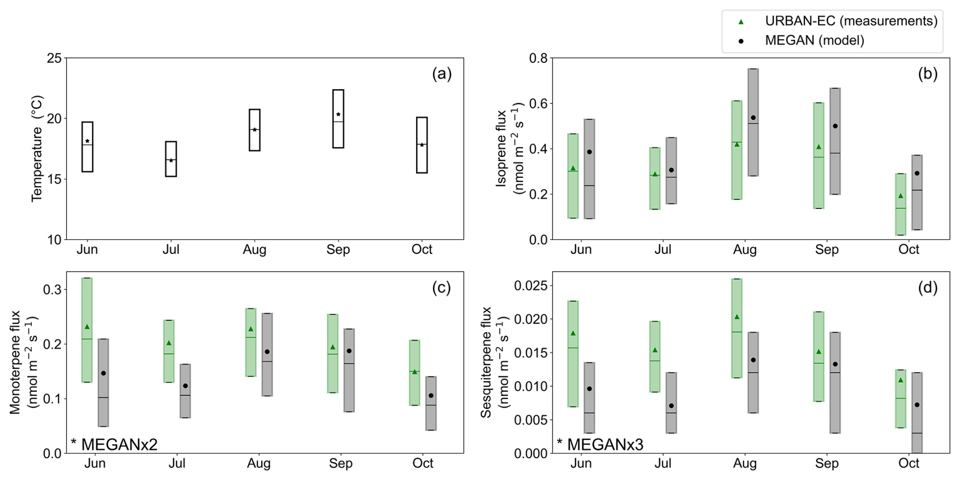
Figure 1 Daytime monthly statistics for (a) temperature, (b) isoprene flux, (c) monoterpene flux, and (d) sesquiterpene flux. Boxes represent the interquartile range, horizontal lines in the box represent the medians, and icons (stars, triangles, circles) represent the means. Shaded green boxes represent the measurements (URBAN-EC), and shaded grey boxes represent the biogenic emissions model (MEGAN). Note that for panels (c) and (d), MEGAN fluxes are scaled by a factor of 2 and 3, respectively.

Table 1 Average ± standard deviation of daytime (06:00–21:00) temperature, relative humidity (RH), photosynthetic photon flux density (PPFD), and footprint average ± standard deviation Normalized Difference Vegetation Index (NDVI) for each full month of flux data available and the entire study duration.

* The entire study NDVI is the average ± standard deviation of the result for each month.

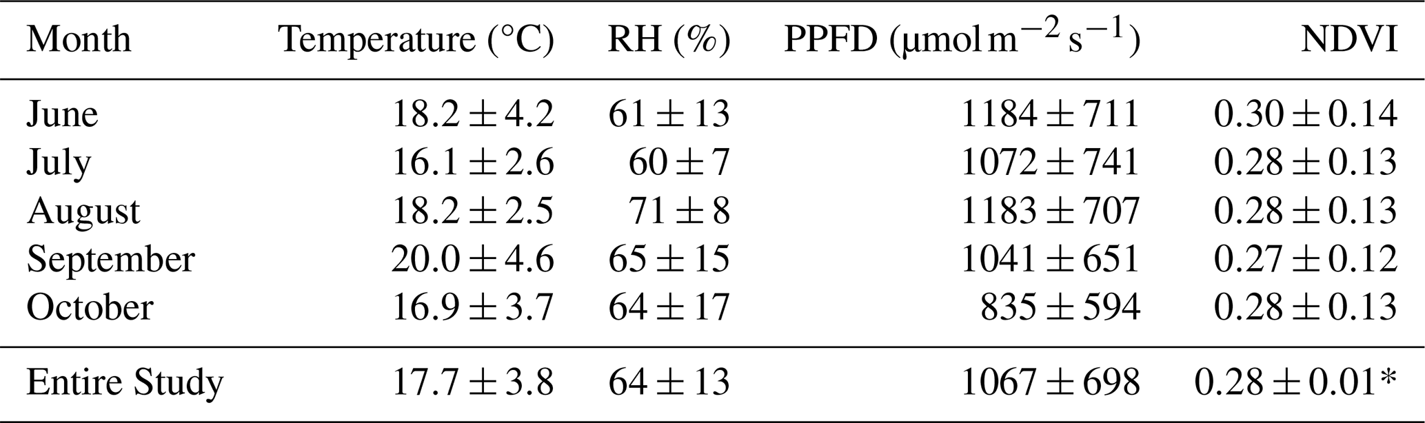
The 80 % URBAN-EC flux footprint extended about 1 km west of the tower. Berkeley city tree locations, June LAI, block scale population density, and the 80 % footprint-weighted flux maps of isoprene, monoterpenes, and sesquiterpenes can be seen in Fig. 2. Higher terpenoid fluxes were observed in the area west and directly southwest of the flux tower. This area is the commercial center of Downtown Berkeley and coincides with the lowest LAI values and some blocks with elevated population density. Although LAI measured by satellite is near zero in this area, there is an abundance of Berkeley city trees. The 2013 Berkeley city tree inventory (https://geodata.lib.berkeley.edu/catalog/berkeley-s7gq2s, last access: 13 March 2024) was used to understand the general spatial and species distribution of trees in the footprint, however, the inventory is only representative of trees on the street and in city parks. An emission rate for each species in the tree inventory was identified (Benjamin et al., 1996), and a species was deemed a high monoterpene or isoprene emitter if the emission rate was greater than 5 $\mathrm{\mu }\mathrm{g}(\mathrm{g}\mathrm{dry}\mathrm{leaf}{)}^{-\mathrm{1}}{\mathrm{h}}^{-\mathrm{1}}$. There are high isoprene and monoterpene emitting Berkeley city trees directly southwest of the flux tower in the region with low LAI, which could explain some of the isoprene and terpene fluxes from this region. Monoterpenes and sesquiterpene fluxes agreed spatially (R²=0.80 for their average footprint-weighted flux maps), indicating they likely have similar sources in the footprint. The R² between the footprint weighted flux maps of isoprene and monoterpenes was 0.59. Additional details on the spatial distribution of terpenoid fluxes will be discussed in Sect. 3.2.

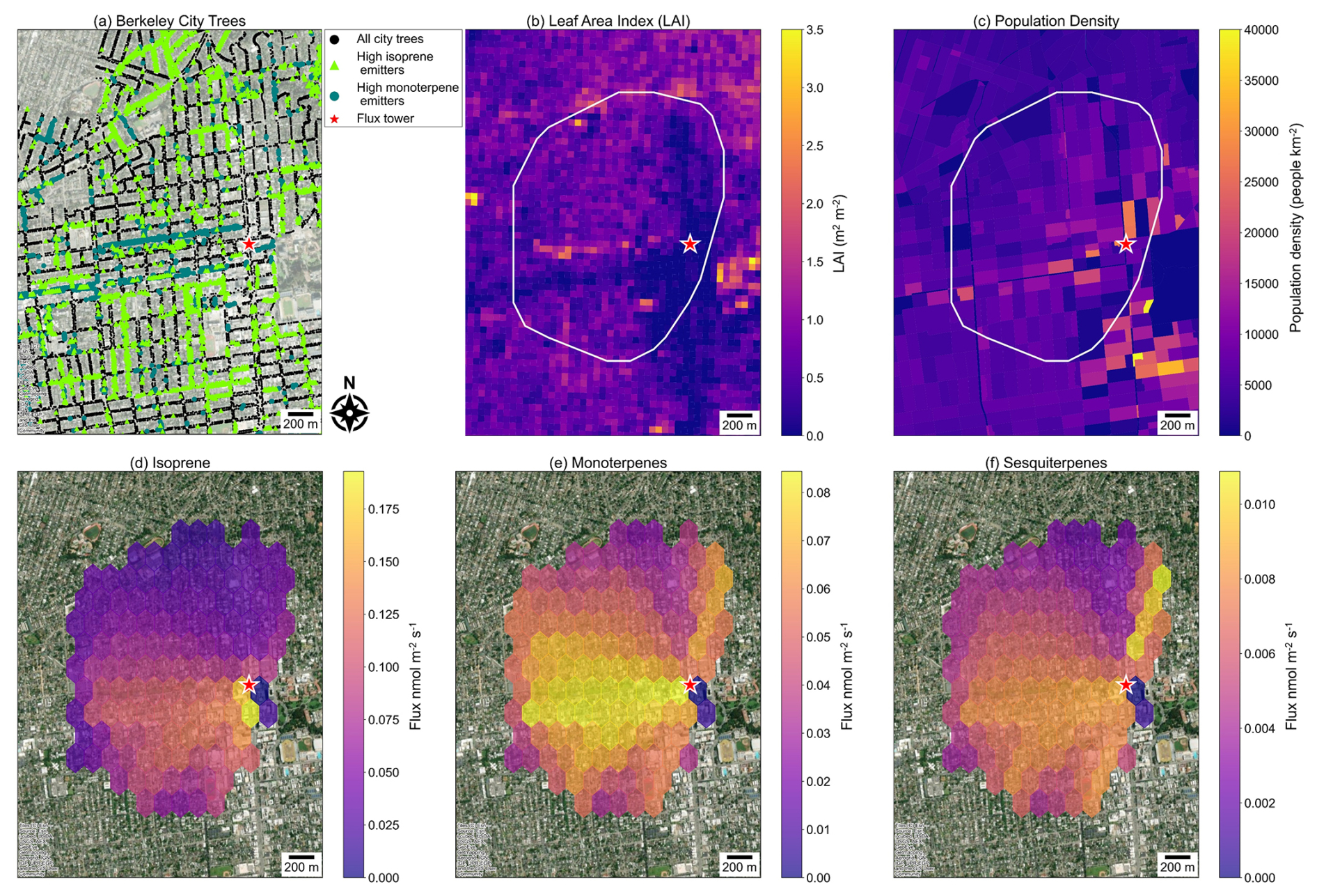
Figure 2 (a) Location of Berkeley city trees with high isoprene and monoterpene emitters indicated, (b) June leaf area index, (c) block scale population density, and 80 % footprint-weighted flux maps for (d) isoprene, (e) monoterpenes, and (f) sesquiterpenes. The URBAN-EC flux tower is represented by the red star icon. Each panel displays the same geographic area. The 80 % footprint is shown in (b) and (c) as the white trace. Map base layer is open source from ESRI World Imagery.

Despite being a small fraction (∼2 %) of the total measured daytime median molar VOC flux, isoprene, monoterpenes, and sesquiterpenes accounted for a substantial fraction of the median calculated OH reactivity flux (26 %) and secondary organic aerosol formation potential (SOAFP, 21 %) (Fig. 3). OH reactivity flux and SOAFP were calculated by scaling fluxes by the OH rate constant and SOA yield, respectively. VOCs with average measured molar flux contributions of over 0.05 % were included in Fig. 3. Coefficients used to calculate OH reactivity flux and SOAFP are from Pfannerstill et al. (2024), except for monoterpenes, which were based on the observed fraction of each isomer (see Sect. 3.2).

Isoprene comprised <2 % of the total measured VOC flux, 15 % of the total calculated OH reactivity flux, and 4 % of the total SOAFP. Similarly, monoterpenes were a small fraction (<2 %) of the total measured VOC flux, but they were more important for SOAFP (13 %) than OH reactivity flux (10 %). Sesquiterpene fluxes were the lowest among the terpenoids and made up <1 % of the measured flux, 1 % of the calculated OH reactivity flux, and 4 % of the calculated SOAFP. BVOCs are known to have outsized impacts on urban air quality due to their high reactivities despite having relatively low emission rates. These results are consistent with other cities (Acton et al., 2020; Gu et al., 2021; Pfannerstill et al., 2023).

Figure 3 Isoprene, monoterpene, and sesquiterpene fraction of the total measured (a) molar VOC flux, (b) calculated OH reactivity flux, and (c) calculated secondary organic aerosol formation potential (SOAFP) flux. The results shown represent the daytime median values (06:00–21:00). Percentages may not add up to 100 due to rounding.

The terpenoid fraction of the median total measured flux, calculated OH reactivity flux, and calculated SOAFP increased with increasing temperature (Fig. S5), which agrees with observations from Pfannerstill et al. (2024). At the highest observed temperatures (>25 °C), terpenoids accounted for 34 % of the calculated OH reactivity flux and 26 % of the calculated SOAFP. These relative contributions are lower than what was observed in Los Angeles (Pfannerstill et al., 2024), but still highlight the importance of temperature-dependent terpenoid emissions for the formation of secondary pollutants in urban environments. In present-day U.S. urban areas, particulate matter concentrations have a strong linear dependence on temperature, emphasizing the importance of understanding temperature dependent SOA precursors (Nussbaumer and Cohen, 2021; Vannucci and Cohen, 2022).

Observed terpenoid fluxes in Berkeley, summarized in Table 2, are generally comparable to other urban flux towers (Table 3). Parameters including the Normalized Difference Vegetation Index (NDVI), temperature, and population density can inform differences in observed urban terpenoid fluxes, and values for Berkeley are reported in Table 1 and below. NDVI, which provides a measure of the health and density of vegetation, was calculated using the Sentinel-2 (Copernicus Sentinel-2 (processed by ESA), 2021) near infrared and red bands (bands 8 and 4) at 50 m resolution. One mean NDVI was acquired for the footprint for each month, and the value ranged from 0.27 to 0.30 (Table 1). The residential population density in the URBAN-EC footprint is ∼6500 people km⁻², though the true population density is temporally variable due to commuters and visitors in this urban area.

Table 2 Daytime flux and mixing ratio statistics for isoprene, monoterpenes, and sesquiterpenes. 25th, 50th, and 75th percentiles are shown with the mean and standard deviation.

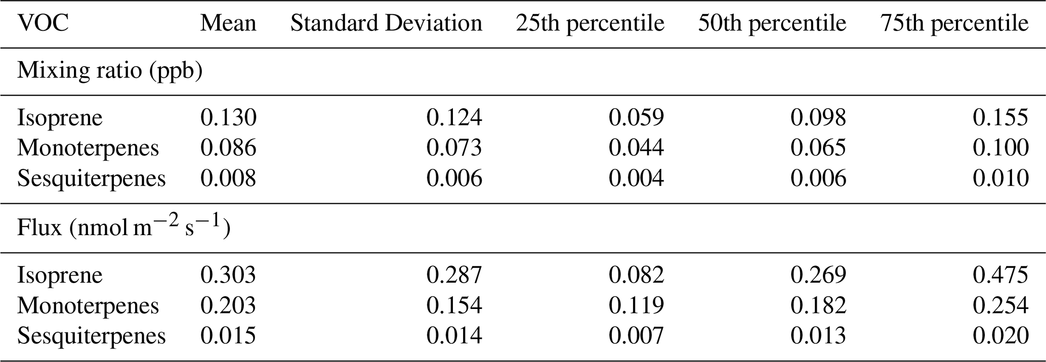
Table 3 Summary of urban fluxes of isoprene, monoterpenes, and sesquiterpenes from Berkeley, California (this study) and others reported in the available literature.

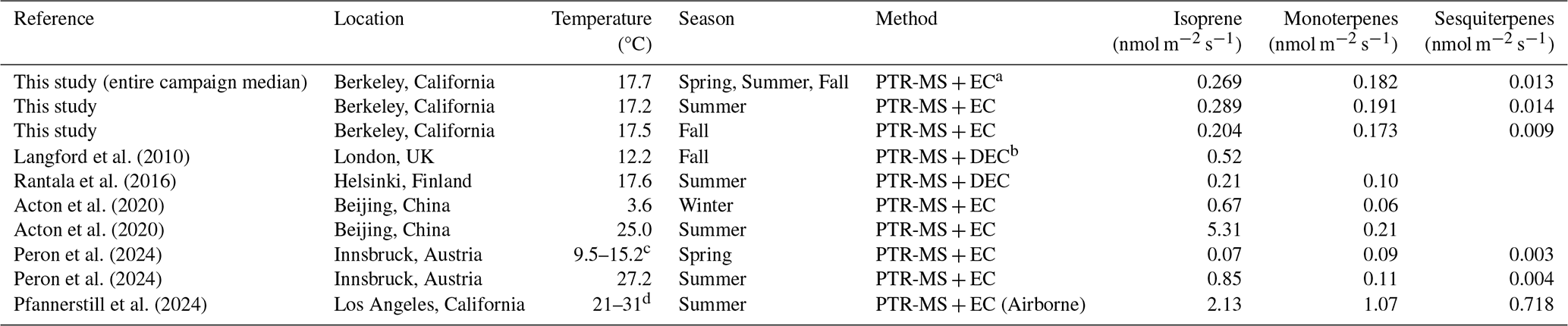
^a EC = eddy covariance; ^b DEC = disjunct eddy covariance; ^c Range of average temperatures in 2018, 2020, and 2021; ^d Range of median flight temperatures

The daytime median isoprene mixing ratio was 0.098 ppb (interquartile range (IQR): 0.059–0.155 ppb), and the median flux was 0.269 nmol m⁻² s⁻¹ (IQR: 0.082–0.475 nmol m⁻² s⁻¹). Isoprene fluxes in Berkeley were close to observations from Innsbruck, Austria (Peron et al., 2024), Helsinki, Finland (Rantala et al., 2016), and London, UK (Langford et al., 2010), and are about an order of magnitude lower than isoprene fluxes in Los Angeles, California (Pfannerstill et al., 2024) and Beijing, China (Acton et al., 2020). Temperature must be considered when comparing terpenoid fluxes because of its impact on their emission. Los Angeles and Beijing, which had the highest terpenoid fluxes, had higher temperatures compared to Berkeley.

The daytime median monoterpene mixing ratio was 0.065 ppb (IQR: 0.044–0.100 ppb), and the median flux was 0.182 nmol m⁻² s⁻¹ (IQR: 0.119–0.254 nmol m⁻² s⁻¹). Monoterpene fluxes in Berkeley were similar to those in Innsbruck, Austria (Peron et al., 2024), Helsinki, Finland (Rantala et al., 2016), and Beijing, China (Acton et al., 2020) but lower than those in Los Angeles, California (Pfannerstill et al., 2024).

Urban sesquiterpene fluxes are more sparsely reported in the literature than monoterpenes and isoprene. The sesquiterpene daytime median mixing ratio was 0.006 ppb (IQR: 0.004–0.010 ppb), and the median flux was 0.013 nmol m⁻² s⁻¹ (IQR: 0.007–0.020 nmol m⁻² s⁻¹). Sesquiterpene fluxes in Berkeley were about a factor of three higher than those in Innsbruck, Austria (Peron et al., 2024), and almost two orders of magnitude lower than Los Angeles, California (Pfannerstill et al., 2024). Temperature and source differences are likely to play an important role in monoterpene and sesquiterpene flux comparisons.

3.2 Terpene sources

Weekday versus weekend differences are an indicator of anthropogenic activity and can provide useful bounding of the biogenic and anthropogenic contributions to terpenoid fluxes. Under similar meteorological conditions, BVOC emissions are not expected to be different on weekdays compared to weekends. Interestingly, weekday daytime temperatures were 0.7 °C (4 %) higher on average (p<0.05) due to occurrences of hotter periods on weekdays, however, this difference was too small to produce extraneous BVOC emissions. There was not a statistically significant difference in isoprene fluxes between weekdays and weekends (p>0.05), while monoterpenes and sesquiterpenes were significantly higher on weekdays compared to weekends (p<0.05). Weekday fluxes of monoterpenes and sesquiterpenes were on average 24 % higher than weekend fluxes on a 24 h basis, and larger differences were observed during the morning (55 % and 56 %, respectively). These morning enhancements are shown in Fig. 4.

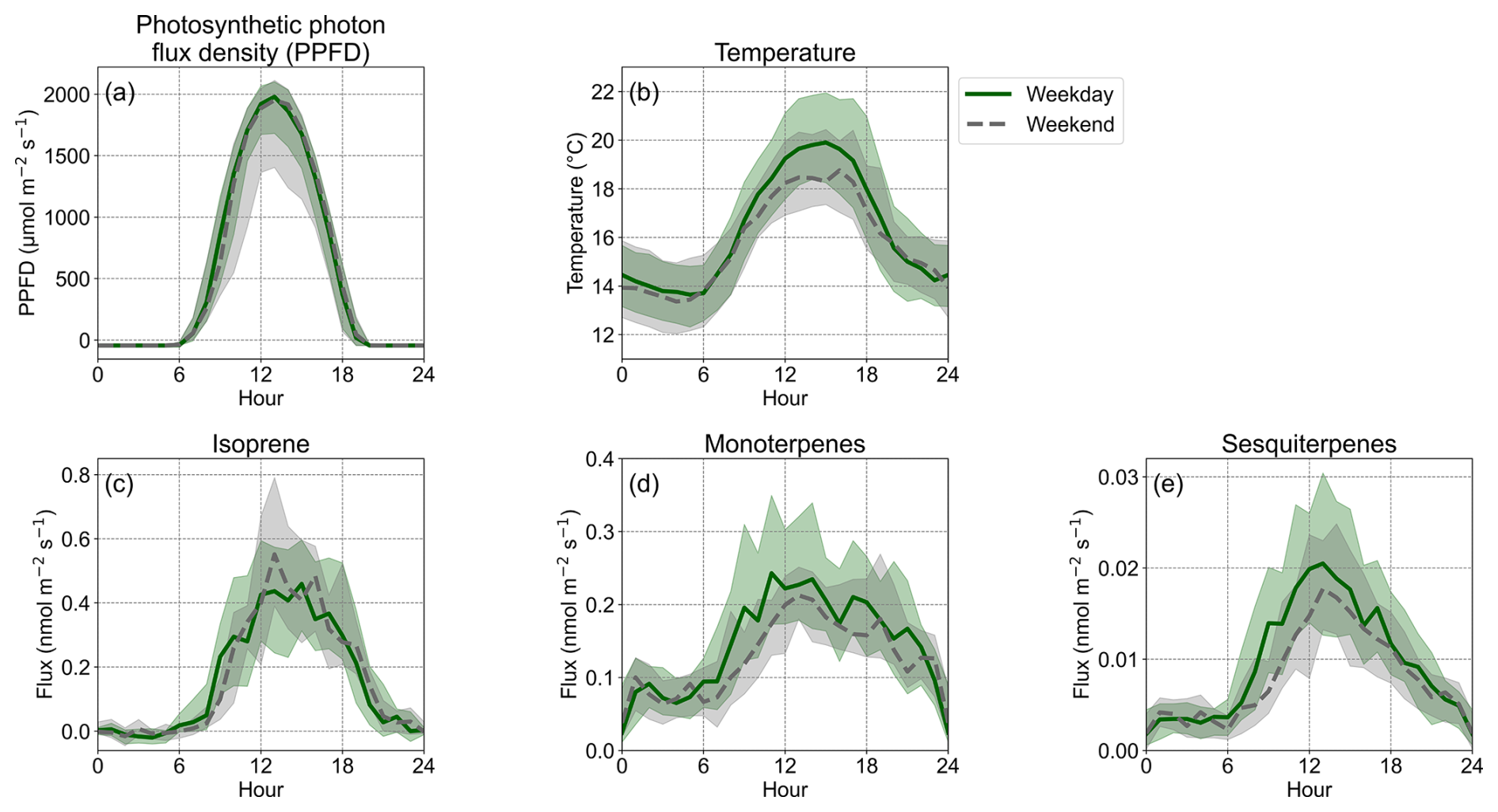
Figure 4 Diurnal (a) photosynthetic photon flux density (PPFD), (b) temperature, and fluxes of (c) isoprene, (d) monoterpenes, and (e) sesquiterpenes. Data are split by weekday (green solid lines) and weekend (grey dashed lines). Lines represent the median and the shaded region represents the interquartile range for each hour.

Differences in the oxidizing capacity of the urban atmosphere from weekdays to weekends were not expected to impact the comparisons. At most, average ozone concentrations were 2 ppb higher on weekends compared to weekdays. The greatest difference was observed in the morning (06:00 to 11:00: weekdays: 21.5 ppb, weekends: 23.2 ppb), while the difference was negligible when averaging over 24 h (weekdays: 24.2 ppb, weekends: 24.7 ppb). To assess the potential for chemical loss to impact weekday/weekend comparisons, first, emission velocities were used to understand the lifetime of each terpenoid relative to the others. The emission velocity was calculated using the ratio of the median flux to the median concentration, and was 6.3, 6.5, and 4.9 cm s⁻¹ for isoprene, monoterpenes, and sesquiterpenes, respectively. The similar velocities between isoprene and monoterpenes indicate that they have similar lifetimes, while the sesquiterpene lifetime may be slightly longer. The lifetime for isoprene was 2.6 h using the measured ozone concentration (24 ppb) and an assumed OH concentration of 1.0×10⁶ molecules cm⁻³, and the lifetime of the sum of measured monoterpene isomers is expected to be similar because of the similar emission velocities. Under these conditions, the measured sesquiterpene isomers likely have lifetimes similar to cedrene (3.3 h under these conditions). An important caveat to this analysis is that the concentration measurement is impacted by a larger area than the flux footprint. The chemical lifetimes were compared to turbulent transport timescales from the surface to the tower. Turbulent timescales for the URBAN-EC tower are ∼100 s based on the ratio of measurement height to u*. Following the analysis presented by Kaser et al. (2022), on this turbulent time scale, assuming cedrene-like sesquiterpenes were present, weekday and weekend terpenoid losses to OH and ozone reactions were less than 1 % (Kaser et al., 2022). If we assume more reactive sesquiterpenes were present, like beta-caryophyllene, weekday losses would be 51 % and weekend losses would be 54 %. These differences are too low to produce the observed weekday versus weekend differences observed.

3.2.1 Isoprene

Weekday and weekend isoprene diurnal fluxes had overlapping interquartile ranges and medians for most hours of the day (Fig. 4), and their averages were not significantly different (p>0.05). Isoprene fluxes followed a diurnal trend similar to PPFD and were in agreement with the expected diurnal trend for biogenic isoprene emissions (Figs. 4, S6). Additionally, the distributions of measured and MEGAN isoprene fluxes agree across months (Fig. 1). Measured isoprene fluxes were also consistent with the expected relationship with temperature, assuming biogenic emissions (Fig. S7). The agreement between the measured and modeled biogenic isoprene temporal trends, both seasonally and diurnally, indicates the factors driving isoprene emissions in MEGAN (temperature, PPFD, LAI, etc.) are also likely also driving the observed trends. Although the median and IQR of the temporal trends for URBAN-EC and MEGAN agree, the overall correlation is low (R²=0.26). The central tendencies of the data agree, but the R² is low due to considerable scatter and variability in the ∼6 months of field and modeled data.

The similarity between weekday and weekend emissions and agreement with expected biogenic trends suggests that isoprene emissions in the URBAN-EC footprint are predominantly from biogenic sources. These results are contrary to a few prior studies. In Innsbruck Austria, Peron et al. (2024) observed an average weekday versus weekend difference for isoprene and attributed this difference to anthropogenic sources, particularly, vehicles. Other studies have also identified anthropogenic isoprene emissions from traffic in urban environments (Borbon et al., 2001; Wernis et al., 2022). These differences could be attributed to different fuel types in different cities and the prevalence of heavy duty versus light duty vehicles. The footprint does not contain highways or industrial areas, so any vehicle isoprene emissions would likely be small compared to the biogenic emissions. Further, at night, when biogenic isoprene emissions were not expected, a correlation was not found between isoprene and benzene fluxes, a tracer for vehicular emissions. However, we cannot rule out minor contributions from anthropogenic isoprene sources that are small relative to the biogenic emissions or have similar activity patterns on weekdays and weekends.

3.2.2 Monoterpenes

To evaluate anthropogenic and biogenic contributions to monoterpene fluxes, weekday and weekend data were analyzed in discrete temperature bins (Fig. 5). This analysis was employed here to understand the cause of weekday versus weekday differences without potential impacts of slightly higher weekday temperatures. Each bin spans 2 °C and the data ranges from 12 to 22 °C. These parameters were chosen to ensure each bin had sufficient data. Each weekday temperature bin had approximately the same temperature distribution as its corresponding weekend bin (Table S6). Therefore, differences in weekday and weekend fluxes within a bin can be attributed to temperature-independent sources, like differing anthropogenic sources or potential changes in flux footprint area.

Across bins as a function of temperature, the mean, 75th percentile, and 95th percentile were consistently higher for the weekday than weekend monoterpene fluxes (Fig. 5). The difference within bins must be attributed to variations in anthropogenic emissions, because temperature, the main driver for biogenic terpene emissions, is constrained. The modeled monoterpene fluxes displayed the expected exponential relationship with temperature (β=0.11 K⁻¹), while measured monoterpene fluxes had a weaker exponential relationship (β=0.05 K⁻¹) (Fig. S8). An important, temperature-independent anthropogenic source is likely responsible for the dampened exponential temperature relationship, particularly the elevated monoterpene fluxes at low temperatures. Similar results were reported for Canadian cities (Jo et al., 2023). The R² between URBAN-EC and MEGAN monoterpene fluxes was very low at 0.07, further indicating that non-biogenic sources contributed to the observations.

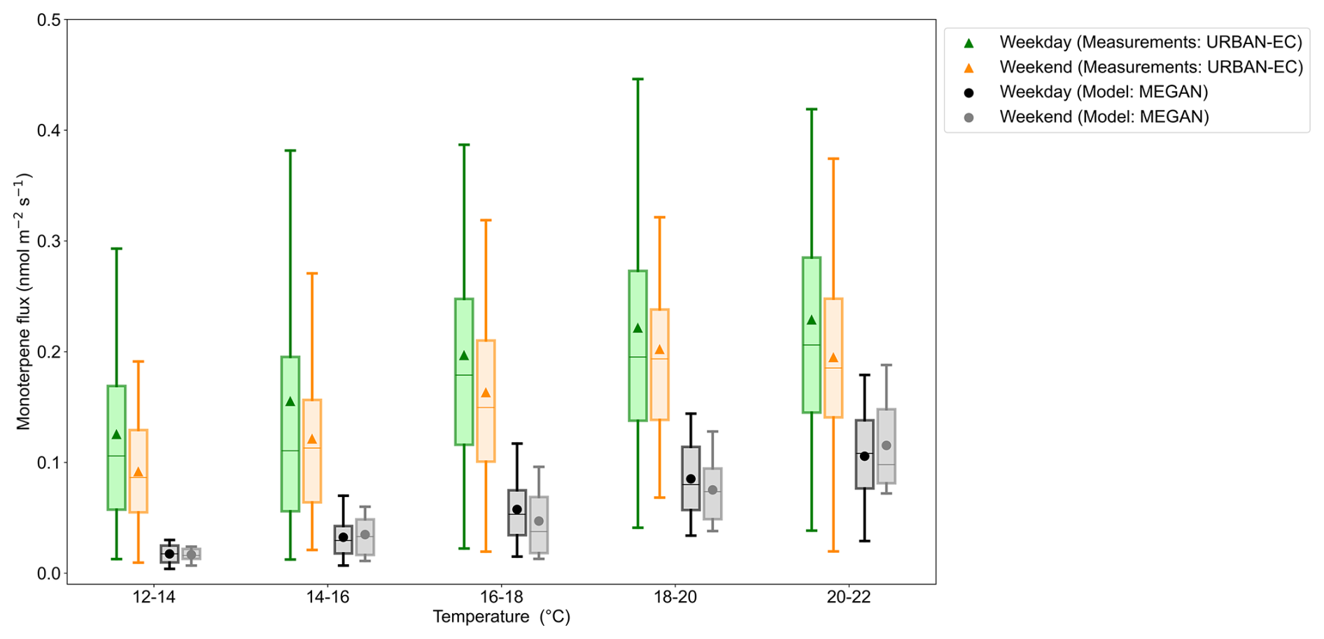
Figure 5 Measured (URBAN-EC) and modeled (MEGAN) monoterpene fluxes binned by temperature. Each bin spans 2 °C. Data are split into weekday and weekend fluxes. Boxes are plotted against the midpoint temperature of each bin with an offset for clarity. Triangle (URBAN-EC) and circle (MEGAN) icons represent the means, boxes represent the interquartile ranges, horizontal lines in the boxes represent the medians, and capped vertical lines represent the 5th and 95th percentiles. Data are averaged so that MEGAN and URBAN-EC fluxes are at the same time resolution (1 h), and only time periods where both datasets are available are included for a direct comparison (hours from 05:00 to 18:00).

The weekday versus weekend ratio is highest at lower temperatures for the mean, median, and 75th percentile, and this ratio decreased with increasing temperature (Fig. S9). The decreasing trend for the mean and 75th percentile within temperature bins shows that high weekday anthropogenic emissions events are likely to occur at lower temperatures, which typically correspond to morning hours (Fig. 4, Table S6). Biogenic emissions are expected to be the highest in the afternoon when the temperature is the highest. Therefore, lower weekday to weekend ratios in higher temperature bins is likely a feature of both biogenic emissions being higher and episodic anthropogenic emissions dominantly occurring during cooler morning hours. The diurnal trend of monoterpenes also shows the greatest deviation between the weekday and weekend data during morning and early afternoon (Fig. 4).

Within each temperature bin, the mean to median ratio is greater than one, which shows there is an abundance of episodic high-emission events (Fig. S9). The mean to median ratio is indicative of the degree of high, episodic emission events because the mean is more sensitive to these data points than the median. The ratio is higher for weekdays compared to weekends for all bins except one (Fig. S9), showing that weekday fluxes have greater influence from episodic high-emission events (expected from anthropogenic sources) regardless of ambient temperature. This is also corroborated by the higher weekday means, 75th, and 95th percentiles relative to weekends in all temperature bins (Fig. 5).

The excess weekday anthropogenic monoterpene flux can be estimated by subtracting the weekend flux from the weekday flux while accounting for minor changes in biogenic emissions. The measured flux (F) is composed of biogenic (F_bio) and anthropogenic (F_anth) fluxes. As shown below (Eq. 3), the difference between the weekday and weekend fluxes (F_wDay−wEnd) is composed of the difference between weekday and weekend F_bio and F_anth. The biogenic flux difference is included to account for slight deviations in temperature between weekdays and weekends.

$$\begin{array}{}\text{(3)}& \begin{array}{rl}{F}_{\mathrm{wDay}-\mathrm{wEnd}}& =\mathrm{\Delta }{F}_{\mathrm{bio}}+\mathrm{\Delta }{F}_{\mathrm{anth}}\\ & =\left(F_{\mathrm{bio},\mathrm{wDay}}-F_{\mathrm{bio},\mathrm{wEnd}}\right)\\ & +\left(F_{\mathrm{anth},\mathrm{wDay}}-F_{\mathrm{anth},\mathrm{wEnd}}\right)\end{array}\end{array}$$

F_bio is calculated using the observed standard emission rate (M_s), standard temperature (T_s), observed temperature (T_wDay or T_wEnd), and β of 0.10 K⁻¹ (typical for biogenic emissions of monoterpenes) (see Eq. 2). M_s is the median of the weekend flux observations between 296 and 300 K. The weekend data were used because lower anthropogenic terpenoid emissions were expected. Solving for ΔF_anth yields Eq. (4).

$$\begin{array}{}\text{(4)}& \begin{array}{rl}\mathrm{\Delta }{F}_{\mathrm{anth}}& =F_{\mathrm{wDay}-\mathrm{wEnd}}-\left[M_{\mathrm{s}}\exp \left(\mathit{\beta }\left(T_{\mathrm{wDay}}-T_{\mathrm{s}}\right)\right)\right.\\ & \left.-M_{\mathrm{s}}\exp \left(\mathit{\beta }\left(T_{\mathrm{wEnd}}-T_{\mathrm{s}}\right)\right)\right]\end{array}\end{array}$$

This method provides the excess weekday anthropogenic monoterpene flux, or ΔF_anth, which is the lower bound of the anthropogenic monoterpene emission. It is not a measure of the total anthropogenic emission, as anthropogenic monoterpene emissions are expected on both weekdays and weekends which are not accounted for here. ΔF_anth was calculated for isoprene using the same method, except accounting for biogenic isoprene using both temperature and light dependence (Guenther et al., 1993).

The excess weekday anthropogenic monoterpene fraction (ΔF_anth divided by observed weekday monoterpene flux) and flux were calculated for daytime hours. ΔF_anth varied by time of day; the highest contribution from anthropogenic sources was during the morning (Fig. 6). At most, the excess weekday anthropogenic monoterpene flux was 47 % and 46 % of the total observed monoterpene flux at 06:00 and 09:00, respectively. Measured monoterpene fluxes peaked in the morning before biogenic monoterpene emissions were expected to increase (Fig. S6), which further supports that there is an important anthropogenic monoterpene source in the morning. After 12:00, when the temperature and biogenic monoterpene emissions were highest, the excess weekday anthropogenic fraction leveled off at ∼25 %. On average, the daytime excess weekday anthropogenic fraction of monoterpene emissions was 23 % of the total weekday flux. The total anthropogenic fraction of monoterpene emissions is expected to be higher, but it cannot be calculated using this method.

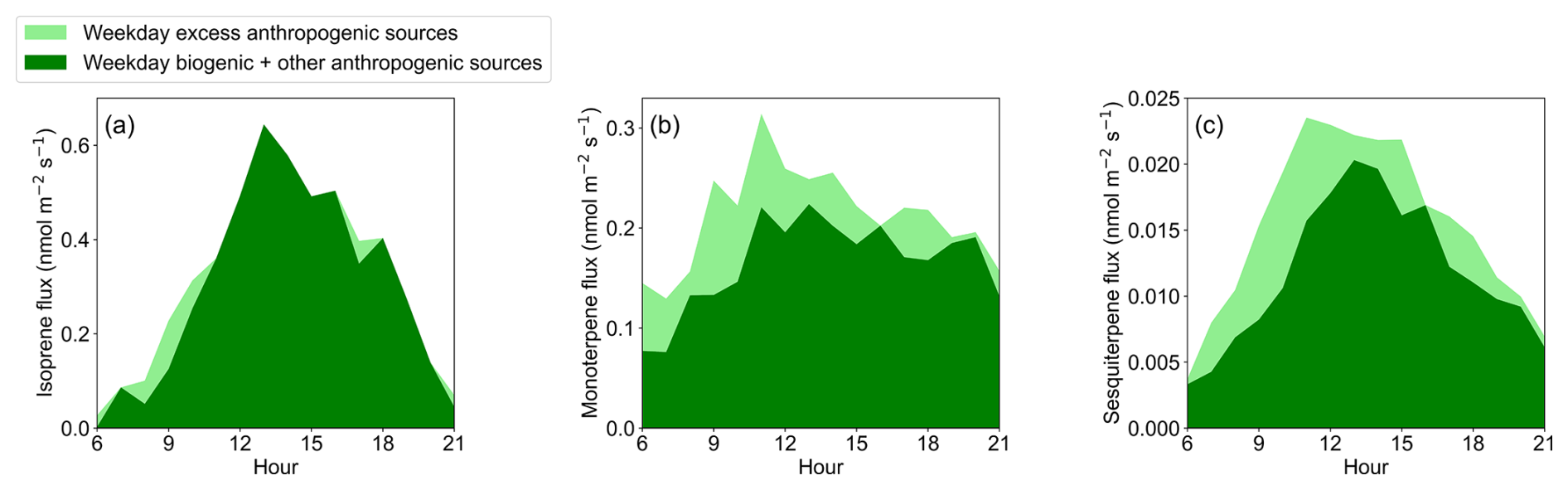
Figure 6 Weekday fluxes of (a) isoprene, (b) monoterpene, and (c) sesquiterpenes during daytime hours. Data are separated by weekday excess anthropogenic sources (ΔF_anth) and weekday biogenic + other anthropogenic sources and are stacked to represent the total flux.

Unlike monoterpenes and sesquiterpenes, the weekday excess anthropogenic fraction of isoprene emissions is close to zero. Figure 6 shows that there could be a small contribution from weekday excess sources of isoprene in the morning and around 17:00, consistent with higher traffic times. Sesquiterpene trends will be discussed in the next section.

Other urban VOC studies have estimated the anthropogenic fraction of monoterpene emissions and reported a similar range. Anthropogenic sources contributed 26 % and 53 % of the monoterpene mixing ratio in summer and winter, respectively, in Atlanta, Georgia, as determined by non-negative matrix factorization (Peng et al., 2022). In Innsbruck, Austria, the average weekday to weekend ratio was used to determine the fraction of anthropogenic monoterpene flux. 43 % of springtime monoterpene fluxes and less than 20 % of summertime monoterpene fluxes were described as anthropogenic using this method (Peron et al., 2024). Combined modeling and flux data from Beijing resulted in an anthropogenic monoterpene fraction of 65 % in the urban core (Xie et al., 2025). The monoterpene area emission rate from VCPs in New York City was 1.3 to 2.1 nmol m⁻² s⁻¹ (Coggon et al., 2021), which is about an order of magnitude higher than the total (biogenic + anthropogenic) monoterpene area emission rate reported here. The higher anthropogenic area emission rate in New York City is likely due to the population density being $\sim \mathrm{7}\times$ higher than Berkeley.

The anthropogenic emissions inventory, FIVE-VCP, includes monoterpene emissions from VCPs. Unlike observations, FIVE-VCP has consistent weekday and weekend emissions, and FIVE-VCP monoterpene emissions are stable throughout the months when the inventory is available (Fig. S10). We determined the total modeled emission by adding the contributions of anthropogenic (FIVE-VCP) and biogenic (MEGAN) monoterpene emissions. The correlation coefficient (R²) between URBAN-EC and total modeled fluxes was low at 0.09, a minor improvement from the comparison with MEGAN alone (Fig. S11). These comparisons show that the magnitude, temporal pattern, and weekday/weekend differences of urban monoterpene emissions are not captured by MEGAN and FIVE-VCP at this location.

Comparing the timing of fluxes of monoterpenes to D5 siloxane can provide insight into the potential for consumer products to influence the observed trends. D5 siloxane is an ingredient in antiperspirant, and has been identified as a tracer for personal care products (Gkatzelis et al., 2021a). D5 siloxane fluxes peak at 08:00 on weekdays and 11:00 on weekends during URBAN-EC, highlighting differences in foot traffic and/or personal care product use patterns from weekdays to weekends (Fig. S12). This timing is consistent with the peak in weekday excess anthropogenic monoterpene emission. High emissions of D5 siloxane typically occur in the morning and decline throughout the day due to application and evaporation of personal care products (Coggon et al., 2018; Tang et al., 2015). While the D5 weekday to weekend differences show the potential for varying VCP use patterns on weekdays and weekends, we do not expect personal care products to be the dominant source of anthropogenic monoterpene emissions. The average emissions of D5 and monoterpenes were not collocated spatially (R²=0.60, Fig. S13) or temporally (R²=0.31). Additionally, monoterpenes and D5 were not correlated in studies of personal care product use in indoor environments (Arata et al., 2021; Tang et al., 2015, 2016). Terpenoids have been detected in the headspace of some personal care products (Steinemann et al., 2011); however, these products may not also include D5 siloxane. Further, monoterpene emissions from applied personal care products range from 2.5 to 4.8 mg per person d⁻¹ (Tang et al., 2016; Stönner et al., 2018; Arata et al., 2021), while the anthropogenic monoterpene emission rate in the URBAN-EC footprint ranges from 83 to 360 mg per person d⁻¹ (assuming the observed monoterpene flux is 23 % to 100 % anthropogenic and a footprint average population density of 6500 people km⁻²). Comparing these emission factors indicates that at most, ∼6 % of the anthropogenic monoterpene emissions can originate from personal care products.

Other fragranced products like cleaning supplies, which are known indoor sources of monoterpenes, may be important contributors to the observed anthropogenic monoterpene emissions (Arata et al., 2021; Steinemann et al., 2011; Sweet et al., 2025). These emissions can escape to the outdoors, and the products likely have weekday/weekend differences in use, particularly in commercial applications. Cooking has reliable tracers including nonanal and octanal (Coggon et al., 2024b), but these VOCs did not exhibit a statistically significant weekday/weekend difference (p>0.05), suggesting cooking does not drive the observed monoterpene weekday/weekend differences. Assuming cooking and building material sources of monoterpenes do not vary from weekdays to weekends, we assume that the observed variability is driven by different use patterns of other fragranced consumer products such as cleaning supplies.

Limonene is considered a tracer for anthropogenic monoterpene emissions due to its prevalence in fragranced consumer products, though it is also emitted by plants (Geron et al., 2000; Steinemann et al., 2011; Gkatzelis et al., 2021a). Other monoterpenes including alpha and beta pinene are also emitted by fragranced consumer products (Link et al., 2024; Zannoni et al., 2025). Sorbent tubes and 2D GCMS analysis were deployed for three days in June of 2022 to provide a snapshot of the monoterpene speciation in Berkeley. Limonene accounted for 19 % of the monoterpene mixing ratio (Fig. S14). The prevalence of other monoterpenes including alpha-pinene (35 %), beta-myrcene (16 %), (+)-3-carene (13 %), beta ocimene (12 %), and beta-pinene (4 %) indicate that biogenic emissions were also an important source of monoterpenes on average. During winter in New York City, limonene accounted for a higher fraction (53 %) of the monoterpene mixing ratio, caused in part by both the loss of deciduous leaf cover (i.e., lower biogenic emissions in winter) and higher population density (Coggon et al., 2021). The measured limonene fraction at 19 % suggests the anthropogenic contributions to monoterpenes in the region around URBAN-EC are more limited than New York City. Because the 2D GCMS analysis represents mixing ratios rather than fluxes, the observations reflect contributions from a larger geographic area than the flux footprint because of regional transport.

High monoterpene fluxes west of the flux tower correspond with the locations of Ohlone park, a city greenspace, and University Avenue, a highly populated commercial corridor (Fig. 2). Additionally, high monoterpene fluxes were observed from the northeast, which corresponds to blocks with high population density in addition to a plant growing facility managed by the College of Natural Resources at the University of California, Berkeley (Fig. 2). The collocation of areas with high population density and urban greenspaces, along with the lower number of datapoints from the north makes disentangling the emissions sources difficult. Figure 2 shows that monoterpene and sesquiterpene fluxes have a similar spatial distribution, indicating they have some similar sources in the footprint. The correlation coefficient (R²) between the time series of fluxes of monoterpenes and sesquiterpenes was 0.51, while their footprint weighted-flux maps had an R² of 0.80.

3.2.3 Sesquiterpenes

There was a statistically significant difference between weekday and weekend fluxes of sesquiterpenes (p<0.05), indicating the presence of anthropogenic sources. The expected biogenic emissions change due to the average temperature change of 0.7 °C was negligible compared to the average weekday versus weekend flux difference (i.e., using T=0.7 °C and β=0.17 K⁻¹ in Eq. (2) with the observed M_s values resulted in an emission difference of less than 10⁻²⁵ nmol m⁻² s⁻¹). The median weekday and weekend diurnal profiles for sesquiterpenes were similar, except weekday fluxes were slightly elevated (Fig. 4). Sesquiterpene fluxes reached a maximum just after 12:00 and decreased slowly until leveling off overnight. Sesquiterpene fluxes studied here were about an order of magnitude lower than isoprene and monoterpene fluxes, consistent with prior studies (Kaser et al., 2022).

Sesquiterpenes fluxes were analyzed in discrete temperature bins using the same methods described above for monoterpenes, and similar results were found (Fig. S7). For all bins, the mean, 75th, and 95th percentiles were higher for weekday fluxes than weekend. These consistent results across temperature bins indicates that anthropogenic sources drive the weekday to weekend differences as opposed to temperature-driven biogenic emissions. MEGAN sesquiterpene fluxes in each temperature bin did not follow this trend.

The excess weekday anthropogenic sesquiterpene emissions were calculated while accounting for changes in temperature-driven biogenic sesquiterpene emissions. ΔF_anth was calculated for sesquiterpenes as it was for monoterpenes, except a β of 0.17 K⁻¹ was used (Guenther et al., 2012). The excess weekday anthropogenic sesquiterpene fraction followed a similar trend to that of monoterpenes (Fig. 6), where the largest anthropogenic fractions occurred in the morning. Measured sesquiterpene fluxes also increased in the morning before modeled biogenic fluxes (Fig. S6), indicating an important anthropogenic source of sesquiterpenes in the morning. On average, the weekday excess anthropogenic fraction was 24 %, which is expected to be the lower-bound estimate of the total anthropogenic fraction. Peron et al. (2024) who analyzed terpenoid weekday versus weekend fluxes in Innsbruck, Austria, did not see a significant difference for sesquiterpenes (Peron et al., 2024). Currently, reports of anthropogenic sources of sesquiterpenes to urban environments are limited. Anthropogenic sources of sesquiterpenes include fragrances, cooking (Klein et al., 2016), and incense (Ofodile et al., 2024). Essential oils contain sesquiterpenes and oxygenated sesquiterpenes (Moniodis et al., 2017; Todorova et al., 2023). There could be overlapping anthropogenic sesquiterpene and monoterpene sources in Berkeley, as indicated by similar spatial emission patterns (Fig. 2) and similar deviations between the diurnal trends of observed and MEGAN fluxes (Fig. S6).

4 Conclusions

This study highlights the importance of terpenoids for urban atmospheric chemistry by describing their emissions, source apportionment, and impact on secondary pollutant formation. Direct measurements of terpenoid emissions in urban environments are rare, especially longer duration studies, despite their importance for validating bottom-up emissions inventories and models such as FIVE-VCP and MEGAN. We presented isoprene, monoterpene, and sesquiterpene fluxes in Berkeley, California from May to November of 2022. Isoprene and monoterpene median fluxes were 0.269 and 0.182 nmol m⁻² s⁻¹, respectively, while sesquiterpene fluxes were about an order of magnitude lower at 0.013 nmol m⁻² s⁻¹. Median fluxes reported here were similar to most prior urban flux studies with similar temperature ranges, and this comparison helps constrain expected urban terpenoid fluxes. Terpenoids comprised a small fraction of the total measured VOC flux (∼2 %), but an important fraction of the OH reactivity (26 %) and SOA formation potential (21 %), highlighting their important role in urban atmospheric chemistry for air pollution formation and the necessity of accurately understanding their sources.

Weekday versus weekend flux differences were used to determine if anthropogenic sources impacted terpenoid emissions. Isoprene did not exhibit a weekday/weekend difference, indicating that it had predominantly biogenic sources or small anthropogenic sources that were similar on weekdays and weekends. The observed distribution of isoprene fluxes agreed with modeled biogenic isoprene fluxes temporally, indicating that the factors which drive isoprene emissions in MEGAN (i.e., temperature, PPFD, LAI, etc.) likely caused the observed fluxes. The landscape average isoprene emission factor of 4.56 nmol (m² leaf area)⁻¹ s⁻¹ determined for this site indicates that the average isoprene emission for these trees is about a factor of two lower than the MEGAN global-average value for broadleaf deciduous trees. Future studies that compare measured and modeled urban terpenoid emissions should also examine the suitability of the urban tree emission factors used in biogenic VOC models.

Monoterpenes and sesquiterpenes had statistically significant weekday/weekend differences, and the excess weekday anthropogenic emission fractions were 23 % and 24 %, respectively, representing a lower bound of the total anthropogenic fraction. FIVE-VCP, an anthropogenic emissions inventory, did not include weekday/weekend differences for monoterpenes. Monoterpenes and sesquiterpenes had higher anthropogenic emission fractions in the morning, and their fluxes deviated from modeled biogenic emissions temporal trends during these hours, further indicating important weekday morning anthropogenic sources. The anthropogenic emission fraction was lower in the afternoon when temperature-driven biogenic emissions were high. Volatile chemical products, including fragranced cleaning products, are thought to be responsible for most of the excess weekday anthropogenic terpene emissions. Personal care products are expected to be a minor source of anthropogenic monoterpenes. The anthropogenic monoterpene and sesquiterpene sources are likely different from isoprene sources based on differences in the diurnal patterns between MEGAN and measured fluxes and different spatial distributions.

The analysis presented here contributes to an improved understanding of reactive VOCs and precursors to secondary pollutants in urban environments. Terpenoids have consistently been identified as important contributors to OH reactivity and SOA formation both here and in prior studies (e.g., Pfannerstill et al., 2024), and as a result, they are potential targets for emissions reductions. The biogenic fraction of terpenoid emissions was higher than the estimated anthropogenic fraction at this site during the measurement period. Planting low terpenoid emitting trees may be an effective way to reduce secondary pollutant precursor emissions in the future as existing city trees need to be replaced. Additionally, decreased use of terpenoid compounds in fragranced consumer products would likely decrease terpenoid emissions from anthropogenic sources in urban environments.

Further work on terpenoid source apportionment in urban environments would contribute to a better understanding of pollutant formation associated with consumer product use. Given the disagreement in modeled and measured monoterpene emissions, further work is also needed to constrain biogenic and anthropogenic emissions models and inventories for terpenoids in urban locations. Comparing direct observations of terpenoid fluxes like these with bottom-up approaches in urban environments will contribute to more robust models, and therefore, more accurate air quality predictions. The importance of terpenoids for urban atmospheric chemistry will grow in a warming planet due to their temperature dependent emission and resulting impact on OH reactivity and SOA formation. Additional investigation of terpenoid fluxes in other urban environments plus characterization of direct sources of anthropogenic terpenoids is warranted.