Biomass burning aerosol radiative effects in the Southeast Atlantic depend strongly on meteorological forcing method

Biomass burning aerosols (BBAs) from African fires may strongly impact Earth’s radiation budget in the southeast Atlantic (SEA), but the sign and magnitude of the overall radiative effect (RE) remain uncertain. Aerosol–climate models are needed to separately quantify direct, indirect, and semi-direct REs. Here, we evaluate improved simulations with the UK Met Office's Unified Model and explore REs resulting from various methods used to match observed meteorology (nudging or running forecasts reinitialized at different frequencies). REs are calculated as differences in radiative fluxes between simulations with and without smoke emissions and with and without aerosol absorption. All model setups agree on net warming for the SEA dominated by the direct effect. Simulated smoke, clouds, and the direct effect agree better with observations than previous studies using the same model, though biases in aerosol extinction and liquid water path remain. Changes in cloud droplet number concentration due to BBA self-lofting influence how cleanly we can separate cloud effects into semi-direct and indirect effects. Total RE, which remains unaffected, ranges from +3.0 to +7.9 W m⁻². The 4.9 W m⁻² spread arises mainly from simulated semi-direct effects. Forecasts three days long or less probably do not allow time for plausible differences in boundary layer properties due to semi-direct effects to accumulate. Free running simulations with and without smoke accumulate differences in meteorology that are likely spurious “butterfly effects”. We recommend future research quantifying BBA REs over weeks to months to use meteorological forcing techniques that allow aerosol absorption to affect the boundary layer.

1 Introduction

Aerosols influence Earth's radiative balance directly by absorbing and scattering solar radiation and indirectly by influencing cloud properties (Bellouin et al., 2020). Biomass burning is one of the largest sources of carbonaceous aerosols (Bond et al., 2013), and southern Africa is the largest source of biomass burning aerosols (BBAs), contributing one-third of the global budget by mass (van der Werf et al., 2010). Year-round, in the Southeast Atlantic Ocean (SEA), just off the western coast of Africa, exists one of Earth's largest subtropical stratocumulus cloud layers. These low clouds reflect large amounts of solar radiation over huge swathes of ocean (Wood, 2012; Chen et al., 2000). During the biomass burning season in southern Africa, July–October, smoke is periodically advected from the southwestern African coast over the marine boundary layer (MBL). As smoke overlays the ocean and cloud surface and mixes into the marine clouds, it changes the amount of radiation leaving the top of Earth's atmosphere, quantifiable as a radiative effect (RE). The fires are mainly anthropogenic and will likely change in frequency, intensity, and location as population and climate evolve (Earl et al., 2015; Archibald et al., 2012). Jouan and Myhre (2024) and Gupta et al. (2022) report an increase in aerosol optical depth (AOD) and a decrease in stratocumulus cloud thickness measured in the SEA over the last 20 years, associated with warming of the SEA lower atmosphere. Tatro and Zuidema (2025) explain these trends as resulting from the combination of an increase in free-tropospheric winds, attributed to a warming southern Africa, which enables smoke advection further southwest, and an increase in the extent of the stratocumulus deck in the poleward direction. The evolving impact of SEA smoke on Earth's radiation budget may lead to significant radiative forcing of climate.

The influence of absorbing aerosols on radiative fluxes in the atmosphere can be divided into three components: the direct (DRE), semi-direct (SDRE), and indirect radiative effect (IRE). Partially absorbing BBAs are able to exert either a positive (warming) or negative (cooling) DRE, depending on the albedo of the surface–atmosphere system beneath the aerosol layer. When smoke overlays a cloud-free ocean, there is a cooling effect because more solar radiation is reflected out of Earth's atmosphere with the smoke present. When smoke overlays a cloud, there is a warming effect because the smoke absorbs more solar radiation than the cloud would under smoke-free conditions (Chand et al., 2009). A cloud adjustment occurs as a consequence of direct BBA absorption, known as the SDRE (Hansen et al., 1997). When BBAs mix into clouds, the localized heating from BBA absorption results in cloud evaporation and decreases cloud cover, producing a warming effect (Ackerman et al., 2000). However, when smoke is above cloud, the localized heating caused by BBA absorption can also stabilize the MBL inversion beneath. This reduces entrainment between cloud tops and the free troposphere and allows more water to accumulate in the MBL, resulting in increased cloud cover and producing a cooling effect (Herbert et al., 2020; Adebiyi and Zuidema, 2018; Fuchs et al., 2018). Lastly, BBAs act as cloud condensation nuclei (CCN), so activation leads to an increase in cloud droplet number concentration (CDNC) and therefore to IREs. The Twomey effect (Twomey, 1974) on cloud albedo is accompanied by other IREs through the influence of CDNC on the subsequent behavior or fate of the cloud (Bellouin et al., 2020).

To approximately isolate the total RE into all three atmospheric components – the DRE, SDRE, and IRE – climate models are needed. Among climate model studies, despite many efforts, there is still no consensus on the magnitude or even the sign of BBA REs in the SEA today, with monthly mean DRE warming currently ranging from 0 to +8 W m⁻² (Mallet et al., 2021; Zuidema et al., 2016b; Stier et al., 2013). Gordon et al. (2018) conclude that DRE warming and IRE cooling roughly cancel in the remote SEA, with SDRE cooling dominating the region by triple the magnitude. Che et al. (2021) conclude similar values to Gordon et al. (2018) for DRE and SDRE in the remote SEA; however, they found IRE cooling had a nearly negligible contribution. Conversely, Lu et al. (2018) conclude that IRE is the most dominant cooling mechanism in the remote SEA. Climate models have been shown to have large uncertainties in both aerosol absorption (Brown et al., 2021; Mallet et al., 2021; Denjean et al., 2020) and MBL clouds (Kawai and Shige, 2020; Zuidema et al., 2016a; Noda and Satoh, 2014), making accurate quantification of BBA REs a challenge in general.

While the IRE and SDRE are difficult to disentangle and calculate from observations for BBA–cloud interactions, it is reasonable to assume that all aerosols above low clouds during the biomass burning season are BBAs to compute an observed DRE that is comparable to our simulated above-cloud DREs. Doherty et al. (2022) used such observations to compute a first-order approximation for instantaneous DRE in the SEA and found comparable calculations from climate models differ by as much as 1 order of magnitude depending on the model used. de Graaf et al. (2019) used Ozone Monitoring Instrument (OMI) and MODerate resolution Imaging Spectroradiometer (MODIS) measurements to compute a maximum instantaneous above-cloud DRE of $+\mathrm{75.6}\pm \mathrm{13}$ W m⁻² in the SEA for August 2006 and further determined that this value has likely increased since 2006. Climate models have not yet been able to reproduce maximum instantaneous values of this magnitude. de Graaf et al. (2020) further studied the OMI-MODIS dataset and speculated that their results for DRE in the SEA are likely a realistic lower bound, considering the effects of biases and uncertainties in aerosol and cloud optical thickness. They determined a plausible upper bound for DRE in the SEA from the dataset collected by POLarization and Directionality of the Earth's Reflectances (POLDER), which produced a DRE 33 W m⁻² higher than OMI-MODIS on average on 12 August 2006, the day they analyzed in detail. Averaging their OMI-MODIS retrievals over August 2006, they calculated a DRE above clouds in the SEA of 25 W m⁻².

Among the climate model studies mentioned above and the many more that exist, diverse methods are used to initialize and force simulated meteorology to match observed meteorology, and several formulations are used to disentangle and quantify component REs. Both of these contribute significantly to uncertainty in RE magnitude and the wide variation in model results. The focus of our study is on the uncertainty associated with meteorological forcing techniques. A simulation that evolves without any meteorological forcing beyond its single set of initial conditions is known as free running. In a free running simulation, historically realistic weather is produced, but it is unlikely to be historically accurate. This method is therefore appropriate for longer simulation time spans, on the order of decades, to evaluate the fast and slow impacts that aerosols have on climate. An alternate approach to free running is to use weather adjustment techniques. These techniques yield simulations with historically accurate weather, which can be fairly compared to observations on an instantaneous basis. The disadvantage of using a weather adjustment technique is that the mechanism by which it achieves historically accurate weather disrupts the simulated weather response to aerosols, affecting the calculations of faster aerosol impacts, including changes in atmospheric radiative fluxes. This disruption additionally prevents the calculation of slower aerosol effects on radiation such as those mediated by changes in sea surface temperature. This method is therefore appropriate for shorter simulation time spans, on the order of weeks to months. Two weather adjustment techniques commonly employed to study BBA RE magnitudes in the SEA are nudging and reinitializing, which we describe below in detail. Other techniques include approaches related to data assimilation, such as that of Collow et al. (2024); however, we do not explore these techniques in this study.

Nudging consists of adjusting simulated wind fields and/or temperature fields after every time step toward archived analyses produced with data assimilation (Zhang et al., 2014). Although this breaks conservation of energy, the result achieves the balance of historically accurate weather that still responds to aerosols (van Aalst et al., 2004; Jeuken et al., 1996). Most studies nudge meteorological fields only above the boundary layer in order to avoid undue perturbation to the model's energy balance. Reinitializing consists of resetting all prognostic variables except for aerosol and aerosol precursor concentrations to archived analyses produced with data assimilation on selected time intervals, usually expressed in days. Most studies start analyzing data after a spin-up period incorporated into the setup by running individual forecasts with some overlap. For example, Lu et al. (2018) reinitialized three-day-long simulations every two days and analyzed the second two days of each three-day simulation. Wind, temperature, specific humidity, and land surface properties such as soil moisture are all examples of variables that were reset. This is the same method used for numerical weather prediction, where the model is reinitialized with the current state of the atmosphere on a set frequency and run forward in time. Proper choice of reinitialization frequency for climate studies is nontrivial to determine. Reinitializing too frequently will result in more accurate weather but also more interruptions in the response of the atmosphere to aerosols. Reinitializing too infrequently will result in less accurate weather or an unrealistic divergence of weather patterns in simulations with and without smoke; however, the aerosol effects on meteorology and radiation will be captured more completely. The best approach presumably lies in a frequency between these extremes. Several choices employed by previous studies include running three-day-long simulations and reinitializing every two days (Lu et al., 2018), and seven-day-long simulations with reinitialization every 5 d (Howes et al., 2023).

In this study, we evaluate how well our model simulates aerosol and cloud properties. We then examine the origins of the BBA REs and the role of forcing meteorology in quantifying BBA RE magnitudes at the top of the atmosphere (TOA) in the SEA. We use several forcing setups common among SEA RE model studies today; this includes one nudged simulation set and several reinitialized simulation sets with various reinitialization frequencies. We additionally run a free running simulation set without any reinitialization within the simulation period. We compare the resulting component RE magnitudes for all setups using the same formulations for all RE calculations.

2 Methods

2.1 Model setup

We present simulations with an atmosphere-only configuration of the HadGEM3-GC3.1 global climate model. More specifically, we use version 11.9 of the Met Office's Unified Model (UM). As in HadGEM3-GC3.1, all simulations use Global Atmosphere 7.1 (GA7.1) as the base configuration for the UM, described in more detail by Walters et al. (2019). This configuration was also the starting point for the first version of the United Kingdom Earth System Model's (UKESM1) submission to CMIP6 (Mulcahy et al., 2020). In addition, we include updates to the aerosol microphysics code for UKESM1.1 as described by Mulcahy et al. (2023). Our simulations use the N216 resolution global grid, which has an approximately 60 km latitude by 90 km longitude resolution at the Equator. There are 70 vertical levels from the surface to 80 km altitude, spaced such that the vertical resolution is 50 m at the surface and approximately 200 m at the level of low clouds. Clouds are represented using the Prognostic Cloud, Prognostic Condensate (pc2) scheme of Wilson et al. (2008), with convection parameterized where it cannot be resolved. Outputs are saved as 3 hourly snapshots. The simulation time period spans from 1 August to 8 September 2017. This time span encompasses several field campaigns that are used to evaluate the model's performance, as discussed in further detail in Sect. 3. The ocean surface is not represented interactively in our model setup. Sea surface temperature (SST) is fixed to the Operational Sea Surface Temperature and Sea Ice Analysis (OSTIA) temperature record (Donlon et al., 2012) by initializing on 1 August 2017 and reinitializing daily. In common with other short-term studies of this region, excluding an ocean model means SST cannot respond to the radiative effects of the smoke. The omission of this potentially important feedback limits how realistically our simulations represent the whole coupled system, but it is more consistent with standard Atmospheric Model Intercomparison Project (AMIP) methods for evaluating aerosol radiative forcing over the industrial period and allows us to isolate the impact of atmospheric forcings more clearly. Table 1 below summarizes these aspects of the model setup common to all simulations run in this study. Table 2 summarizes differences between simulations, the weather adjustment technique used, and how these contribute to the overall experimental setup.

Table 1 Summary of the model setup common among all simulations run in this study. We use version 11.9 of the Unified Model, also known as HadGEM3-GC3.1, to run simulations from 1 August to 8 September 2017, saving all outputs as 3 hourly snapshots. We use the N216 resolution global grid. Aerosols are represented by the two-moment modal microphysics scheme GLOMAP-mode. Simulations that include BBAs use the Fire Energetics and Emissions Research (FEER) inventory, scaled by a factor of 1.5 for improved agreement between simulated and observed aerosol optical properties, as discussed later in Sect. 3. All simulations fix the sea surface temperature daily to the Operational Sea Surface Temperature and Sea Ice Analysis (OSTIA) temperature record.

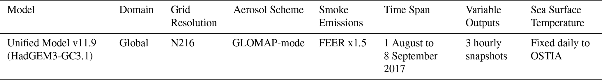
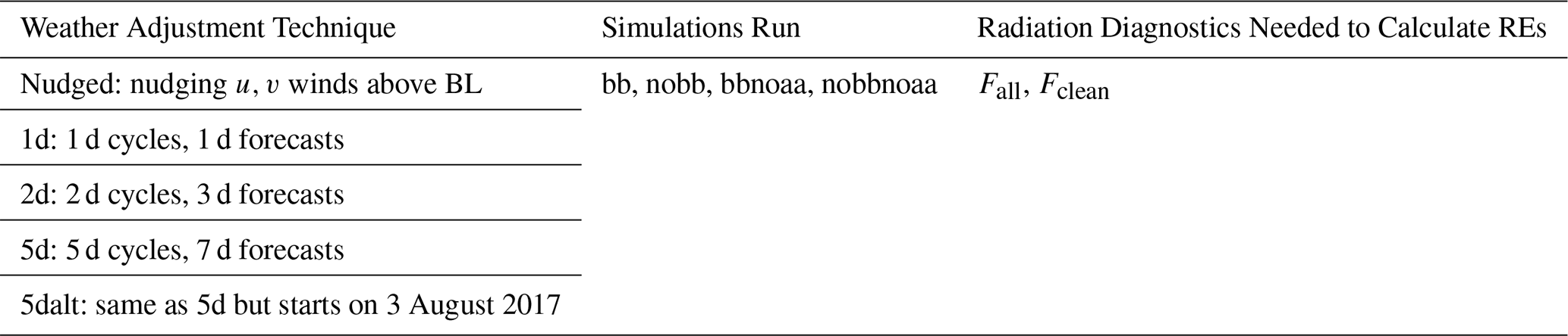
Table 2 Summary of the experimental setup. Each weather adjustment technique being tested is configured as in Table 1 and run four times: with smoke (bb), without smoke (nobb), with smoke but aerosol absorption turned off (bbnoaa), and without smoke where aerosol absorption is turned off (nobbnoaa). Each simulation uses the radiation scheme to save two diagnostics that calculate radiative flux at the top of Earth's atmosphere, F_all and F_clean. The all subscript indicates that extinction by all atmospheric constituents is included in the calculation. The clean subscript indicates that extinction by aerosols is ignored for the calculation. These diagnostics are then used to calculate REs according to the equations listed in Sect. 2.3.

The nudged simulations are initialized with the UM global operational meteorology on 1 August 2017 and thereafter nudged to the European Centre for Medium-Range Weather Forecasts (ECMWF) version 5 reanalysis, or ERA5 files, which provide fresh data every 6 h. Nudging is applied at each time step with a characteristic relaxation timescale (Telford et al., 2008) also set to 6 h. We follow the recommendations of Zhang et al. (2014) to nudge only horizontal (u,v) wind fields above 1920 m altitude, approximately corresponding to the height of the boundary layer (BL), with nudging strength ramping up to full over approximately 1 km (at around 3000 m altitude). There is no nudging of temperature anywhere and no nudging of winds below 1920 m altitude. We assume that this allows the model to simulate all temperature responses to aerosols and all cloud responses within the BL undisturbed. This nudged configuration closely follows the UM-UKCA simulation of Doherty et al. (2022), the UM simulation of Che et al. (2021), the UM simulation of Shinozuka et al. (2020), and the global UM simulation of Gordon et al. (2018). The only differences between our simulations and those listed above are that here we have updated the UM from previous versions to v11.9 and the organic carbon (OC) hygroscopicity value to 0.1, as described below (in Sect. 2.2), and we have used ERA5 instead of ERA-Interim as the reanalysis database for nudging (Hersbach et al., 2020).

The reinitialized simulations are initialized and reinitialized with the UM global operational meteorology at various frequencies. The reanalysis archives used for reinitializing (UM archives) and nudging (ERA5) are not an exact match. However, both are built on data assimilation, and our model evaluation in Sect. 3 suggests that they are comparable. We tested the following simulation setups, where the interval between reinitializations is always equal to the time period used in the analysis we present: 1 d long forecasts of which 1 d is used in the analysis (1d), 3 d long forecasts of which the last 2 d are used (2d), and two sets of 7 d long forecasts of which the last 5 d are used, one starting on 1 August 2017 (5d) and the other on 3 August 2017 (5dalt). For example, in the 5d setup, shown later in Fig. 4, the seven-day long forecasts start on 1 August, 6 August, and every 5 d until 5 September. Simulation results from the whole of the first forecast, the last 5 d of each subsequent forecast, and finally 7 and 8 September only from the last forecast are evaluated and used in our results. The overlap time, equal to the difference between the forecast length and the time period used for analysis, serves as the spin-up time to minimize discontinuity between reinitialized cycles (Pan et al., 1999; Gordon et al., 2023). The 2d set was chosen for comparable results to the simulations of Lu et al. (2018). The 5d set was chosen to match the configurations of the WRF-Chem simulations used by Doherty et al. (2022) and the WRF-CAM5 simulations used by Howes et al. (2023), Diamond et al. (2022), and Shinozuka et al. (2020). The 5dalt set was chosen to give insight into how sensitive the reinitialization method is to initial meteorological conditions when compared to the 5d set. The 1d set, which does not feature spin-up time between cycles, was chosen to test potential limitations of a high reinitialization frequency with respect to the timescales of cloud adjustments to smoke. Lastly, the free running set can also be thought of as a low reinitialization frequency test, where the forecast length chosen is the entire time span of the simulation.

2.2 Aerosol emissions and transport

All simulation sets represent aerosols using GLOMAP-mode, a two-moment modal aerosol microphysics scheme described in greater detail by Mann et al. (2010). GLOMAP-mode represents aerosols using five internally mixed, log-normal size modes: nucleation, Aitken soluble, Aitken insoluble, accumulation, and coarse. The aerosol scheme tracks sulfate, sea salt, black carbon (BC), and organic carbon (OC). Hygroscopicities of all substituents are based on Petters and Kreidenweis (2007), with the OC kappa value updated from 0.0 to 0.1 based on Fanourgakis et al. (2019) and Schmale et al. (2018). Dust is treated in a separate scheme with six size sections. The model assumes that OC is fully scattering and uses the GA7.1 updated complex refractive index for BC (Walters et al., 2019; Mulcahy et al., 2018). Sea salt, dimethyl sulfide, and dust emissions are all parameterized online. For all other emissions except BBA, standard CMIP6 inventories are used (Feng et al., 2020). Additionally, we use an offline oxidant chemistry scheme in which the required chemical oxidant fields (such as OH, O₃, HO₂ and H₂O₂) are provided as monthly mean climatologies derived from a simulation with online chemistry, as described in more detail by Walters et al. (2019). Further model details can be found in the description of the atmosphere and land components of HadGEM3-GC3.1 (Mulcahy et al., 2020).

The simulations that include smoke use biomass burning emissions from the Fire Energetics and Emissions Research (FEER) inventory, a MODIS satellite-based inventory (Ichoku and Ellison, 2014), following the recommendations of Pan et al. (2020). The inventory consists of BC and OC, at a daily time resolution and a 0.1° spatial resolution. BBA emissions are updated daily in the simulations and are initialized in the Aitken insoluble mode. The aerosol size distribution is used to derive CDNC via the activation parameterization of Abdul-Razzak and Ghan (2000). Both are passed to the radiation scheme to derive aerosol and cloud optical properties (Bellouin et al., 2013), where the radiation scheme can be used to compute both direct and cloud-mediated REs, as outlined in Sect. 2.3. Following the recommendations of Gordon et al. (2018), BBAs are injected throughout the BL such that concentrations are highest at the surface and taper down to zero at 3 km above the surface. The emitted smoke has an initial log-normal size distribution with an assumed mode centered at 120 nm diameter. We multiplied the FEER emissions by a factor of 1.5 for both BC and OC to obtain improved agreement between simulated and observed aerosol optical properties, as shown in Sect. 3. Emission scaling is a common practice among BBA model studies to improve agreement with observations and accounts, in part, for a known undercounting of the small fires that contribute most of the BBA emissions (Ramo et al., 2021; Pan et al., 2020; Reddington et al., 2016).

2.3 RE calculation formulas

We use the following formulations to disentangle and quantify component REs at TOA based on Ghan et al. (2012), Ghan (2013), and Gordon et al. (2018). The method involves four simulations (bb, nobb, bbnoaa, and nobbnoaa) and two calls to the radiation scheme in each simulation (F_all, F_clean). The simulations are with smoke (bb), without smoke (nobb), with smoke but aerosol absorption turned off (bbnoaa), and without smoke where aerosol absorption is turned off (nobbnoaa). We henceforth use this notation to reference simulations; thus, for example, we refer to the nudged simulation with smoke aerosol as Nudged_bb. All radiation scheme calls calculate net radiative flux (F) crossing the top of Earth's atmosphere. The all subscript indicates that extinction by all atmospheric constituents is included in the calculation. The clean subscript indicates that extinction by aerosols is ignored for the calculation. We apply the same equations for shortwave and longwave radiation, which is reasonable for REs over ocean in simulations with fixed sea surface temperature. This deviates from the recommendations of Ghan et al. (2012) to avoid aerosol-induced changes in surface albedo from contributing to the IRE; however, this should be negligible in the area we are examining.

$$\begin{array}{}\text{(1)}& {\displaystyle }\text{TRE}=(F_{\mathrm{all}}{)}_{\mathrm{bb}}-(F_{\mathrm{all}}{)}_{\mathrm{nobb}}\text{(2)}& {\displaystyle }\text{DRE}=(F_{\mathrm{all}}-F_{\mathrm{clean}}{)}_{\mathrm{bb}}-(F_{\mathrm{all}}-F_{\mathrm{clean}}{)}_{\mathrm{nobb}}\text{(3)}& {\displaystyle }\text{IRE}=(F_{\mathrm{clean}}{)}_{\mathrm{bbnoaa}}-(F_{\mathrm{clean}}{)}_{\mathrm{nobbnoaa}}\text{(4)}& {\displaystyle }\begin{array}{rl}\text{SDRE}& =\text{TRE}-\text{DRE}-\text{IRE}=\left[\right(F_{\mathrm{clean}}{)}_{\mathrm{bb}}-\left(F_{\mathrm{clean}}{)}_{\mathrm{nobb}}\right]\\ & -\left[\right(F_{\mathrm{clean}}{)}_{\mathrm{bbnoaa}}-\left(F_{\mathrm{clean}}{)}_{\mathrm{nobbnoaa}}\right]\end{array}\end{array}$$

Since the semi-direct effect mechanism for BBA is dominated by aerosol absorption, we assume that the use of simulations without aerosol absorption (noaa) allows us to isolate the cloud changes caused by just the IRE. The use of clean diagnostics removes the instantaneous DRE due to aerosol scattering, but the IRE may still include effects on clouds due to changes in temperature that result from aerosol scattering. We could have switched off scattering and absorption, in principle, as suggested by Ghan et al. (2012); however, we chose to follow Hansen et al. (1997) (and Gordon et al., 2018) in defining the semi-direct effect as the effect on clouds of absorption only. An advantage of this choice is that we can apply the same methodology to isolate the DRE due to scattering from the full DRE, as outlined below.

$$\begin{array}{}\text{(5)}& {\displaystyle }{\mathrm{\text{DRE}}}_{\mathrm{scattering}}=(F_{\mathrm{all}}-F_{\mathrm{clean}}{)}_{\mathrm{bbnoaa}}-(F_{\mathrm{all}}-F_{\mathrm{clean}}{)}_{\mathrm{nobbnoaa}}\text{(6)}& {\displaystyle }{\text{DRE}}_{\mathrm{absorption}}=\text{DRE}-{\text{DRE}}_{\mathrm{scattering}}\end{array}$$

Another advantage of our four simulation formulation is that it makes no assumptions about the background or non-BBA aerosols. By comparison, the formulation of Gordon et al. (2018) and Che et al. (2021), with only three simulations, uses nobb in place of our nobbnoaa simulation. This assumes that absorption by background aerosols, which include particles from anthropogenic fossil fuel burning, for example, is insignificant and is excluded from the calculation. Our findings suggest that absorption by the background aerosols is not large but should not be neglected. A disadvantage of both our formulation and the previous calculations of Gordon et al. (2018) and Che et al. (2021) is that cloud fields will not match between simulations with and without aerosol absorption (bb vs. bbnoaa, and nobb vs. nobbnoaa), so our calculated indirect effect neglects the effect of changes in cloud cover or thickness due to the semi-direct effect. The indirect effect also neglects the effect of aerosol absorption on the height of the aerosol layer, which we show in Sect. 4.7 affects the simulated CDNC. Equations (3) and (4), for IRE and SDRE, respectively, are therefore likely to be less accurate than the overall Cloud-mediated Radiative Effect (CRE), computed as

$$\begin{array}{}\text{(7)}& \text{CRE}=\text{IRE}+\text{SDRE}=(F_{\mathrm{clean}}{)}_{\mathrm{bb}}-(F_{\mathrm{clean}}{)}_{\mathrm{nobb}}\end{array}$$

This potential bias may also affect the decomposition of the complete DRE into an approximate DRE_scattering and DRE_absorbing by Eqs. (5) and (6), as this calculation also relies on the simulations with absorption switched off. We evaluate the total simulated smoke radiative effect (TRE), DRE, DRE_scattering, DRE_absorbing, IRE, and SDRE, using Eqs. (1)–(6) in Sect. 4.1–4.6. Section 4.7 further explores the consequences of using simulations without aerosol absorption in Eqs. (3)–(6) and presents CRE using Eq. (7).

3 Model evaluation

3.1 Observational datasets and evaluation strategy

We focus on August and early September 2017, the intersection of three field campaigns: NASA's ObseRvations of Aerosols above CLouds and their intEractionS (ORACLES), The UK's CLouds and Aerosol Radiative Impacts and Forcing (CLARIFY), and Atmospheric Radiation Measurement's (ARM's) Layered Atlantic Smoke Interactions with Clouds (LASIC). Barrett et al. (2022) show that the properties measured in these three campaigns generally agree well within uncertainties, giving confidence in the use of data from multiple platforms for model evaluations. In addition to data from these campaigns, we also use satellite retrievals from MODIS and Clouds and the Earth's Radiant Energy System (CERES). NASA's ORACLES campaign deployed flights from São Tomé to characterize smoke optical properties along the African coast and over the remote ocean. The UK's CLARIFY deployed flights out of Ascension Island to characterize smoke and cloud optical properties in the region where they mix together. ARM's LASIC mobile research facility was a surface campaign based out of Ascension Island, again focusing on the smoke–cloud mixing region. More detailed descriptions of the ORACLES, CLARIFY, and LASIC campaigns can be found in Redemann et al. (2021), Haywood et al. (2021), and Zuidema et al. (2018), respectively.

Spatial domains over which various smoke and cloud properties are evaluated were chosen to match those of Lu et al. (2018). The overall domain spans from +14 to −17° E and −17 to −2° N. A dividing line at 0° E divides the overall domain into two smaller domains, referred to as the coastal and remote domains, as depicted in Fig. 1. The following sections detail an evaluation of the model's performance for the Nudged_bb and 5d_bb simulations. Corresponding evaluations for Free Run_bb can be found in Figs. S2–S14 of the Supplement. Accurate quantification of BBA REs depends strongly on accurately simulating cloud properties, smoke optical properties, plume transport, and meteorology (Myhre et al., 2003). Our evaluation therefore focuses on these aspects.

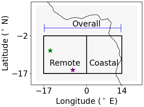
Figure 1 The spatial domain for model evaluation spans from +14 to −17° E and −17 to −2° N. A dividing line at 0° E splits the overall domain into the coastal and remote domains. The stars show the locations of Ascension Island (green) and St. Helena (purple).

3.2 Evaluating meteorology

Basic meteorology is evaluated through comparison to Vaisala radiosondes launched 3–4 times daily from Ascension Island during the LASIC campaign (Coulter et al., 1994) and the UK Met Office's radiosondes launched once daily from St. Helena in 2017. Model biases in temperature, relative humidity, or inversion height/strength are likely to significantly affect clouds, aerosol transport, and aerosol extinction. Linear interpolation was used to capture temperature and RH in the model at the location and time of each radiosonde. In Fig. 2, we show mean temperature and RH vertical profiles alongside corresponding model values of all the midday launches at both islands (approximately 12:00 UTC for Ascension Island and 11:15 UTC for St. Helena) and all the late night launches at Ascension Island (approximately 23:30 UTC). The profiles are divided into two time spans based on the date of the launch: 1 to 20 August and 21 August to 8 September. These time spans encapsulate meteorological changes in the free troposphere and the MBL, as shown in Fig. 2. These time spans coincide with changes in the ratio of above-cloud smoke to smoke within the MBL, as shown later in Fig. 6. The separation between major smoke periods that occurs on 20 August is also consistent with the strong free-tropospheric zonal winds that mark the beginning of austral spring, as seen in Table 2 of Ryoo et al. (2022). The individual launches that make up Fig. 2 occur from 15 through 31 August on Ascension Island and throughout the whole simulation time span, from 1 August through 8 September, on St. Helena. A sample of the individual radiosonde data and corresponding simulated profiles can be found in Fig. S1 of the Supplement.

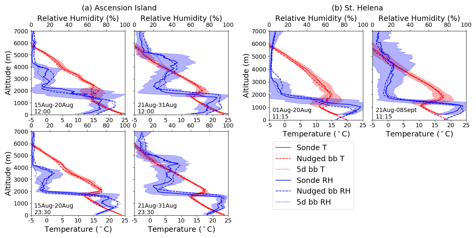
Figure 2 Mean vertical profiles of temperature (red) and RH (blue) from radiosondes launched during 1–20 August (left column) and 21 August–8 September (right column) at midday (top row) and midnight (bottom row) from (a) Ascension Island and (b) St. Helena. Corresponding Nudged_bb (dashed) and 5d_bb (dotted) simulated values are derived by linear interpolation to match the location and time of the radiosondes (solid). Standard deviation among the individual radiosondes that make up each grouping is shaded red for temperature and blue for RH. The date range and average launch time of the individual radiosondes that make up each grouping are shown in the bottom left.

The temperature profiles show a strong inversion, characteristic of stratocumulus cloud decks. On average, the Ascension Island inversion was recorded at a daytime/nighttime height of 1.9/1.7 km, respectively. This inversion height is generally captured well by the model, within 200/175 m and within 1.3/1.2 °C on average during the day/night, respectively, for Nudged_bb. The profiles at both islands show the frequent presence of two inversions, where the upper inversion marks the top of what was previously the continental BL over Africa. At St. Helena, an upper-level inversion with a strength of at least 1.0 °C was recorded by the radiosondes in 22 of 31 d in August 2017. On average, the lower St. Helena inversions are at 1.4 km altitude with a strength of 8.1 °C, and the upper inversions are at 2.8 km altitude with a strength of 2.3 °C. The model captures the lower inversion height well, within 220 m and within 1.6 °C for Nudged_bb. The upper inversion at St. Helena is represented by the simulation 60 % of the time. The strength of the upper inversion is 3–4 times weaker than the lower inversion. The model would likely capture the upper inversion better using a finer resolution. The performance of Nudged_bb is reasonably consistent with that of 5d_bb overall. The temperature profiles of both simulations are very similar, with both producing an inversion slightly below the observations on average. The 5d_bb simulation captured the height of the lower inversion at both locations slightly better than the Nudged_bb simulation, 50 m closer to observations on average. The upper inversion at St. Helena also appears to be closer to observations when it is represented, but the 5d_bb model only predicts 45 % of the inversions that were observed. Figures S2–S3 of the Supplement show the same evaluation for Free Run_bb, where average temperatures deviate from observations by up to around 3 K, highlighting the advantage of using a meteorological forcing technique.

RH profiles in the nudged and reinitialized models also match observations well, with mean absolute error within 8 % for Ascension Island and 10 % for St. Helena for both Nudged_bb and 5d_bb. We again see larger deviations, often of over 20 %, between the simulations with meteorological forcing techniques and that of Free Run_bb, as seen in Figs. S2 and S3. The performance of Nudged_bb is again reasonably consistent with that of 5d_bb overall, although the nudged simulation tends to have higher free-tropospheric RH compared to observations, while the 5d has lower free-tropospheric RH. Elevated water vapor signals of up to 60 % RH in the free troposphere in the SEA are often associated with smoke plumes (Pistone et al., 2021, 2019). This is therefore a likely signature of different wind fields impacting smoke advection and will likely affect (ambient) extinction coefficients, aerosol optical depth, and the DRE results between these simulations. For St. Helena, the increases in free-tropospheric RH correlate well with the height of the upper inversion. Some of the intricate details in observations at high altitudes are not captured in full by the model; however, they are generally captured. This is true of both the temperature and RH profiles. These findings are consistent with, and a slight improvement on, the radiosonde evaluation between Ascension Island and UM version 11.2, simulated from 1 to 10 August 2016, as seen in Fig. 5 of Gordon et al. (2018). However, the model biases are often still significant and may be responsible for some of the biases in simulated clouds and radiative fluxes we show next.

3.3 Evaluating clouds

We evaluate how well the models capture clouds using cloud liquid water path (LWP) and upwelling shortwave radiation at TOA (SWout). We use LWP from Collection 6.1 MODIS Level 3 daily cloud products from both Terra (MOD08) and Aqua (MYD08) satellites (Platnick et al., 2015). The MODIS L3 data aggregate cloud LWP values at the time of the satellites' passage on a 1° spatial resolution. Terra passes over the SEA domain around 10:30 UTC and Aqua around 13:30 UTC. In Fig. 3, we perform a basic comparison between MODIS and the simulations across the SEA, averaged over the whole simulation time period from 1 August to 8 September 2017. To prepare the comparison plot, we averaged all the outputs bounding the satellite overpass times, 09:00 and 12:00 UTC for Terra and 12:00 and 15:00 UTC for Aqua, across the whole simulation period.

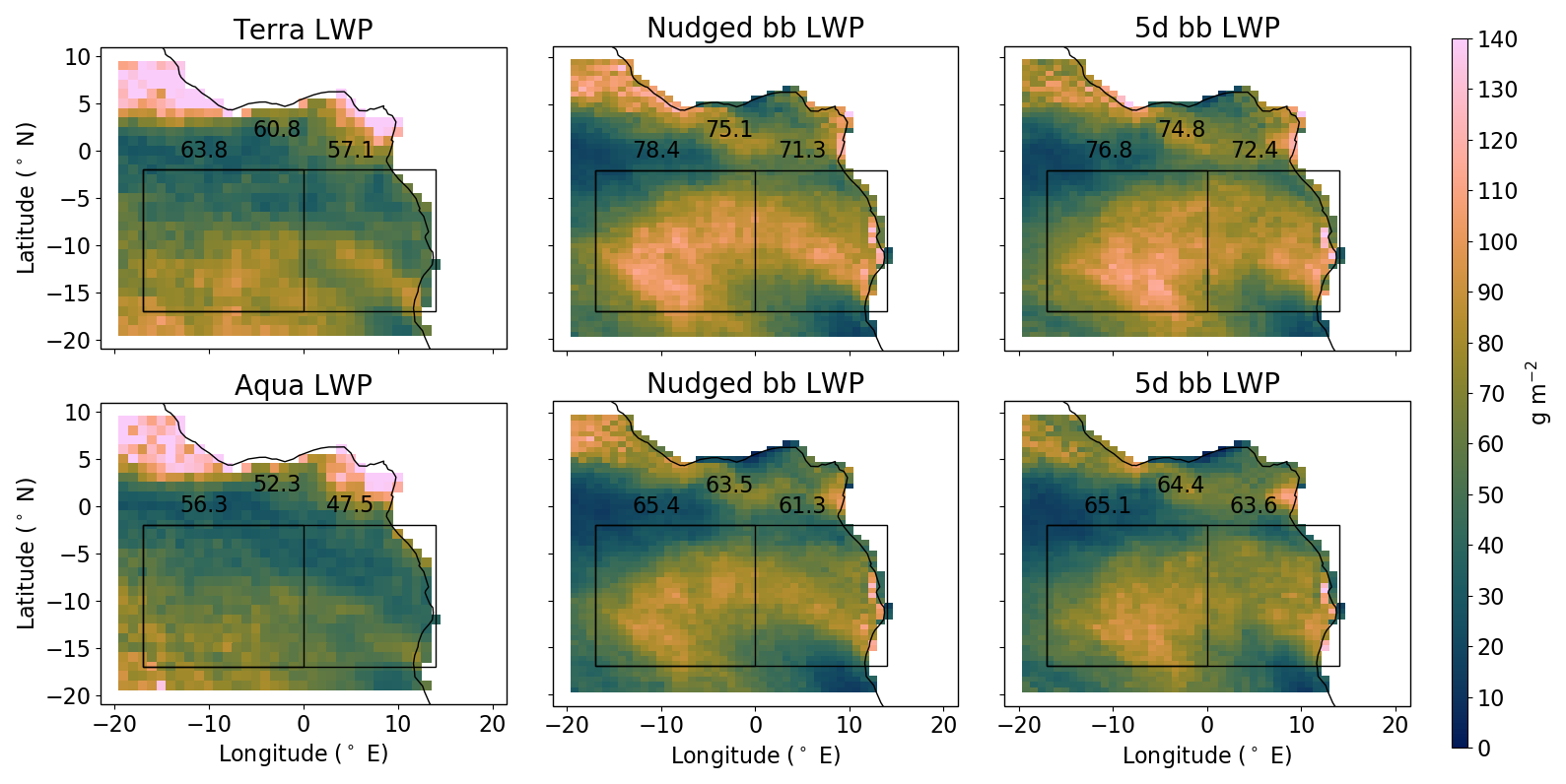
Figure 3 Mean LWP from 1 August to 8 September 2017 compared between MODIS, the Nudged_bb, and 5d_bb simulations for both Terra (top row) and Aqua (bottom row) satellites. Values are means at the time of the satellites' passing, approximately 10:30 UTC for Terra and 13:30 UTC for Aqua. Note that MODIS includes convective clouds between 0 and 10° N, which likely have large uncertainties in their LWP retrievals due to ice content. Clouds diagnosed from the model's convection parameterization are excluded from the model plots. Values printed are spatial averages of the overall (top), remote (left), and coastal (right) domains.

Overall, Nudged_bb and 5d_bb overestimate LWP in this region by approximately 20 %. Modeled LWP is particularly overestimated in the northern region of the coastal domain and southern region of the remote domain. To further quantify the performance, Fig. 4 shows a time series of simulated LWP in each domain compared to Terra; the corresponding evaluation for Aqua is shown in Fig. S6 of the Supplement. For Nudged_bb, with respect to Terra, we calculate a normalized mean bias (NMB) of +22 % in both the remote and coastal domains. For 5d_bb, we calculate a NMB of +20 % in the remote domain and +25 % in the coastal domain. The corresponding Free Run_bb results are shown in Figs. S4–S6 and show that biases are larger in this setup, as expected. Cloud LWP is consistently biased high by 25 %–50 %, much worse than the 20 %–25 % bias in our above forced simulations.

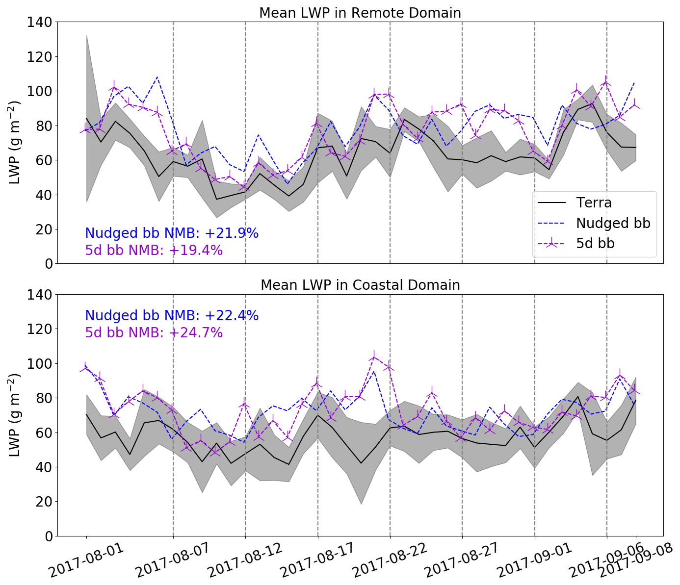
Figure 4 Time series of domain mean LWP as captured by Terra (black), the Nudged_bb (blue), and 5d_bb (purple) simulations for the remote (top) and coastal (bottom) domains. The vertical dashed lines show the transitions between forecasts of the 5d_bb simulation data used. For the 5d_bb simulation, each forecast is initialized two days prior to the transitions shown. Terra values are taken at approximately 10:30 UTC, with all data values less than zero removed. The gray shading shows the standard deviation around the L3 MODIS retrievals. Model values are taken at 10:30 UTC by linear interpolation between the 09:00 and 12:00 UTC outputs.

The Level 3 dataset provides an uncertainty estimate derived from pixel-level uncertainties of 8.7 g m⁻² for the overall domain or about 15 %. This estimate is in agreement with the 9.5 g m⁻² uncertainty estimate of Painemal et al. (2021). While our calculated LWP biases approach the uncertainty of the satellite retrieval, simulated LWP is likely still overestimated. Seethala and Horváth (2010) found MODIS tends to overestimate LWP for scenarios where aerosols lie above marine stratocumulus clouds, so the model's true biases may be even higher. A potential source of the overestimation is that the model MBL is not as decoupled in nature as the observed MBL, allowing more moisture to accumulate in the model MBL. Evidence of this can be seen in Fig. 2; however, it is more apparent in the individual radiosonde launches shown in Fig. S1 of the Supplement. Despite the overestimation, our results show a notable improvement in the model's skill at reproducing LWP in this region relative to the +66 % NMB of Gordon et al. (2018), who used UM version 11.2 with ERA-Interim nudging. The very high LWP bias of Gordon et al. (2018) corresponds to the factor of 4 high bias in cloud optical thickness (COT) of Doherty et al. (2022, their Fig. 24). An overestimation in COT is likely still present but now much less severe. The bias will impact our results for RE magnitudes by strengthening the CRE and biasing the DRE magnitude of partially absorbing aerosols high (toward more warming).

We compare modeled SWout to that measured by CERES on both Terra and Aqua satellites. SWout is an important measure of cloud albedo and is sensitive to cloud fraction (CF). We use CERES Level 3 SSF1deg-Hour Edition 4A for both Terra and Aqua to obtain CERES measurements. This dataset aggregates radiative fluxes at TOA hourly, at the location of the satellite's passing on a 1° spatial resolution (NASA, 2024a, b). In Fig. 5, we perform a basic comparison between CERES and the simulations across the SEA. To prepare the comparison plot, we regridded the model output to the slightly lower resolution of the CERES dataset. We also weighted the 3 hourly model outputs to match approximately the times of the CERES data. For example, a satellite swath recorded at 10:00 UTC was compared to a sum of model output at 09:00 weighted by $\mathrm{2}/\mathrm{3}$ and at 12:00 weighted by $\mathrm{1}/\mathrm{3}$. We show an average of all swaths compared over the full simulation time period from 1 August to 8 September 2017, in Fig. 5.

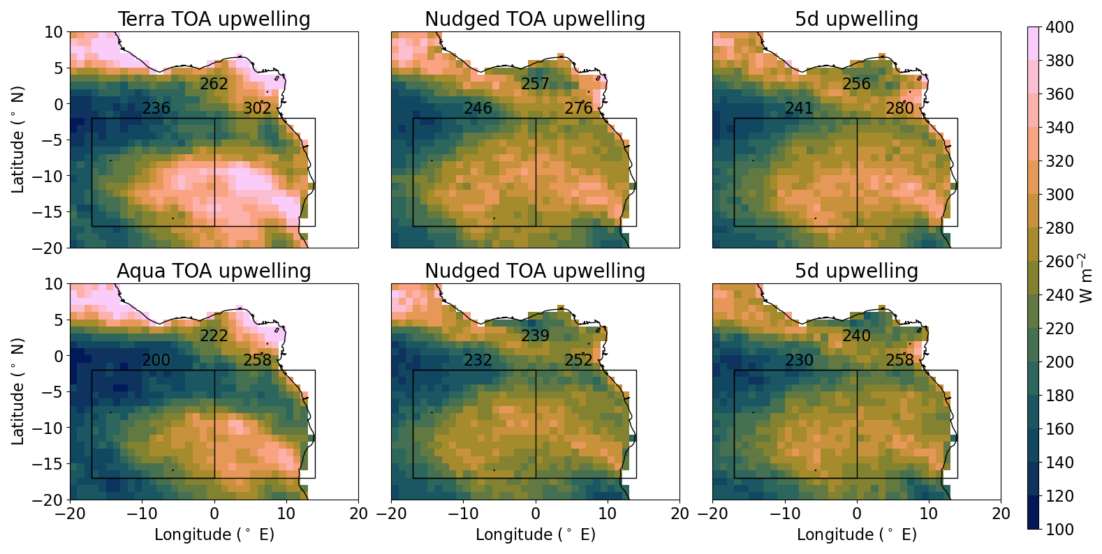
Figure 5 Mean SWout from 1 August to 8 September 2017 compared between CERES, Nudged_bb, and 5d_bb for both Terra (top row) and Aqua (bottom row) satellites. Values are the mean value at the time and location of the satellites' passing. The model was regridded to the lower resolution of the CERES dataset, masking out all locations outside the satellite swath and weighting the bounding model times to best match the satellite's overpass time. Values printed are spatial averages of the overall (top), remote (left), and coastal (right) domains.

The model slightly overestimates SWout in the remote domain by about 9 % and slightly underestimates it in the coastal domain by about 5 %. Overall, the model slightly overestimates SWout in this region by about 4 %. The Free Run evaluation is shown in Fig. S7, and time series of the domain averaged SWout for Nugded_bb, 5d_bb, and Free Run _bb are shown in Fig. S8 for Terra and in Fig. S9 for Aqua. These results again show a notable improvement in the model's skill relative to UM version 11.2 with ERA-Interim nudging, as seen in Fig. 15 of Gordon et al. (2018). Comparing the small 4 % overestimate in SWout to the more moderate 20 % overestimate in LWP, it seems likely that the model has a small, low bias in low-level cloud fraction (CF).

The retrieval dataset estimates a daily, regional uncertainty of 20 W m⁻² (Doelling et al., 2013). This was corroborated by Sicard (2019), who found that surface albedo differences between CERES and AERONET introduce an uncertainty of 15–20 W m⁻² in CERES radiative flux at TOA retrievals. Assuming that the uncertainty of the CERES L3 daily, regional retrieval is applicable to our simulations, a 20 W m⁻² uncertainty would account for all discrepancies in the overall domain for both satellites. The imperfect conversion of three hourly model diagnostics to compare against hourly satellite data may explain the larger biases in the individual domains that mostly cancel to give better agreement with observations in the overall domain. Considering this uncertainty, there is still a reasonably good match in the spatial patterns of outgoing SW radiation between the model and observations. While there may be compensating errors between CF and LWP, the relatively small biases in LWP together with the good simulation of SWout likely constrain the CF to be simulated reasonably well. This result aligns well with Mallet et al. (2021), who found the UM models CF well with respect to the Polarization and Anisotropy of Reflectances for Atmospheric Sciences coupled with Observations from a Lidar (PARASOL) and Cloud-Aerosol Lidar with Orthogonal Polarization (CALIOP) satellite retrievals when examining a larger domain over the SEA, most comparable to our overall domain. We interpret these results as an indication, albeit a tentative one, that clouds are sufficiently well simulated to yield reasonable RE calculations that will be representative of the August 2017 fire season if aerosols are also well simulated.

3.4 Evaluating smoke transport and optical properties

Smoke can be traced in our simulations through its black carbon content and therefore through its absorption coefficient. Figure 6 displays a time series of simulated absorption in the remote domain, showing smoke episodes moving westbound through the remote domain and reaching Ascension Island. In Fig. 6, as in Fig. 2, we can divide the time span into 1–20 August and 21 August–8 September, based on relative smoke amounts in the MBL and free troposphere. The first period has more smoke in the boundary layer and less in the free troposphere than the second. The MBL smoke in each time period is consistent with Zhang and Zuidema (2019, their Fig. 1). Nudged_bb (Fig. 6a) and 5d_bb (Fig. 6b) both capture the major smoke episodes well. Simulated absorption is qualitatively consistent with the smoke episodes measured during the CLARIFY and LASIC campaigns, both of which took place fully within our remote domain, as seen in Fig. 9 of Haywood et al. (2021) and Fig. 1 of Zhang and Zuidema (2019). A more in-depth comparison between simulated absorption and LASIC is shown later in Fig. 10. Figure 6 displays some differences in absorption coefficient between the Nudged_bb and 5d_bb simulations on a given day; however, in Fig. 7, we show BC concentrations average out to be approximately equal in both simulations over the two major smoke periods. Mean altitude values from 0 to 1 km and from 2 to 5 km are displayed to visualize smoke fully within and fully above the MBL. Figure 7a displays average concentrations within the first major smoke period from 1 to 20 August and Fig. 7b within the second major smoke period from 21 August to 8 September. Although slight, any differences in smoke will result in differences in calculated RE. Comparing the simulations, Nudged_bb on average has 2 % more smoke above the MBL and 8 % less smoke within the MBL than 5d_bb across the whole simulation period.

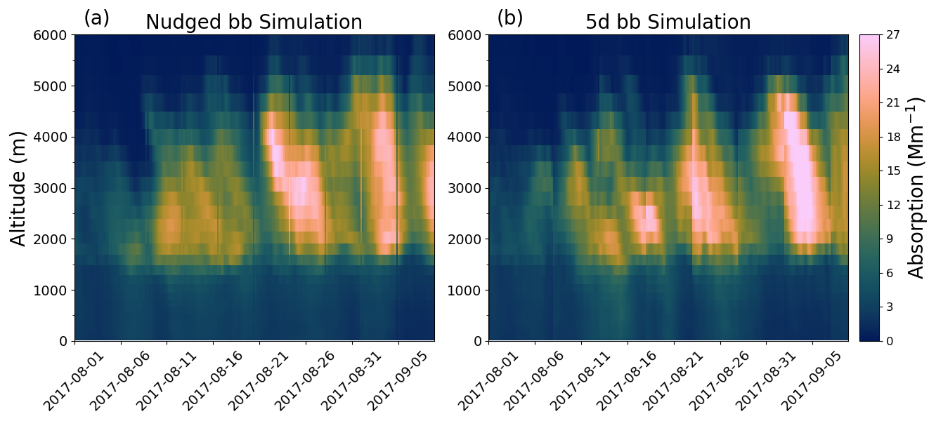
Figure 6 Time series of absorption coefficient averaged over the remote domain in the Nudged_bb (a) and 5d_bb (b) simulations. Smoke episodes are divided into two major time periods: 1–20 August and 21 August–8 September.

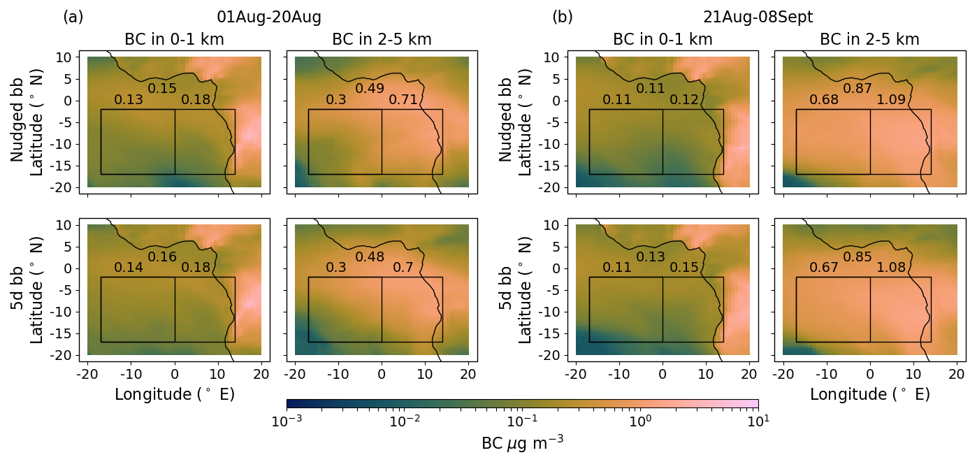
Figure 7 BC mass concentrations for both the Nudged_bb (top row) and 5d_bb (bottom row) simulations averaged over 1–20 August (a) and 21 August–8 September (b) 2017. Mass concentrations are averaged from 0 to 1 km (left column) and from 2 to 5 km (right column) to show within and above the MBL, respectively. Values printed are spatial averages of the overall (top), remote (left), and coastal (right) domains.

To examine biases in smoke amount compared to observations, we compare simulated absorption coefficient, extinction coefficient, BC mass concentration, and OA mass concentrations to the corresponding measurements from the ORACLES 2017, CLARIFY 2017, and LASIC field campaigns. The ORACLES and CLARIFY flight data are represented by 1 min averages, excluding in-cloud data. An interpolation algorithm was then used to match UM grid locations with the flight data. The final plots were made by averaging the interpolated data every 150 m to reduce the noise. The analysis is divided by flight and domain, producing a vertical profile of each variable for ORACLES in the coastal domain, ORACLES in the remote domain, and CLARIFY in the remote domain. The LASIC ground campaign data from the Department of Energy Atmospheric Radiation Measurement (ARM) Mobile Facility 1 were recorded on a hillside at around 350 m above sea level and are represented in a time series using three hourly averages. UM data were extracted at the same location as the LASIC mobile facility, where data are outputs from the model at a three hourly resolution (Sect. 2.1).

The UM derives extinction, absorption, and scattering coefficients at many wavelengths of light; however, we chose 550 nm at standard temperature and pressure (STP) conditions, 1013.25 hPa and 273.15 K, for this analysis as it most closely matches the observations. On the NASA P-3 aircraft during ORACLES, the absorption coefficient was measured in situ at STP with a particle soot absorption photometer (PSAP) at 470, 530, and 660 nm wavelengths, corrected following Virkkula (2010). Scattering coefficient was measured in situ at STP with a nephelometer at 450, 550, and 700 nm wavelengths, corrected following Anderson and Ogren (1998). To obtain the absorption coefficient at 550 nm, STP, we calculated an absorption Ångström exponent offline using the measurements provided and then used this to calculate the absorption coefficient at 550 nm wavelength (equations are given, for example, as per Eqs. 8–9 of Perim de Faria et al., 2021). Finally, extinction coefficient at 550 nm, STP, was calculated by summing the absorption and scattering coefficients. On the FAAM BAe-146 during CLARIFY, absorption coefficient was measured in situ at STP by the EXCALABAR photo-acoustic spectrometer (PAS) at 405, 515, and 660 nm wavelengths. Extinction coefficient was measured in situ at STP by the EXCALABAR cavity ring-down spectrometer (CRDS) at 405 and 660 nm wavelengths. The same equations were used again to calculate an Ångström exponent and corresponding values for both absorption and extinction coefficient measurements at 550 nm, STP. Both flights measured dry aerosol properties, while the UM can output both dry and ambient RH values. The resulting absorption and extinction coefficient vertical profiles are shown in panels (a), (b), and (c) of Figs. 8 and 9, respectively. During LASIC, absorption was measured in situ using a PSAP at 529 and 648 nm wavelengths, corrected using an average of the Virkkula (2010) and Ogren (2010) corrections. Scattering was measured in situ using a nephelometer at 550 nm wavelength. We again calculated an Ångström exponent and a corresponding value for absorption coefficient at 550 nm. Extinction coefficient at 550 nm, STP, was calculated offline by summing the 550 nm absorption and scattering coefficients. These LASIC measurements were performed with some drying; RH was estimated to be below 25 % for absorption and approximately 45 %–60 % for scattering (Barrett et al., 2022). Although not completely dry (RH < 40 %), the results of Dedrick et al. (2022) indicate that dry model diagnostics are a closer comparison to the LASIC measurements than ambient model diagnostics. Additionally, absorption and extinction measurements for aerosols larger than 1.0 µm are excluded from the LASIC data since BBAs are less than 1.0 µm, as shown in Dobracki et al. (2023) (their Fig. 3). The resulting time series are shown in panels (a) and (b) of Fig. 10.

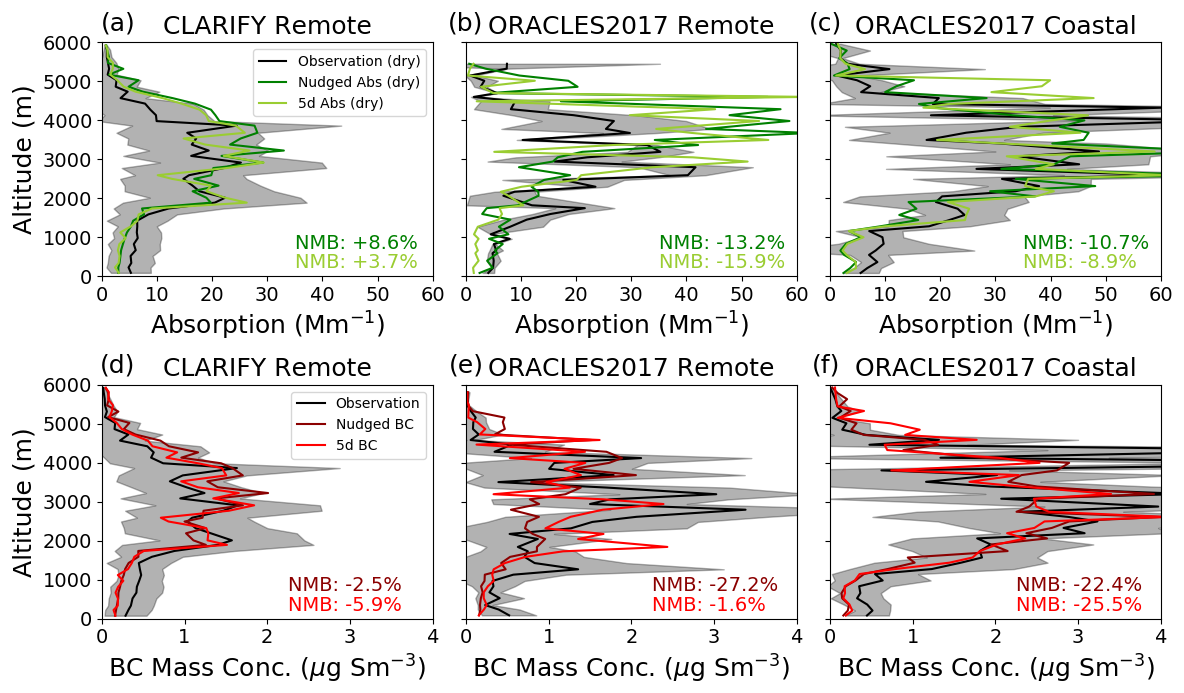
Figure 8 Absorption coefficient (green) and BC mass concentration (red) compared between Nudged_bb (darker), 5d_bb (lighter), and flight data (black) for the ORACLES2017 flights in the coastal domain (c, f), ORACLES2017 flights in the remote domain (b, e), and CLARIFY flights in the remote domain (a, d). All variables are compared at STP (1013.25 hPa, 273.15 K) and, in the case of absorption, at 550 nm wavelength. The flight data are represented by 1 min means omitting in-cloud data. Corresponding model values were captured using an interpolation algorithm to match UM grid locations to the flight path. The final plots were produced using 150 m averages to reduce noise. The standard deviation within these 150 m intervals for the flight data is shaded gray.

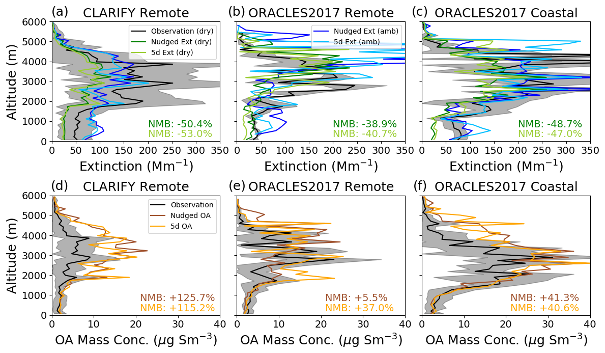
Figure 9 Extinction coefficient (green for dry, blue for ambient RH) and OA mass concentration (orange) compared between Nudged_bb (darker), 5d_bb (lighter), and flight data (black) for the ORACLES2017 flights in the coastal domain (c, f), ORACLES2017 flights in the remote domain (b, e), and CLARIFY flights in the remote domain (a, d). All variables are compared at STP (1013.25 hPa, 273.15 K) and, in the case of extinction, at 550 nm wavelength. The flight data are represented by 1 min means omitting in-cloud data. Corresponding model values were captured using an interpolation algorithm to match UM grid locations to the flight path. The final plots were produced using 150 m averages to reduce noise. The standard deviation within these 150 m intervals for the flight data is shaded gray.

On the NASA P-3, refractory BC mass concentration was measured using a single particle soot photometer (SP2) at the instrument chamber's temperature and pressure, and non-refractory OA mass concentration was measured using an aerosol mass spectrometer (AMS) at STP. On the FAAM BAe-146, refractory BC mass concentration was measured using a SP2 at STP, and OA mass concentration was measured using an AMS at STP. For consistency, we converted the ORACLES BC concentrations from chamber to standard temperature and pressure, so all concentrations shown are in micrograms per standard cubic meter (µg Sm⁻³). The resulting BC and OA mass concentration vertical profiles are shown in panels (d), (e), and (f) of Figs. 8 and 9, respectively. During LASIC, refractory BC mass concentration was measured using a SP2, and non-refractory OA mass concentration using an Aerosol Chemical Speciation Monitor (ACSM), both at STP. The resulting time series are shown in panels (c) and (d) of Fig. 10.

Across all variables, the locations of peak values measured relative to the modeled peaks are an indicator of how well the model captured vertical smoke transport throughout the SEA. The amount of smoke transported is best compared through the NMB of each variable, which can be found printed in each subfigure. Each variable is discussed in more detail below, but in general, the positions of peak values align well between measurements and simulations. We conclude from Figs. 6–10 that the model generally captures smoke transport well in the SEA, and the Nudged_bb and 5d_bb simulations mostly align well with each other.

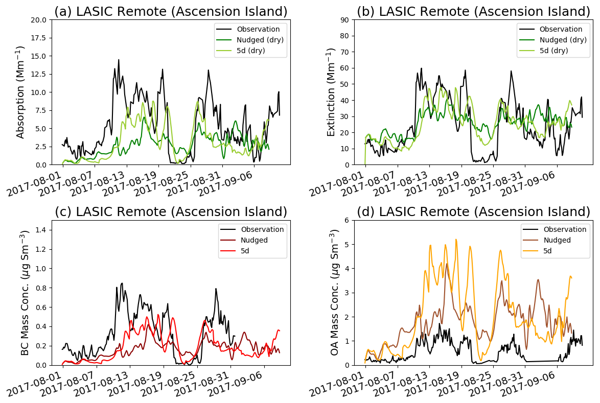
Figure 10 Absorption coefficient (a, green), extinction coefficient (b, green), BC mass concentration (c, red), and OA mass concentration (d, orange) compared between the Nudged_bb (darker), 5d_bb (lighter), and near surface Ascension Island measurements from LASIC (black). All variables are compared at STP (1013.25 hPa, 273.15 K) and, in the case of absorption and extinction, at 550 nm wavelength. LASIC data are represented by three hourly means, with aerosols larger than 1.0 µm excluded from the absorption and extinction measurements. Model data are extracted at the location of the ARM Mobile Facility 1 of LASIC at a three hourly resolution. LASIC measurements were performed with some drying, and although not perfectly dry (RH < 40 %), dry model diagnostics are used as they are the closest comparison.

The absorption coefficient shows good agreement in the coastal domain in Fig. 8, with an overall NMB within 10 % of observations. This small absorption low bias in the coastal domain stays relatively consistent downwind in the remote domain. A similar slightly low bias can be seen in the boundary layer throughout Fig. 8 and in the near-surface values of Fig. 10 at Ascension Island, a far west (downwind) location within the remote domain (see Fig. 1). In both domains, we again see higher absorption above the MBL for 5d_bb than for Nudged_bb, corroborating our conclusion from Fig. 7. We calculate an overall domain NMB for all flight data and the model's corresponding dry absorption values of 0.2 % for Nudged_bb and −2 % for 5d_bb. Our results are consistent with, and show a slight improvement upon, the small low-biased absorption results of previous studies with similar UM configurations, such as Doherty et al. (2022) and Shinozuka et al. (2020). The absorption coefficient should correlate well with BC mass concentration, and we do see this in comparing Fig. 8a to d, Fig. 8b to e, and Fig. 8c to f. The observations show a decrease in both absorption coefficient and BC mass concentration as the smoke travels from its source to the coastal and later remote domain. Our simulations generally follow these trends well. For BC mass concentration, we calculate an overall domain NMB of −16 % for Nudged_bb and −15 % for 5d_bb. The low BC bias is also consistent with the findings of previous UM evaluations such as Doherty et al. (2022), Shinozuka et al. (2020), and Das et al. (2017). These same biases (low for both absorption and BC) can be seen at Ascension Island in Fig. 10, suggesting that smoke in the boundary layer is slightly underestimated by the model.

The extinction coefficient is in poorer agreement with observations compared to the absorption coefficient in all the domains of Fig. 9. The measurements are taken dry; however, many previous studies evaluate against ambient extinction values due to the absence of dry model diagnostics. The UM can write out both dry and ambient optical properties, so we include both in our analysis. We calculate an overall domain NMB for dry extinction of −50 % for both Nudged_bb and 5d_bb. We find ambient RH model values closer to observation for all the extinction plots, with an overall domain NMB of −10 % for Nudged_bb and −11 % for 5d_bb. The extinction coefficient should correlate well with OA mass concentration. We do see good correlation; however, OA mass concentration is biased high, while extinction is biased low. This inconsistency was also found by Doherty et al. (2022) and Shinozuka et al. (2020). The CLARIFY BAe-146 measured supermicron aerosols, while the ORACLES P3 did not. Barrett et al. (2022) showed that the supermicron aerosols, which are absent in our model, make a contribution; however, it is not substantial enough to explain the model bias we observe. Biases in species other than BC and OA, for example, nitrate, which is not included in our model, are also unable to fully explain the extinction bias we observe. The high bias in OA (which has no substantial corresponding bias in aircraft-measured BC) is in part caused by the absence of chemical processes that reduce OA as smoke plumes age in our simulations (Dobracki et al., 2023; Sedlacek et al., 2022). This could explain why the high bias in OA worsens between ORACLES coastal and CLARIFY remote as the smoke plume ages. The observations show a decrease in extinction coefficient and OA mass concentration as smoke transits the SEA from east to west, and the simulations generally follow these trends well despite the biases presented. These same biases (low for extinction, high for OA) can also be seen at Ascension Island in Fig. 10.

Overall, our evaluation suggests that absorption and BC are represented generally well within the simulations, while extinction is biased low and OA is biased high. All four variables suggest that smoke burden and transport are represented well within our simulations, and the most likely source of the extinction/OA bias stems from an underrepresentation of BBA scattering efficiency (Doherty et al., 2022). Above cloud BBA scattering should, in theory, have minimal impacts on BBA REs because BBA absorption dominates the DRE and SDRE mechanisms, and any radiation that would be scattered by the smoke would instead be scattered by the cloud. However, DRE cooling due to smoke above cloud-free ocean surface would be impacted and biased to lower magnitudes by a low bias in BBA scattering. Since the REs are calculated over a region that contains a mix of cloudy and cloud-free ocean, our smoke evaluation suggests that DRE and TRE will be likely biased high overall (too positive). Corresponding smoke evaluations for Free Run_bb are shown in Figs. S10–S14. Again, we see the same biases exist in this setup, but they are substantially more pronounced. For example, aerosol absorption is underestimated by 10 %–30 % and extinction by 40 %–65 %. These larger biases affect REs, as we show in the next section, and motivate the constraints of reanalysis meteorology in the other simulations. Overall, our evaluation suggests we have made substantial improvements to some aspects of the model (mainly clouds) compared to previous studies (Doherty et al., 2022; Shinozuka et al., 2020; Gordon et al., 2018); however our RE results may still be affected by the remaining biases in our simulations.

4 Radiative effects

The REs are calculated over the domains shown in Fig. 1. For all domains, only REs over the ocean at TOA were calculated. The time spans we averaged over to produce RE magnitudes are the whole simulation period from 1 August to 8 September 2017 and the two significant time spans shown previously in Figs. 2 and 6: 1 to 20 August and 21 August to 8 September.

4.1 Total radiative effects

Figures 11 and 12 summarize grid resolved TRE calculated over ocean at TOA, according to Eq. (1), for each weather adjustment technique across the various domains and time spans. The full list of resulting magnitudes from all simulations, across each division of domain and time, is shown in Table 3.

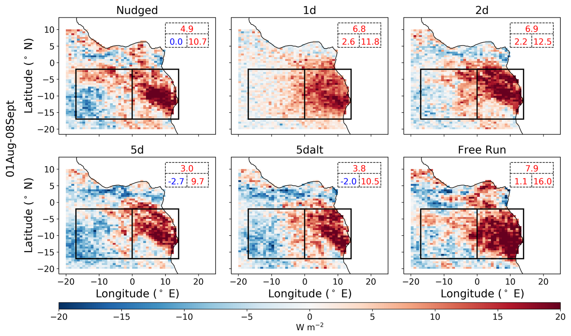
Figure 11 TRE calculated according to Eq. (1) across all simulation sets and averaged over the SEA from 1 August to 8 September 2017. Values in the top right corner represent spatial averages of the overall (top), remote (left), and coastal (right) domains. Positive mean magnitudes are shown in red for warming, and negative mean magnitudes are shown in blue for cooling.

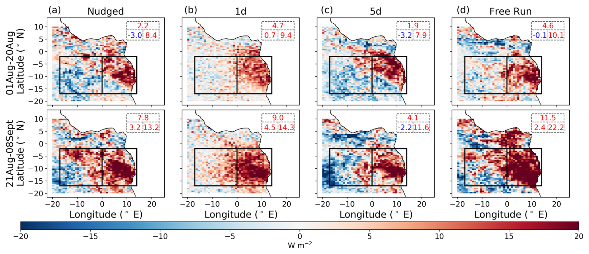
Figure 12 TRE calculated according to Eq. (1) and averaged over the SEA from 1 to 20 August (top row) and 21 August to 8 September (bottom row) 2017 for the Nudged (a), 1d (b), 5d (c), and Free Run (d) simulation sets. Values in the top right corner represent spatial averages of the overall (top), remote (left), and coastal (right) domains. Positive mean magnitudes are shown in red for warming, and negative mean magnitudes are shown in blue for cooling.

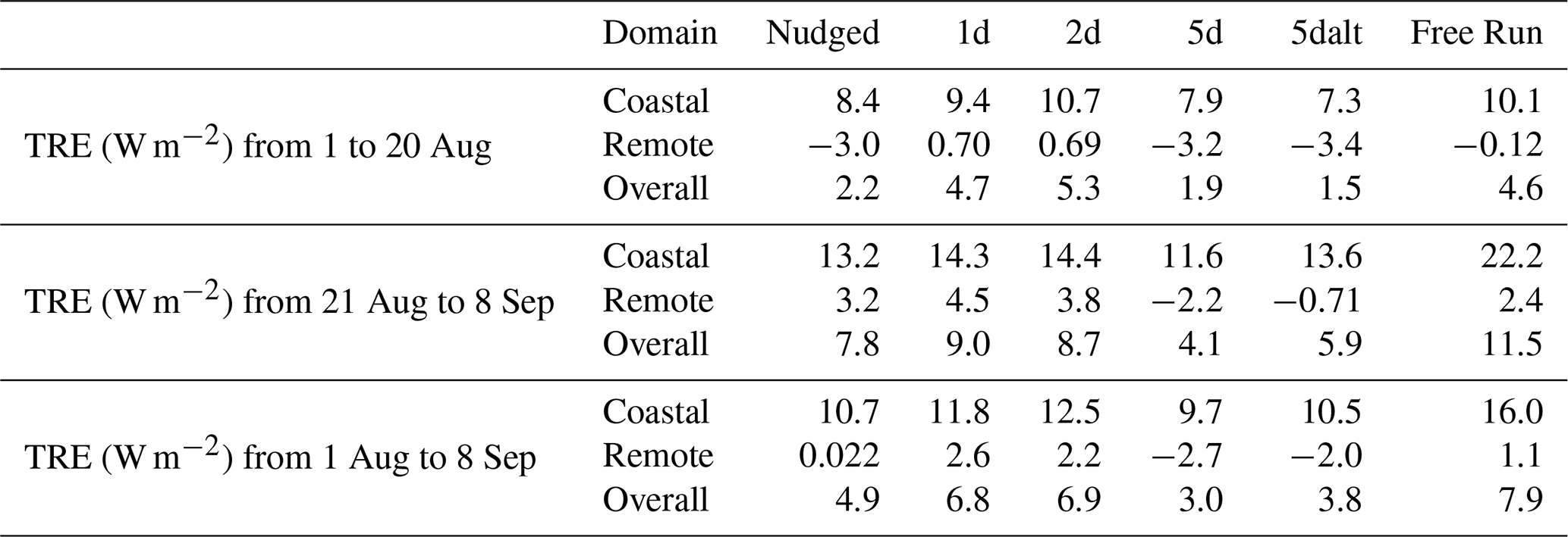
Table 3 TRE (W m⁻²) averaged over each domain from 1 to 20 August, 21 August to 8 September, and 1 August to 8 September 2017.

Each weather adjustment technique displays the same general trend of warming in the overall domain by 3.0–7.9 W m⁻², with the strongest warming effects in the coastal domain. There is a mix of warming and cooling effects in the remote domain that vary between the different techniques; however, there is agreement that the remote domain effects are weaker in comparison to the warming effect of the coastal domain. The deviations in magnitude, and for the remote domain, deviations in sign, between weather adjustment techniques are explored further in the upcoming sections discussing the component RE results that make up the TRE.

4.2 Direct radiative effects

Figure 13 shows the grid resolved Nudged DRE calculated over the ocean at TOA, according to Eq. (2). Nudged DRE is qualitatively representative of all the simulations. The full list of DRE magnitudes from all simulations, across each domain and time span, is shown in Table 4.

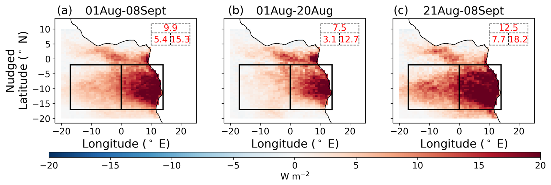
Figure 13 Nudged DRE calculated according to Eq. (2) and averaged over the SEA for 1 August–8 September (a), 1–20 August (b), and 21 August–8 September (c) 2017. Values in the top right corner represent spatial averages of the overall (top), remote (left), and coastal (right) domains. Positive mean magnitudes are shown in red for warming, and negative mean magnitudes are shown in blue for cooling.

Table 4 DRE (W m⁻²) averaged over each domain for 1–20 August, 21 August–8 September, and 1 August–8 September 2017.

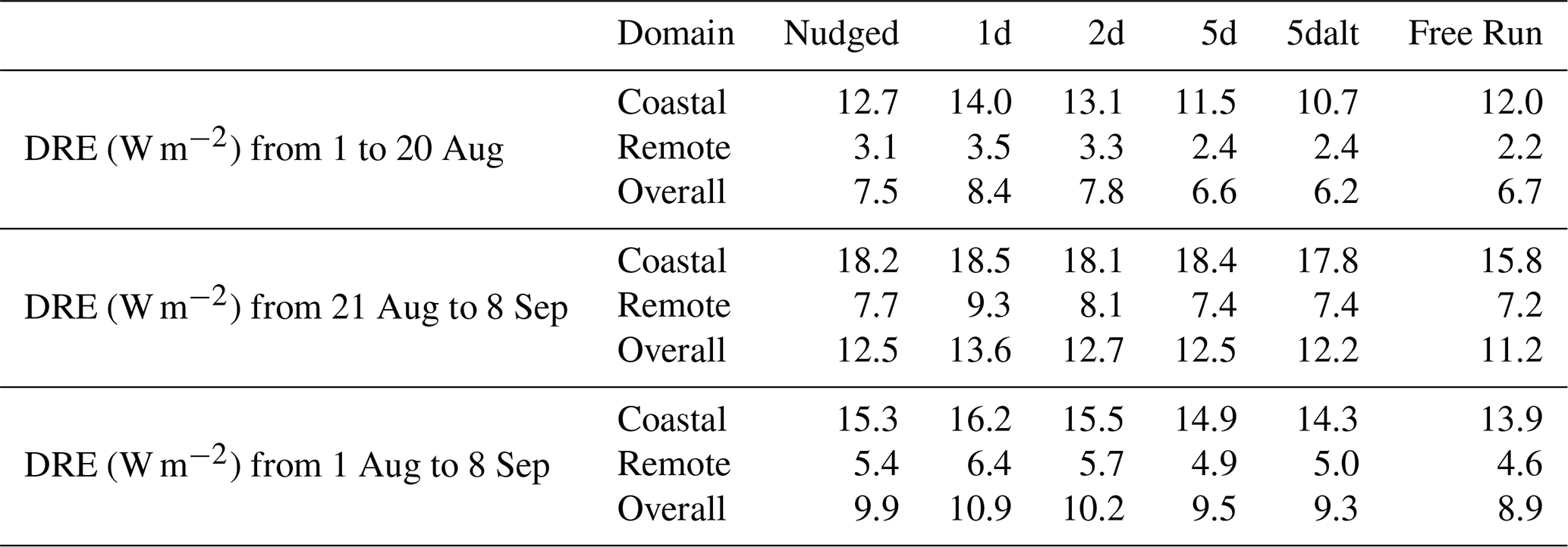
Simulations with all weather adjustment techniques agree that the DRE is strongly warming. The strongest warming occurs near the coast and the effect weakens moving westward over the remote ocean. The magnitudes of the DRE are consistently largest in 1d and decrease as the interval between reinitializations increases in length, with the smallest magnitudes usually coming from Free Run. The Free Run simulations can be thought of as using a forecast length that matches the simulation time span. The Nudged magnitudes consistently fall between that of 2d and 5d. Figure 13 also depicts regions of weak cooling. The locations where this occurs correlates with locations where smoke is above ocean instead of the cloud (Fig. 3), where the magnitude of cooling is indicative of the smoke amount transported to these remote ocean regions. Lastly, each technique agrees that the effects from 21 August to 8 September are stronger than those from 1 to 20 August. This stems from a greater amount of smoke present in the second time period relative to the first (Fig. 6).

Our DRE results are broadly consistent with previous studies. Our results are most easily compared to Che et al. (2021) who also found strong DRE warming near the coast, a weakening of warming effects moving westward, and a weakly cooling effect far west over the remote ocean. Che et al. (2021) used the same model and a configuration comparable to our Nudged set, with notable differences being their use of a coarser grid resolution, ERA-Interim as the nudging database, and GFAS for fire emissions. These differences aside, the model biases in their model are relatively similar to ours. They calculate a DRE of +7.5 W m⁻² for a cloudy region of the SEA averaged over July–August of 2016 and 2017 (their Fig. 9). This result is most comparable to the +9.9 W m⁻² results of our Nudged DRE for the overall domain from 1 August to 8 September. Different choices in temporal and spatial averaging may partly account for our larger result. Redemann et al. (2021) report more aerosol extinction measured in ORACLES 2017 compared to ORACLES 2016 (their Fig. 13), and our overall domain does not extend as far west as the cloudy region of Che et al. (2021), therefore resulting in a lower contribution from the weakly cooling DRE in the region of the stratocumulus-to-cumulus transition in our result. Doherty et al. (2022) noted that DRE is most sensitive to aerosol optical depth (AOD), COT, and CF. In our model evaluation, with extinction coefficient representative of AOD (Fig. 9), LWP of COT (Fig. 4), and SWout of CF (Fig. 5), we find simulated AOD biased low, COT biased slightly high, and CF well modeled. Both the AOD bias, leading to an underestimation of DRE cooling, and the COT bias, leading to a slight overestimation of cloud albedo, may lead to DRE magnitudes that are higher in our simulations than the real DRE.

A high bias in positive DRE in the UM is also a conclusion of Doherty et al. (2022). They calculated DRE using average aerosol and cloud properties from both the UM and from various measured satellite sources. For example, they found a mean DRE of +20.7 W m⁻² for the UM and +16.3 W m⁻² in observations in one 2×2° region (their “meridional 2, grid box 5”) averaged over 9 August to 2 September 2017 (their Table 3). Further north, they found a much larger discrepancy between the UM's (still positive) DRE and observations by a factor of 7.3, likely due to a high-biased cloud fraction combined with a high-biased COT in the UM simulations for that paper. Meridional 2, grid box 5 is a cloudy area within our coastal box, making our most comparable result the +15.3 W m⁻² of our Nudged DRE in the coastal box from 1 August to 8 September. However, this comparison is not perfect, as here we present a mean of instantaneous DRE values, while Doherty et al. (2022) present an instantaneous DRE calculated using mean values.

Although the biases in LWP and extinction and the results of Doherty et al. (2022) led us to believe that our DRE results are likely biased high, our results are likely realistic. de Graaf et al. (2019) calculated DRE purely from the OMI and MODIS measurements of NASA's Aura and Aqua satellites, respectively. They found an above-cloud DRE of +25 W m⁻² for the SEA during the 2006 fire season and further showed that this value was likely larger for the 2017 fire season (their Fig. 9a). Their result is most comparable to our result in the overall domain using only time averaged values from 13:30 UTC, the approximate time of Aura and Aqua's SEA overpass. Using only 13:30 UTC time points, we calculate a DRE within the overall domain over 1 August to 8 September of +20 to +25 W m⁻² across all weather adjustment techniques (without removing areas of clear sky).

4.3 DRE scattering and absorption

Using Eqs. (5) and (6), we separate the full DRE into its scattering and absorbing components. Figure 14 shows the scattering and absorption components of the Nudged DRE shown in Fig. 13. The full list of DRE_scattering and DRE_absorbing magnitudes from all simulations, across every domain and time span, is provided in Tables S1 and S2 of the Supplement.

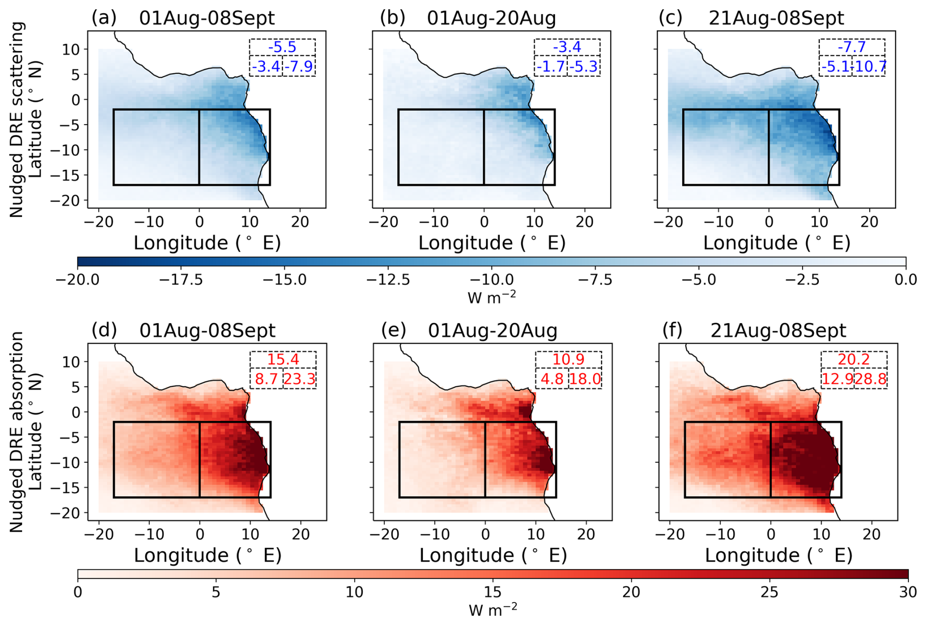
Figure 14 Nudged DRE from Fig. 13 separated into scattering (a–c) and absorption (d–f) components according to Eqs. (5) and (6). Values in the top right corner represent spatial averages of the overall (top), remote (left), and coastal (right) domains. Positive mean magnitudes are shown in red for warming, and negative mean magnitudes are shown in blue for cooling.

The overall sign of the DRE is dependent on the albedo of the scene beneath the smoke (Chand et al., 2009). We can expect to see both heating and cooling at the same grid locations; however, BBA scattering is more impactful over clear ocean, and BBA absorption is more impactful over clouds. Both DRE scattering and absorption are strongest along the coast near the smoke's source. The scattering RE is slightly more important relative to the absorption RE in the remote box than in the coastal box, as expected, since the scene albedo (Fig. 5) in the remote box is lower than that in the coastal box.

4.4 Indirect radiative effects

Figure 15 shows the grid resolved Nudged IRE calculated over the ocean at TOA, according to Eq. (3). Following this equation, we do not consider the impact of aerosol absorption on smoke layer height and the change to CDNC that results, but this is discussed in Sect. 4.7. Nudged IRE is qualitatively representative of the IRE findings for all the simulations. The full list of resulting magnitudes from all simulations, across every domain and time span, is shown in Table 5. All techniques calculated a more negative IRE magnitude from 21 August to 8 September, relative to 1 to 20 August. This result is expected, as more smoke is present in the latter time period (Fig. 6).

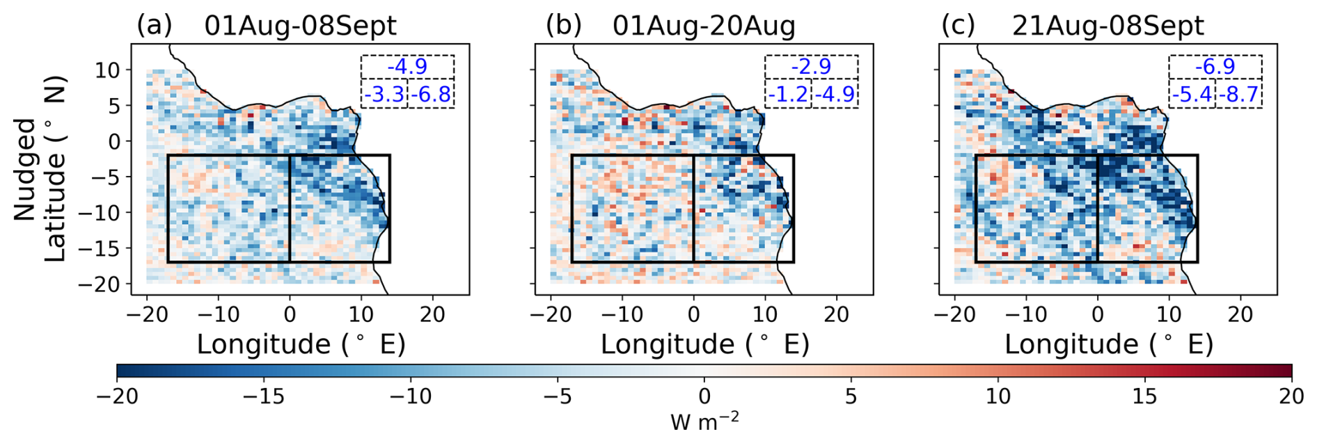
Figure 15 Nudged IRE calculated according to Eq. (3) and averaged over the SEA for 1 August–8 September (a), 1–20 August (b), and 21 August–8 September (c) 2017. Values in the top right corner represent spatial averages of the overall (top), remote (left), and coastal (right) domains. Positive mean magnitudes are shown in red for warming, and negative mean magnitudes are shown in blue for cooling.

IRE should correlate with changes in CDNC, LWP, and CF between the bbnoaa and nobbnoaa simulations, following Eq. (3). In Fig. S15, we show this comparison between the Nudged IRE and the changes in LWP, CF, and CDNC across the Nudged_bbnoaa and Nudged_nobbnoaa simulations. CF changes by up to around 6 %, while the 10 g m⁻² change in LWP in the domains corresponds to a change of around 15 % (Fig. 4). It appears from Fig. S15 that the Twomey effect, from changes in CDNC and adjustments to LWP, must be a stronger driver than adjustments to CF for the IRE. While smoke mostly acts through the indirect effect to increase LWP, it sometimes also seems to decrease CF. While the IRE is overall negative, Fig. 15 shows a slight warming in some areas. These changes are related to changes in the locations of clouds and boundary layer heights between simulations, rather than to changes in CDNC.

In Free Run, there is an accumulating departure in simulated clouds between simulations with and without smoke that produces a positive IRE in the remote domain from 1 to 20 August. In addition, the cooling effect produced in Free Run in the overall domain in the second time period is 1 order of magnitude larger than that in the first. These results can be seen in Table 5 but are made more apparent in Fig. S16 of the Supplement, in which we show the spatial variability of the IRE over each time period. The drastically different magnitudes between the first and second time period, and also the large indirect warming from smoke in some other parts of the domain, suggest that the Free Run technique is not well suited to quantifying REs over such short time periods.

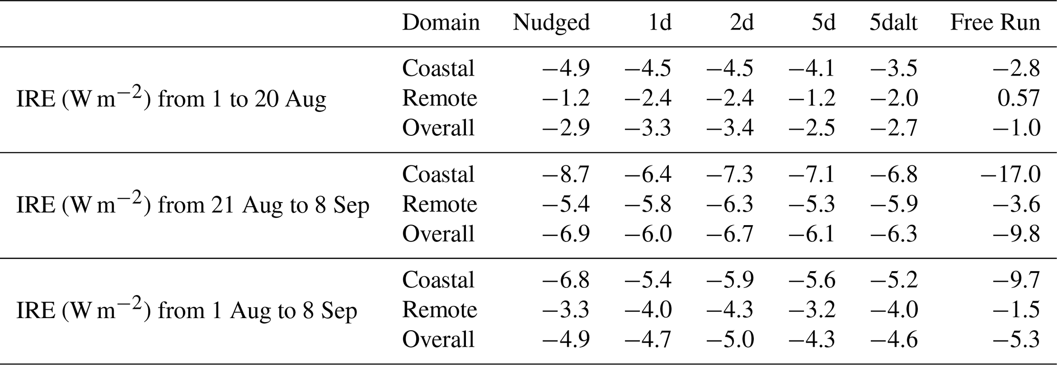
Our 2d IRE result of −5.9 W m⁻² over 1 August to 8 September 2017 is similar to that of Lu et al. (2018), who reported a −7.0 W m⁻² IRE cooling for the same overall domain from 1 August to 30 September 2014. Our Nudged IRE magnitudes are significantly stronger than those reported in Che et al. (2021) and Gordon et al. (2018). The difference is largely attributed to LWP, with LWP being represented more accurately with respect to observations in our UMv11.9 simulations relative to the UMv11.2 simulations of Che et al. (2021) and Gordon et al. (2018). Additionally, Che et al. (2021) and Gordon et al. (2018) assumed that background aerosol absorption is inconsequential in the calculation of REs, as discussed in Sect. 2.3. Here, we use an updated formulation that eliminates assumptions about background aerosol concentrations. We recalculated our results using the same assumptions as Gordon et al. (2018) and find that including background aerosol absorption introduced 1.2 W m⁻² of additional cooling into our Nudged IRE results. Since CRE remains unchanged between methods and SDRE is calculated as the difference between CRE and IRE, this update to background aerosol absorption has an equal and opposite impact on calculated SDRE results, introducing 1.2 W m⁻² of semi-direct warming.

Table 5 IRE (W m⁻²) averaged over each domain for 1–20 August, 21 August–8 September, and 1 August–8 September 2017.

4.5 Semi-direct radiative effects

Figures 16 and 17 show grid resolved SDRE calculated over ocean at TOA, according to Eq. (4), for each weather adjustment technique across the various domains and time spans. The full list of resulting magnitudes from all simulations, across every domain and time span, is shown in Table 6.

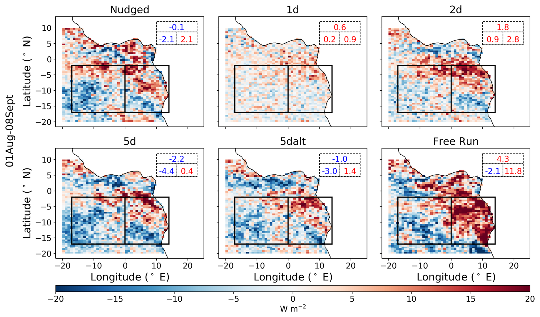
Figure 16 SDRE calculated according to Eq. (4) across all simulation sets and averaged over the SEA from 1 August to 8 September 2017. Values in the top right corner represent spatial averages of the overall (top), remote (left), and coastal (right) domains. Positive mean magnitudes are shown in red for warming, and negative mean magnitudes are shown in blue for cooling.

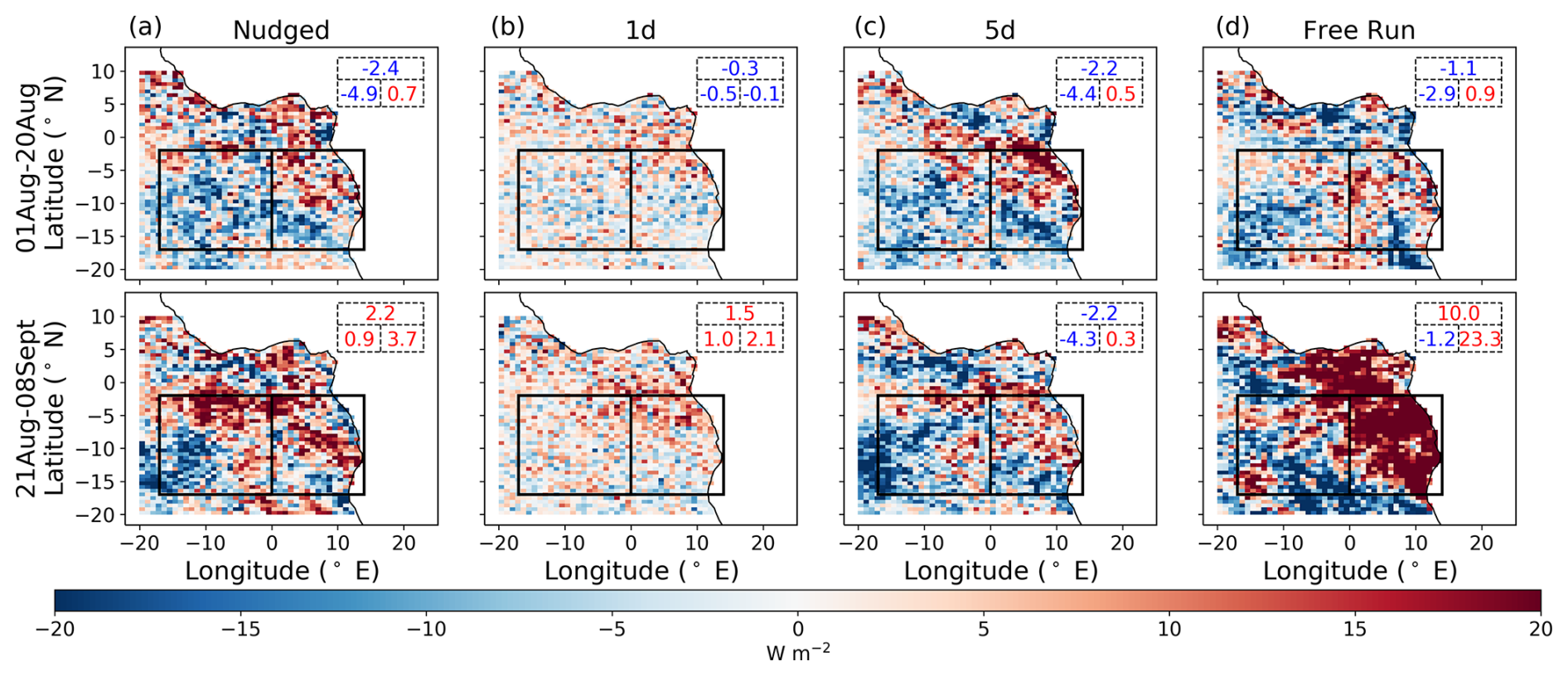
Figure 17 SDRE calculated according to Eq. (4) and averaged over the SEA for 1–20 August (top row) and 21 August–8 September (bottom row) for the Nudged (a), 1d (b), 5d (c), and Free Run (d) simulation sets. Values in the top right corner represent spatial averages of the overall (top), remote (left), and coastal (right) domains. Positive mean magnitudes are shown in red for warming, and negative mean magnitudes are shown in blue for cooling.

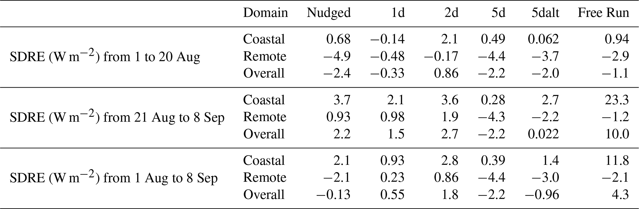
The overall SDRE varies substantially, both in magnitude and sign, between the simulation sets and over the spatial domain. The variation is especially pronounced in the remote domain from 21 August to 8 September. With nudged simulations, we calculate weaker semi-direct cooling than Che et al. (2021),and Gordon et al. (2018). The weaker cooling is likely mainly due to the different time period and spatial domain and to improved simulations of clouds. Compared to Che et al. (2021) and Gordon et al. (2018), the elimination of background aerosol assumptions also introduced an extra 1.2 W m⁻² of warming into our Nudged SDRE results, as discussed in Sect. 4.4.

Figures 16 and 17 also show the variability in SDRE between simulations is not from vastly different spatial distributions of SDRE between simulations but from differences in magnitudes. The SDRE is generally most positive in the north of the coastal box and most negative in the southwest of the remote box. The SDREs align well with the corresponding changes in LWP and CF in accordance with Eq. (4), as shown for Nudged in Fig. S17 of the Supplement. The changes in CF and LWP that contribute to the SDRE are locally substantially larger than those contributing to the IRE (up to around 15 % and 25 g m⁻² respectively) and are both significant and positive in the domain mean. These would therefore be expected to support a strong negative SDRE in the shortwave. Two key reasons why the SDRE is instead close to zero overall turn out to be the contribution from longwave radiation, discussed in Sect. 4.6, and the change in CDNC associated with absorption-induced changes in the altitude of the smoke plume, discussed in Sect. 4.7.

Our 2d results, which yield an overall positive SDRE, are opposite in sign to those of Lu et al. (2018), who observed a strongly cooling SDRE (over a different time period). It is possible that warming SDREs emerge in shorter forecasts than cooling SDREs: our 1d and 2d SDREs are warmings while 5d (and nudged) SDREs are coolings. However, the SDRE in the Free Run set is also positive and very large. We argue that the Free Run simulations are not sufficiently constrained to analysis, meaning that “butterfly effects” build up (Palmer, 2024), and the differences between simulations with and without smoke do not reflect the real SDRE. Conversely, SDRE in the 1d (Fig. 17) and 2d simulation sets (Table 6 or Fig. S18 of the Supplement) does not reach the same magnitudes as Nudged and 5d. This suggests that either the Nudged and 5d sets are insufficiently constrained to the analysis, leading to the same butterfly effects as in the Free Run, or the 1d and 2d simulations are too constrained, such that cloud and meteorological adjustments (for example, MBL height) to the smoke are not fully simulated. In Sect. 5, we argue that the latter explanation is more likely.

Table 6 SDRE (W m⁻²) averaged over each domain for 1–20 August, 21 August–8 September, and 1 August–8 September 2017.

4.6 Separating shortwave and longwave

Figure 18 shows the Nudged REs separated into shortwave and longwave components over the whole simulation from 1 August to 8 September. Shortwave (longwave) components are computed using only the shortwave (longwave) variables associated with Eqs. (1)–(4). The full effect is therefore the sum of the shortwave and longwave components. The results are qualitatively consistent across the simulation sets. The full list of component longwave magnitudes from all simulations across the full simulation time span from 1 August to 8 September is shown in Table S3 of the Supplement.

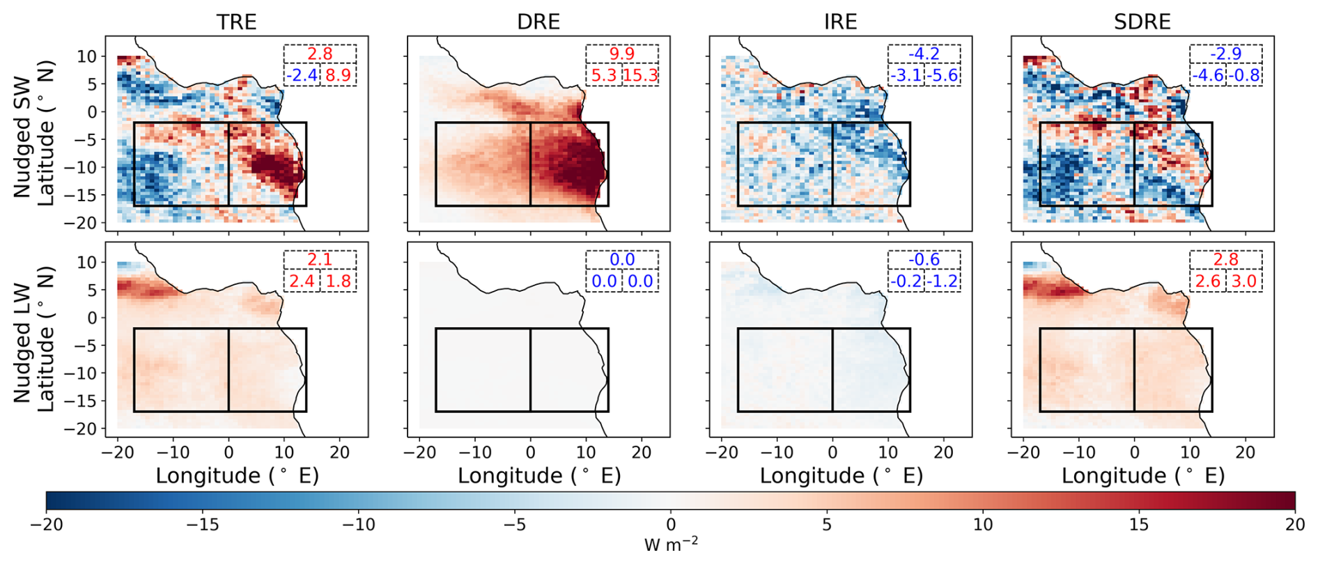
Figure 18 All nudged REs averaged over the SEA from 1 August to 8 September 2017, separated into shortwave (SW; top row) and longwave (LW; bottom row) components. Values in the top right corner represent spatial averages of the overall (top), remote (left), and coastal (right) domains. Positive mean magnitudes are shown in red for warming, and negative mean magnitudes are shown in blue for cooling.

Longwave REs are primarily influenced by the cloud fraction and the temperature at which clouds emit radiation, which is dictated by the height of the cloud layer. Our results are consistent in sign with those of Gordon et al. (2018), who found a LW IRE of −0.4 W m⁻² and LW SDRE of +2.3 W m⁻² when averaging across an area similar to our remote domain over five consecutively polluted days in August 2016. Our remote domain values are a LW IRE of −0.2 W m⁻² and a LW SDRE of +2.6 W m⁻², averaged over the whole simulation period. The relatively high LW RE suggests that smoke aerosols are influencing the height of the boundary layer and cloud tops. This height increase reduces the temperature of the cloud, lowering the amount of radiation they can emit to space and producing a positive LW RE. The increase in cloud top height is caused by BBA absorption and is visible in Fig. 19 below. The negative LW IRE may stem from increased radiative cooling due to the reduced cloud droplet size with the smoke present or from a change in cloud fraction; however, changes in cloud fraction (Fig. S15 of the Supplement) are very small. Since Eq. (3) uses two simulations without aerosol absorption, differences in cloud layer height between simulations are expected to be minimal.

4.7 Effect of aerosol absorption on cloud drop number concentration

Figure 19 shows a comparison of the vertical profiles of temperature, liquid water content, dry extinction, and in-cloud CDNC between Nudged_bb and Nudged_bbnoaa for the overall domain, averaged over 1 to 20 August and 21 August to 8 September. Our simulations show that the effect of aerosol absorption is to raise the altitude of the smoke layers, as observed by Johnson and Haywood (2023). The influence of radiative heating associated with absorption on the buoyancy of surrounding air masses is termed self-lofting (Radke et al., 1990). Self-lofting in our simulations leads to a substantial decrease in CDNC compared to simulations in which absorption is switched off. This decrease is comparable in magnitude to the change in CDNC associated with the IRE and is therefore large enough to have a significant radiative effect of its own.

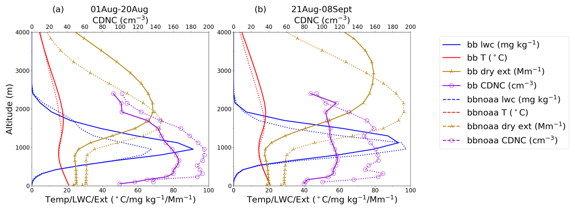
Figure 19 Mean vertical profiles of temperature (red), liquid water content (blue), dry extinction (gold), and in-cloud CDNC (purple) compared between Nudged_bb (solid) and Nudged_bbnoaa (dashed) in the overall domain. The comparison is separated into averages over two time spans: 1–20 August (a) and 21 August–8 September (b) 2017.

The impact of aerosol absorption on the smoke layer height can be identified by comparing dry extinction between simulations with and without aerosol absorption. Here, we see a 300–1000 m increase in the elevation of smoke with aerosol absorption. This is consistent with the findings of Johnson and Haywood (2023) who found that self-lofting elevates BBA from African fires by up to 1 km over the SEA. Self-lofting also has an impact on clouds, which can be identified by comparing liquid water content and CDNC in the MBL between simulations with and without aerosol absorption. The increase in liquid water with aerosol absorption highlights the mechanism of SDRE cooling, where aerosol absorption increases MBL stability and allows more moisture to accumulate within the MBL. CDNC at cloud top, however, decreases with aerosol absorption. The increased buoyancy caused by absorption elevates the smoke to heights further above the clouds. Smoke therefore mixes into the MBL less efficiently, and with less smoke mixing into clouds, there are not as many cloud droplets activated from BBA. Diamond et al. (2022) also compared simulations with and without absorption using WRF-CAM5 and found that the MBL contains less smoke when aerosol absorption is switched on, which is qualitatively consistent with our results.

Due to self-lofting, the change in CDNC caused by smoke is larger in the absence of absorption than in its presence. This finding has an implication for the formulas we used to disentangle BBA REs. With significantly larger CDNC in simulations without aerosol absorption, the IRE we calculate using Eq. (3), which uses simulations without aerosol absorption, is too negative; IRE cooling is overestimated. The SDRE computed using Eq. (4), which depends on the IRE magnitude calculated using Eq. (3) that overestimates IRE cooling, is therefore too positive; SDRE warming is overestimated. The overestimation applies to both the shortwave and longwave calculations. These findings highlight the difficulty of cleanly separating the IRE and SDRE using simulations without absorption. However, the more general cloud-mediated RE and the total RE remain unaffected by the use of simulations without aerosol absorption. Table 7 below shows cloud-mediated RE magnitudes from all simulations across every domain and time span. Cloud-mediated RE, calculated using Eq. (7), is likely to be more accurate than IRE using Eq. (3) (as seen in Table 5) and SDRE using Eq. (4) (as seen in Table 6).

The impact that aerosol absorption has on the height of the smoke plume also impacts our ability to cleanly separate the DRE into DRE_scattering and DRE_absorbing. However, since DRE is not very sensitive to CDNC, we do not expect the impact to be as strong. With more efficient mixing into the MBL without aerosol absorption, DRE_scattering, calculated by Eq. (5) using simulations without absorption, is likely underestimated as smoke is mixed into the MBL and subsequently lost more quickly than real absorbing smoke. Consequently, this would make DRE_absorbing, calculated by Eq. (6), likely an overestimation. The full DRE, however, remains unaffected, as Eq. (2) uses only simulations with aerosol absorption.

Table 7 CRE (W m⁻²) averaged over each domain for 1–20 August, 21 August–8 September, and 1 August–8 September 2017.

5 Conclusions

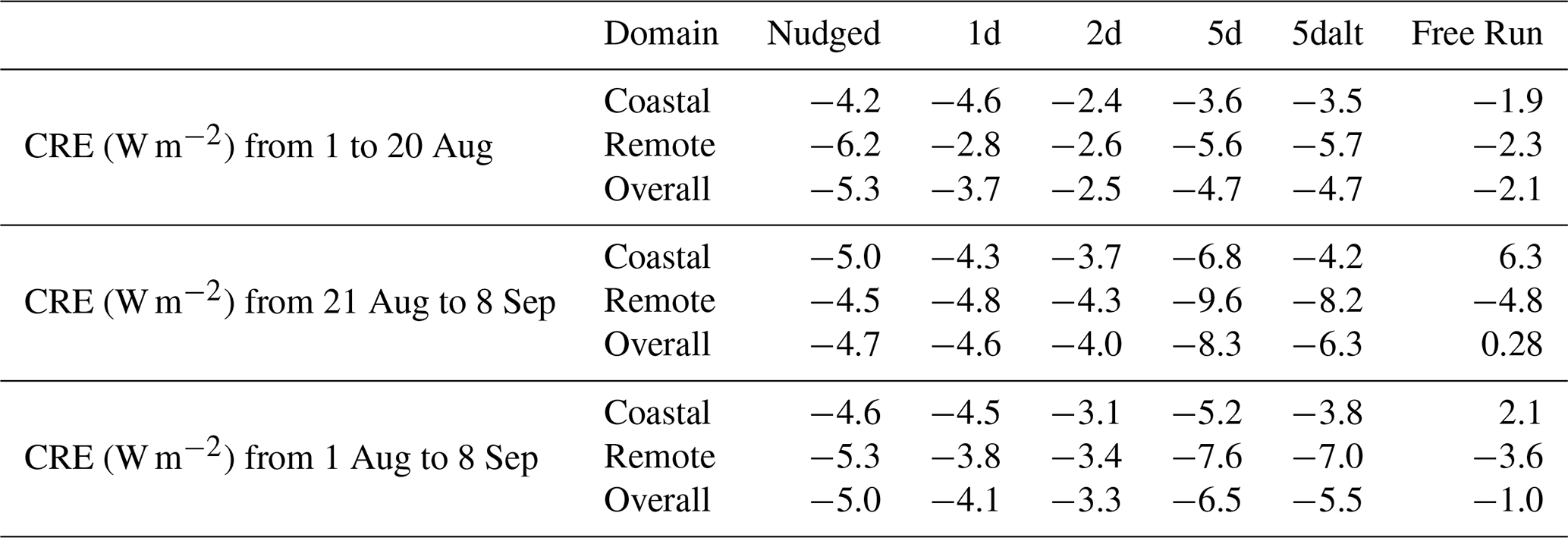
In this study, we quantified the total radiative effect (TRE) of smoke in the southeastern Atlantic Ocean (SEA) from 1 August to 8 September 2017 at TOA and its component direct radiative effect (DRE) and cloud-mediated radiative effect (CRE). We further disentangled these into component DRE warming, DRE cooling, the indirect radiative effect (IRE), and the semi-direct radiative effect (SDRE). Holding all else equal, we repeated our calculations using model setups that were used in recent studies to force meteorology to match observations. These setups include nudging horizontal winds above the boundary layer (Nudged), reinitializing at intervals of 1 d (1d), 2 d (2d), and 5 d (5d), another 5 d reinitialization starting on 3 August instead of 1 August (5dalt), and a control setup in which no forcing takes place after initialization on 1 August (Free Run). Calculations of TRE by Eq. (1) ranged from +3.0 to +7.9 W m⁻² depending on the forcing technique used, displaying a net warming over the SEA overall. The variability between simulation sets is dominated by the SDRE. The variation in our results suggests that the method used to force meteorological agreement with observations may contribute substantially to the variation in the results of previous studies quantifying BBA RE magnitudes in the SEA.

Since REs are sensitive to both aerosol and cloud properties, it is critical that simulations are in reasonably close agreement with observations. We evaluated our model setup using the CLARIFY and ORACLES aircraft measurements, LASIC measurements, and the MODIS and CERES satellite measurements. Of variables likely to impact smoke REs, the model simulates meteorology (boundary layer height, temperature, and relative humidity), clouds, and aerosol absorption relatively well compared to the state of the art documented in model intercomparisons. However, biases in aerosol extinction are substantial, and biases in any of these variables may impact aerosol REs to some extent.

Differences in radiative effects between simulations with different meteorological forcing methods reflect differences in the characteristic timescales for the three radiative effects. The DRE is instantaneous, and the Twomey effect is nearly instantaneous. Adjustments to cloud fraction and liquid water path by changes in droplet sedimentation and precipitation rates are also relatively fast compared to semi-direct cooling. Recent research suggests that adjustment-driven IREs in real stratocumulus clouds equilibrate to aerosol changes with a characteristic timescale of around 20 h (Glassmeier et al., 2021). For the SDRE, there are two cloud alteration mechanisms: the cloud thickening mechanisms of SDRE cooling and the cloud thinning mechanism of SDRE warming. A popular explanation for the change in cloud optical thickness due to the SDRE suggests that as carbonaceous aerosols absorb radiation above clouds, they suppress entrainment between the free troposphere and the low-level marine clouds within the boundary layer. The result is an accumulation of moisture in the MBL and a thickening of the cloud. Conversely, warming SDREs result from heating in the boundary layer, directly evaporating clouds. Our simulations indicate that, unsurprisingly, the adjustment of the average moisture level in the boundary layer takes longer than Twomey-dominated indirect effects, as IREs agree between simulation sets but SDREs do not.

Any study seeking to quantify short-term radiative effects of absorbing aerosols must compromise between the need to avoid artifacts of chaotic model internal variability and the need to allow differences between simulations to emerge. In the SEA, air masses carrying smoke usually take approximately six days to reach Ascension Island (Fig. 1) from the African coast (Dobracki et al., 2025), though occasionally as few as four days (Zuidema et al., 2018; Gordon et al., 2018). We therefore expect perturbations to the marine boundary layer (for example, to its height or inversion strength) due to smoke to build up over up to six days. However, smoke far above the boundary layer has little effect on clouds (Herbert et al., 2020), so we expect six days to be an upper limit on these perturbations to the boundary layer. In our 1d simulations, we allowed no spin-up; in 2d, there is one day, and in 5d, there are two days. In the 2d simulation, air arriving at Ascension Island has had between one and three days to evolve and modify the boundary layer according to whether or not it contains smoke. We might therefore expect realistic SDREs in the coastal domain, which takes around one day to traverse from the African coast but not in the remote box. In the 1d simulation, there are between zero and one day for the meteorology to be influenced by smoke or the lack of smoke, so we would not expect realistic SDREs anywhere. In the 5d simulation, there is between two and seven days for smoke or lack of smoke to influence the boundary layer, and we conclude that the SDREs should be realistic most of the time (though potentially still interrupted by reinitialization). However, better simulation setups may still exist. For example, a simulation reinitialized every two days and run for seven days (allowing five days of spin-up) would allow a more consistently long time period (between five and seven days) for smoke to influence meteorology. However, this setup would be more computationally expensive, and similarities in results between 5d and 5dalt suggest that internal variability is not yet a major problem in the 5d setup.

The Free Run simulation can be thought of as both a control for our experiment and a reinitialized simulation where the forecast length matches the whole simulation time period. The results highlight both the importance of using weather adjustment techniques on shorter simulation time spans and the pitfalls of selecting too long an interval between reinitialized forecasts. A model evaluation of the Free Run simulation can be found in Figs. S2–S14 of the Supplement. In summary, the Free Run biases are in the same direction but substantially more exaggerated in magnitude than those of Nudged_bb and 5d_bb. Comparing 1 to 20 August and 21 August to 8 September, the IRE and SDRE magnitudes in the Free Run are 1 order of magnitude larger in the latter time period relative to the former and far larger in this latter time period than those in our other simulations. This result strongly suggests that simulated meteorology in the smoke and no-smoke simulations diverged throughout the simulation. This divergence is likely due to “butterfly effects” or chaotic internal variability and would exist between any pair of simulations with a small difference between them that influences their integration of the Navier–Stokes equations (Palmer, 2024; Lorenz, 1969). We cannot be sure that such effects are not negligible in our other simulations, but we can get an indication of their likely size by examining differences across an initial-condition ensemble. Two members in such an ensemble are 5d and 5dalt. Using only two members is too small a sample to be statistically robust, but their results still suggest that the 5d setup may be a reasonable choice.

In Sect. 4.7, we found BBA self-lofting, in which BBA absorption increases the buoyancy of the surrounding air masses and leads to less smoke mixing into the clouds, thereby reducing cloud droplet number concentration and making the clouds less bright. The use of simulations without aerosol absorption to disentangle the CRE into the IRE and SDRE therefore introduces a bias in our IRE and SDRE results, because BBA absorption has an impact on both the IRE (by changing CDNC) and the SDRE. The bias presents itself in our results as an overestimation of IRE cooling and an overestimation of SDRE warming. Although this bias is present in our IRE and SDRE, the CRE and TRE remain unaffected and still vary between meteorological forcing methods. We therefore expect that our conclusions regarding the characteristic timescales of radiative effects are still applicable.

We conclude from our study that (a) running reinitialized forecasting simulations that are too short (with three-day-long forecasts or less) biases the total simulated smoke radiative effect (TRE) by influencing the SDRE and (b) smoke aerosol absorption influences simulated CDNC by changing the height of smoke plumes, biasing IREs that are calculated with absorption switched off. While our investigation is not exhaustive, nudging horizontal winds above the BL or running seven-day-long forecasts with a two-day spin-up appear to be the most robust techniques for quantifying RE magnitudes over shorter time periods in the SEA, on the order of weeks to months. We recommend these techniques for future similar research, as the appropriate choice for forecasting and spin-up length may depend on wind strength. Our results are pertinent to quantifying BBA REs in the SEA, but we also expect the same logic to be relevant to understanding the short-term radiative effects of absorbing aerosols elsewhere.