Thermospheric nitric oxide is modulated by the ratio of atomic to molecular oxygen and thermospheric dynamics during solar minimum

The formation of nitric oxide (NO) by geomagnetic activity and EUV photoionization in the upper mesosphere and lower thermosphere, and its subsequent impact on ozone, contributes to the natural forcing of the climate system, and has been recommended to be included in chemistry-climate model experiments since CMIP6. We compare NO concentrations in the mesosphere and thermosphere simulated by five high-top chemistry-climate models – WACCM-X, EMAC, HAMMONIA, WACCM-D and KASIMA – with satellite observations during a period of low geomagnetic and solar forcing in January 2010. We find disagreements ranging from several orders of magnitude in the high-latitude winter lower thermosphere to about one order of magnitude in the low-latitude thermosphere. Possible reasons for this are explored by analyzing formation and loss reactions of NO at 12:00 UT on 9 January 2010. Two processes that interact with each other are identified as likely sources of these discrepancies, quenching of N(²D) by atomic oxygen in the mid-thermosphere, and meridional transport and mixing from the mid-thermosphere to the lower thermosphere. In the mid-thermosphere, the amount of atomic oxygen available from dissociation of molecular oxygen balances N(⁴S) and N(²D) via quenching of N(²D). N(⁴S) can then be transported or mixed into the lower thermosphere, where it efficiently destroys NO, leading to lower values of NO there. In winter, downward and poleward transport of N(⁴S) from the low and mid-latitude middle thermosphere into the high-latitude lower thermosphere modulates the NO lifetime. This transport is affected by gravity waves, and therefore depends on each models' gravity wave drag scheme and their resolved gravity wave spectra.

1 Introduction

Precipitating energetic particles have been recognized as a source of NO in the high-latitude upper stratosphere, mesosphere and lower thermosphere since the 1960s (e.g., Nicolet, 1965; Crutzen, 1975), recent reviews can be found in Sinnhuber et al. (2012), Mironova et al. (2015), and Baker et al. (2018). Similar processes also lead to the formation of NO in the low and mid-latitude uppermost mesosphere and lower thermosphere related to the absorption of solar electromagnetic radiation in the EUV and X-ray range (e.g., Watanabe et al., 1953; Barth, 1992; Marsh et al., 2004; Pettit et al., 2019). During polar winter, NO is long-lived and can be transported down from its source regions in the mesosphere and lower thermosphere into the upper stratosphere, contributing to ozone loss there (Funke et al., 2014; Randall et al., 2007; Sinnhuber et al., 2018). As ozone dominates radiative heating in the illuminated upper stratosphere and lower mesosphere and also contributes to radiative cooling, these changes in ozone initiate a chemical-radiative-dynamical coupling which even appears to affect large tropospheric weather systems in high-latitude winter (Seppälä et al., 2009; Rozanov et al., 2012; Maliniemi et al., 2014, 2019). This so-called indirect effect of energetic particle precipitation (EPP) therefore contributes to the natural variability of the climate system, and consequently has been recommended to be included in climate model reconstructions and projections since CMIP6 (Matthes et al., 2017; Funke et al., 2024).

The starting point of the EPP indirect effect is the formation of NO mainly in the upper mesosphere and lower thermosphere by auroral and magnetospheric electron precipitation at high latitudes, as well as by absorption of EUV and X-ray radiation. Dissociation and dissociative ionization of N₂ by collisions with energetic particles or absorption of EUV/X-ray radiation form atomic nitrogen in the ground (N⁴S) or first excited (N²D) state (see, e.g., Sinnhuber et al. (2012) and references therein¹):

$$\begin{array}{}\text{(R1)}& {\displaystyle }{\mathrm{N}}_{\mathrm{2}}+hv,e^{*}⟶\mathrm{2}\mathrm{N}{(}^{\mathrm{2}}\mathrm{D}),\mathrm{N}{(}^{\mathrm{4}}\mathrm{S})\text{(R2)}& {\displaystyle }{\mathrm{N}}_{\mathrm{2}}+hv,e^{*}⟶{\mathrm{N}}^{+}+\mathrm{N}{(}^{\mathrm{2}}\mathrm{D}),\mathrm{N}{(}^{\mathrm{4}}\mathrm{S}).\end{array}$$

Both the ground state N(⁴S) and the first excited state N(²D) of atomic nitrogen can react with molecular oxygen to form NO (Barth, 1992):

$$\begin{array}{}\text{(R3)}& {\displaystyle }\mathrm{N}{(}^{\mathrm{4}}\mathrm{S})+{\mathrm{O}}_{\mathrm{2}}⟶\mathrm{NO}+\mathrm{O}\text{(R4)}& {\displaystyle }\mathrm{N}{(}^{\mathrm{2}}\mathrm{D})+{\mathrm{O}}_{\mathrm{2}}⟶\mathrm{NO}+\mathrm{O}\end{array}$$

At temperatures below 400 K, Reaction (R4) is much faster than Reaction (R3), and NO is mainly formed via Reaction (R4). However, the rate constant of Reaction (R3) is strongly temperature dependent, and this reaction becomes a significant source of NO at temperatures above ≈400 K (see also discussion in Sinnhuber and Funke, 2019). Quenching of N(²D) by atomic oxygen or electrons has also been discussed:

$$\begin{array}{}\text{(R5)}& {\displaystyle }\mathrm{N}{(}^{\mathrm{2}}\mathrm{D})+\mathrm{O}⟶\mathrm{N}{(}^{\mathrm{4}}\mathrm{S})+\mathrm{O},\text{(R6)}& {\displaystyle }\mathrm{N}{(}^{\mathrm{2}}\mathrm{D})+e^{-}⟶\mathrm{N}{(}^{\mathrm{4}}\mathrm{S})+e^{-}.\end{array}$$

N(²D) also relaxes to N(⁴S) by fluorescence:

$$\begin{array}{}\text{(R7)}& \mathrm{N}{(}^{\mathrm{2}}\mathrm{D})⟶\mathrm{N}{(}^{\mathrm{4}}\mathrm{S})+hv\end{array}$$

(see summaries and references in Barth, 1992; Sinnhuber et al., 2012; Verronen et al., 2016).

Another source of NO is the formation of NO⁺ by ion chemistry reactions summarized, e.g., in Barth (1992), Sinnhuber et al. (2012), and Sinnhuber and Funke (2019):

$$\begin{array}{}\text{(R8)}& {\displaystyle }{\mathrm{N}}_{\mathrm{2}}^{+}+\mathrm{O}⟶{\mathrm{NO}}^{+}+\mathrm{N}{(}^{\mathrm{2}}\mathrm{D}),\mathrm{N}{(}^{\mathrm{4}}\mathrm{S}),\text{(R9)}& {\displaystyle }{\mathrm{N}}^{+}+{\mathrm{O}}_{\mathrm{2}}⟶{\mathrm{NO}}^{+}+\mathrm{O},\text{(R10)}& {\displaystyle }{\mathrm{O}}_{\mathrm{2}}^{+}+{\mathrm{N}}_{\mathrm{2}}⟶{\mathrm{NO}}^{+}+\mathrm{NO},\text{(R11)}& {\displaystyle }{\mathrm{O}}^{+}+{\mathrm{N}}_{\mathrm{2}}⟶{\mathrm{NO}}^{+}+\mathrm{N}{(}^{\mathrm{2}}\mathrm{D}),\mathrm{N}{(}^{\mathrm{4}}\mathrm{S}),\end{array}$$

followed by recombination again forming either N(²D) or N(⁴S),

$$\begin{array}{}\text{(R12)}& {\mathrm{NO}}^{+}+e^{-}⟶\mathrm{N}{(}^{\mathrm{2}}\mathrm{D}),\mathrm{N}{(}^{\mathrm{4}}\mathrm{S})+\mathrm{O}.\end{array}$$

NO⁺ can also be formed by photoionization of NO (Barth, 1992):

$$\begin{array}{}\text{(R13)}& \mathrm{NO}+hv⟶{\mathrm{NO}}^{+}+e^{-}.\end{array}$$

The main loss reactions for NO are the photolysis reaction,

$$\begin{array}{}\text{(R14)}& \mathrm{NO}+hv⟶\mathrm{N}{(}^{\mathrm{4}}\mathrm{S})+\mathrm{O},\end{array}$$

and the scavenging reaction with N(⁴S),

$$\begin{array}{}\text{(R15)}& \mathrm{NO}+\mathrm{N}{(}^{\mathrm{4}}\mathrm{S})⟶{\mathrm{N}}_{\mathrm{2}}+\mathrm{O},\end{array}$$

(see, e.g., Barth, 1992; Marsh et al., 2004; Sinnhuber et al., 2012; Sinnhuber and Funke, 2019). The amount of NO formed due to particle or photo-ionization thus depends on the rate of ionization (Reactions R1, R2). It also depends on temperature (Reaction R3) and the partitioning between N(²D) and N(⁴S) formed (Reactions R3, R4). If the partitioning is in favour of N(²D), net NO formation is high, but if it is in favour of N(⁴S), enhanced loss due to Reaction (R15) could lead to a saturation effect with little net NO formation (Sinnhuber et al., 2012). Reactions (R8) and (R12) are expected to preferentially or solely produce N(²D), while Reaction (R11) produces mainly N(⁴S), and Reactions (R1) and (R2) produce comparable amounts of N(²D) and N(⁴S) with partitionings between 0.4 and 0.6 (see, e.g., summaries and references in Barth, 1992; Sinnhuber et al., 2012; Verronen et al., 2016).

For chemistry-climate models with the top in the upper mesosphere, the EPP indirect effect is well described by an upper boundary condition prescribing either the flux of NO through the model top or the NO density at the model top, developed by Funke et al. (2016) based on ten years of MIPAS observations as recommended for the Coupled Model Intercomparison Project phases 6 and 7, CMIP6 and CMIP7 (Matthes et al., 2017; Funke et al., 2024). Models using an NO upper boundary condition based on observations have been shown to reproduce NO_y² due to the EPP indirect effect very well (Sinnhuber et al., 2018; Arsenovic et al., 2019). High-top models with their top in the source region of auroral and EUV ionization, which self-consistently consider NO formation by atmospheric ionization, agree morphologically well, but mostly fail to reproduce the observed amount of NOy transported into the stratosphere (Smith-Johnsen et al., 2017; Funke et al., 2017; Sinnhuber et al., 2018; Pettit et al., 2019). Recently, a model-measurement intercomparison was carried out for a geomagnetic storm in April 2010 incorporating four high-top models extending into the lower thermosphere. This intercomparison has shown variations of up to one order of magnitude from model to model in the lower thermosphere even when using the same EUV and particle forcing (Sinnhuber et al., 2022). The overestimation of NO in the tropical lower thermosphere by three out of the four models compared to observations was tentatively interpreted as an overestimation of the rate of EUV photoionization provided by the parameterization of Solomon and Qian (2005) used in those models. A similar overestimation of low-latitude lower thermospheric NO was shown in a comparison of results of one model with observations of NO (Siskind et al., 2019). That study concluded that the overestimation was an indication of problems with the photochemistry since electron densities – another indicator of atmospheric ionization – were underestimated by the model at the same time. The large spread between models in Sinnhuber et al. (2022) was tentatively interpreted as being due to differences in thermospheric temperature affecting the rate of formation of NO via Reaction (R3). However, as the main focus of the Sinnhuber et al. (2022) intercomparison was on the impact of medium-energy electron precipitation on mesospheric composition during a geomagnetic storm, thermospheric temperature effects were not investigated further there.

Here, we follow up on the results of Sinnhuber et al. (2022) by investigating in detail the roles of different reaction pathways forming and destroying NO using a snapshot of model results at one timestep. In Sect. 2, models, model experiments, and satellite data used in the study are described. Results are presented in Sect. 3, and implications are discussed in Sect. 4.

2 Models, model experiments, and satellite observations

2.1 Chemistry-climate Models

The same models participated in this follow-up experiment as in the Heppa III intercomparison discussed in Sinnhuber et al. (2022): WACCM-D, EMAC, HAMMONIA, and KASIMA. Additionally, results of WACCM-X are used. WACCM-X shares the same chemistry code and derivation of ionization rates as WACCM-D, but has an extended model top and no detailed D-region ion chemistry. All participating models are high-top models with the model top well above the mesopause. All models use the same parameterization of EUV photoionization based on Solomon and Qian (2005) and most use particle impact ionization rates from the AISstorm model (see Sect. 2.2). Model tops vary from 115 km (KASIMA) to 500 km (WACCM-X) and the derivation of auroral ionization rates and implementation of ion chemistry differ as well (see summary in Table 1 and detailed descriptions of all models below).

Table 1 Participating models.

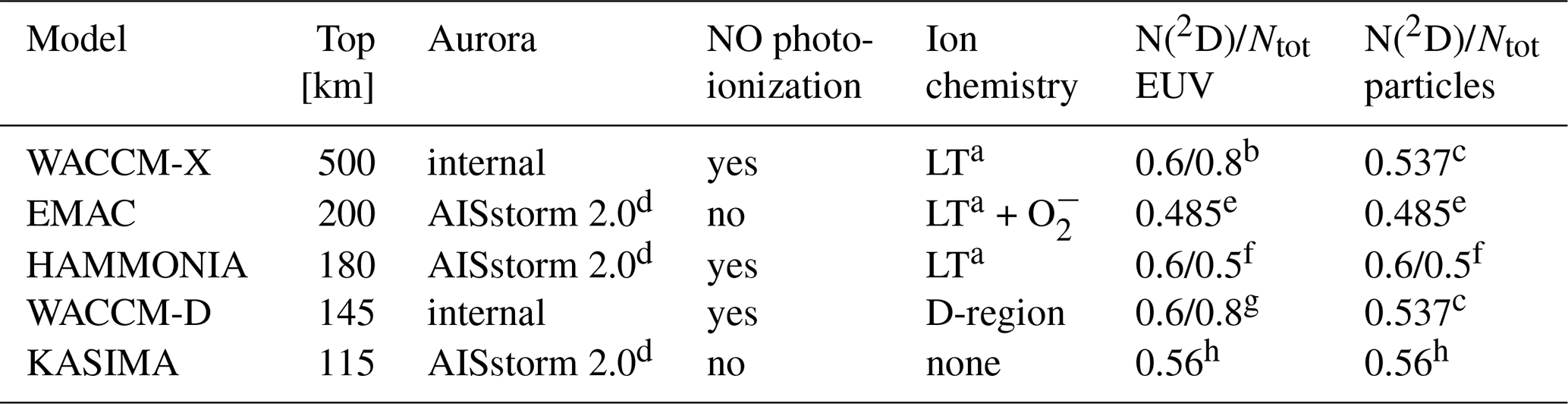
^a Lower thermosphere ion chemistry with five positive ions and electrons. ^b Depending on wavelength. ^c Verronen et al. (2016). ^d AISstorm 2.0: see Sect. 2.2. ^e Assuming the partitioning of Porter et al. (1976) for photoionization and particles. ^f Dissociation and dissociative ionization as described in Kieser (2011). ^g Dissociation and dissociative ionization. ^h Assuming the partitioning of Jackman et al. (2005) for photoionization and particles, and assuming that the formation of NO equals the formation of N(²D).

WACCM-D: The Whole Atmosphere Community Climate Model Version 6 (WACCM6) is a chemistry-climate general circulation model that extends from the surface to about 6 × 10⁻⁶ hPa (∼ 140 km). The model horizontal resolution is 0.9° latitude by 1.25° longitude. A detailed description of the model physics in the MLT (mesosphere–lower thermosphere) region is provided by Marsh et al. (2007). WACCM6 incorporates both the orographic and nonorographic (convective and frontal) gravity wave drag parametrisation (Richter et al., 2010). Here, we use WACCM6 in the specified dynamics configuration named “FWmadSD” which is forced with meteorological fields (temperature and winds) from Modern-Era Retrospective analysis for Research and Applications (MERRA2, Molod et al., 2015). Middle atmosphere D-region chemistry mechanism (MAD) is based on the Model for Ozone and Related Chemical Tracers, Version 3 (Kinnison et al., 2007). It represents chemical and physical processes in the troposphere through to the lower thermosphere. In addition to a six constituent ion chemistry model (O⁺, O${}_{\mathrm{2}}^{+}$, N⁺, N${}_{\mathrm{2}}^{+}$, NO⁺, and electrons) that represents the E-region ionosphere, the MAD mechanism adds 15 positive and 21 negative ions with the aim to better reproduce the observed effects of energetic particle precipitation in the mesosphere and stratosphere (Verronen et al., 2016). For the solar spectral irradiance, geomagnetic indices, ion-pair production rates by galactic cosmic rays, solar protons, and medium-energy electrons, WACCM6 uses the CMIP6 solar and geomagnetic forcing as described in Matthes et al. (2017). For lower-energy electrons in the auroral regions, the model utilizes the auroral oval model by Roble and Ridley (1987). Photoionization and heating rates at wavelengths shorter than Lyman-α are based on the parameterization of Solomon and Qian (2005). Upper boundary conditions for temperature, H, O, O₂, N(⁴S) and N₂ are specified from the MSIS empirical model (Picone et al., 2002). NO at the upper boundary is specified from the Nitric Oxide Empirical Model NOEM (Marsh et al., 2004, 2007).

WACCM-X is a superset of WACCM6 with its top boundary in the upper thermosphere (4.5 × 10⁻¹⁰ hPa, or ∼ 500 km). It shares the same dynamics, physics and chemistry with WACCM6 up to the lower thermosphere, though the version of WACCM-X used in this study does not include D-region chemistry. At higher altitudes, the species-dependent dynamics, thermospheric and ionospheric energetics, ionospheric electrodynamics and transport are included in WACCM-X (Liu et al., 2010, 2018, 2024b).

For the simulation used here, the high latitude electric potential and ion convection patterns are specified according to Heelis et al. (1982) driven by 3-hourly Kp input. No gravity wave parameterization is applied above ∼ 120 km, because its formulation is based on linear saturation theory, which is no longer valid there. Forcing data are applied in the same way as in WACCM-D with the exception of medium-energy electron ionization, which is included in the Snapshot model experiment, but not in the Long model experiment (see Sect. 2.3).

EMAC: The ECHAM/MESSy Atmospheric Chemistry model EMAC is an atmospheric composition-climate model which includes sub-models describing a wide range of atmospheric processes (Jöckel et al., 2010). EMAC uses the second version of the Modular Earth Submodel System (MESSy2) to link multi-institutional computer codes. The core atmospheric model is ECHAM5 (Roeckner et al., 2006). For the present study we used ECHAM5 version 5.3.02 and MESSy version 2.55.0 in upper atmosphere mode, with 74 vertical layers and a model top height of ≈ 220 km ($\mathrm{3}\times {\mathrm{10}}^{-\mathrm{7}}$ hPa, EMAC submodule EDITH). The horizontal resolution is T42, corresponding to a resolution of about 2.8° × 2.8° in latitude and longitude. The model is nudged to the ECMWF ERA interim reanalysis data from the surface up to 1 hPa with decreasing nudging strength in a transition region in the six levels above. For orographic gravity waves, the parameterization of Lott and Miller (1997) is used. For non-orographic gravity waves, the Hines parameterization is used (Hines, 1997) in a set-up which allows propagation of gravity waves with ≈ 126 km horizontal wavelength and less than 12 km vertical wavelength into the lower thermosphere. Submodules RAD and RAD-FUBRAD are used for radiative heating and cooling rates (Roeckner et al., 2003; Dietmüller et al., 2016), using the wavelength grid provided by FUBRAD for UV radiative heating in the upper mesosphere and thermosphere (Nissen et al., 2007; Kunze et al., 2014). For gas-phase reactions the submodule MECCA is used (Sander et al., 2011a, b), and photolysis rates are calculated with the JVAL submodule (Sander et al., 2014) which includes a parameterization for O₂ photodissociation in the Lyman-α range, but not in the Schumann-Runge bands and continuum. For NO photolysis, the parameterization from Allen and Frederick (1982) is used without correction for self-absorption. For sensitivity studies, the O₂ photodissociation in the Schumann-Runge bands was implemented following Minschwaner et al. (1993), the O₂ photodissociation in the Schumann-Runge continuum was implemented with the same parameterization as used in KASIMA, but without consideration of the temperature dependence (sensitivity experiments SRBC, see Sects. 2.3 and 3.2). Particle impact ionization rates for auroral electrons, auroral and solar protons and heavier ions are provided by 2-hourly results from the AISstorm 2.0 ionization model on the EMAC latitude/longitude and pressure grid. EUV and X-ray photoionization rates are calculated based on the parameterization of Solomon and Qian (2005). A simple ion chemistry scheme is used to calculate the impact of particle impact and photoionization on the neutral composition and consider O${}_{\mathrm{2}}^{+}$, N${}_{\mathrm{2}}^{+}$, O⁺, N⁺, NO⁺, electrons and O${}_{\mathrm{2}}^{-}$. The latter is used as a proxy for negative charge in the stratosphere and mesosphere.

HAMMONIA: the Hamburg Model of the Neutral and Ionized Atmosphere (HAMMONIA) is a chemistry-climate model that calculates interactions of atmospheric chemistry, radiation and dynamics from the surface to $\mathrm{3.4}\times {\mathrm{10}}^{-\mathrm{7}}$ hPa (∼ 200–250 km). It consists of the ECHAM5 general circulation model (Roeckner et al., 2006) coupled to the MOZART3 chemistry module (Kinnison et al., 2007) and extended to the thermosphere (Schmidt et al., 2006; Meraner et al., 2016). HAMMONIA has 118 vertical levels and a T63 horizontal resolution, corresponding to about 1.9° × 1.9° in latitude and longitude. For nudging, the model uses ECMWF ERA interim reanalysis data from 850 up to 1 hPa with an upper and lower transition zones. As in EMAC, for the orographic and and non-orographic gravity waves the model uses parameterizations of Lott and Miller (1997) and Hines (1997), respectively. Solar radiation is treated by a 6-band parameterization below 30 hPa (Cagnazzo et al., 2007) and by a 200–800 nm TUV parameterization (Madronich and Flocke, 1999) above, which is also used for photolysis calculations. In a 120–200 nm spectral region, the model uses various parameterizations for the O₂ photolysis including Schumann-Runge bands and continuum (for details, see Schmidt et al., 2006) and Minschwaner and Siskind (1993) for the NO photolysis. The ion chemistry consists of 13 ion-neutral reactions and 5 ion-electron recombinations involving O${}_{\mathrm{2}}^{+}$, N${}_{\mathrm{2}}^{+}$, O⁺, N⁺, NO⁺, and electrons. This scheme is driven by the particle-induced ionization rates provided by the ionization model AISstorm 2.0 and by solar EUV and X-rays, following Solomon and Qian (2005). Joule heating and ion drag contribution to thermospheric temperature and wind tendencies are parameterized based on Zhu et al. (2005).

KASIMA: In this study we use the KArlsruhe SImulation Model of the middle Atmopshere (Kouker et al., 1999) in the version described in Sinnhuber et al. (2022). The model solves the meteorological basic equations in spectral form in the altitude range between 300 hPa and $\mathrm{3.6}\times {\mathrm{10}}^{-\mathrm{5}}$ hPa with the pressure height $z=H\log (p/p_{\mathrm{0}})$ (H=7 km and p₀=1013.25 hPa) as a vertical coordinate. It uses radiative forcing terms for UV-Vis and IR, and a gravity wave drag scheme. The model is relaxed (nudged) to ERA-Interim meteorological analyses (Dee et al., 2011) between the lower boundary of the model and 1 hPa. A full stratospheric chemistry package that includes heterogeneous processes is adapted to include source terms related to particle and photon ionization. The ionization rates are taken from the AISstorm ionization model for the particle contribution, plus the photoionization based on the parameterization of Solomon and Qian (2005), which has been included in the model for this study. For the production of HO_x per ion pair the parameterization of Solomon et al. (1981) is used. For the production of NO_x, 0.7 NO molecules and 0.55 N atoms in ground state are produced per ion pair.

2.2 Ionization model AISstorm 2.0

The Atmospheric Ionization during Substorms model AISstorm is a numerical model designed to calculate atmospheric ionization rates due to precipitating particles with high spatial resolution, improving upon its predecessor AIMOS (Wissing and Kallenrode, 2009) by specifically addressing substorm periods. AISstorm computes 3D ionization rates for precipitating protons, electrons, and alpha particles at a temporal resolution of 30 min. The model employs a sorting algorithm to allocate observations from polar-orbiting POES and Metop satellites into horizontal precipitation cells. To achieve this, AISstorm utilizes data from the TED and MEPED detectors and incorporates high-energy proton and alpha particle data from the SEM detectors on GOES satellites for the polar cap.

The energy range covered includes 154 eV to 500 MeV for protons, 154 eV to 300 keV for electrons, and 4 to 500 MeV for alpha particles. Mean flux maps were generated from 18 years of satellite data (2001–2018), categorized by Kp level, geomagnetic APEX (Richmond, 1995), magnetic local time (MLT) location with up to 1° latitude by 3.75° longitude resolution, and substorm activity. Each flux map illustrates a typical spatial pattern of particle precipitation for a single particle channel on a global scale. Typical average flow maps are presented in Yakovchuk and Wissing (2019). The effective flow for a 30 min interval is determined by scaling precipitation maps with direct measurements at that time, focusing on areas with high flux values (e.g., auroral oval) to minimize the impact of noise in real-time data.

For each interval, the ionization profile is calculated using the Monte Carlo method (Agostinelli et al., 2003; Schröter et al., 2006), with atmospheric parameters derived from the HAMMONIA (Schmidt et al., 2006) and NRLMSISE-00 (Picone et al., 2002) models.

2.3 Model experiments

Two main model experiments were set up and carried out by all models:

• For the Long experiment, model runs were carried out from 1 January to 31 December 2010, with at least one year of spinup-time before January 2010. Model output was daily mean, zonal mean values of NO on the model pressure and latitude grids from 1 January to 31 December 2010, providing one year of data. with a one-year spinup. The aim of this model experiment was to provide a spinup for the Snapshot experiment as well as a statistically more robust evaluation of the models performance in reproducing lower thermosphere NO compared to observations. A comparison of the full year 2010 compared to satellite observations is provided in the Sect. S2.1 and Fig. S1 of the Supplement.

• The Snapshot model experiment branches off from the Long experiment, with output at 12:00 UT on 9 January 2010 on the models latitude, longitude and pressure grid. This allows a detailed analysis of the photochemical processes related to atmospheric ionization, in particular NO, N(⁴S), and electron density. 9 January 2010 was chosen as representing Northern hemisphere mid-winter covered by MIPAS UA observations. For EMAC, two model experiments were carried out as a test of sensitivity, with (SRBC) and without (Snapshot) O₂ photodissociation in the Schumann-Runge bands and continuum as described in Sect. 2.1.

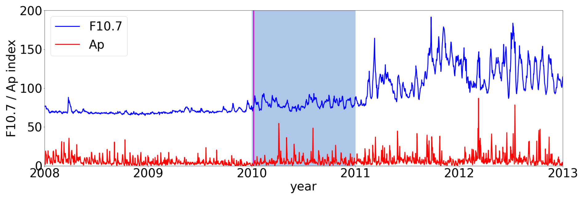
Figure 1 Daily F10.7 and Ap index for the period 2008–2013 from the CMIP6 forcing data-set. The blue box marks the period of the Long model run, the magenta line marks 9 January 2010, the date of the Snapshot model experiment.

The year 2010 was chosen as an extension of the Heppa III period in April 2010 (Nesse et al., 2022; Sinnhuber et al., 2022). It is at the end of an extended solar minimum with very low solar and geomagnetic activity, see Fig. 1. Moderate geomagnetic activity starts again in the second quarter of 2010 with auroral substorms and a moderate geomagnetic storm in April 2010, but EUV and X-ray fluxes remain low throughout the whole year. On the day of the Snapshot model run, EUV and auroral forcing are both relatively low.

2.4 NO observations

To evaluate the models' performance in the lower thermosphere, model results are compared against satellite observations of NO.

MIPAS on ENVISAT measured thermal emission in the IR spectral range, scanning to 170 km in the UA/MA mode every 10 d in limb-observing mode. MIPAS observes independent of solar illumination on the day- and nightside of ENVISATs orbit with an equator crossing time of 10:00 a.m./p.m. We use the new calibration version 8, NO retrieval versions 561 and 662 (Funke et al., 2023). For comparison against the Snapshot model experiment, daily zonal averages are calculated from the dayside (am) part of the orbits only.

3 Results

The Snapshot model experiment is analysed in detail to determine the differences in NO formation and loss related to lower thermospheric ionization. First, NO is compared against observations (Sect. 3.1), then the mechanisms of N and NO formation and loss and their differences between the different models are investigated (Sect. 3.2). Finally, the role of thermospheric dynamics is discussed, focussing on the winter hemisphere mid-to-high latitudes (Sect. 3.3).

3.1 NO intercomparison

In Fig. 2, NO densities of MIPAS daytime observations are shown for 9 January 2010, and compared to model results in latitude bins centered in low Southern and high Northern latitudes.

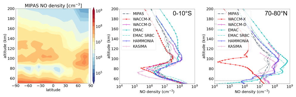
Figure 2 Left: MIPAS zonal mean daily mean daytime NO on 9 January 2010 in the upper mesosphere and thermosphere. Middle and right: MIPAS NO compared against model results from the Snapshot model experiment in 0–10° S and 70–80° N. The error range is the 3σ standard error of the mean. Also shown are results of the SRBC model experiments of EMAC. Note that MIPAS scans to 170 km only, so values above this altitude are dominated by prescribed a priori information.

In low latitudes, observations show a sharp increase of NO into the lower thermosphere with maximal values around 100 km, and a slow decrease with altitude above. All models reproduce the morphology well, but fail to reproduce absolute values; WACCM-X is in good agreement with observations around the lower thermosphere peak in 100–120 km altitude but has significantly lower values above, while all other models overestimate NO compared to observations above 90 km altitude, with highest values at the lower thermospheric peak in HAMMONIA and WACCM-D, and above the peak in EMAC.

At high Northern latitudes, NO shows a broader maximum extending down into the upper mesosphere, indicative of thermosphere-mesosphere coupling in polar winter, and values decreasing with altitude above 110 km. KASIMA, WACCM-D, HAMMONIA, and EMAC qualitatively reproduce this, but show significantly higher values, with highest values shown by EMAC. WACCM-X shows a decrease with altitude from the mesosphere into the lower thermosphere, with a distinct minimum around 90–100 km and a steep increase above. However, WACCM-X values remain lower than the observations or the other models by about one order of magnitude throughout the whole altitude range.

A similar behaviour is observed in comparison with results of the Long model runs extending the comparison over a whole year (see Supplement, Sect. S2.1), indicating that these results might be representative during solar minimum conditions. An additional comparison of results of the Snapshot model experiments against electron densities (as another measure of atmospheric ionization) shows a much narrower range of variability between models, and better agreement with observations than seen for NO (see Fig. S2 in the Supplement, Sect. S2.2). This indicates that the large differences in NO cannot be explained by differences in the ionization forcing. This is especially evident for the comparison of WACCM-X and WACCM-D, which use the same data-sets and parameterizations for the ionization, and the same chemistry scheme, but show very different values of NO around the lower thermosphere peak around 100–120 km altitude in both latitude bands. Differences in either the photochemistry of N(⁴S) and NO above the top of WACCM-D or thermospheric dynamics are therefore more likely the cause than the rate of ionization or the neutral or ion chemistry of the lower thermosphere. This is investigated in the following two sections focussing on WACCM-X and EMAC only, as these models both extend into the mid-thermosphere, above 150 km, but show order-of-magnitude differences in the values of lower thermospheric NO.

3.2 Photochemical formation and loss of N(⁴S), N(²D), and NO

In Fig. 3, NO, N(²D), N(⁴S), and the photochemical lifetime of NO are shown for WACCM-X and EMAC along the 0° meridian at 12:00 UTC on 9 January 2010. The comparison highlights the features already discussed in previous sections: (1) lower NO values in WACCM-X, with a distinct minimum in the Northern high-latitude lower thermosphere and upper mesosphere; (2) higher NO values in EMAC, with a distinct maximum in the polar winter high latitudes extending well into the mesosphere. N(⁴S) and N(²D) show a sharp increase around the mesopause in both models, with values increasing with altitude within the lower thermosphere. Values of N(²D) are of the same order of magnitude. As N(²D) is very short-lived and depends critically on the formation by EUV radiation and particle precipitation (Reactions R1, R2), this indicates again that ionization rates can not be substantially different. N(⁴S) shows a maximum in the mid-thermosphere (140–160 km in WACCM-X, above 160 km in EMAC). Above about 100 km, values of N(⁴S) are much lower in EMAC than in WACCM-X. EMAC values are in much better agreement with results from WACCM-D, HAMMONIA and KASIMA (see Fig. S3 in Sect. S3 of the Supplement for a comparison of all models). The high values of N(⁴S) in WACCM-X have implications for the photochemical lifetime of NO, since the reaction of N(⁴S) with NO (Reaction R15) is the main loss process of NO. Lifetimes of NO considering losses via Reaction (R15), photodissociation and photoionization are shown in the right-hand panels of Fig. 3 and show very low NO lifetimes for WACCM-X in the lower to mid-thermosphere at all latitudes, as well as in the high-latitude polar winter lower thermosphere. Clearly, these losses are anti-correlated with higher values of N(⁴S). The very low values of NO in WACCM-X in the illuminated mid-thermosphere above 140 km as well as in the polar winter lower thermosphere can therefore be explained by larger abundances of N(⁴S) in these altitudes. However, it is not clear why the amount of N(⁴S) is so much higher in WACCM-X than in EMAC. The rates of the main reactions forming N(⁴S) and NO (Reactions R1–R13) are identical or similar for both models with the exception of the partitioning between the formation of N(²D) to N(⁴S) in Reactions (R1) and (R2) (see Table 1), which favours formation of N(²D) over N(⁴S) in WACCM-X, contrary to the observed N(⁴S) surplus. It should also be pointed out that the NO lifetime in the lower thermosphere in WACCM-D agrees much better with EMAC than with WACCM-X, again highlighting that the choice of photochemical and ionic reactions and reaction rates in the lower thermosphere can not be the source of the large discrepancy, which must lie in the mid-thermosphere above the top of WACCM-D.

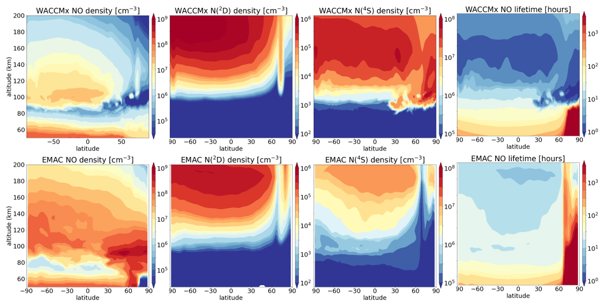
Figure 3 Snapshots of NO (left), N(²D), N(⁴S), and the photochemical lifetime of NO from the Snapshot model experiment on 9 January 2010, 12:00 UTC, at 0° E. Upper panel: WACCM-X, lower panel: EMAC.

Figure 4 Rates of the reactions of (from left to right) N(⁴S) and O₂ (Reaction R3), N(²D) and O₂ (Reaction R4), N(²D) and O and the ratio of atomic to molecular oxygen. Top panels: WACCM-X, bottom panels: EMAC. Snapshot model experiment on 9 January 2010, 12:00 UTC and 0° E.

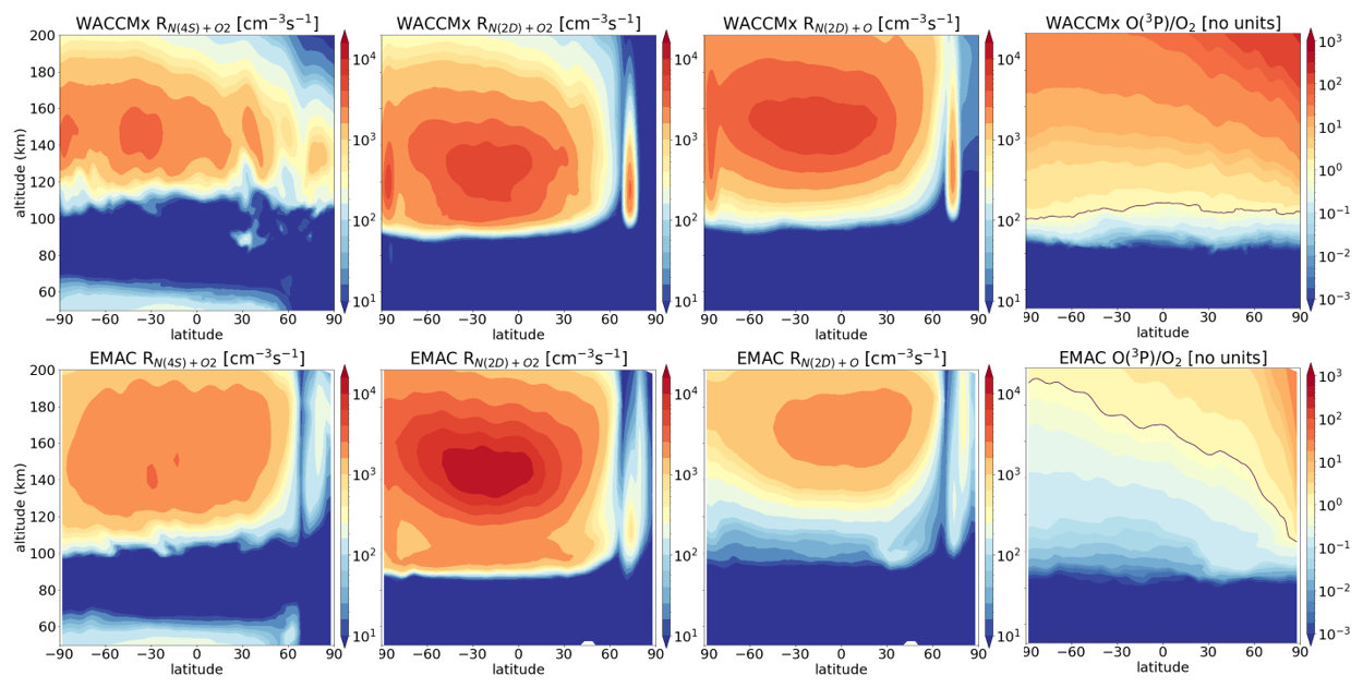
To investigate the reasons for the high amounts of N(⁴S) in WACCM-X further, the rates of two reactions forming NO (Reaction R3: N(⁴S) + O₂, and Reaction R4: N(²D) + O₂) and of the reaction forming N(⁴S) (Reaction R5: N(²D) + O) are shown in Fig. 4. These have been calculated from the results of the Snapshot model experiments of NO, N(⁴S), N(²D), O, O₂ and temperature at 12:00 UTC on 9 January 2010, along the 0° meridian as well as the rate constants used in the respective models. For WACCM-X, the rates of all three reactions fall in a similar range of values, with maximal values of (4000–8000) cm⁻³ s⁻¹ around 120–160 km. In EMAC, the rate of the Reaction (R4) forming NO is distinctly faster than the rates of the other two reactions, and significantly faster than the rate of the same reaction in WACCM-X. The rate of the Reaction (R5) transferring N(²D) to N(⁴S) in EMAC is significantly slower than the rate of the respective reaction in WACCM-X. As the amount of N(²D) is comparable between the two models in the respective altitude ranges, this suggests a significantly different ratio of atomic oxygen to molecular oxygen between WACCM-X and EMAC, with lower values of atomic oxygen and higher values of molecular oxygen, in EMAC.

The ratio of O to O₂ is shown for WACCM-X and EMAC in the right-hand panels of Fig. 4, confirming that this ratio is much lower in EMAC than in WACCM-X. In WACCM-X, the unity line where atomic oxygen equals molecular oxygen is in the lowermost thermosphere around 100 km in all latitudes, while in EMAC, it ranges from above 190 km in the high-latitude Southern hemisphere to around 110 km in the high-latitude Northern hemisphere.

Atomic oxygen in the thermosphere is produced by photodissociation of O₂ in the Schumann-Runge bands, Schumann-Runge continuum, and Lyman-α range as well as by EUV photodissocation of O₂. The rate of EUV photodissociation in all models is based on Solomon and Qian (2005), and therefore should not differ significantly. However, EMAC does not consider photodissociation of O₂ in the Schumann-Runge bands and continuum, while this is included in WACCM-X. The difference in the O to O₂ ratio between WACCM-X and EMAC can therefore presumably be explained by missing photodissociation of O₂ in the Schumann-Runge bands and continuum in EMAC. As the ratio between O and O₂ determines the balance between formation of NO or N(⁴S) by N(²D), this is then also the source of the discrepancy in N(⁴S) between the two models. The amount of N(⁴S), in turn, determines the amount of NO due to its impact on the lifetime of NO.

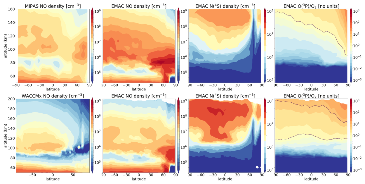
Figure 5 Comparison of (from left to right) densities of NO and N(⁴S) and ratio of atomic to molecular oxygen for the Snapshot and SRBC model experiments of EMAC at 12:00 UTC on 9 January 2010, along the 0° meridian, highlighting the importance of molecular oxygen photodissociation for thermospheric composition. Also shown are MIPAS NO densities (upper left) and WACCM-X NO densities of the Snapshot model experiment on the same day for comparison.

To test this, an additional model experiment was carried out with EMAC including simple parametrizations of O₂ photodissociation in the Schumann-Runge bands and continuum (experiment SRBC). Results from this experiment for NO, N(⁴S) and the ratio of O to O₂ are shown compared to the Snapshot experiment and to MIPAS data and WACCM-X results for 12:00 UTC on 9 January 2010 along the 0° meridian in Fig. 5. It is shown that NO in the thermospheric NO layer decreases significantly when increasing the rate of O₂ photodissociation. When Schumann-Runge bands and continuum are considered, NO in the lower thermosphere is in much better agreement with observations as well as with WACCM-X in the Southern (summer) hemisphere and in low- and mid-latitudes of the Northern (winter) hemisphere. N(⁴S) and the ratio of O to O₂ increase, and are in much better agreement with WACCM-X values for the SRBC case, with the unity line of O to O₂ now around 120 km altitude in EMAC. However, significantly high values of NO compared to observations persist in EMAC in the polar winter lower thermosphere and upper mesosphere, in the same region where NO values in WACCM-X are orders of magnitude lower than observed due to the high abundance of N(⁴S). Though N(⁴S) is formed due to auroral forcing in the high-latitude lower thermosphere via Reaction (R5), the main source region of N(⁴S) in WACCM-X is the low-latitude mid-thermosphere around 150 km altitude (Fig. 4). Therefore, downward-poleward transport in the winter thermosphere might also contribute to the high values of N(⁴S) in the high-latitude lower thermosphere in WACCM-X. This is discussed in the following section.

3.3 Lower thermosphere dynamics and the polar winter lower thermosphere

Atomic oxygen is produced by photodissociation and photoionization of O₂ in the lower thermosphere, and the ratio of O to O₂ increases with increasing altitude, reflecting increasing transition of O₂ to O. As this transition depends on solar illumination, highest values would be expected in the region of strongest illumination, i.e., in the polar summer and tropical regions. However, this is not the case in WACCM-X and EMAC where both show an increase in values of the O to O₂ ratio into polar night in the mid-thermosphere above 150 km (right-hand side panels of Figs. 4 and 5). This suggests downward and poleward transport and mixing from the mid-latitude mid-thermosphere at 140 to 200 km to the high-latitude lower thermosphere below 140 km. Consistent results are derived if the ratio of O to N₂ is considered, which is more commonly used to study as an indicator of vertical motions in the lower thermosphere (see Fig. S4 in Sect. S4 of the Supplement).

Very different scenarios for the meridional motions in the lower to mid thermosphere between WACCM-X and EMAC are indicated by the O to O₂ ratio. For WACCM-X, gradually descending contour lines from the tropical mid-thermosphere to the polar winter lower thermosphere indicate a gradual continuous transport and mixing from the tropical mid-thermosphere to the polar winter lower thermosphere, which efficiently transports N(⁴S) from its main source region in the tropical mid-thermosphere into the polar winter lower thermosphere. The very low values of NO shown in WACCM-X in the polar winter lower thermosphere are therefore likely a combination of strong formation of N(⁴S) from ionizing radiation and N(²D) quenching with O in the tropical and subtropical mid-thermosphere, and downward and poleward transport of N(⁴S) from the source regions to the winter hemisphere lower thermosphere. In EMAC, contour lines of O to O₂ over the winter pole are much steeper than in WACCM-X, and there is a change in the poleward/downward gradient around 60° N. This indicates downward transport mainly over the winter pole, effectively suppressing transport of N(⁴S) from the source region in the mid-and low latitude mid-thermosphere into the polar winter lower thermosphere. Note this change in gradient at the edge of the polar night terminator persists also in the SRBC experiments, and a lack of poleward/downward transport or mixing can explain the persistant high values of NO in the polar winter lower thermosphere in these experiments.

Comparison with NO observations, as discussed in previous sections, indicate that the amount of N(⁴S) in the winter polar lower thermosphere is likely too high in WACCM-X, and too low in EMAC. This suggests that a meridional circulation transporting or mixing NO from the mid-latitude mid-thermosphere to the high-latitude lower thermosphere exists, which is overestimated in WACCM-X, and underestimated in EMAC.

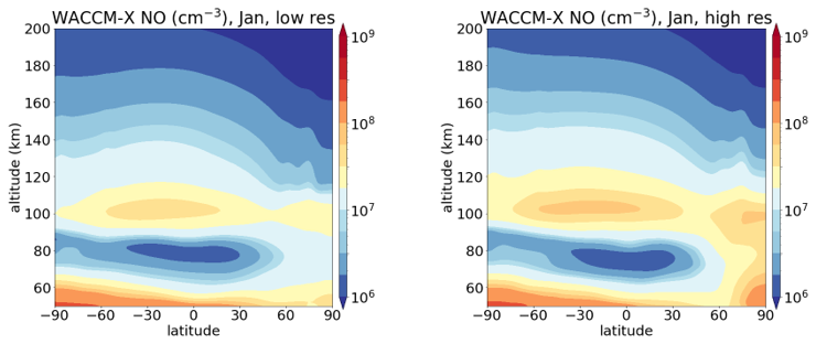
Figure 6 Monthly mean zonal mean January values of NO from two free-running WACCM-X model experiments with moderate (≈ 200 km, left) and high (≈ 25 km, right) resolution under constant moderate solar conditions. The model experiments are described in Liu et al. (2024a). The comparison of polar winter mesospheric and thermospheric NO highlights the impact of model resolution and resolved gravity waves on NO in the lower thermosphere and high-latitude winter lower thermosphere and upper mesosphere.

A comprehensive analysis of the thermospheric circulation and its impact on thermospheric composition is out of the scope of this paper, but in the following, a discussion is provided based on existing model experiments of WACCM-X. Liu et al. (2024a) discuss a possible impact of gravity wave drag in the thermosphere on thermospheric circulation in both the summer and winter hemisphere. They have shown that the thermospheric circulation is better reproduced in WACCM-X in a setup with higher spatial resolution, leading, e.g., to a better representation of the column O to N₂ ratio. Presumably this is because in the model configuration with the higher resolution, a larger part of the gravity wave spectrum is resolved including secondary and tertiary gravity waves forming in the thermosphere (Becker and Vadas, 2020) which are not captured by gravity wave parameterizations. The more realistic representation of thermospheric transport also leads to a better representation of NO particularly in the polar winter lower thermosphere (Fig. 6). The gravity wave parameterization in WACCM-X prevents the propagation of parameterized gravity waves beyond 120 km, while in EMAC, the gravity wave drag is greatly reduced in the thermosphere compared to the mesopause region, but is not totally supressed. Our hypothesis is that there is a thermospheric meridional circulation in the winter hemisphere which is decelerated by gravity wave drag. However, validating this hypothesis is beyond the scope of this paper, and the interplay between thermospheric circulation and composition should be investigated in more detail in the future.

4 Summary and conclusions

Consistent with results of Sinnhuber et al. (2022), we show significant differences in lower thermospheric NO between different chemistry-climate models as well as in comparison to satellite observations. In the low-latitude lower thermosphere, differences are in the range of one order of magnitude, with KASIMA, WACCM-D, HAMMONIA and EMAC showing higher values than observations, while WACCM-X is in range of, or lower than, the observations. In the polar winter lower thermosphere and upper mesosphere, differences reach four to five orders of magnitude between WACCM-X on the one hand, and EMAC, HAMMONIA, WACCM-D and KASIMA on the other hand. The highest values are shown by EMAC, and the MIPAS observations are lower than KASIMA, WACCM-D, HAMMONIA, and EMAC, but significantly higher than WACCM-X. Comparison of electron densities as an indicator of atmospheric ionization shown in Fig. S2, Sect. S2.2 of the Supplement, as well as the large discrepancies between WACCM-X and WACCM-D in the lower thermosphere, indicate that these differences can not be explained by differences in the ionization forcing, photochemistry or ionic chemistry of the lower thermosphere.

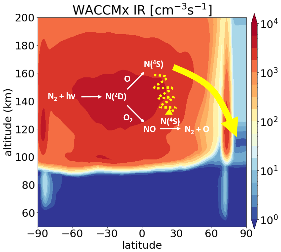
Figure 7 Schematic view of the processes important for NO formation and loss during solar minimum conditions. Dissociation of N₂ by EUV – at high latitudes also energetic particles – leads to the formation of N in the excited states. In the lower thermosphere, N(²D) preferentially reacts with O₂ forming NO, but in the mid-thermosphere, reaction with O dominates forming N(⁴S). In mid- and low latitudes, N(⁴S) is mixed down into the thermospheric NO layer by molecular diffusion (dotted yellow line). In the winter hemisphere, it can also be transported downward and poleward (thick yellow arrow) in a meridional circulation presumably limited by secondary and tertiary gravity waves. Finally, NO is destroyed by reaction with N(⁴S), so the transport and mixing of N(⁴S) from the mid-thermosphere modulates the amount of NO in the lower thermosphere. The underlying figure is the total rate of ionization considering EUV photoionization and particle impact ionization from WACCM-X on 9 January 2010, at 12:00 UT along the 0° meridian.

We find that two processes likely control the amount of NO in the lower thermosphere: (1) The formation of N(⁴S) by photodissociation of N₂ in the illuminated mid-thermosphere, and (2) the downward transport and mixing of N(⁴S) into the NO layer. EUV photodissociation of N₂ produces atomic nitrogen in the ground (N(⁴S)) and excited (N(²D)) state. In the lower thermosphere, N(²D) reacts with O₂ forming NO very efficiently (Reaction R4). In the mid-thermosphere, where atomic oxygen is more abundant than molecular oxygen, the competing reaction of N(²D) with O forming N(⁴S) (Reaction R5) becomes comparatively more important, leading to formation of N(⁴S) in the illuminated mid-thermosphere above 140 km. N(⁴S) is then transported or mixed in a large-scale thermospheric meridional circulation connecting low and high latitudes down into the lower thermosphere and to high latitudes, where its reaction with NO (Reaction R15) is the main loss process of NO. This chain of processes is summarized in Fig. 7.

Our model experiments were carried out for solar minimum conditions, and this has an impact on the rate of formation of NO via Reaction (R3). As this reaction is strongly temperature dependent, higher temperatures in the mid-thermosphere during solar maximum would lead to higher values of NO, and less N(⁴S). Consequently there would be less downward transport of N(⁴S) into the lower thermosphere, and a higher lifetime of NO there. In this sense, the mechanism described above and summarized in Fig. 7 is likely more important during solar minimum conditions. Equally, the low auroral forcing at high latitudes during early 2010 could contribute to the comparatively large impact of the thermospheric meridional circulation on the high-latitude lower thermosphere, as background values of both NO and N(⁴S) are then very low during polar night conditions. In addition the partitioning is likely to favour N(⁴S) during geomagnetically quiet periods, since the formation of N(²D) in the lower thermosphere by continual auroral activity would presumably lead to a larger ambient background of NO, and a higher ratio of NO to N(⁴S).

Sinnhuber et al. (2018)

Table 2 Advantages and disadvantages of model top height for reproducing NO in the polar winter lower thermosphere, a prerequisite of correctly describing the flux of thermospheric NO into the mesosphere and stratosphere during polar winter.

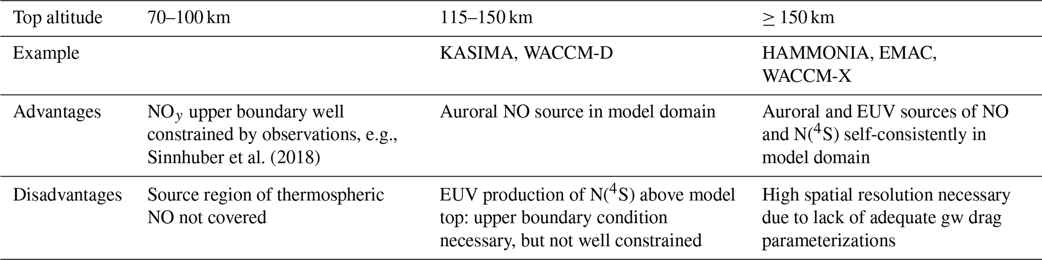
The apparent dependence of lower thermospheric NO on N(⁴S) formed in the middle thermosphere above 140 km altitude means that the model top altitude can have a large impact on how well NO is reproduced in the lower thermosphere, which is a prerequisite to correctly model the amount of thermospheric NO_y transported into the mesosphere and stratosphere during polar winter. Advantages and disadvantages of different model top altitudes can be summarized as follows (see also Table 2):

• For models with their top in or above the mid-thermosphere (HAMMONIA, EMAC, WACCM-X) both a good representation of the rate of O₂ photodissociation and a good representation of thermospheric transport and mixing are necessary for a realistic representation of lower thermospheric NO. This is particularly important for the enhanced NO layer in the polar winter lower thermosphere and upper mesosphere, which appears to depend critically on the downward and poleward transport of N(⁴S) from its source regions in the mid- and low-latitude mid-thermosphere.

• The mid-thermospheric formation of N(⁴S) is missing in models with their top below or near 140 km (WACCM-D, KASIMA). These models need to employ upper boundary conditions of both NO and N(⁴S) to compensate for that. The overestimation of NO in the low- and mid-latitude lower thermosphere in both models could indicate either an underestimation of the upper boundary value for N(⁴S) in these latitudes, or an inefficiency in the downward transport and mixing.

• Models with their top around the mesopause (a very common configuration at the moment) do not cover the lower thermospheric NO layer at all. For these models, an upper boundary condition for NO is necessary. This has been provided, e.g., for CMIP6 (Matthes et al., 2017) based on MIPAS observations (Funke et al., 2016), and at the moment, appears to provide the most realistic representation of the EPP indirect effect (Sinnhuber et al., 2018).

As the meridional circulation in the lower and middle thermosphere in the winter hemisphere appears to be significantly affected by gravity waves, a better representation of the transport of gravity waves across the mesopause as well as the formation of secondary and tertiary gravity waves appears to be necessary to represent NO correctly in the polar winter lower thermosphere and upper mesosphere. This could be achieved, e.g., by models with higher spatial resolution (Becker and Vadas, 2020; Liu et al., 2024a), or by gravity wave drag parameterizations focussing on the thermosphere as described, e.g., in Miyoshi and Yiğit (2019).

Finally, our analysis shows that the interplay between composition and dynamics in the thermosphere is not well understood, and should be a focus of future research.