Identification and quantification of CH₄ emissions from Madrid landfills using airborne imaging spectrometry and greenhouse gas lidar

Methane (CH₄), alongside carbon dioxide (CO₂), is a key driver of anthropogenic climate change. Reducing CH₄ is crucial for short-term climate mitigation. Waste-related activities, such as landfills, are a major CH₄ source, even in developed countries. Atmospheric concentration measurements using remote sensing (RS) offer a powerful way to quantify these emissions. We study waste facilities near Madrid, Spain, where satellite data indicated high CH₄ emissions. For the first time, we combine passive imaging (Methane Airborne Mapper 2D – Light, MAMAP2DL) and active lidar (CO₂ and CH₄ Atmospheric Remote Monitoring – Flugzeug, CHARM-F) remote sensing aboard the German High Altitude and Long Range Research Aircraft (HALO), supported by in situ instruments, to quantify CH₄ emissions. Using the CH₄ column data and European Centre for Medium-Range Weather Forecasts (ECMWF) reanalysis v5 (ERA5) model wind information validated by airborne measurements, we estimate landfill emissions through a cross-sectional mass balance approach. Strong emission plumes are traced up to 20 km downwind on 4 August 2022, with the highest CH₄ column anomalies observed over active landfill areas in the vicinity of Madrid, Spain. Total emissions are estimated to be up to ∼ 13 t h⁻¹. Single co-located plume crossings from both instruments agree well within 1.2 t h⁻¹ (or 13 %). Flux errors range from ∼ 25 % to 40 %, mainly due to boundary layer (BL) and wind speed variability. This case study not only showcases the capabilities of applying a simple but fast cross-sectional mass balance approach, along with its limitations due to challenging atmospheric boundary layer conditions, but also demonstrates, to our knowledge, the first successful use of both active and passive airborne remote sensing to quantify methane emissions from hotspots and independently verify their emissions.

1 Introduction

Methane (CH₄) is the second most important anthropogenic greenhouse gas after carbon dioxide (CO₂). It has an effective radiative forcing of ∼ 0.54 W m⁻¹, or one-quarter of that of CO₂ (Forster et al., 2021). It is a more potent greenhouse gas than CO₂ by a factor of 81 per unit mass on a time horizon of 20 years (Forster et al., 2021), and its atmospheric lifetime, which is dominated by the oxidation agent hydroxyl (OH) and transport and oxidation in the stratosphere, is relatively short (∼ 12 years; Szopa et al., 2021). For the above reasons, Shindell et al. (2012) proposed that the reduction in CH₄ emissions was a potentially valuable short-term strategy to reduce the impact of anthropogenic emissions on the climate. This objective became part of international environmental policy through the Global Methane Pledge, an initiative launched by the European Union (EU) and the United States (US) with the goal of reducing anthropogenic CH₄ emissions by 30 % from 2020 to 2030 (EU-US, 2021).

Landfills and waste-related activities are estimated to account for one-fifth of anthropogenic CH₄ emissions (Saunois et al., 2020). Within landfills, CH₄ (but also CO₂ and other gases, such as precursors of short-lived climate pollutants and greenhouse gases, such as non-methane hydrocarbons) are produced by anaerobic decomposition of organic matter by microbes (e.g. Eklund et al., 1998). This methane has been and is released to the atmosphere nearly unhindered from unmanaged landfills. Alternatively, in the context of greenhouse gas mitigation, measures exist to reduce these emissions, e.g. by installing gas collection systems to recover a large fraction of the CH₄ (e.g. Parameswaran et al., 2023) for possible energy generation in gas-fired power plants or flaring, and/or by deploying special covers, which partly oxidize CH₄ to the less potent greenhouse gas CO₂ (e.g. Bogner et al., 1997). Despite these management strategies, mitigation and reduction efforts, which are typically only available in the developed world (Kumar et al., 2023; Kaza et al., 2018), reported CH₄ emissions from waste (IPCC sector 5) are 97 Mt CO_2,eq yr⁻¹ (or 3.5 Mt yr⁻¹)¹ and still account for ∼ 24 % (or ∼ 18 % if only solid waste disposal, IPCC sector 5A, is considered) of the anthropogenic CH₄ emissions in the European Union in 2022 (EEA, 2024).

Of relevance to this study, Tu et al. (2022) investigated landfill sites and related facilities in Madrid, Spain. There, significant amounts of CH₄ have been identified to be released to the atmosphere. Based on satellite observations, acquired between May 2018 and December 2020, Tu et al. (2022) suggest an underestimation in the reported emissions by the European Pollutant Release and Transfer Register (E-PRTR; EEA, 2024) by a factor of ∼ 3. Their estimated emissions would correspond to ∼ 4 %² of Spain's national CH₄ emissions in 2020 reported to the United Nations Framework Convention on Climate Change (UNFCCC; EEA, 2023).

Landfill facility emissions must be reported to the authorities (E-PRTR) in the European Union to comply with the objectives of EU directives if they meet certain criteria, such as emitting more than 100 t CH₄ yr⁻¹, receiving more than 10 t d⁻¹, or having a total capacity of more than 25 kt (European-Parliament, 2006). This reporting is usually carried out using bottom-up estimates of methane emissions described in IPCC (2006, 2019). However, emissions based on these bottom-up estimates may be underestimated due to inaccurate model parameters (Wang et al., 2024) and often differ from those using atmospheric measurements (top-down, e.g. Lu et al., 2022; Maasakkers et al., 2022; Duren et al., 2019).

In the past, different approaches have been used from different platforms to provide independent validation of waste facility emissions. Commonly used measurement techniques are ground-based measurements of the gases by closure chambers, scattered across the landfill surface (e.g. Xie et al., 2022; Jeong et al., 2019; Trapani et al., 2013), greenhouse gas in situ analyser measurements downwind of landfills with (e.g. Monster et al., 2014a, b) and without (e.g. Liu et al., 2023; Xia et al., 2023) tracer, and vertical or horizontal scanning lidar observations (e.g. Innocenti et al., 2017; Zhu et al., 2013) or Fourier-transform infrared (FTIR) spectrometer measurements (Sonderfeld et al., 2017). Another strategy involves airborne (e.g. Ren et al., 2018; Krautwurst et al., 2017; Cambaliza et al., 2015, 2014; Peischl et al., 2013; Mays et al., 2009) or drone (Fosco et al., 2024, and references therein) observations collecting in situ CH₄ concentrations downwind of a landfill. Comprehensive comparisons of these techniques are given by Mønster et al. (2019) and Babilotte et al. (2010). Recently, passive remote sensing (RS) imaging instruments exploiting solar electromagnetic radiation in the near- and short wave infrared have been deployed, which map CH₄ column amounts of the plumes leaving a landfill (e.g. Cusworth et al., 2024, 2020) in addition to airborne thermal imagers (e.g. Tratt et al., 2014). These allow not only precise leakage detection, but also emission quantification. Moreover, nowadays, high-spatial-resolution (in the order of several tens of metres) satellite instruments are exploited in terms of CH₄ column observations for a more regular investigation of landfills (e.g. McLinden et al., 2024; Maasakkers et al., 2022) than was possible with irregular campaign deployments in the past. However, satellite observations with a coarse spatial resolution of some kilometres were also used to constrain landfill emissions (e.g. Balasus et al., 2024; Nesser et al., 2024) but not to the same level of detail as their high-spatial-resolution counterparts.

Besides the predominately passive remote sensing approaches mentioned, there is currently no satellite mission using active CH₄ remote sensing in orbit, and we are not aware of any studies utilizing active airborne remote sensing to measure landfill emissions. Notably, Amediek et al. (2017) quantified local CH₄ emissions from coal mine ventilation shafts, demonstrating the capabilities of active airborne remote sensing measurements for such endeavours. Active remote sensing instruments are independent of sunlight because they use a laser as their own source of electromagnetic radiation. In contrast to airborne and satellite-borne passive instruments, they can measure during the day and night across all seasons and latitudes. They provide ranging capabilities resulting from the precise measurement of the propagation time of the emitted light and, due to their narrow field of view, measure between clouds. Integrated path differential absorption (IPDA) lidars potentially provide highly accurate measurements without varying biases: the exceptions are those introduced by small differences in the scattering and reflectivity of the ground scene and any inaccuracies in the knowledge of the absorption cross-sections. However, Wolff et al. (2021) showed that, under turbulent conditions, the spatial distribution of enhanced concentrations within an exhaust plume may be highly heterogeneous. As a result, a single overflight may sample sections with stronger or weaker enhancements purely as a result of the local variability. In some cases, the true emission signal only emerges after averaging over a high number of overflights.

To account for this potential limitation, in the analysis, we combine active lidar with passive imaging spectrometry, both designed to capture atmospheric CH₄ column gradients. Thus, we obtain both high-precision transects and spatial context, which supports a more robust interpretation of the observed CH₄ column enhancements. Moreover, these remote sensing measurements are complemented by auxiliary in situ measurements of CH₄, CO₂, and 3D winds in support of the remote sensing data. It was the first time that this payload was flown aboard the same aircraft acquiring spatially and temporally co-located active and passive remote sensing measurements side by side for the acquisition of atmospheric CH₄ column observations. The greenhouse gas lidar CO₂ and CH₄ Atmospheric Remote Monitoring – Flugzeug (CHARM-F) is an airborne demonstrator for the future satellite mission, MEthane Remote Sensing LIdar missioN (MERLIN; Ehret et al., 2017). The passive-imaging Methane Airborne Mapper 2D – Light (MAMAP2DL) remote sensing instrument demonstrates the applicability of the CH₄ proxy retrieval (see below) at scales probed by Copernicus Anthropogenic Carbon Dioxide Monitoring (CO2M; Sierk et al., 2021) and the Twin Anthropogenic Greenhouse Gas Observer (TANGO; SRON, 2024). The observations were collected in 2022 as part of the Carbon Dioxide and Methane (CoMet 2.0) Arctic mission in Canada (CoMet, 2022). Prior to the transfer to Canada, an initial research flight was carried out to test all the instruments. This test flight was performed on 4 August over Madrid to investigate the unexpectedly high landfill emission rates reported by Tu et al. (2022) and in a webstory from the European Space Agency (ESA) from October 2021 (ESA, 2021).

In Sect. 2, we provide a brief summary of the CoMet 2.0 mission and introduce the main instruments MAMAP2DL and CHARM-F used in this study (Sect. 2.1). This also includes a description of the algorithms used to infer CH₄ columns from the measurements (Sect. 2.2); additional steps necessary to achieve comparability between the passive and active observations (Sect. 2.3); and the cross-sectional flux method, which is used to quantify the CH₄ emissions (Sect. 2.4). Section 3 describes the observed CH₄ plumes over Madrid from both remote sensing instruments. These data are used to pinpoint the exact source locations within the landfill area (Sect. 3.1), followed by a rigorous comparison of the active and passive data (Sect. 3.2), a comparison of the resulting emission fluxes (Sect. 3.3), and a comprehensive discussion of potential uncertainties (Sect. 3.4). We close the paper by discussing our fluxes in a broader context (Sect. 4) and summarizing our findings (Sect. 5).

2 Methods and data

2.1 Campaign and instrumentation

Below we describe the waste treatment facilities that were the targets of the research flights and the flight strategy used to derive their methane emission rates. We then describe the instruments used, which were installed aboard the German High Altitude and Long Range Research Aircraft (HALO), operated by the Deutsches Zentrum für Luft- und Raumfahrt (DLR), type: Gulfstream G550. The retrieval algorithms used to derive the CH₄ columns are explained next. This is followed by a description of the observed CH₄ columns. Finally, we derive the methane fluxes, i.e. the methane emission rates, using the plume cross-sections.

2.1.1 Target description and flight strategy

The targets under consideration were the Mancomunidad del Sur landfill in the Pinto municipality (40.264° N, 3.633° W; hereafter: Pinto landfill) and the Valdemingómez Technology Park (VTP; 40.332° N, 3.586° W) in the southeast of Madrid, Spain. The latter is a waste treatment complex that accepts around 1222 kt (Madrid, 2022) of waste, of which around 140 kt was deposited at the Las Dehesas landfill site in 2022 (Spanish-PRTR, 2025a), and houses several waste treatment facilities including the largest biomethane plant in Spain (Calero et al., 2023), which is also one of the largest in Europe (UABIO, 2022). Additionally, it contains landfill sites such as the non-operating Valdemingómez landfill (40.331° N, 3.580° W) equipped with a gas recovery system and an active landfill site (40.325° N, 3.591° W; hereafter: Las Dehesas landfill) next to the waste treatment plant Las Dehesas. The northern half of the Las Dehesas landfill, where certain areas (i.e. cells) are already full and therefore closed, are also equipped with a gas recovery system (Sánchez et al., 2019). The two landfills in the technology park are spread over an area of ∼ 0.9 and 0.6 km² for the inactive Valdemingómez site and the active Las Dehesas site, respectively. More details about the different facilities are in the Annual Report for 2022 for the VTP (Madrid, 2022). The Pinto landfill, further to the south, stretches over ∼ 1.5 km². It opened in 1987 and is still operational, with around 53 kt of waste being dumped in 2022 (Spanish-PRTR, 2025b), and the already closed parts of the landfills are equipped with a gas recovery system (MdS, 2024). The topography around these landfill sites shows some variability, ranging from about 550 to 700 $\mathrm{m}\mathrm{a}.\mathrm{g}.\mathrm{l}.$ (above ground level) with a small valley between the two sites and a steep rise just south of the VTP, according to Google Earth.

According to the Spanish PRTR (Spanish-PRTR, 2025c), the combined annual reported 2022 CH₄ emissions for the two facilities “Vertresa-Urbaser, S.A. UTE (UTE Las Dehesas)”³ and “Deposito controlado de residuos urbanos de Pinto”⁴ are 0.2 t h⁻¹. Both sites are classified as “landfills” according to the European-Parliament-Annex (2006, Regulation (EC) 166/2006 E-PRTR, Annex I). We assume that these reported values are representative for the two investigated areas, which include landfills and waste treatment plants, as other listed sources would not contribute significantly to the emissions according to the Spanish PRTR (Spanish-PRTR, 2025c). According to the European-Commission (2006), both landfills appear not to use strict IPCC reporting methods. They report the methods “OTH” (for other measurement or calculation methodology) and “C” (for calculation) using “issue factors” and the methods “CRM” (for measurement methodology by means of certified reference materials) and “M” (for measurement) using “electrochemical cells” for the Las Dehesas and Pinto landfills, respectively, in 2022. In addition, the reporting method for the Pinto landfill changed from 2021 to 2022, while “OTH” and “C” using “an American EPA (Environmental Protection Agency) calculation model” was applied in 2021 instead of CRM as in 2022.

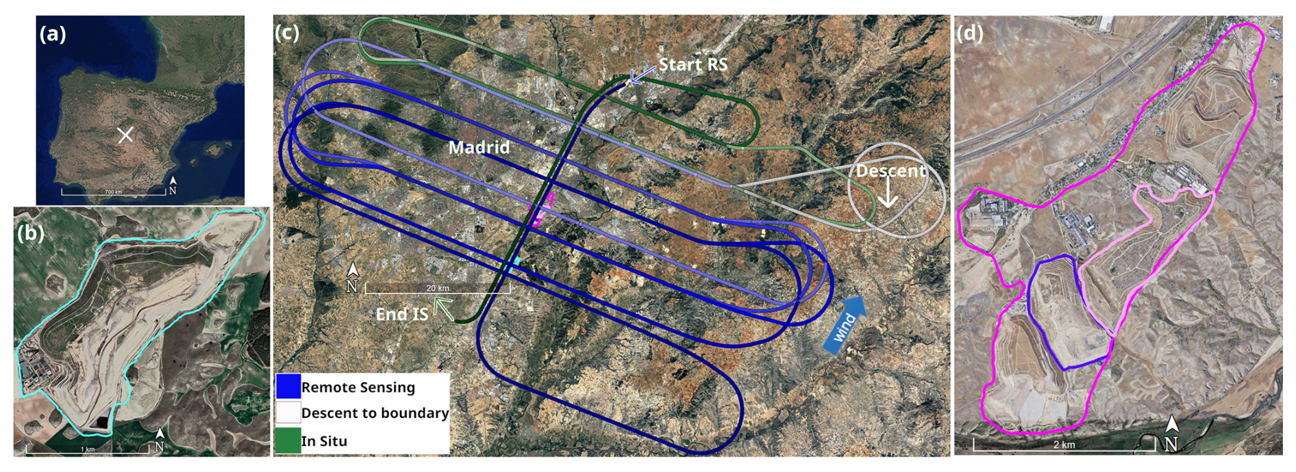
Figure 1 Top view of the flight path of HALO during the test flight over Madrid. An overview map in Google Earth of the Iberian Peninsula is shown in panel (a), and Madrid is marked by the white cross. Panel (b) shows a zoom-in of the Pinto landfill, outlined with a solid cyan line. Panel (d) displays the Valdemingómez Technology Park (VTP), marked with a solid magenta line. In the same panel, the closed Valdemingómez landfill is shown in pink, and the open Las Dehesas landfill is highlighted in purple. The flight path is shown in panel (c), whereby bluish colours represent the remote sensing (RS) part at ∼ 7.7 $\mathrm{km}\mathrm{a}.\mathrm{g}.\mathrm{l}.$ and greenish colours represent the in situ (IS) part at ∼ 1.6 $\mathrm{km}\mathrm{a}.\mathrm{g}.\mathrm{l}.$ (above ground level) of the flight. For better visualization, the greenish in situ part is slightly shifted to the northwest; otherwise, part of the legs would be hidden by RS legs. The map underneath is provided by © Google Earth, using imagery by Landsat/Copernicus, Maxar Technologies.

To properly investigate emissions from these two landfills, dedicated flight patterns where the aircraft is levelled (so-called flight legs) were aligned perpendicular to the forecasted wind direction (Fig. 1). The overflight time was between 13:00 and 15:40 local time (11:00 to 13:40 UTC) on 4 August 2022. This time window was chosen using knowledge of the weather forecast predicting stable winds around noon, which also favoured the observations by the passive remote sensing instrument due to the high position of the sun.

Prevailing wind direction during the flight was from approximately SSW, aligned with the two waste treatment areas (Fig. D2 in Appendix D1 shows time-resolved wind profiles for the time measured in the measurement area). For later emission rate estimates (Sect. 2.4), flight legs were mostly flown perpendicular to the mean wind direction at several distances downwind from the sources at altitudes of ∼ 7.7 and 1.6 $\mathrm{km}\mathrm{a}.\mathrm{g}.\mathrm{l}.$ (above ground level), as depicted in Fig. 1. The higher flight altitudes were flown to optimize passive and active remote sensing observations, whereas the lower altitudes were used to primarily collect in situ observations within the boundary layer (BL) inside and outside of the emission plumes, along with high-spatial-resolution CH₄ imaging data. Remote sensing observations were collected upwind of each of the landfills to account for potential inflow of CH₄ and to separate emissions from the two waste treatment areas.

Moreover, the flight pattern started with one straight leg against the wind direction directly overflying the landfills at remote sensing altitude at ∼ 7.7 $\mathrm{km}\mathrm{a}.\mathrm{g}.\mathrm{l}.$ to identify emission hotspots using the imaging capabilities of MAMAP2DL. Then, perpendicular remote sensing legs were flown in an alternating order due to the large turning radius of the aircraft. Three legs were repeated twice. Afterwards, the aircraft descended to the altitudes optimal for in situ measurements, flying four legs downwind of both areas. Lastly, the flight pattern was closed with a straight leg overflying both landfills directly at in situ altitude. The in situ flight was performed after the remote sensing part towards the afternoon, when a fully developed BL favours these measurements.

2.1.2 Passive MAMAP2DL remote sensing imaging instrument

Methane Airborne Mapper 2D – Light (MAMAP2DL) is a lightweight airborne imaging greenhouse gas sensor for mapping atmospheric column concentration anomalies of CH₄ and CO₂ (in $\mathrm{molec}.{\mathrm{cm}}^{-\mathrm{2}}$ or in % relative to the given background column). It builds on the heritage of MAMAP (Gerilowski et al., 2011) and is a passive remote sensing instrument which collects backscattered solar radiation mainly from the ground which has been modified by absorption from atmospheric gases. Using absorption spectroscopy, the depth of these absorption lines is interpreted as column gas concentrations in the atmosphere (for details, see Sect. 2.2.1). MAMAP2DL comprises a grating spectrometer and records spectra in the range between 1558 and 1689 nm, where prominent absorption features of CH₄ and CO₂ exist (Krings et al., 2011), having a spectral resolution of around 1 nm with a spectral sampling of ∼ 3 to 4 pixels per full width at half maximum (FWHM). The front optics map the measurement scene via 28 optical fibres onto a 2D sensor consisting of 384 pixels in the horizontal direction and 288 pixels in the vertical direction. The horizontal direction maps onto the spectral axis, and the vertical direction maps onto the spatial axis (see also Fig. 2). Each optical fibre is mapped onto around six usable lines on the chip which are binned to increase the signal-to-noise ratio before further analysis. For the Madrid flight, the exposure time for a single readout was between 40 and 45 ms. This would result in a ground scene size of ∼ 110 × 8.5 m² (across × along-flight direction). To achieve quadratic ground scenes, we therefore bin 13 ground scenes in along-flight direction after the retrieval of the column anomalies.

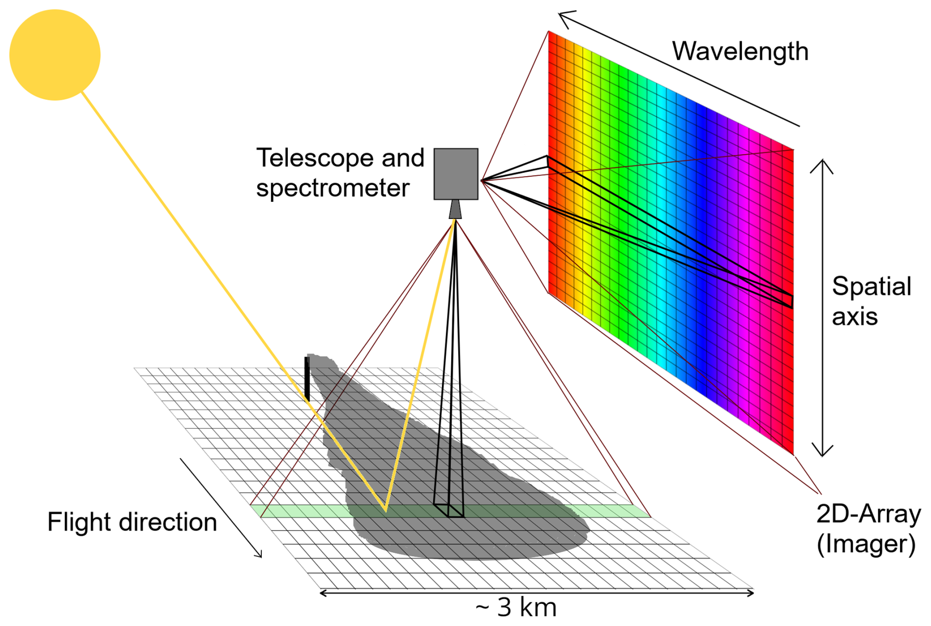
Figure 2 The schematic diagram shows the measurement principle of MAMAP2DL. The instrument simultaneously acquires 28 ground scenes across track with a swath width of ∼ 3 km at a flight altitude of ∼ 7.7 $\mathrm{km}\mathrm{a}.\mathrm{g}.\mathrm{l}$. The final ground scene size is ∼ 110 × 110 m².

The instrument was built at the Institute of Environmental Physics (IUP) at the University of Bremen (UB), and its design has its heritage in the non-imaging greenhouse gas sensor MAMAP (Gerilowski et al., 2011) built at IUP UB in 2006. MAMAP2DL shares many of the optical concepts developed in MAMAP but uses a spectrometer consisting of lenses instead of mirrors and a 2D detector array allowing the imaging of emission plumes. MAMAP’s column observations have been proven to be of high data quality, achieving a single-measurement precision of ∼ 0.2 % for the background-normalized column anomaly (Krautwurst et al., 2021). Its observations have been used successfully to estimate CO₂ emissions from single power plants (Krings et al., 2011) and power plant clusters (Krings et al., 2018) and were part of a model validation study for power plant emissions (Brunner et al., 2023). CH₄ emissions from coal mine ventilation shafts (Krautwurst et al., 2021; Krings et al., 2013) and landfills (Krautwurst et al., 2017) were determined, and upper limits of emissions from offshore geological CH₄ seeps (Krings et al., 2017; Gerilowski et al., 2015) were estimated.

2.1.3 Active CHARM-F remote sensing instrument

CO₂ and CH₄ Remote Monitoring – Flugzeug (CHARM-F), developed and operated by DLR, is an IPDA lidar instrument that consists of a pulsed laser transmitter and a receiver system. The transmitter is based on two optical parametric oscillators (OPOs) which are pumped by means of diode-pumped, injection-seeded, and Q-switched Nd:YAG lasers in a master oscillator power amplifier configuration. Installed on an aircraft, the nadir-oriented lidar emits laser pulses at two precisely tuned wavelengths in the near-infrared (NIR) at ∼ 1645 nm for CH₄ and ∼ 1572 nm for CO₂. These two laser pulses propagate through the atmosphere until they are backscattered at a surface. From the backscattered intensities entering the detector, absolute column-averaged mixing ratios of carbon dioxide (XCO₂ in ppm) and methane (XCH₄ in ppb) below the aircraft are derived (see Amediek et al., 2017, and Appendix C1). A schematic illustration of the IPDA measurement principle is shown in Fig. 3.

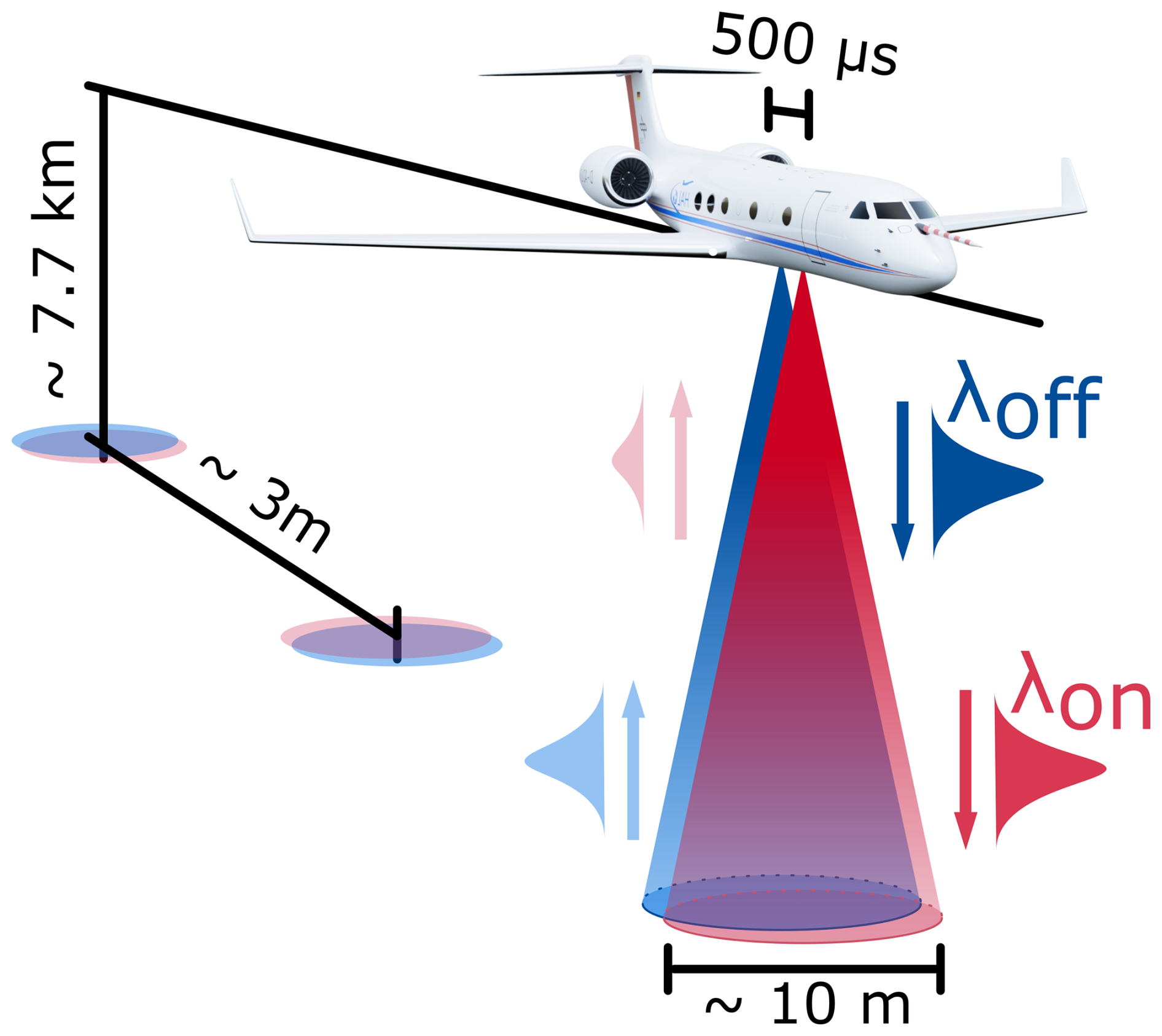
Figure 3 The measurement geometry of CHARM-F installed on HALO. Two laser pulses are emitted towards the Earth with a delay of 500 µs. The laser pulse with the online wavelength is denoted as λ_on, while the one with the offline wavelength is denoted as λ_off. The concentration in the surveyed column can be derived from the backscattered intensities. As the footprints are larger than the distance between consecutive pulse pairs, they actually overlap. For the visualization above, they were pulled apart. The order in which the on–off pairs are sent out alternates.

The generation of narrow-band wavelength is realized by injection-seeding the OPOs with continuous wave (CW) radiation from stabilized distributed feedback (DFB) lasers. In order to fulfil the stringent requirements on frequency stability for the online and offline wavelengths, a sophisticated locking scheme was developed, based on DFB lasers referenced to a multi-pass absorption cell and offset locking techniques (Amediek et al., 2017; Quatrevalet et al., 2010). The online and offline laser pulses are emitted as double pulses with a temporal separation of 500 µs and a repetition rate of 50 Hz.

CHARM-F's receiving system consists of four receiving telescopes, two for each greenhouse gas, with a diameter of 20 and 6 cm and equipped with InGaAs pin diodes and InGaAs avalanche photo diodes (APDs), respectively. This redundant measurement capacity proved to be very valuable for an independent quality assessment of the data. The received signals are sampled using fast digitizers and are processed by means of a home-built data acquisition system. Two digital cameras (in the visible light spectrum (VIS) and NIR spectral range) provide additional context information of the ground scene.

In the context of this study, we only make use of the XCH₄ measurement, which is fully independent of the CO₂ channels. The CH₄ wavelengths, at which CHARM-F operates, are at 1645.55 and 1645.86 nm for online and offline wavelengths, respectively.

Previous work has shown that CHARM-F measurements are suitable for quantifying CH₄ and CO₂ emission sources (Amediek et al., 2017; Wolff et al., 2021). Furthermore, CHARM-F serves as a technology demonstrator for the MERLIN space-borne methane lidar that will measure methane columns globally starting in the late 2020s (Ehret et al., 2017).

2.1.4 Auxiliary data

In support of the remote sensing data, we use additional measurements from in situ instruments aboard HALO and model data. To adapt radiative transfer model (RTM) simulations used later during the retrieval process of MAMAP2DL data (for details, see Sect. 2.2.1) to prevailing atmospheric background conditions, we use CH₄ and CO₂ in situ observations from JIG (operated by Max-Planck-Institute for Biogeochemistry, MPI-BGC; Gałkowski et al., 2021; Chen et al., 2010) and H₂O from the BAHAMAS suite (Giez et al., 2023), recorded at frequencies of 1 Hz (CH₄), 1 Hz (CO₂), and 10 Hz (H₂O). CH₄ and CO₂ are measured with a precision and accuracy of 1 and 2 ppb and 0.1 and 0.2 ppm, respectively. Measurements of H₂O have an uncertainty of up to ∼ 5 %. Furthermore, for the correct georeferencing of the remote sensing observations, positioning and attitude data of HALO also measured by the BAHAMAS suite at 10 Hz are used.

A critical parameter for the flux and emission rate calculation is the wind in the BL, where the exhaust plumes are located. The BAHAMAS system delivers highly accurate in situ wind measurements at 10 Hz. The uncertainty of the horizontal wind speed and direction is usually ∼ 0.14 m s⁻¹ and ∼ 2.9°, respectively, for low flying altitudes (Giez et al., 2023). A special data analysis for the Madrid flight shows slightly increased errors due to the replacement of the static pressure sensor and the strong turbulence, but the wind measurements are still of very high quality with uncertainties of ∼ 0.2 m s⁻¹ and ∼ 4° for the relevant altitude levels.

During the remote sensing measurements, the wind information within the BL is needed but is not measured, as HALO was flying well above at ∼ 7.7 $\mathrm{km}\mathrm{a}.\mathrm{g}.\mathrm{l}$. Therefore, we use the wind measurements from the BAHAMAS system to verify the quality of the European Centre for Medium-Range Weather Forecasts (ECWMF) reanalysis v5 (ERA5) model (Hersbach et al., 2020) in that area on that day. We use ERA5 data with a temporal and horizontal spatial resolution of 1 h and 31 km, respectively, and 137 altitude levels. The comparison is found in Appendix D1 and shows a very good agreement between measurements and model, with averaged deviations of 0.05 m s⁻¹ and 0.8° within the BL, and thus gives confidence for the use of the ERA5 winds in our study.

We also use airborne in situ observations to validate the boundary layer height (BLH) from ERA5. The analysis is given in Appendix D2 and reveals that the observed boundary layer heights during the flight are up to 15 % lower than those given in ERA5.

2.2 Retrieval algorithms

The following subsections describe how atmospheric columns are derived from the measured spectra in the case of the passive instrument and from the backscattered laser pulses in the case of the active instrument.

2.2.1 CH₄ column anomalies by MAMAP2DL

For the analysis of the MAMAP2DL spectral data, the weighting function modified differential optical absorption spectroscopy (WFM-DOAS) approach is used. It was originally developed for the spaceborne instrument SCIAMACHY aboard ENVISAT (Buchwitz et al., 2000) and was later adapted to airborne geometry for the MAMAP sensor (Krings et al., 2011). The latest version of the algorithm is described in Krautwurst et al. (2021) and has been applied to the imaging data from MAMAP2DL. The results are background-normalized column anomaly maps of CH₄ or just CH₄ column anomalies.

For the current study, the single measurement precision of the CH₄ column anomalies, derived from MAMAP2DL columns in areas not (or only a little) influenced by emissions, is around 0.4 % (1σ) for ∼ 110 × 110 m² ground scenes. The accuracy of the CH₄ column anomalies is estimated to be around 0.14 %, possibly not correctable by the applied normalization processes. Further details about the algorithm setup and uncertainties associated with it are given in Appendix B.

The retrieved anomaly maps are also orthorectified (also known as georeferencing). A correction is applied along the lines, as described in Schoenhardt et al. (2015), to account for the orientation of the aircraft (e.g. pitch, roll, yaw), which would lead to spatially incorrectly projected ground scenes and would prohibit proper source allocation. For that, attitude data provided by the BAHAMAS system at 10 Hz resolution have been used. Visual inspection of measured intensity maps overlaid on Google Earth yields a relative accuracy to Google Earth imagery of ∼ 110 m (or approx. one MAMAP2DL ground scene; see Appendix B4 for details).

2.2.2 XCH₄ by CHARM-F

IPDA lidars, such as CHARM-F, directly measure the differential absorption optical depth (DAOD) between the online and offline wavelength from backscattered signals without the need for auxiliary information. The DAOD is converted into a weighted column average of the dry-air molar mixing ratio of the trace gas in question by applying the so-called weighting function (see Appendix C1).

The weighting function depends, apart from precise spectral information, also on external information about the state of the atmosphere below the aircraft, such as temperature, pressure, and humidity, vertically resolved. For spectroscopic reasons, the sensitivity of CHARM-F for methane is highest close to the ground but varies by only a few percent within the lower troposphere (Ehret et al., 2008, 2017).

As mentioned in Sect. 2.1.3, CHARM-F is equipped with two detector channels for CH₄. For this study, XCH₄ measurements from both detectors are combined in a weighted average, where the inverse variance due to noise is used as weights.

For the conditions present during the Madrid measurements, the statistical uncertainty (1σ error) of a single XCH₄ measurement (averaging both available detectors), based on one online pulse and one offline pulse, is on the order of 5 %. The main contributing random sources of error are shot and detector noise, along with random variations in the speckle and albedo pattern (Ehret et al., 2008).

When averaging along the flight track over multiple double-pulse measurements, this uncertainty decreases, as expected, by 1 over the square root of the number of measurements, until systematic drifts and offsets start to dominate. For the 3 s averaging, which corresponds to a distance of about 500 m on the ground and which is used in the plots, visualizations, and flux computations that are shown in the following, the statistical measurement uncertainty is roughly 10 ppb or 0.5 %.

Due to the background normalization that is performed as part of the flux calculation conducted in this context, the results are largely unaffected by constant offsets and slow drifts in the methane column. Our conversion into total columns and comparison with predicted values from the Copernicus Atmosphere Monitoring Service (CAMS) global inversion model (CAMS, 2023) suggest an offset of less than 0.5 %. See Appendix C3 for more details.

2.3 Common columns

In order to allow a better comparison between active and passive remote sensing measurements and the application of a uniform approach for computing cross-sectional fluxes with both instruments, CHARM-F partial columns (PCs; below the aircraft) XCH₄ have been converted into total-column (TC) relative enhancements (column anomalies). This conversion requires assumptions about the composition and structure of the atmosphere that are not directly accessible from CHARM-F measurements alone. A detailed formalized description of this conversion can be found in Appendix C2.

In order to estimate a relative column anomaly, the methane concentration from the CAMS global inversion model (CAMS, 2023) is used as a reference. For the partial column between the aircraft and the ground, XCH₄ measured by CHARM-F is compared to the corresponding value calculated based on CAMS and the CHARM-F weighting function. For the partial column above the aircraft, the anomaly is zero by definition.

For the partial column below the aircraft, a small correction (corresponding to a 2 %–3 % relative scaling effect on the column anomaly) for the effect of the weighting function has to be applied to the column anomaly computed using CHARM-F measurements. As explained in Sect. 2.2.2, due to the spectroscopic properties of methane and the choice of lidar wavelengths, CHARM-F is somewhat more sensitive close to the ground than in the upper troposphere. As a correction factor for the anomaly of the partial column, we use the ratio between the average weighting function for the full column below the aircraft and the average column only within the BL. This assumes that methane emitted from the landfills is only dispersed within the BL.⁵

Finally, the anomalies of the partial columns above and below the aircraft are combined in a weighted average with the number density of (vertically summed) air molecules per area as weights.

2.4 Flux computation

Already during the planning activities for the Madrid flight (see Sect. 2.1.1), the position and orientation of the flight legs were designed for the application of a cross-sectional mass balance approach or flux method. To account for instrument-specific properties, two slightly different methods are applied and described in the following. Both follow the widely applied approach for in situ (Klausner et al., 2020; Peischl et al., 2018; Cambaliza et al., 2015; Lavoie et al., 2015) or remote sensing (Fuentes Andrade et al., 2024; Wolff et al., 2021; Reuter et al., 2019; Krings et al., 2018; Varon et al., 2018; Frankenberg et al., 2016) observations, where the mass of molecules that is transported through an imaginary curtain or cross-section is computed by

$$\begin{array}{}\text{(1)}& F_{\mathrm{cs}}=f\cdot \sum _i\mathrm{\Delta }{V}_i\cdot \mathrm{\Delta }{x}_i\cdot u_i\cdot \cos \left({\mathit{\alpha }}_i\right),\end{array}$$

where F_cs is the resultant and areal-integrated CH₄ mass flux or the CH₄ mass flow rate in t hr⁻¹ of one cross-section. In the following, we use the term “flux” when talking about mass flow rates through a cross-section, and we use “emission rate” if the flux is attributed to a certain source or source area. f is a conversion factor⁶ to transform to units of t hr⁻¹, ΔV_i is the retrieved CH₄ column anomaly in $\mathrm{molec}.{\mathrm{cm}}^{-\mathrm{2}}$, Δx_i is the valid length element for the corresponding ΔV_i in metres, u_i is the absolute wind speed (or effective wind speed valid for the plume) in m s⁻¹, and α_i is the angle between the normal of the length element and the wind direction in degrees to calculate the wind fraction perpendicular to the length element. The sum indicates the summation over all observations i within the plume.

The first modification of Eq. (1) accounts for the characteristics of the imaging data from the MAMAP2DL sensor. The retrieved CH₄ anomaly maps consist of strips with a swath width of ∼ 3 km and 28 ground scenes across track (see Fig. 2), which are, however, additionally distorted by the movement of the aircraft (see schematic diagram in Fig. 4a). In a first step, the leg is aligned parallel to the x axis (thus, x axis corresponds to flight direction in Fig. 4a, from left to right).

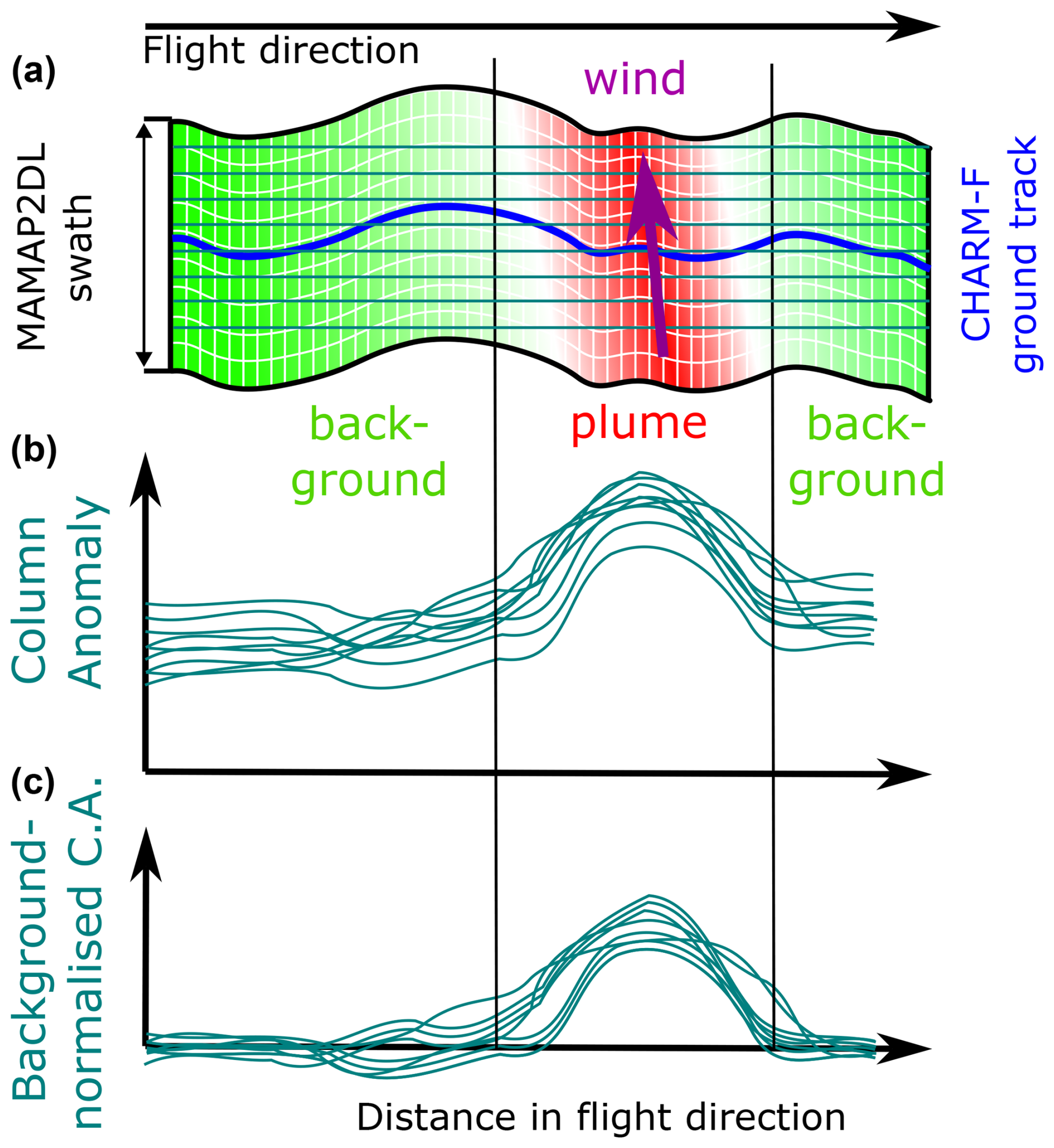
Figure 4 These schematic diagrams explain the principle used to estimate the CH₄ fluxes from the measured MAMAP2DL anomaly maps and CHARM-F anomalies. Panel (a) shows schematically the MAMAP2DL flight leg with the flight direction parallel to the x axis. The wind direction is approximately perpendicular to the flight direction. Horizontal dark-cyan lines indicate the added cross-sections for which the fluxes are computed. Vertical black lines, parallel to the y axis, separate the plume and background areas. The latter is used to normalize the entire cross-section and to compute the CH₄ anomalies within the plume area. The (10 m wide) CHARM-F ground track is depicted in blue. Panel (b) shows the column anomalies along the cross-sectional lines from panel (a). Panel (c) shows the normalized cross-sectional lines from panel (b) normalized by the background observation of the respective cross-section.

Next, we apply n cross-sections parallel to the x axis (dark-cyan solid lines in Fig. 4a) evenly distributed across the swath, and we define plume and background areas as indicated in Fig. 4 based on visual inspection of the plume signal across the entire swath, similar to the approach taken in other publications (e.g. Krings et al., 2018; Krautwurst et al., 2017; Frankenberg et al., 2016). To compute the CH₄ anomalies along one cross-section, we normalize it by the observations in the local background area (i.e. the cross-section is divided by values from a straight line which has been fitted to observations in the background only). This approach also accounts for smooth atmospheric concentration gradients or other systematic effects not considered during the retrieval.

The process of estimating the CH₄ background-normalized column anomalies is shown schematically in Fig. 4a to c. The objective of this sampling approach is to determine representative fluxes of one leg by considering as much available information as possible. Therefore, the number n of cross-sections is chosen such that the swath is well covered (i.e. every 10 m) and the number has basically no effect on the average flux of one leg calculated later. In the same manner, one cross-section is sampled with a sufficient number of points (i.e. every 10 m) so that changing this sampling also has effectively no effect on the flux anymore. As a result, Eq. (1) simplifies to become

$$\begin{array}{}\text{(2)}& F_{\mathrm{M}\mathrm{2}\mathrm{D},\mathrm{cs}}=f\cdot \mathrm{\Delta }x\cdot u\cdot \cos \left(\mathit{\alpha }\right)\cdot \sum _i\mathrm{\Delta }{V}_i,\end{array}$$

as wind speed u, angle α, and length element Δx are constant for one cross-section. The wind speed and direction are calculated at the position and overflight time of every leg from European Centre for Medium-Range Weather Forecasts (ECMWF) ERA5 fields (see Sect. 2.1.4 or Appendix D for validity of ERA5 data during the flight). We assume effective mixing of the emissions in the boundary layer and thus average the wind over all layers in ERA5 from the bottom to the top of the BL. Each layer is weighted by its number of air molecules. For an individual leg, the same winds are applied to the MAMAP2DL and later also to the CHARM-F observations for the flux calculation. The average flux F_M2D, leg for an entire MAMAP2D leg is computed by

$$\begin{array}{}\text{(3)}& F_{\mathrm{M}\mathrm{2}\mathrm{D},\mathrm{leg}}={\displaystyle \frac{{\sum }_{i=\mathrm{1}}^n{F}_{\mathrm{M}\mathrm{2}\mathrm{D},{\mathrm{cs}}_i}}{n}},\end{array}$$

where n is the number of cross-sections of one leg. The errors of the fluxes for one cross-section F_M2D, cs and of the average flux of one leg F_M2D, leg are then computed by error propagation using the errors on the individual parameters used in Eq. (2), as explained in Appendix F.

However, the above approach does not allow a one-to-one comparison of fluxes between those determined from the measurements made by the imaging MAMAP2DL and those made by the 1D CHARM-F instruments. Both datasets are actually distorted by the aircraft movement (i.e. predominantly the aircraft roll). The straight cross-sections introduced above for MAMAP2DL do not follow the distorted CHARM-F ground track. However, as seen in Fig. 4a, the CHARM-F ground track follows one fixed MAMAP2DL viewing angle approximately in the middle of the swath because the effect of the distortion is the same for both instruments. Therefore, Eq. (1) is directly applied to the measurements, with each parameter being evaluated individually for one measurement; i.e. the wind speed, direction, and length segment are not constant anymore. The resulting CHARM-F flux is then representative for this one leg. The definitions of plume and background areas remain the same.

Independent of the applied approach for MAMAP2DL or CHARM-F data described above, the fluxes from several legs, computed by Eq. (3), are then averaged again to derive the mean emission rates F_{M2D, ar-aver} and F_{CHARM-F, ar-aver}⁷ of certain areas in the measurement area for the respective instrument

$$\begin{array}{}\text{(4)}& F_{\text{M2D or CHARM-F, ar-aver}}={\displaystyle \frac{{\sum }_{i=\mathrm{1}}^p{F}_{{\text{M2D or CHARM-F, leg}}_i}}{p}},\end{array}$$

where p is the number of legs. This applies, for example, to the area in the lee of the two waste treatment areas, which is representative of the total emissions from the measurement area.

3 Results

3.1 Observed column enhancements over Madrid and source attribution

Figure 5 visualizes the retrieved and orthorectified CH₄ column anomaly maps derived from the MAMAP2DL measurements (Fig. 5a, as described in Sect. 2.2.1) and the XCH₄, given as 3 s averages, derived from CHARM-F data (Fig. 5d, as described in Sect. 2.2.2), for the different remote sensing legs acquired at a flight altitude of ∼ 7.7 $\mathrm{km}\mathrm{a}.\mathrm{g}.\mathrm{l}$. Both datasets clearly show CH₄ enhancements (in red) located at or downwind of the waste treatment areas, whereas, upwind or southwest of the Pinto landfill in the bottom-left corner, there are no indications of inflow of external enhanced CH₄ in the measurement area. These observations are also confirmed by two legs flown in along the wind direction at two different flight altitudes (see Appendix A and Fig. A1 for details). Especially for the Pinto landfill, there is a clear plume visible in both overflights, ∼ 2.5 h apart from each other.

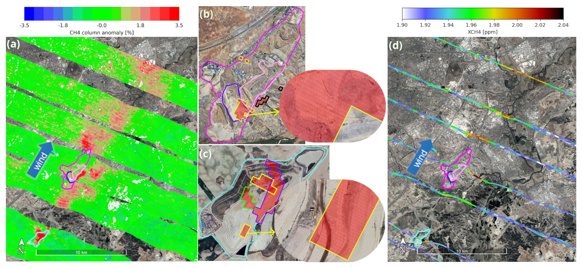
Figure 5 Retrieval results from the airborne remote sensing instruments. Panels (a) and (d) show the retrieved CH₄ column anomalies from MAMAP2DL and the XCH₄ from CHARM-F, respectively. Panels (b) and (c) are zoomed pictures of the two landfills including the MAMAP2DL ground scenes in red with the largest anomalies only (only those larger than ∼ 4 % for VTP or Las Dehesas in panel (b) and larger than ∼ 8 % for Pinto in panel (c); see main text for details). The different colours of the borders around those ground scenes in panels (b) and (c) mark the enhancements observed in different flight legs; e.g. yellow represents the leg flown in along the wind direction shown in Fig. A1a. The small insets in panels (b) and (c) zoom in further, detailing some activities across the areas with the largest observed enhancements. The Google imagery shown was recorded in August 2022. The waste treatment areas are encircled by different solid coloured lines: cyan for the Pinto landfill, magenta for the VTP, pink for the Valdemingómez landfill, and purple for the Las Dehesas landfill. The map underneath is provided by © Google Earth, using imagery by Landsat/Copernicus, Maxar Technologies.

The highest CH₄ concentrations are observed at or close to landfills. CH₄ hotspots, with peak enhancements of around 17 %, are located at the eastern part of the Pinto landfill according to the MAMAP2DL imaging data. This hotspot is also captured by the CHARM-F instrument with XCH₄ of up to 2.28 ppm.

The insets Fig. 5b and c show more details of the individual landfills, including the locations of the highest column anomalies, which were identified in different overflights. Marked regions in the southeast of the landfills are areas which are most probably responsible for a large fraction of the observed emissions. They were selected by analysing the flight legs (those flown perpendicular to the wind direction and those flown in the wind direction) over the landfills to find the ground scenes with the highest column enhancements (only ground scenes above a certain threshold are shown; see Fig. 5 for more details). The assumption is that the CH₄ is most concentrated just above or very close to a source, as it is not yet dispersed (horizontally), leading to the highest observed column enhancements. However, there is a residual uncertainty associated with this method, as, by chance, high column enhancements could also be observed further away due to turbulent transport. Columns are also modulated by the prevailing wind speed at the time of release into the atmosphere and by local atmospheric turbulence. Both can change during a measurement flight. However, if the highest column anomalies during multiple overflights point to the same region, there is a high probability that this region is acting as a source.

The Google Earth imagery recorded in August 2022 (the same month and year as our flight) clearly shows that these hotspots are directly located over active landfill areas where waste is deposited. The CH₄ plumes clearly begin over these areas of the Pinto and Las Dehesas landfills (see Figs. 5 and A1 and discussion on the step-wise increase in the fluxes in Sect. 3.3). However, we cannot exclude that other parts, closed cells of the landfills or facilities located in these waste treatment areas, also contribute (weakly) to the observed CH₄ plume but are partly masked by CH₄ released further upwind. For example, in the northwestern part of the VTP, there are also hotspots identified (two ground scenes outlined in yellow in Fig. 5b) from the along-wind leg (Fig. A1a), which could be advected there or released from the waste treatment plants (La Paloma and Las Dehesas) immediately to the south. However, as a second overflight (Fig. A1b) shows no enhancements, it is probably the former.

3.2 Column comparison between MAMAP2DL and CHARM-F

Figure 5 shows a good visual agreement between the column anomalies of the passive MAMAP2DL and the XCH₄ of the active CHARM-F instruments. In order to perform a more rigorous comparison between the two types of atmospheric CH₄ columns, we convert the XCH₄ partial columns derived from CHARM-F to total-column anomalies (see Sect. 2.3). We then identify the ground scene in the MAMAP2DL swath which corresponds to the CHARM-F measurements, which are approximately located in the middle of the MAMAP2DL swath. This procedure ensures the selection of observations, where both instruments see similar ground scenes and air masses.

Figure 6 shows a typical example comparison for one leg. The two different types of observations have been processed as explained previously; i.e. the plume anomalies have been processed as described in Sect. 2.3, and the CH₄ fluxes have been estimated as described in Sect. 2.4. The background-normalized column anomalies shown agree well within their respective errors inside and outside of the plume. Even more pronounced structures in the CH₄ concentration, as encountered on the right-hand side (∼ 6 to 15 km distance), are identified by both instruments. The fluxes from the two cross-sections shown deviate by only 0.1 t h⁻¹ or 1 %.

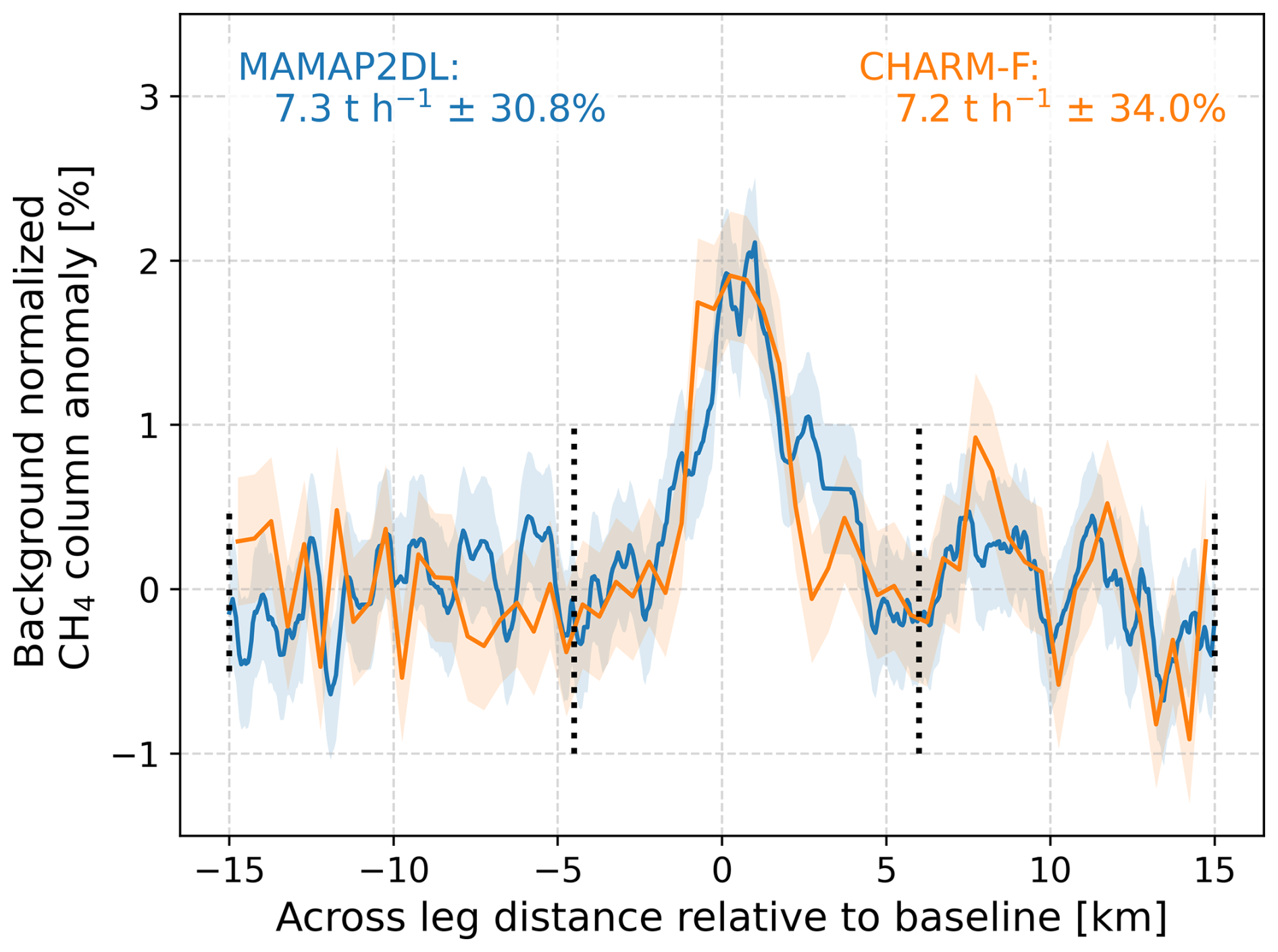
Figure 6 The background-normalized CH₄ column anomalies for CHARM-F (orange) and the co-located MAMAP2DL (blue) observations for one flight leg collected between 11:42 and 11:46 UTC are shown. Vertical dotted lines separate the plume and background areas. Shaded areas represent the random error (single-measurement precision) of the retrieved column anomalies of the respective instruments. The computed fluxes for the cross-sections according to Eq. (1) and the corresponding errors (MAMAP2DL: Eq. F1; CHARM-F: Eq. F10) are given by the text insets. For graphical presentation only, the MAMAP2DL data are smoothed by a 500 m kernel to match the spatial resolution of CHARM-F in the along-flight direction. The flux, error, and uncertainty range are, however, based on the ∼ 110 × 110 m² data.

More generally, when comparing fluxes estimated using measurements of MAMAP2DL with those derived from CHARM-F observations from all flight legs (see Fig. E1), the averaged absolute difference between them is ∼ 1.2 t h⁻¹ or ∼ 13 % excluding the flight legs upwind and directly over the Pinto landfill (see Sect. 3.3 for reasoning). These differences may be due to (a) different but overlapping opening angles of the two instruments and the resultant spatial resolution of the ground scene widths of 110 m and 10 m, respectively; (b) different paths through the atmosphere of the electromagnetic radiation used to measure methane absorption; or (c) differences in the algorithms used to retrieve the columns, e.g. how they deal with variable surface reflectivity. Consequently, observed air masses are different.

Typically, the errors of the fluxes are around or below 30 % of the respective flux and are similar for MAMAP2DL and CHARM-F.

3.3 Derived landfill emission rates

Using imaging MAMAP2DL observations, we also computed the fluxes within the different legs (see Sect. 2.4). The results are summarized in Fig. 7, which also includes the cross-sectional fluxes derived from the CHARM-F instrument already computed and introduced in Sect. 3.2.

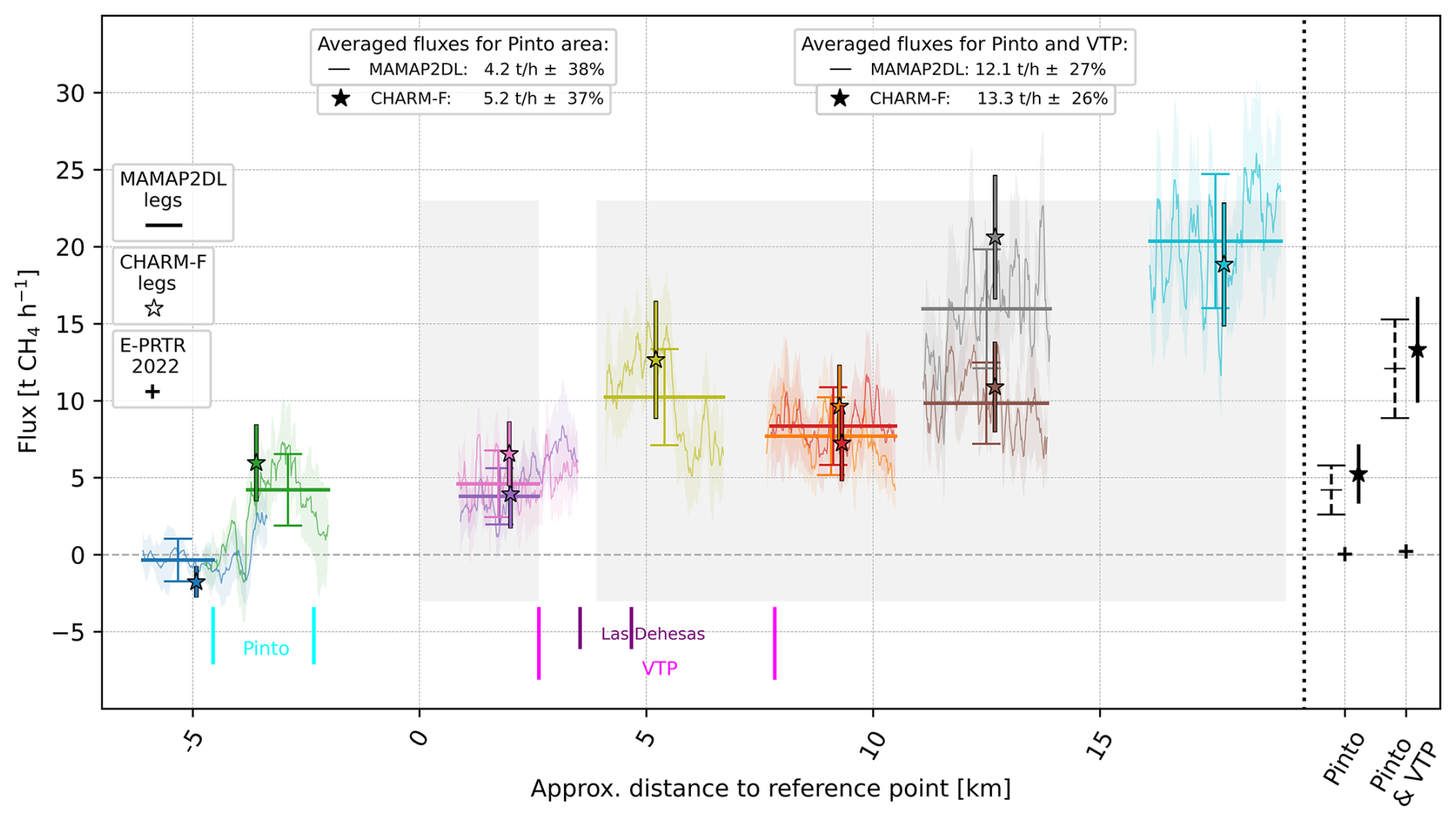
Figure 7 This plot shows the evolution of the CH₄ flux values upwind of the waste treatment areas (−5 km) to downwind (> 8 km). Cyan, purple, and magenta vertical lines identify the locations of the two investigated waste treatment areas. The coloured thin solid lines are the values of the cross-sectional fluxes across the different MAMAP2DL legs and exhibit a high variability most likely due to atmospheric variability and turbulence on that day. Corresponding shaded coloured areas show the errors (estimated using Eq. F1). The averaged flux and error (Eq. F3) of one leg are given by the coloured bold horizontal lines and the error bars, respectively. The averaged fluxes or emission rates and their errors (Eq. F6) estimated using MAMAP2DL observations for the two areas (in between Pinto and the Valdemingómez technology park (VTP) and in the lee of the VTP) are the dashed black lines in the right panel of the figure. Coloured stars and vertical bars give the fluxes and errors (Eq. F10), respectively, estimated using the CHARM-F measurements. Black stars and bars in the right panel are the averaged fluxes or emission rates and their errors (Eq. F11) over the same areas as for the MAMAP2DL observations. The two areas over which emission rates are computed are indicated by the grey shading. The pluses in the right panel additionally indicate the reported emissions for the Pinto area, and for both the Pinto area and the VTP, for the year 2022 assuming constant emission during the year.

Based on the MAMAP2DL observations, the fluxes exhibit a step-wise increase at the location of landfills as expected, from left (upwind) to right (downwind). The upwind leg at −5 km shows no significant inflow of enhanced CH₄ and a steep increase directly over the Pinto landfill. Between the Pinto and the VTP, the flux or emission rate stabilizes at 4.2 t h⁻¹ (±38 %) before increasing to around 12.1 t h⁻¹ (±27 %) on average at and after the Las Dehesas landfill. However, the cross-sectional fluxes show some variability from flight leg to flight leg (see the bold horizontal coloured lines, representing averaged values over one MAMAP2DL leg) and variability within one leg (see the thin solid coloured lines). Furthermore, the retrieved column anomalies in Fig. 5 and the cross-sectional fluxes in Fig. 7 show no sign of accumulation of CH₄ as, for example, in the valley between the two landfills (see Sect. 2.1.1 for a brief discussion of the local topography). Adding the fluxes derived from the CHARM-F observations to the figure (coloured stars) reveals very good agreement between active and passive remote sensing (thin solid coloured lines) data as already indicated in Sect. 3.2. Computing average fluxes or emission rates from the CHARM-F observations alone yields 5.2 t h⁻¹ (±37 %) for the Pinto landfill and 13.3 t h⁻¹ (±26 %) for both waste treatment areas combined.

The first two flight legs were deliberately designed so that, in the blue leg, CHARM-F sampled background conditions upwind of the Pinto landfill, while MAMAP2DL already partially covered the source area. Conversely, during the green leg, CHARM-F measured directly over the Pinto landfill, whereas the MAMAP2DL swath still included parts of the upwind background. For the averaged flux between the two landfills, the flight leg directly over the Pinto landfill (i.e. the green lines and star in Fig. 7) has been omitted. There, the plume might be still restricted to the surface and the wind speed is highly biased due to the strong vertical wind gradient (see Fig. D2a). Over the Las Dehesas landfill, although there are new emissions emerging at the bottom, the plume from Pinto is assumed to already be well mixed. Therefore, this leg is included in the flux average.

3.4 Discussion on uncertainties

The estimation of errors or uncertainties is extensively discussed in Appendix F, and Table 1 lists the uncertainties for the different components we assumed in our error analysis. Table 2 summarizes the effect of the these components on the computed fluxes.

Table 1 Summary of relevant error sources used during the error analysis described in Appendix F. See Table F1 for further explanation of error sources.

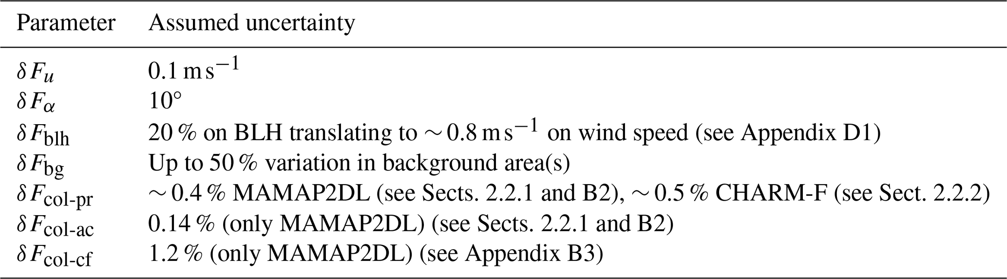
Table 2 Summary of computed error components for the averaged flux downwind of the two waste treatment areas according to Appendix F. Values are given as percentages of the respective downwind fluxes: 12.1 t h⁻¹ for MAMAP2DL and 13.1 t h⁻¹ for CHARM-F. “X” stands for MAMAP2DL or CHARM-F according to nomenclature in Appendix F2 and F3, respectively.

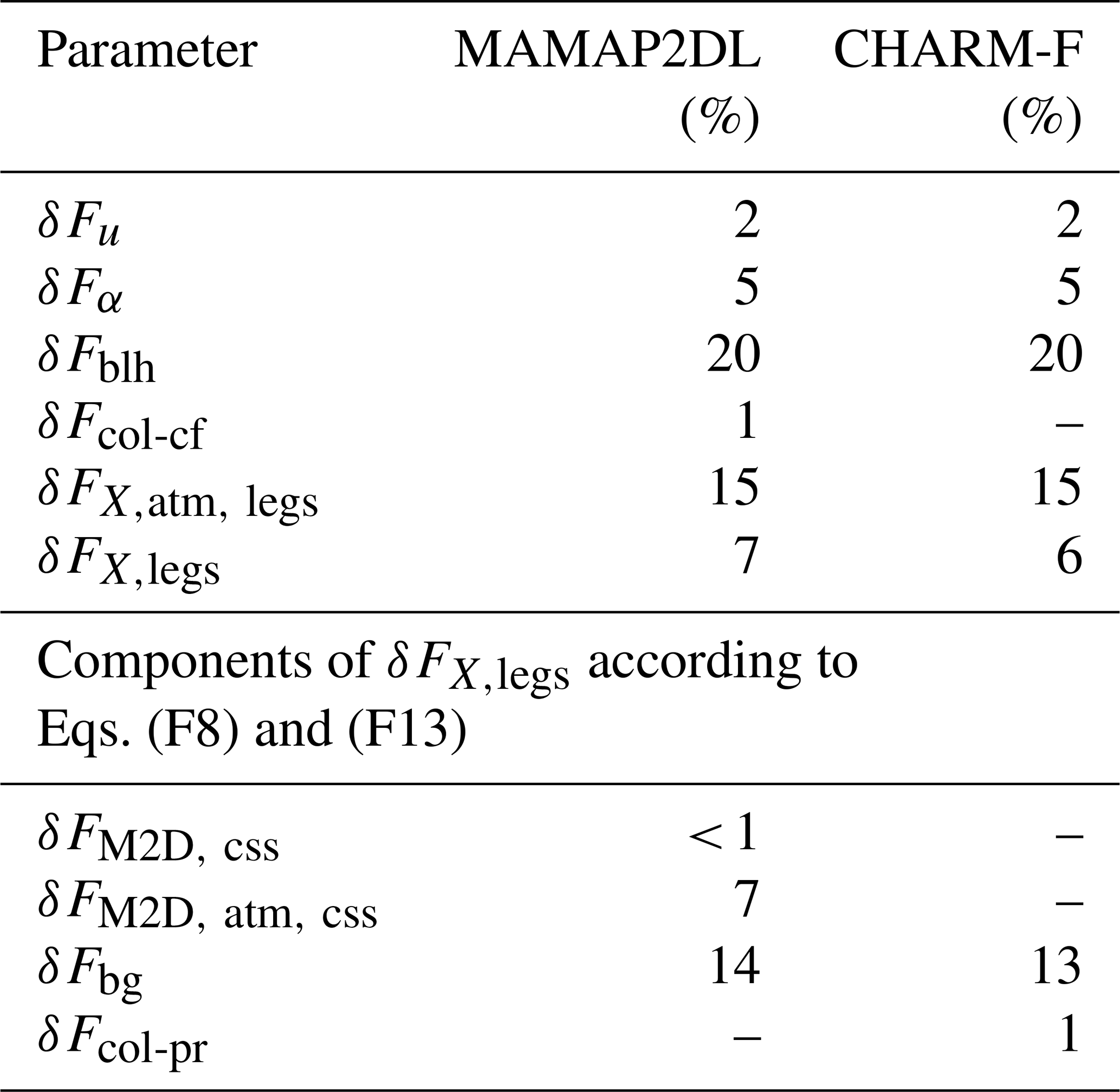
3.4.1 Individual error components

The uncertainties of our estimated fluxes are on the order of 25 to 40 % of the respective flux for the different spatial scales (single cross-sections/legs or areal averages) and are therefore quite similar for the different spatial scales. This is due to the fact that the major error source, BLH (δF_blh: ∼ 20 % error on the flux; see Table 2), consequently affecting the averaged wind speed over the BL, is systematic and therefore cannot be reduced by averaging over several cross-sections or legs. The error on the wind speed (δF_u: ∼ 2 %) and wind direction (δF_α : ∼ 5 %) itself, although also a systematic one, has only a limited influence. The other two important error sources are plume distortions caused by atmospheric turbulence ($\mathit{\delta }{F}_{X,\mathrm{atm},\mathrm{legs}}$: ∼ 15 %) and the limits for the background area (δF_bg: ∼ 14 %). The latter is especially pronounced on the scales of legs, as it reduces by averaging over several legs. The column single-measurement precision (δF_col-pr: < 1 %) of the two instruments, or the remaining systematic offset (δF_col-ac: < 2 %), and the conversion factor error (δF_col-cf: < 2 %) of MAMAP2DL lead to negligible errors on the computed fluxes due to the relatively large spatial extent and large enhancements of the observed plume signals.

The major error source is the uncertainty in BLH, which has a significant influence on the averaged wind speed applied in the flux computation. As stated above (Sect. 2.1.4 and Appendix D), we used atmospheric measurements of wind speed, direction, and potential temperature collected during one ascent and one descent to validate and correct the ERA5 model estimates. Based on the two measured profiles and the overestimation of the BLH in ERA5 compared to these profiles, we apply a correction reducing the ERA5 BLH by ∼ 17 % on average. We assume that this correction is also applicable to ERA5 data up to 2 h earlier when the remote sensing measurements started. Due to the strong vertical gradient in wind speed, this also reduces the averaged wind speed by ∼ 24 % and leads to the same relative reduction in the fluxes. The uncertainty of the BLH estimates itself is 20 %, which consequently translates into a wind speed error of 0.8 m s⁻¹ on average.

Additionally, to estimate the accuracy of the ERA5 wind data, we compare them to the BAHAMAS measurements. The averaged deviations are only 0.05 m s⁻¹ and 0.8°. Therefore, we assume that the error on the modelled wind speed within the BL is 0.1 m s⁻¹. For the wind direction, we compared the modelled one with the visually observed plumes in Google Earth imagery and concluded an uncertainty of ∼ 10°.

Other important error sources are the limits for the background area and plume distortions caused by atmospheric turbulence. Depending on the spatial scale, they are reduced by averaging the estimated CH₄ fluxes from multiple cross-sections. For example, the effect of the atmospheric variability reduces if more independent legs or cross-sections are collected (either spatially or temporally separated). This variability is quantified by the standard deviation (SD) over all legs of one area where a constant flux is expected or over the individual cross-sectional fluxes within one leg. We assume that the fluxes are independent for different legs, as they are recorded at different times and/or locations but have a correlation length of around ∼ 400 m within one MAMAP2DL leg, resulting in seven independent fluxes across one leg.

Even if correlation between all fluxes of one leg is assumed, the relative error on the averaged downwind flux would only increase from 27 % to 28 %. The effect would be slightly larger for the averaged flux between the two landfills (38 % vs. 45 %) and for single legs (7 % vs. 18 %). The errors are still dominated by the systematic wind errors. As we use the standard deviation to quantify the variability, it might also be partly influenced by measurement error and the error introduced by the background normalization.

For MAMAP2DL, the uncertainty from the conversion factor related to the magnitude and change in the BLH during the flight time is also a systematic error source and scales with the retrieved anomalies. This is not reduced by multiple cross-sections or legs and has the same influence on the cross-sectional fluxes within one MAMAP2DL leg and on the averaged total flux from the two waste treatment areas.

3.4.2 Potential additional sources

The most downwind leg in Fig. 7 (cyan leg) shows a high variability in the computed fluxes from the MAMAP2DL observations across the first two-thirds of the leg, whereas the last third, which is also located downwind of the position of the CHARM-F observation, shows a consistently more stable and higher flux. This might be related to potential additional CH₄ emissions from an industrial area located there (40.433° N, 3.491° W), which also includes a “Planta de Combustible” (fuel plant, not listed in E-PRTR), several storage tanks, and a wastewater treatment plant. Excluding this latter part of the MAMAP2DL leg would reduce the mean flux of this MAMAP2DL leg from 20.4 to 19.1 t h⁻¹ but reduce the average over the entire area by only 0.1 t h⁻¹.

Furthermore, there is also the possibility that other CH₄ sources located in the measurement area could affect the observed emission rates. Depending on whether these sources are in the plume area or the background area, they either contribute to the emissions or reduce them. If they were evenly distributed around the area, the effect on the estimated emission rate would be negligible. We estimated this effect by analysing the CH₄ emissions reported in the Emissions Database for Global Atmospheric Research (EDGAR) v8.0 (Crippa et al., 2023). We aggregated all CH₄ emissions in our measurement area except for the source categories 4A and 4B (solid waste disposal and biological treatment of solid waste), which are our targets. Consequently, in the worst case, the resulting impact on our estimated emission rates could be up to approximately 2 t h⁻¹ at maximum or around 15 % of our total emission rate estimated according to EDGAR v8.0. Additionally, no other sources stand out in our column observations.

3.4.3 Potential plume accumulation effects

As discussed in Appendix D1 and shown in Fig. D2b, before the start of the remote sensing part of the flight at 11:00 UTC, the wind direction changed from around 130 to 210°. Additionally, during the entire flight time, there was a very strong vertical wind gradient with ∼ 1 m s⁻¹ at the ground and up to ∼ 10 m s⁻¹ at the top of the BL (Fig. D2a). In particular, the turn in wind direction directly before our measurement started could potentially have created an area with enhanced CH₄ concentrations due to accumulation (a “CH₄ puff”), which would subsequently have been advected in wind direction. Surveying such a puff would also lead to increased fluxes.

The grey and cyan leg in Fig. 7 would indicate these enhanced fluxes compared to the remaining legs. Assuming that, during the time of the remote sensing measurement, a mean wind speed of ∼ 3.9 m s⁻¹ prevailed, and that these legs were acquired around 90 min after the start at 11:00 UTC, would lead to a travel distance of 21 km of the observed air masses. A distance of 21 km would roughly correspond to the southern part of the Pinto waste treatment area. Excluding the two legs from the downwind average would lead to a mean flux of 9.6 t h⁻¹ instead of 12.7 t h⁻¹. Additionally, the change in wind direction also caused some residual plume structures over the city of Madrid. A potential influence of this residual plume on our background determination is covered by the respective error δF_bg.

To investigate these effects further and to verify our assumption of CH₄ accumulation would, however, require more sophisticated model simulations and is not possible with a simple and fast mass balance approach. Applying model-inversion-based flux estimation methods is beyond the scope of this publication but will be addressed in a follow-up paper that is currently in preparation.

4 Comparison of emission rates determined in this study with other estimates

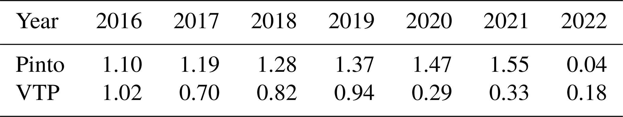
The waste treatment areas Pinto and VTP have reported emission rates of 0.35 kt yr⁻¹ (or 0.04 t h⁻¹ assuming constant emissions throughout the year) and 1.58 kt yr⁻¹ (or 0.17 t h⁻¹), respectively, in E-PRTR for the year 2022. Our observations were collected within 2 h on 4 August 2022. This represents a snapshot of estimated emission rates, and they should not be lightly extrapolated to annual averages. Landfill emissions usually exhibit some temporal variability and are modulated, for example, by emissions caused by leakages; activities across the landfill when waste is deposited; atmospheric parameters such as pressure changes, temperature, and wind speed; or temperature and humidity conditions within the landfill (e.g. Cusworth et al., 2024; Kissas et al., 2022; Delkash et al., 2016; Xu et al., 2014; Trapani et al., 2013; Poulsen and Moldrup, 2006).

However, over the past years, other studies using observations of a limited period derived similar emission rate estimates as observed by us. The most recent is the webstory from ESA (2021) using satellite data from TROPOMI and GHGSat in August and October 2021. They reported total emission rates of 8.8 t h⁻¹ with one of the sources emitting 5.0 t h⁻¹, without mentioning landfill names. However, in the GHGSat images on the website, the Pinto and Las Dehesas landfills are identified as part of their target area. Although these estimates are from the preceding year, partly from the same season, they agree well with our results. Additionally, based on the available imagery, one main plume appears to originate, at least partly, from the already closed and covered area of the Las Dehesas landfill. Although we cannot exclude outgassing from closed parts of this landfill, our CH₄ hotspots are predominantly located over the active areas of the landfills.

In 2018, another study used ground-based and satellite observations to also estimate emissions of Madrid's landfills (Tu et al., 2022). Their ground-based observations were collected between the end of September and the beginning of October 2018, and their resulting flux is ∼ 3.5 t h⁻¹. This flux was assigned to the Valdemingómez waste plant. Satellite data were analysed over the period May 2018 to December 2020. Estimated emission rates are 7.1 t h⁻¹ (±0.6 t h⁻¹) for the entire area.

A ground-based investigation in that area was undertaken from 1 to 3 March in 2016. Sánchez et al. (2019) used specifically designed flux chambers to measure CH₄ emission from the already full and closed parts (or cells) of the Las Dehesas landfill north of the still-active area. They estimated 1.1 t h⁻¹ on average for this part, which accounts for approximately half of the total designated landfill area of ∼ 0.6 km². The values for the 95 % confidence interval are given with 0.4 to 2.8 t h⁻¹. However, their averaged value would correspond to around 9 % of our total emission rate derived for the entire area also including the Pinto landfill.

Over the past years, all these estimates indicate consistently high emission rates of up to 7 to 9 t h⁻¹ for both waste treatment areas, although they are made over short periods (with the exception of the estimates using satellite observations⁸). Our estimated emission rates for the two areas are at the upper end of this range (12.7 or 9.3 t h⁻¹ if the CH₄ puff hypothesis is applicable) and also indicate disagreement with the reported values in E-PRTR (see Table 3). Interestingly, the reported emissions of the Pinto landfill site decreased by a factor of almost 40 from 2021 to 2022, which could potentially be related to the change in reporting methodology (see Sect. 2.1.1).

Table 3 Reported CH₄ emission rates in E-PRTR for the Pinto area and the VTP in t h⁻¹ assuming constant emissions throughout the year.

The locations of high human activity and waste deposition correlate with the highest observed column concentrations. We infer that these locations on the landfill are the main origin of our observed emissions. These active areas were also identified by Cusworth et al. (2024) as CH₄ emission sources. However, it is unclear whether these emission hotspots exist only during the day, when work is done on the landfill, or also at night. The degree of correlation between emissions and activity is unclear, and these emissions should actually cease when a cell is completed and closed. Local process-based bottom-up modelling of emissions of waste deposition is challenging due to the unpredictability of exact locations and practices. This may explain some of the discrepancies between the inventory and the top-down estimates (Balasus et al., 2024).

5 Summary and conclusion

The reduction in anthropogenic CH₄ emissions has been proposed as a target for climate mitigation strategies, due to CH₄'s relatively short tropospheric lifetime. In spite of this objective, knowledge of the CH₄ emissions from many anthropogenic sources and, in particular, landfills, even though these emissions account for a significant fraction of the global anthropogenic CH₄ budget, are still uncertain. Relevant examples are the recent discussions of the emissions from landfill sites in Madrid, the capital of Spain. Exceptionally high CH₄ emission rates have been reported using both ground-based and satellite-borne observations in the year 2021 and before.

To examine these CH₄ sources and to estimate their emissions, we undertook a measurement flight on 4 August 2022 as part of the CoMet 2.0 mission. In this study, for the first time, the passive imaging MAMAP2DL and active lidar CHARM-F remote sensing instruments flew aboard the same platform, the German research aircraft HALO, and successfully co-located and independent measurements were made. During the first part of the flight, remote sensing column observations were acquired. MAMAP2DL collected 28 ground scenes with a spatial resolution of ∼ 110 × 110 m² within an ∼ 3 km swath for a flight altitude of 7.7 $\mathrm{km}\mathrm{a}.\mathrm{g}.\mathrm{l}$. CHARM-F recorded ground tracks with a spatial resolution of ∼ 500 m in the flight direction, due to averaging, and ∼ 10 m across.

In total, 10 flight legs, aligned perpendicular to the prevailing wind direction, were flown at several distances up- and downwind of the two waste treatment areas Pinto and VTP, including the Las Dehesas landfill. Exploiting the design of the flight plan, emissions from the two landfill sites were separated and estimated by combining the retrieved CH₄ column anomalies with model wind data from ECMWF ERA5. Additionally, from the overflights above the landfill areas in combination with CH₄ imaging data, potential source locations on the landfills were identified.

The BL was physically characterized by the measurements of vertical atmospheric profiles of meteorological parameters and trace gases within the BL. This supported our analysis of the remote sensing data and was used to validate the ERA5 model data for that day. As the remote sensing data were acquired well above the BL, we relied on models for (wind) data within the BL.

The emissions from the two landfill sites were sufficiently separated for our methods by the two remote sensing instruments with an observed emission rate of ∼ 5 t h⁻¹ for the Pinto area, while the combined emission rate of Pinto and VTP was ∼ 13 t h⁻¹. The errors on these CH₄ emission rate estimates are around 26 % to 38 % of the given fluxes (or 1.9 to 3.5 t h⁻¹) and are dominated by the knowledge of the BLH in combination with a strong vertical wind gradient and the separation between plume and background areas. Moreover, the measured fluxes and emission rates are influenced by atmospheric turbulence. This results in the flux variation in different legs expressed as standard deviation over all legs in the downwind area of up to ∼ 5 t h⁻¹. We conclude that a sufficient number of independent flight legs are required to minimize the error from turbulent flow in the estimation of the fluxes from observed plumes.

This was the first time that emissions were observed and quantified simultaneously by two different and independent active and passive remote sensing techniques. The comparison of fluxes retrieved using the measurements of the active and passive remote sensing instruments shows that the two estimates are in very good agreement. To ensure comparability of the flux estimation using the different remote sensing approaches, we also used identical wind speeds for individual legs. Absolute differences are 13 % of the respective fluxes on average. These differences may be explained by the different ground scene sizes observed by the two instruments, which are 10 and 110 m for CHARM-F and MAMAP2DL in the across-flight direction. Consequently, they measure different but overlapping air masses in the plume. The agreement between the two different techniques also increases our confidence that the emission rates are as high as our estimates. The complementarity of the active and passive instruments also shows good prospects for their joint deployment on spaceborne platforms.

For source attribution, the imaging data of the MAMAP2DL instrument were utilized. The determination of the exact source location is limited by a combination of the ground scene size of ∼ 110 × 110 m², the accuracy of the orthorectification process itself being estimated to be better than 110 m, and modulation by local winds. The highest column enhancements and the “start” of plumes, indicating the origin of the emissions, were observed over active parts of the landfills, where the garbage is deposited, towards the southeast for Las Dehesas and in the eastern part of Pinto. In the same regions, CHARM-F observes the largest column enhancements. This implies significant emissions from areas which are not yet managed during nominal operations but are probably also not sufficiently covered by the reporting. Nevertheless, the question remains about nighttime and weekend emissions, when there is less or no activity on the landfill.

A crucial parameter for the estimation of emission rates is the wind speed, which is particularly challenging to determine for remote sensing instruments, as they typically fly above the plumes and the BL. Here, we used modelled ERA5 data, which were validated by airborne measurements within the BL. On average, wind speed and direction disagree by only 0.05 m s⁻¹ and 0.8°, respectively.

However, larger deviations occurred for the BLH in ERA5, which was consistently lower in the comparison of ERA5 to the two measured profiles. Correcting for this discrepancy led to a decrease in the average wind speed used for the cross-sectional fluxes of ∼ 24 % due to the strong vertical wind gradient (present in both ERA5 model data and BAHAMAS wind measurements). This reduction in wind speed directly changes the estimated emission rates proportionately.

Our analysis shows the importance of knowledge and understanding of the characteristics of the BL during a measurement. While we had the privilege to compare in situ wind measurements with model data, even though at a later time of the day, emission estimates based on satellite data rely on atmospheric parameters from models. Moreover, there is usually no possibility to validate the conditions during measurement times. Systematic errors, such as the BLH in combination with the strong vertical wind speed gradient, influence the estimated emission rates. They need to be identified and taken into account to minimize their impact.

Our calculated emission rates are in good agreement with previous top-down estimates, even though, strictly speaking, they are only valid for the time of the overflight. The prevailing winds in combination with the vertical distribution of the CH₄ emissions in the BL could introduce a common error in our emission rate estimate but not to an extent that we approach reported values assuming constant emission throughout the year, at least on 4 August 2022 during our flight. The fact that our emission estimates are a factor of 40 to 50 higher than reported values (assuming constant emissions) supports the inference that a major part of the emissions is unreported, especially as the reported emissions in E-PRTR fell by a factor of 10 from 2021 to 2022.

The methods used in this work are also applicable to planned satellite missions, such as CO2M and MERLIN. Nevertheless, the generally coarser resolution on the ground will lead to a reduced sensitivity for emission rates, particularly for somewhat dispersed sources. Also, the combination of active and passive remote sensing on a single satellite platform would show promise for the future, as the advantages of both methods can be synergistically exploited.

An additional analysis is currently being studied. This makes use of a transport model to constrain the influence of the (changing) wind field and the (vertical) mixing of the CH₄ plume during the measurement flight. We expect that the use of a transport model will resolve some of the issues encountered when the direction of the wind changes, i.e. residual plume structures over the city of Madrid and potential CH₄ accumulations. These are difficult to account for using the simple cross-sectional mass balance approach.

Appendix A: Further flight legs

Figure A1 supplements Fig. 5 with two additional flight legs, which were flown in along the wind direction. Therefore, they were not used for any flux estimates. However, they reveal further insights into possible source regions.

The flight leg in Fig. A1a was acquired at the same flight altitude as the legs shown in Fig. 5. The leg shown in Fig. A1b, on the other hand, was collected after the in situ part of the flight at around 13:34 UTC at a flight altitude of ∼ 1.6 $\mathrm{km}\mathrm{a}.\mathrm{g}.\mathrm{l}$. The reduced flight altitude also reduced the swath width of the MAMAP2DL imaging data from ∼ 3 km to 700 m and reduced the ground scene size from ∼ 110 × 110 to 24 × 24 m².

Interestingly, in the lower flight leg (Fig. A1b), CH₄ enhancements are observed at similar positions to those in the leg flown at higher altitudes (Fig. A1a) and in the perpendicular legs in Fig. 5a for the Pinto landfill in the south. However, no enhancements are visible across the VTP (Fig. A1b). This is in line with the legs flown perpendicular to the wind direction, in which the highest anomalies were observed in the southeastern part of the Las Dehesas landfill but not covered by the low flying leg. As the flight leg, acquired at lower flight altitude (Fig. A1b), was within the BL and therefore within the plume, caution needs to be taken with a quantitative interpretation of the MAMAP2DL column anomalies shown.

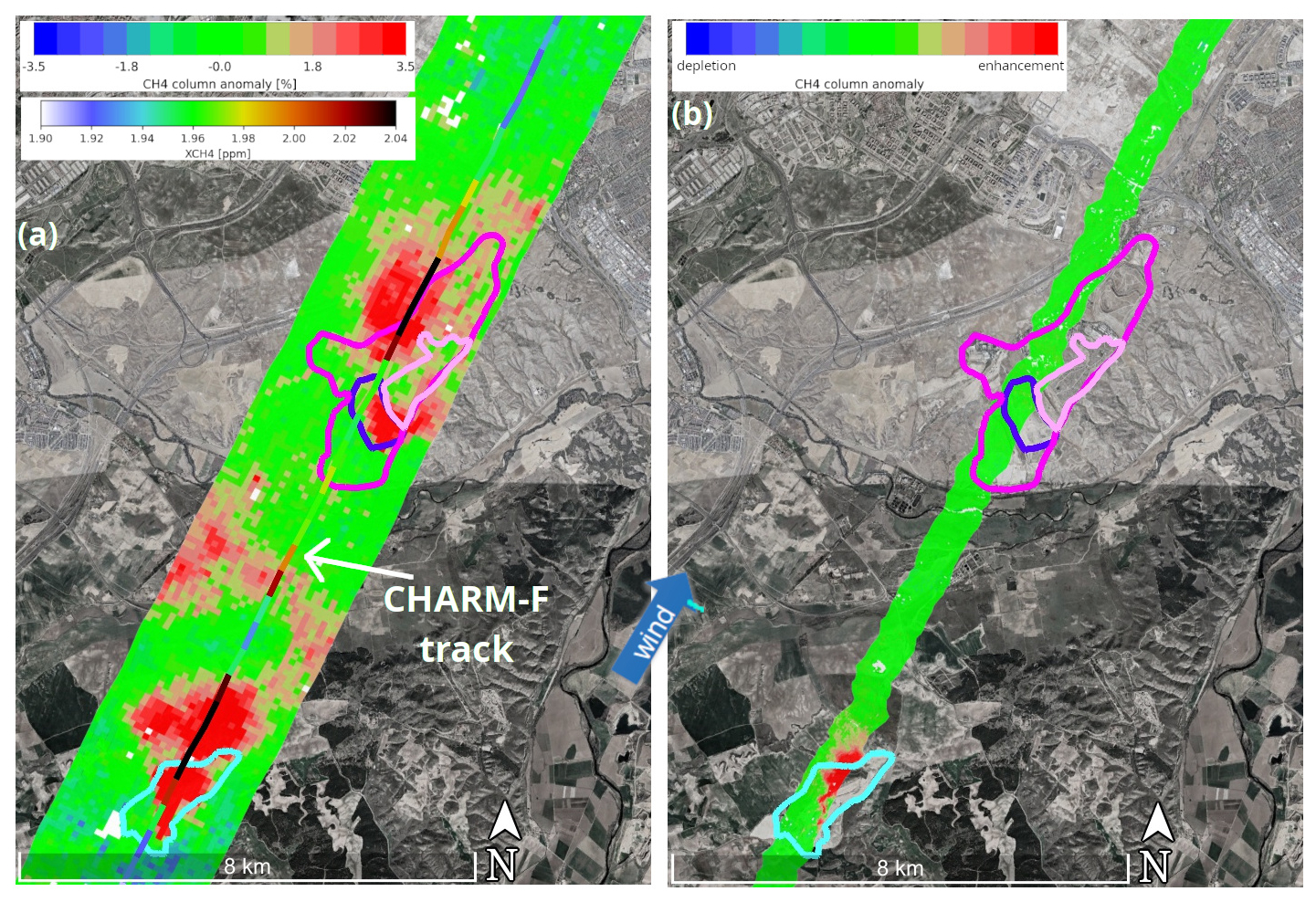
Figure A1 Similar to Fig. 5 but for the along-wind legs at flight altitudes of ∼ 7.7 $\mathrm{km}\mathrm{a}.\mathrm{g}.\mathrm{l}.$ (a) and ∼ 1.6 $\mathrm{km}\mathrm{a}.\mathrm{g}.\mathrm{l}.$ (b). In panel (a), the retrieved CH₄ column anomalies from MAMAP2DL data are overlaid by the XCH₄ from CHARM-F data. There are no CHARM-F data available for low flying altitudes due to saturation of the detectors. The map underneath is provided by © Google Earth, using imagery by Landsat/Copernicus, Maxar Technologies.

Appendix B: MAMAP2DL retrieval

B1 WFMD-DOAS

The WFM-DOAS retrieval has been extensively described in other publications (Krings et al., 2011; Krautwurst et al., 2021); thus, we focus here on the aspects which are important for the quality of the retrieved CH₄ column anomalies. The core of the retrieval is based on radiative transfer model (RTM) simulations (in our case with SCIATRAN v3.8; Mei et al., 2023; Rozanov et al., 2014) of radiances, which describe the general state of the atmosphere at the time of the measurement flight to our best knowledge. Differences between the modelled radiance and the measured radiance are described by fitting weighting functions⁹ to the model and minimizing the difference between the measurement and the modified model. An example for such differences is deeper absorption lines due to enhanced CH₄ from an emission plume in the atmosphere. The resulting fit factors are called profile scaling factors (PSFs) and are representative for the observed atmospheric CH₄ and CO₂ columns. The weighting functions, one for each fit parameter (in our case for CH₄, CO₂, H₂O, and temperature), describe the change in radiance due to a change in one of the listed parameters. Furthermore, we apply a 1D look-up table approach for the topography to account for strong variations in surface elevation during the retrieval process.

To represent the atmosphere by the modelled radiances as realistically as possible, vertical concentration profiles of the gases (CH₄, CO₂, H₂O), pressure, and temperature are needed. The model takes the properties of the reflecting surface into account. Multiple scattering by aerosols in the atmosphere is considered. Finally, geometrical factors, such as flight altitude, surface elevation, and solar zenith angle (SZA), are included in the calculations (see Table B1 for details on the parameters used). Figure B1 shows one example fit for the two fit windows which we use in this study. These are 1590.0 to 1635.0 nm for CO₂ and 1625.0 to 1672.5 nm for CH₄.

Table B1 Boundary conditions for the radiative transfer model (RTM) simulations for the remote sensing (RS) part at ∼ 7.7 $\mathrm{km}\mathrm{a}.\mathrm{g}.\mathrm{l}.$ of the flight over Madrid.

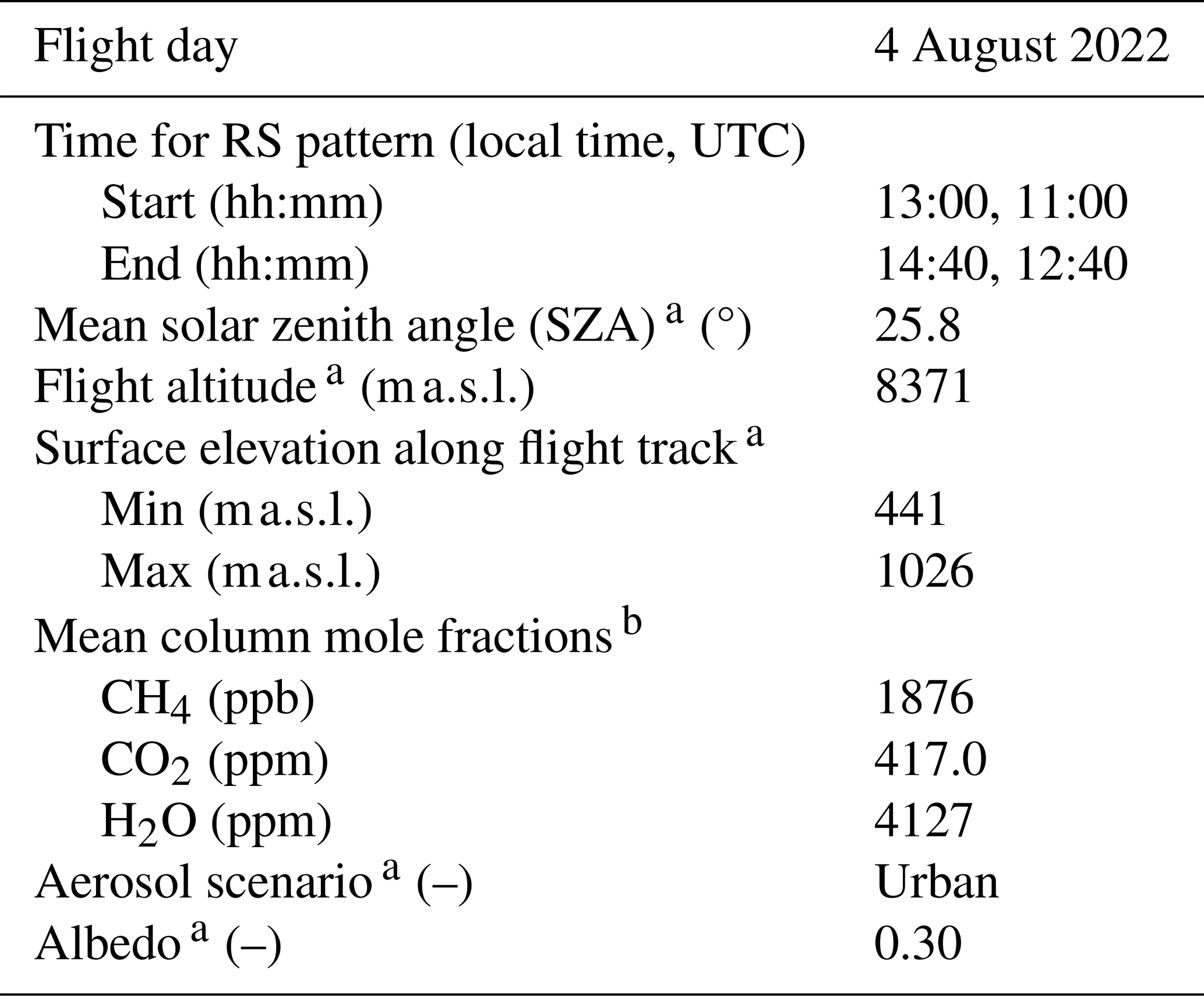
^a Estimated similarly to Krautwurst et al. (2021). ^b The vertical atmospheric profiles are taken from the US standard atmosphere (USCESA, 1976), which are adapted to and replaced by the in situ observations collected by BAHAMAS (H₂O, temperature, pressure) and JIG (CH₄, CO₂) for the measurement flight at altitudes between ∼ 1.6 and 7.7 $\mathrm{km}\mathrm{a}.\mathrm{g}.\mathrm{l}$.

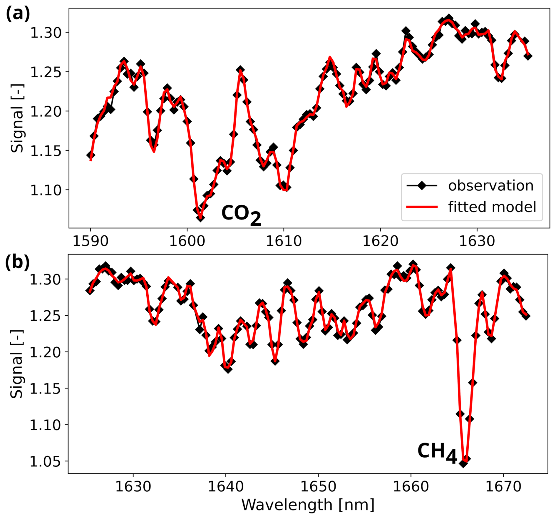
Figure B1 Example fits for the two fit windows used in the WFM-DOAS retrieval: (a) CO₂ and (b) CH₄ fit window. The black diamonds denote the measurement, and the solid red line denotes the fitted model.

Then, the CH₄ column anomalies are computed from the retrieved PSFs as follows:

$$\begin{array}{}\text{(B1)}& \mathrm{\Delta }{V}_{{\mathrm{CH}}_{\mathrm{4}}}=\left({\displaystyle \frac{{\mathrm{PSF}}_{\mathrm{ratio}}}{\stackrel{\mathrm{‾}}{{\mathrm{PSF}}_{\mathrm{ratio}}}}}-\mathrm{1}\right)\cdot {\mathrm{CH}}_{\mathrm{4}}^{\mathrm{abs}\mathrm{col}}\cdot \mathrm{cf},\end{array}$$

where

$$\begin{array}{}\text{(B2)}& {\mathrm{PSF}}_{\mathrm{ratio}}={\displaystyle \frac{{\mathrm{PSF}}_{{\mathrm{CH}}_{\mathrm{4}}}}{{\mathrm{PSF}}_{{\mathrm{CO}}_{\mathrm{2}}}}}.\end{array}$$

PSF_ratio is the unitless ratio of the two retrieved PSFs for CH₄ and CO₂, which is also called the proxy method (Krings et al., 2011, 2013); $\mathrm{\Delta }{V}_{{\mathrm{CH}}_{\mathrm{4}}}$ is the CH₄ column anomaly in $\mathrm{molec}.{\mathrm{cm}}^{-\mathrm{2}}$ (for visualization purposes displayed as % relative to the given background column); cf is a unitless conversion factor (see Appendix B3); ${\mathrm{CH}}_{\mathrm{4}}^{\mathrm{abs}\mathrm{col}}$ is the assumed background column of CH₄ in $\mathrm{molec}.{\mathrm{cm}}^{-\mathrm{2}}$ as used in the RTM simulation; and $\stackrel{\mathrm{‾}}{{\mathrm{PSF}}_{\mathrm{ratio}}}$ denotes a normalization process using observations from the local background (see Sect. 2.4).

As an example, a PSF for CH₄ (${\mathrm{PSF}}_{{\mathrm{CH}}_{\mathrm{4}}}$) of larger than 1 would, compared to the modelled background radiances, indicate more CH₄ in the measured spectrum (and thus in the atmosphere) due to an emission plume and vice versa. However, the absorption depth in a measurement is not only determined by the amount of gases but also by other effects, such as variations in SZA, surface elevation, flight altitude, or aerosol composition, which might not be modelled accurately. These effects lead to a light path error, which affects the PSFs of CH₄ and CO₂ in a similar way due to their spectral proximity. Using the proxy method as indicated in Eq. (B2), which is only possible if there are no major variations in the atmospheric CO₂ concentration field expected, significantly reduces these apparent column variations due to light path errors (Krings et al., 2013, 2011). Another important step is the normalization by the local background, indicated by $\stackrel{\mathrm{‾}}{{\mathrm{PSF}}_{\mathrm{ratio}}}$, and the consideration of the conversion factor before obtaining the CH₄ column anomalies in $\mathrm{molec}.{\mathrm{cm}}^{-\mathrm{2}}$ (or better suited for visualization purposes in %) used during the cross-sectional flux method (Sect. 2.4).

B2 Errors of the CH₄ column anomalies

Previous sensitivity studies have shown (Borchardt et al., 2021; Krautwurst et al., 2021; Krings et al., 2011) that false assumptions in the input parameters for the RTM simulations can cause significant systematic errors in the retrieved single columns or the PSFs of CH₄ and CO₂. Most of these systematic errors are related to light path errors and are thus significantly reduced by the proxy method as described in Sect. B1. Remaining systemic errors (e.g. a changing SZA or a constant offset caused by an inaccurate CO₂ profile, temperature, or aerosol profiles) either vary smoothly with time or are approximately constant over the measurement area. These effects are therefore corrected by the additional normalization with observations outside of a plume. Exceptions could be changes in surface elevation and surface spectral reflectance, which can occur pseudo-randomly and over short distances (see Krautwurst et al., 2021, for details). Additionally, potentially co-emitted CO₂ from landfills affect the proxy method. Krautwurst et al. (2017) have shown that the reduction on the CH₄ anomalies could be around 5 % on average. However, this effect is not considered further here. The sensitivity of the retrieval to parameters for the Madrid flight is summarized in Table B2 and could potentially lead to a remaining systematic offset of the retrieved CH₄ column anomalies of around 0.14 % after correction by the conversion factor (0.763, Krings et al., 2011) resulting from the basic scenario used in Table B2.

Table B2 Sensitivity of the retrieved PSFs to the input parameters for the RTM simulations according to expected variations during the flight on 4 August 2022. The deviations for the PSFs of CH₄, CO₂, and the ratio CH₄ over CO₂ are given relative to the background column. The parameters for the basic scenario used during the retrieval are given in Table B1 using a surface elevation of 0.734 km. Not all values deviate symmetrically around 0 %; therefore, the worst-case scenario is always selected.

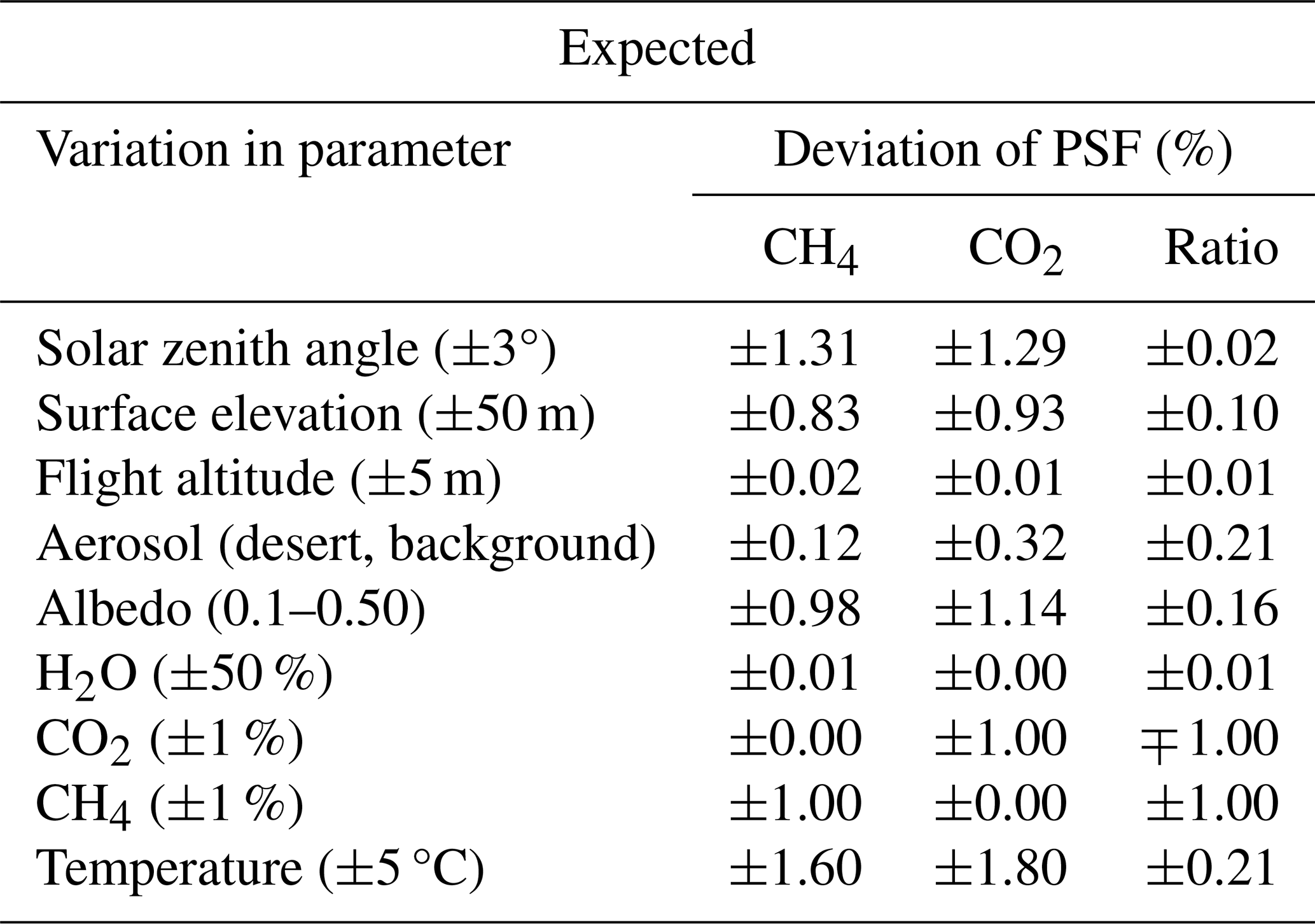
In addition to the systematic effects described above, random effects such as measurement noise produce random column errors. They are not separated further and are estimated together as the single-measurement precision, which is directly computed from the retrieved CH₄ column anomalies outside of the plume (e.g. as done in McLinden et al., 2024; Chulakadabba et al., 2023; Borchardt et al., 2021; Krautwurst et al., 2021; Krings et al., 2013). Moreover, the measurement precision can cover some of the remaining small-scale systematic offsets. For Madrid's landfill flight, it has been estimated to be ∼ 0.4 %. This is slightly worse than that of its precursor instrument MAMAP (see Sect. 2.1.2) and possibly related to the coarser spectral sampling (∼ 3 to 4 pixels vs. ∼ 10 pixels). However, this is compensated by simultaneously acquiring 28 observations in the across-flight direction for a swath width of ∼ 3 km at a flight altitude of ∼ 7.7 $\mathrm{km}\mathrm{a}.\mathrm{g}.\mathrm{l}$.

B3 Averaging kernels and conversion factor

An important parameter of the WFM-DOAS retrieval applied to MAMAP2DL observations is the so-called averaging kernel (AK). It describes the sensitivity of the retrieval to CH₄ column changes at different altitude levels. It is computed by retrieving the CH₄ column from simulated measurements in which the CH₄ concentration at various altitude levels has been perturbed. Figure B2 shows the AK based on a RTM simulation mimicking the atmospheric and geometrical conditions during the flight over Madrid as used in Sect. B1 for analysis of the MAMAP2DL observations.

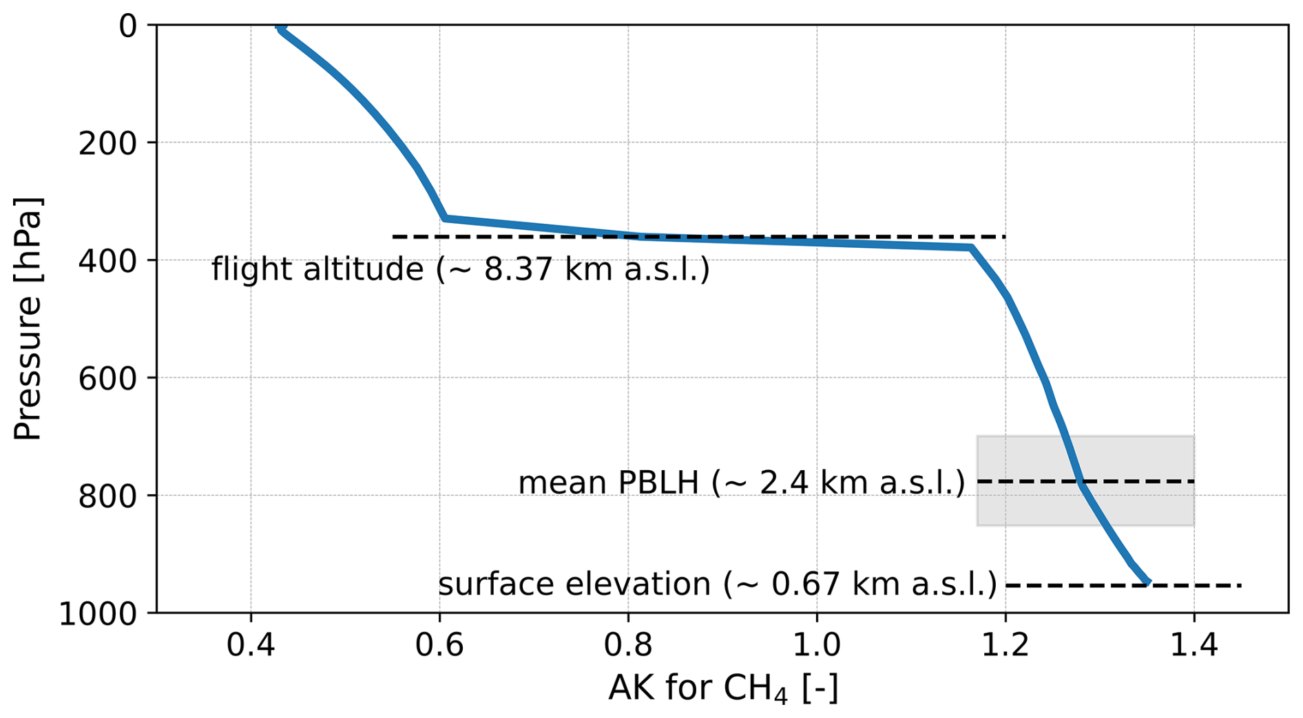
Figure B2 Averaging kernel (AK) of CH₄ for the atmospheric and geometrical conditions as encountered during the Madrid flight for MAMAP2DL. The step in the profile at 8.37 $\mathrm{km}\mathrm{a}.\mathrm{s}.\mathrm{l}.$ (or 7.7 $\mathrm{km}\mathrm{a}.\mathrm{g}.\mathrm{l}.$) marks the flight level of the aircraft. The shaded area of the BLH represents the growth and uncertainty of the BLH during the remote sensing flight according to ERA5 and measured vertical profiles (also see Appendix D2).

An AK of unity at a certain altitude or pressure level would indicate that the retrieval is able to retrieve the perturbed CH₄ concentration correctly. However, due to the measurement geometry, the retrieval overestimates CH₄ changes below the aircraft close to the surface. This effect is related to the light path in the atmosphere. An idealized light beam covers the air masses below the aircraft twice before reaching the sensor, leading to apparent enhanced absorption by CH₄. This effect must be corrected for; otherwise, the retrieval would overestimate potential enhancements below the aircraft.

Assuming that observed variations in the CH₄ column originate from air masses inside the BL, a conversion factor cf is computed as the mean of the averaging kernels ${\stackrel{\mathrm{‾}}{\mathrm{AK}}}_{\mathrm{below}}$ within the BL and then applied in Eq. (B1) for the computation of the column anomaly:

$$\begin{array}{}\text{(B3)}& \mathrm{cf}={\displaystyle \frac{\mathrm{1}}{{\stackrel{\mathrm{‾}}{\mathrm{AK}}}_{\mathrm{below}}}}.\end{array}$$

The altitude-resolved AK(z) is defined as the variation in the retrieved total CH₄ column ∂V_retrieved as a result of a perturbation of the true CH₄ subcolumn ∂v_true(z_j) at altitude z_j (Krings et al., 2011):

$$\begin{array}{}\text{(B4)}& \mathrm{AK}\left(z_j\right)={\displaystyle \frac{\partial V_{\mathrm{retrieved}}}{\partial v_{\mathrm{true}}\left(z_j\right)}}.\end{array}$$

The conversion factor cf for the Madrid flight is 0.763 for an average BLH of 2.4 $\mathrm{km}\mathrm{a}.\mathrm{s}.\mathrm{l}.$, as encountered during the remote sensing flight. Computing the BLH as described in Appendix D2 indicates an increase in the BLH at the position and time of the different flight legs from approx. 1.9 to 2.7 $\mathrm{km}\mathrm{a}.\mathrm{s}.\mathrm{l}$. Considering the given uncertainty of the BLH estimate additionally would lead to an error in the estimated conversion factor of 1.2 %.

B4 Orthorectification

In order to correctly deduce source positions of the CH₄ emission plumes across the two landfills, the CH₄ anomaly maps from MAMAP2DL have to be accurately projected on the ground. An important parameter for this procedure is the attitude information of the aircraft (pitch, roll, and yaw), which defines the line of sight of the instrument. Moreover, the aircraft's flight altitude and the surface elevation at the position of the projected ground scene, in combination with the viewing angle of the instrument, determine the across-leg ground scene size and thus the width of the entire swath and, finally, the aircraft position itself. The position and attitude data (pitch, roll, yaw, flight altitude, location) are provided by the BAHAMAS system introduced in Sect. 2.1.4 at a resolution of 10 Hz. Topography data are derived from the Shuttle Radar Topography Mission (SRTM; Farr et al., 2007) digital elevation model (DEM) also used for the estimate of the surface elevation applied in the RTMs in Appendix B1. Next, the orthorectification is performed along the lines as described in Schoenhardt et al. (2015).

As the main RGB imagery source, we use Google Earth data, overlaid with the CH₄ column anomaly maps (as KMZ files; see Fig. 5). Therefore, the accuracy of the orthorectification is validated against Google Earth imagery. Coincidentally, at least some of the Google Earth images of Madrid were taken in August 2022, which is in the same month as the measurements were acquired. Therefore, we assume that the state of the landfill during the overflight on 4 August is very similar to that shown in the Google Earth images. For the validation process, we use high-resolution-intensity (not spatially binned) maps of the measured on-chip signal strength around 1.6 µm with a spatial resolution of ∼ 8.5 m in the along-flight direction, as they mimic to a certain degree the surface properties and structures seen in the Google Earth RBG maps. The deviations (or better gradients) of distinct features such as rivers or streets are then used to verify the accuracy of the orthorectification. In the along-flight direction, the accuracy is better than ∼ 20 m, whereas, in the across-flight direction, it is determined by the coarse spatial resolution of ∼ 110 m. Overall, we estimate an accuracy of the column anomaly maps of better than 110 m, or around one ground scene, for the Madrid dataset, which is generally limited by the final ground scene size.

Appendix C: CHARM-F retrieval

C1 Retrieval and weighting function

The quantity that is independently measured by CHARM-F is the differential absorption optical depth (DAOD; Δτ), calculated from the received signals with

$$\begin{array}{}\text{(C1)}& \mathrm{\Delta }\mathit{\tau }={\displaystyle \frac{\mathrm{1}}{\mathrm{2}}}\ln \left({\displaystyle \frac{S_{\mathrm{off}}/E_{\mathrm{off}}}{S_{\mathrm{on}}/E_{\mathrm{on}}}}\right).\end{array}$$

S_on and S_off are backscattered signals and E_on and E_off are internal energy reference measurements at the online and offline wavelength, respectively. Δτ, on the other hand, can also be described in terms of the molecular absorption cross-section at both wavelengths (σ_on and σ_off) and the number density $n_{{\mathrm{CH}}_{\mathrm{4}}}$ or the dry-air mixing ratio of methane $r_{{\mathrm{CH}}_{\mathrm{4}}}$.

$$\begin{array}{}\text{(C2)}& {\displaystyle }\mathrm{\Delta }\mathit{\tau }& {\displaystyle }=\underset{h_{\mathrm{0}}}{\overset{h_{\mathrm{1}}}{\int }}{n}_{{\mathrm{CH}}_{\mathrm{4}}}\underset{=\mathrm{\Delta }\mathit{\sigma }}{\underbrace{({\mathit{\sigma }}_{\mathrm{on}}-{\mathit{\sigma }}_{\mathrm{off}})}}\mathrm{d}h,\text{(C3)}& {\displaystyle }& {\displaystyle }=\underset{h_{\mathrm{0}}}{\overset{h_{\mathrm{1}}}{\int }}{\displaystyle \frac{r_{{\mathrm{CH}}_{\mathrm{4}}}}{\left(\mathrm{1}+r_{{\mathrm{H}}_{\mathrm{2}}\mathrm{O}}\right)}}\cdot n_{\mathrm{air}}\cdot \mathrm{\Delta }\mathit{\sigma }\mathrm{d}h.\end{array}$$

The integral runs over the air column between the aircraft (h₁) and the ground (h₀). In Eq. (C3), the number density of greenhouse gas molecules is expressed in terms of the number density of air molecules n_air and the dry-air molar mixing ratio of the greenhouse gas species, while also accounting for the dry-air molar mixing ratio of water,

$$\begin{array}{}\text{(C4)}& n_{\mathrm{air}}=\left(\mathrm{1}+r_{{\mathrm{H}}_{\mathrm{2}}\mathrm{O}}\right)\cdot n_{\mathrm{dry}\mathrm{air}}.\end{array}$$

Using the general gas equation $\left(n_{\mathrm{air}}=\frac{p}{k_{\mathrm{B}}\cdot T}\right)$, n_air can be expressed in terms of pressure p and temperature T. Furthermore, the integral over altitude can be transformed into a pressure integral $\left(\mathrm{d}h=\frac{\mathrm{d}h}{\mathrm{d}p}\cdot \mathrm{d}p=-\frac{k_{\mathrm{B}}\cdot N_{\mathrm{A}}\cdot T}{p\cdot M_{\mathrm{air}}\cdot g}\mathrm{d}p\right)$,

$$\begin{array}{}\text{(C5)}& \mathrm{\Delta }\mathit{\tau }=\underset{p_{\mathrm{1}}}{\overset{p_{\mathrm{0}}}{\int }}{\displaystyle \frac{r_{{\mathrm{CH}}_{\mathrm{4}}}\cdot N_{\mathrm{A}}}{\left(\mathrm{1}+r_{{\mathrm{H}}_{\mathrm{2}}\mathrm{O}}\right)\cdot M_{\mathrm{air}}\cdot g}}\cdot \mathrm{\Delta }\mathit{\sigma }\mathrm{d}p.\end{array}$$

Here, k_B is the Boltzmann constant, N_A is the Avogadro constant, g is the gravitational acceleration, and M_air is the average molar mass of air. Next, molar mass is expressed as molecular mass $\left(m_{\mathrm{air}}=\frac{M_{\mathrm{air}}}{N_{\mathrm{A}}}\right)$, and dry air is discriminated from water vapour.

$$\begin{array}{}\text{(C6)}& {\displaystyle }\mathrm{\Delta }\mathit{\tau }& {\displaystyle }=\underset{p_{\mathrm{1}}}{\overset{p_{\mathrm{0}}}{\int }}{\displaystyle \frac{r_{{\mathrm{CH}}_{\mathrm{4}}}}{\left(\mathrm{1}+r_{{\mathrm{H}}_{\mathrm{2}}\mathrm{O}}\right)}}\cdot {\displaystyle \frac{\mathrm{\Delta }\mathit{\sigma }}{\underset{=\frac{m_{\mathrm{dry}\mathrm{air}}+r_{{\mathrm{H}}_{\mathrm{2}}\mathrm{O}}{m}_{{\mathrm{H}}_{\mathrm{2}}\mathrm{O}}}{\mathrm{1}+r_{{\mathrm{H}}_{\mathrm{2}}\mathrm{O}}}}{\underbrace{m_{\mathrm{air}}}}\cdot g}}\mathrm{d}p,\text{(C7)}& {\displaystyle }& {\displaystyle }=\underset{p_{\mathrm{1}}}{\overset{p_{\mathrm{0}}}{\int }}{\displaystyle \frac{r_{{\mathrm{CH}}_{\mathrm{4}}}}{\left(m_{\mathrm{dry}\mathrm{air}}+r_{{\mathrm{H}}_{\mathrm{2}}\mathrm{O}}\cdot m_{{\mathrm{H}}_{\mathrm{2}}\mathrm{O}}\right)}}\cdot {\displaystyle \frac{\mathrm{\Delta }\mathit{\sigma }}{g}}\mathrm{d}p.\end{array}$$

Finally, $r_{{\mathrm{CH}}_{\mathrm{4}}}$ is pulled out of the integral by replacement with a (weighted) column average XCH₄, which is thus defined:

$$\begin{array}{}\text{(C8)}& {\displaystyle }\mathrm{\Delta }\mathit{\tau }& {\displaystyle }=X{\mathrm{CH}}_{\mathrm{4}}\underset{p_{\mathrm{1}}}{\overset{p_{\mathrm{0}}}{\int }}{\displaystyle \frac{{\mathit{\sigma }}_{\mathrm{on}}\left(p,T\right)-{\mathit{\sigma }}_{\mathrm{off}}\left(p,T\right)}{g\left(m_{\mathrm{dry}\mathrm{air}}+r_{{\mathrm{H}}_{\mathrm{2}}\mathrm{O}}\cdot m_{{\mathrm{H}}_{\mathrm{2}}\mathrm{O}}\right)}}\mathrm{d}p,\text{(C9)}& {\displaystyle }& {\displaystyle }=X{\mathrm{CH}}_{\mathrm{4}}\underset{p_{\mathrm{1}}}{\overset{p_{\mathrm{0}}}{\int }}W(p,T)\mathrm{d}p.\end{array}$$

The quotient remaining in the integral is the so-called weighting function

$$\begin{array}{}\text{(C10)}& W\left(p,T\right)={\displaystyle \frac{{\mathit{\sigma }}_{\mathrm{on}}\left(p,T\right)-{\mathit{\sigma }}_{\mathrm{off}}\left(p,T\right)}{g\cdot \left(m_{\mathrm{dry}\mathrm{air}}+m_{{\mathrm{H}}_{\mathrm{2}}\mathrm{O}}\cdot r_{{\mathrm{H}}_{\mathrm{2}}\mathrm{O}}\right)}},\end{array}$$

which carries the terms that are pressure-/altitude-dependent but known to some degree. In the standard data analysis routines of CHARM-F, the absorption cross-sections are calculated based on the spectroscopic datasets GEISA20 and Vasilchenko (Delahaye et al., 2021; Vasilchenko et al., 2023), and the state of the atmosphere (vertical structure at measurement location) is extracted from the ECMWF Integrated Forecasting System (IFS).

The partial-column weighted-average molar mixing ratio is therefore described by

$$\begin{array}{}\text{(C11)}& X{\mathrm{CH}}_{\mathrm{4}}={\displaystyle \frac{\mathrm{\Delta }\mathit{\tau }}{{\int }_{p_{\mathrm{1}}}^{p_{\mathrm{0}}}W\left(p,T\right)\mathrm{d}p}}.\end{array}$$

C2 Column anomalies from CHARM-F measurements

This subsection describes the details of how we convert XCH₄, as measured by CHARM-F, into a column anomaly of the dry-air CH₄ molar mixing ratio for the total column. The reference for the calculation of anomaly is the methane concentration from the Copernicus Atmosphere Monitoring Service (CAMS) global inversion model (CAMS, 2023). Based on the dry-air molar mixing ratio from CAMS ($r_{{\mathrm{CH}}_{\mathrm{4}},\mathrm{CAMS}}$), we calculate a column-averaged molar mixing ratio between surface (sfc) and flight altitude (flh), using the number density of air molecules from CAMS as weight n_air:

$$\begin{array}{}\text{(C12)}& X{{\mathrm{CH}}_{\mathrm{4}}}_{\mathrm{CAMS}}={\displaystyle \frac{{\int }_{\mathrm{sfc}}^{\mathrm{flh}}{r}_{{\mathrm{CH}}_{\mathrm{4}},\mathrm{CAMS}}\cdot n_{\mathrm{air}}\mathrm{d}z}{{\int }_{\mathrm{sfc}}^{\mathrm{flh}}{n}_{\mathrm{air}}\mathrm{d}z}}.\end{array}$$

On this basis, the partial-column anomaly A_pc is calculated.

Due to the temperature and pressure dependence of the spectroscopic properties of methane, $X{{\mathrm{CH}}_{\mathrm{4}}}_{\text{CHARM-F}}$ and $X{{\mathrm{CH}}_{\mathrm{4}}}_{\mathrm{CAMS}}$ are weighted somewhat differently along the column (see Fig. C1). Nevertheless, in the hypothetical case, where methane is homogeneously distributed along the surveyed column, they give the exact same result by definition of the weighting function. To compensate for this small bias (few percent), which only affects the anomalous part of the column concentration, based on the CHARM-F weighting function W(p,T), we calculate a correction factor:

$$\begin{array}{}\text{(C13)}& C_W={\displaystyle \frac{\frac{{\int }_{\mathrm{sfc}}^{\mathrm{flh}}W\left(p,T\right)n_{\mathrm{air}}\mathrm{d}z}{{\int }_{\mathrm{sfc}}^{\mathrm{flh}}{n}_{\mathrm{air}}\mathrm{d}z}}{\frac{{\int }_{\mathrm{sfc}}^{\mathrm{blh}}W\left(p,T\right)n_{\mathrm{air}}\mathrm{d}z}{{\int }_{\mathrm{sfc}}^{\mathrm{blh}}{n}_{\mathrm{air}}\mathrm{d}z}}}.\end{array}$$

Here, we assume that methane plumes from a nearby source at the surface lead to a mole fraction enhancement only below the top of the atmospheric BL. No enhancement is expected within the free troposphere up to the flight altitude (flh). C_W quantifies the ratio between how a homogeneously distributed methane enhancement would be perceived by CHARM-F versus an enhancement that is also homogeneous but restricted to the BL.

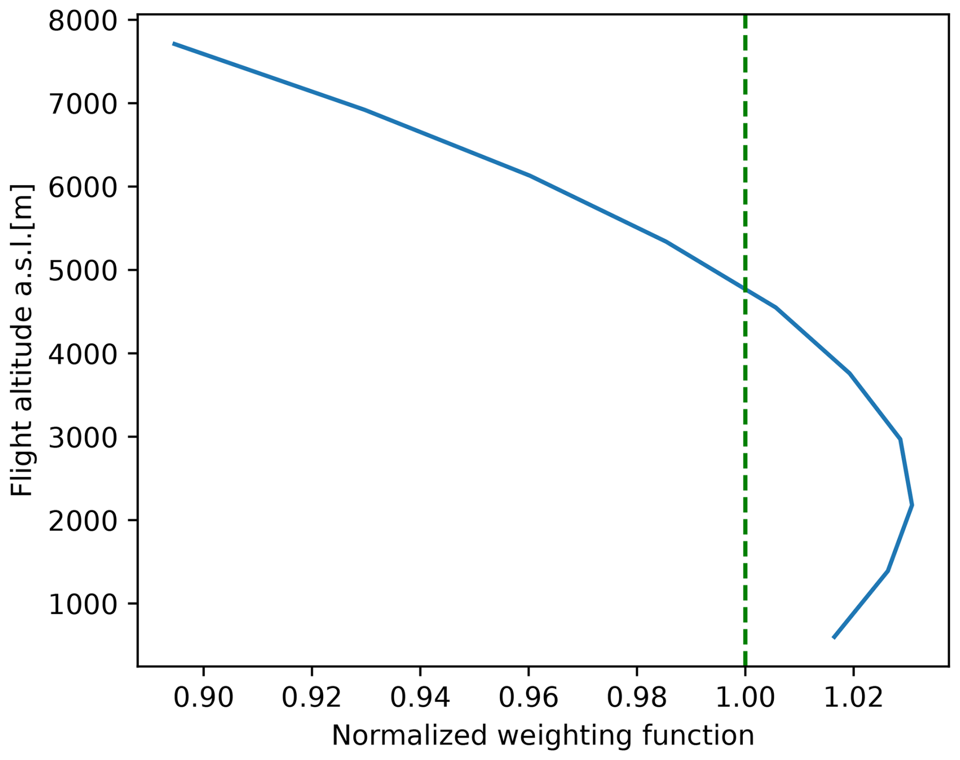
Figure C1 Typical altitude dependency of the CHARM-F weighting function for methane. The weighting function is normalized to the particle-number-averaged value of the column between the ground and the flight altitude of about 8 km. The dashed green line indicates the unity weighting used for the CAMS reference column concentration.

The partial-column anomaly for the column below the aircraft can therefore be calculated as follows:

$$\begin{array}{}\text{(C14)}& A_{\mathrm{pc}}=C_W\cdot {\displaystyle \frac{X{\mathrm{CH}}_{\mathrm{4}}-X{{\mathrm{CH}}_{\mathrm{4}}}_{\mathrm{CAMS}}}{X{{\mathrm{CH}}_{\mathrm{4}}}_{\mathrm{CAMS}}}}.\end{array}$$

Finally, the column from the aircraft to the top of the atmosphere (toa) also has to be considered. That region, where the anomaly is zero by definition, is combined with the column below by averaging, using the particle number density of air molecules as weight:

$$\begin{array}{}\text{(C15)}& A_{\mathrm{tc}}={\displaystyle \frac{A_{\mathrm{pc}}\cdot {\int }_{\mathrm{sfc}}^{\mathrm{flh}}{n}_{\mathrm{air}}\mathrm{d}z}{{\int }_{\mathrm{sfc}}^{\mathrm{toa}}{n}_{\mathrm{air}}\mathrm{d}z}}.\end{array}$$

Thus, A_tc is the closest approximation of the CH₄ anomaly in terms of mole fraction for the total-column along-flight tracks, comparing CHARM-F measurements with CAMS reanalysis data as reference.

C3 Uncertainties of CHARM-F measurements

The measurement uncertainties of XCH₄ retrieved with CHARM-F can be categorized into statistical and systematic uncertainties. Statistical uncertainties are introduced through the measurement of DAOD or, more precisely, the measurement of the four signal intensities that contribute to DAOD. These are associated with a certain degree of noise, largely independent between individual laser pulses. The main noise sources are photon statistics, detector noise, and speckle noise (Ehret et al., 2008). The exact magnitude can be estimated from the system parameters or directly determined from measurement statistics. The influence of these uncertainties can be reduced by averaging multiple pulse pairs. Such statistical uncertainties can be characterized with an Allan deviation (Allan, 1966) plot, as shown in Fig. C2. For an individual double-pulse measurement, the standard deviation is about 100 ppb or 5 %. Averaging multiple measurements reduces the uncertainty with an inverse-square-root law, as expected, at until about 1 s of averaging. At this point, the Allan deviation diverges from this noise-only expectation, which can be explained by actual gradients in the form of the observed methane plumes. Residual uncertainties from systematic drifts or offsets have to be addressed using a different strategy.

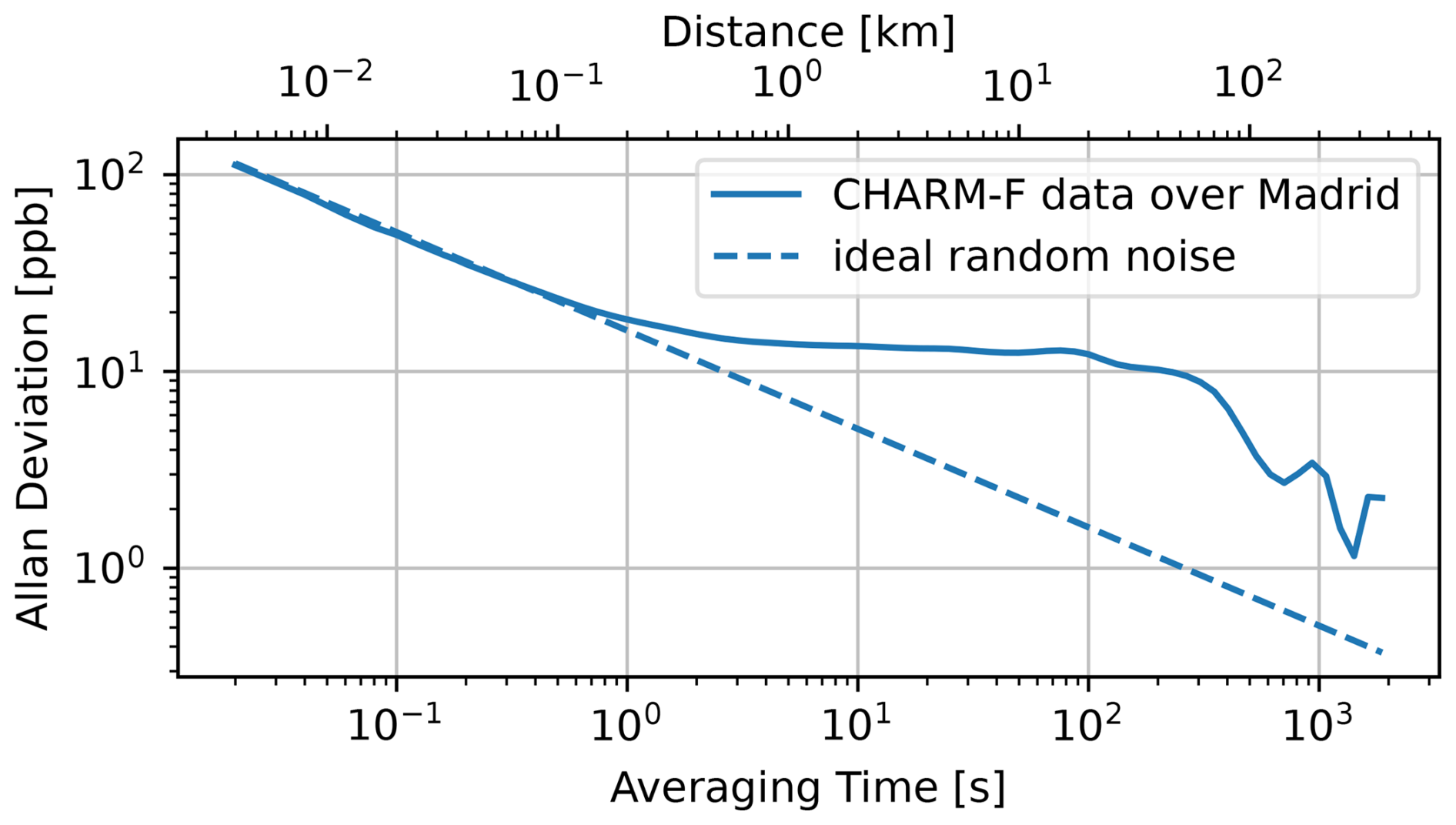
Figure C2 Allan deviation plot of the CHARM-F measurements over the Madrid landfills. In the case of pure ideal noise, the scatter reduces from single-pulse-pair measurements with 1 over the square root of the number of measurements that are averaged. Deviations indicate either drifts or, as in this case, mostly real methane gradients.

Systematic uncertainties are related to inaccurate knowledge or deviation of certain system or meteorological parameters from the design/assumed values. These deviations typically change over time at very slow rates of the order of minutes to hours and are therefore highly correlated between individual pulse pairs. Systematic uncertainties arise from various sources. These include small misalignments in the optical setup, which could cause unequal clipping of light between the online and offline pulses in the receiver. Additional factors contributing to uncertainties are errors in the tuning of the emitted wavelengths, spectroscopic inaccuracies, and discrepancies between the numerical weather simulation model and the actual atmospheric conditions during measurement, which impact the calculation of the weighting function (Ehret et al., 2008).

In order to estimate relevant systematic uncertainties for our measurements, we define a background region, southeast of the landfills and the city of Madrid. The region was chosen such that the aircraft typically stays within that region for about 100 s or 5000 individual measurements (orange track segments in Fig. C3). This length/duration is comparable to the typical plume or background regions used for the flux measurements. For each overpass of the background region, the average partial-column XCH₄ is computed, resulting in a residual scatter of 4 ppb or 0.2 %. From extrapolating the random-noise model in the Allan deviation plot, 2 ppb or 0.1 % is expected. We conclude that, on the timescales that are relevant for our measurements, systematic effects lead to a doubling of the errors that would be expected from random noise only.

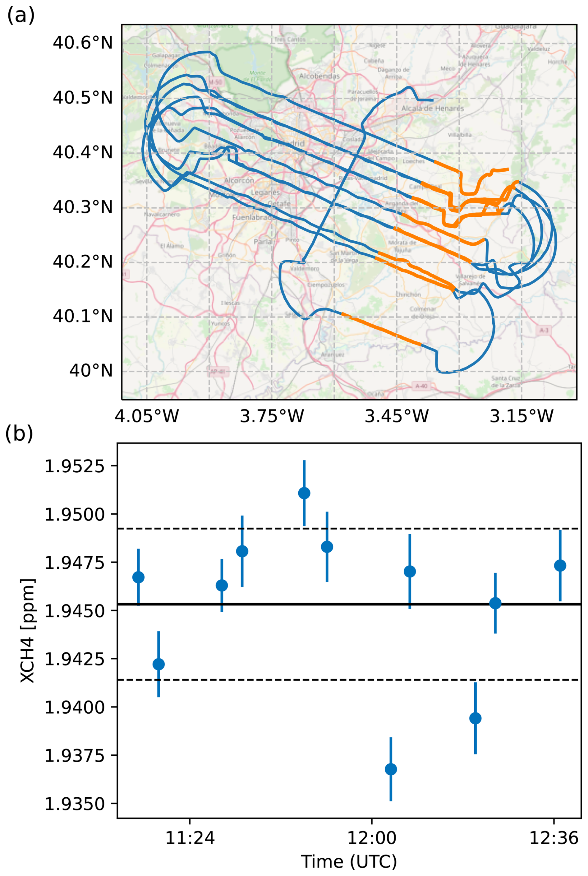
Figure C3 Uncertainties of the CHARM-F column concentration background, averaged over 100 s background segments. The flight track segments that were used for the background uncertainty study are shown in orange (a). The average values and statistical errors XCH₄ for these segments are shown in panel (b), together with the overall mean value and standard deviation band, drawn as solid and dashed lines, respectively. Base map data © OpenStreetMap contributors 2024. Distributed under the Open Data Commons Open Database License (ODbL) 1.0. Tiles accessed using Cartopy.

Appendix D: Validation of ECMWF ERA5 data by on-board aircraft measurements

D1 Validation of ERA5 wind data

In order to confirm that the wind parameters, which are relevant for our flux or emission rate estimates, are correctly modelled in ECMWF ERA5, we compare them to on-board in situ wind measurements on HALO from BAHAMAS (see Sect. 2.1.4). ERA5 data have been interpolated and evaluated along the flight track in space and time. The on-board measurements have been smoothed with a 30 s Gaussian kernel to reduce fluctuations from turbulence, which is on a scale far below the resolution of ERA5. The ERA5 model matches the BAHAMAS measurements very well over longer time frames, especially when neglecting the small-scale turbulence still visible in Fig. D1. This is particularly valid for the part of the flight within the BL (grey region), where the plume is located. The averaged difference between model and measurement for the wind speed and wind direction is 0.05 m s⁻¹ and 0.8° in the BL (averages are actually quite independent from the applied smoothing kernel). The only caveat is that the time period for which the good match can be demonstrated is up to around 2 h after the start of the remote sensing section of the flight. Therefore, a similarly good match between model prediction and actual wind situation within the BL also has to be assumed for earlier times without explicit proof. The significantly larger mismatch between ERA5 and the measured winds in some segments of the flight at earlier times (not within the BL) can most likely be explained with strong wind shear in a thin layer, exactly at the flight altitude during the remote sensing part of the flight, in combination with a relatively coarse vertical resolution of ECMWF there.

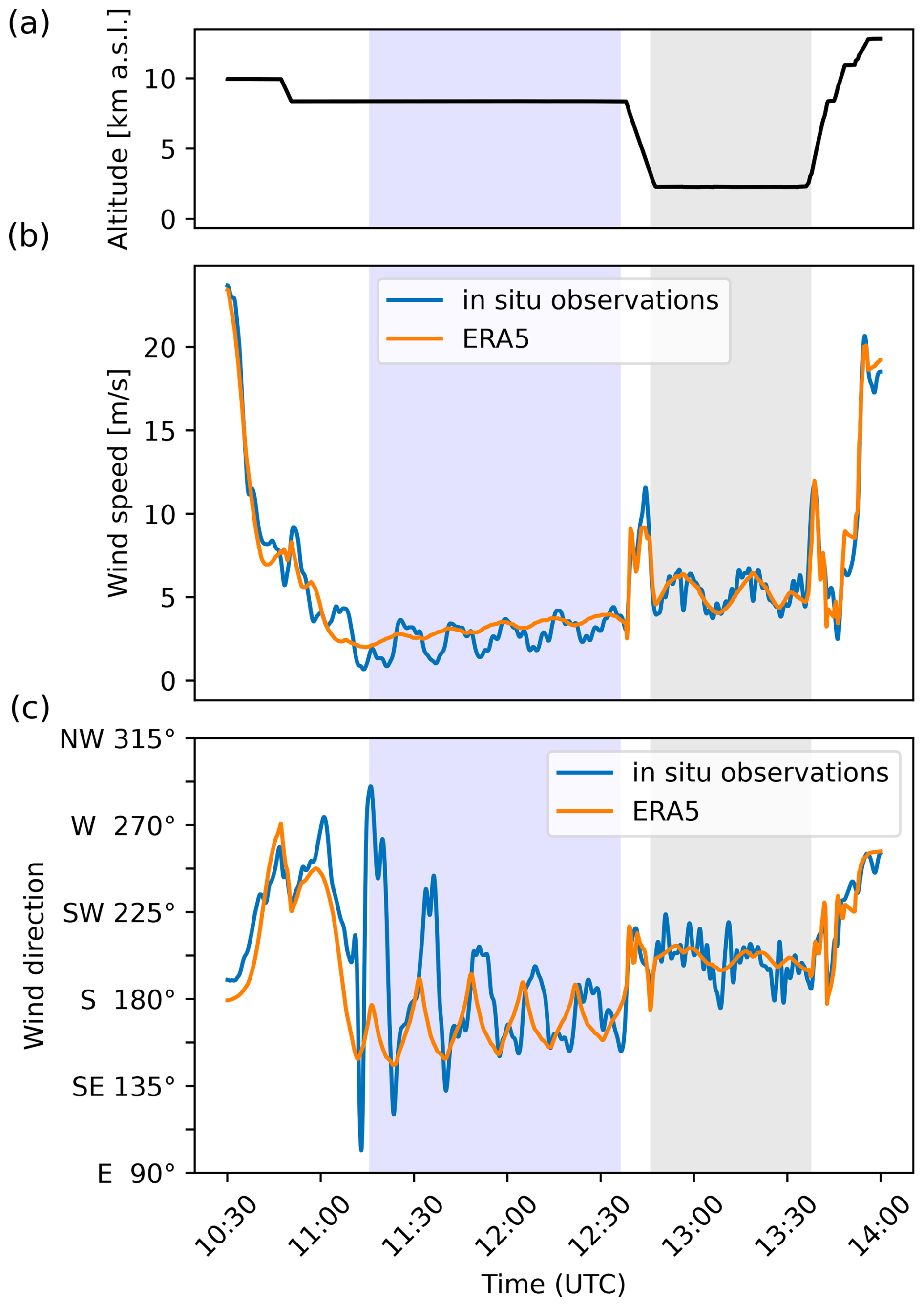
Figure D1 Flight altitude of HALO (a), wind speed (b), and direction (c) as modelled in ECMWF ERA5 vs. actual in situ measurements of BAHAMAS during the HALO flight over Madrid. The section of the flight that took place within the BL is highlighted in grey, and the section for the remote sensing observations is in light blue.

Interestingly, during the descent into the BL (at around 12:45 UTC) and the subsequent ascent around 2 h later, the wind speed peaks at values of up to 10 m s⁻¹ without significant change in wind direction. This indicates a strong vertical gradient in wind speed in the BL in both model and measurement from top of the BL to at least 1.6 $\mathrm{km}\mathrm{a}.\mathrm{g}.\mathrm{l}$. This is actually confirmed by vertical profiles of the wind speed from ERA5 data (Fig. D2a). They show a strong vertical gradient, which is around 2 m s⁻¹ at the ground and increases to 10 m s⁻¹ at the top of BL for 12:00 UTC. Moreover, on that day, the wind speed increases from 10:00 to 14:00 UTC in the BL. The wind direction (Fig. D2b) is relatively stable after 11:00 UTC, with values between 200 and 220°. However, before the stabilization to south-southwest at 11:00 UTC (right before the measurement flight started), the wind had a strong easterly component.

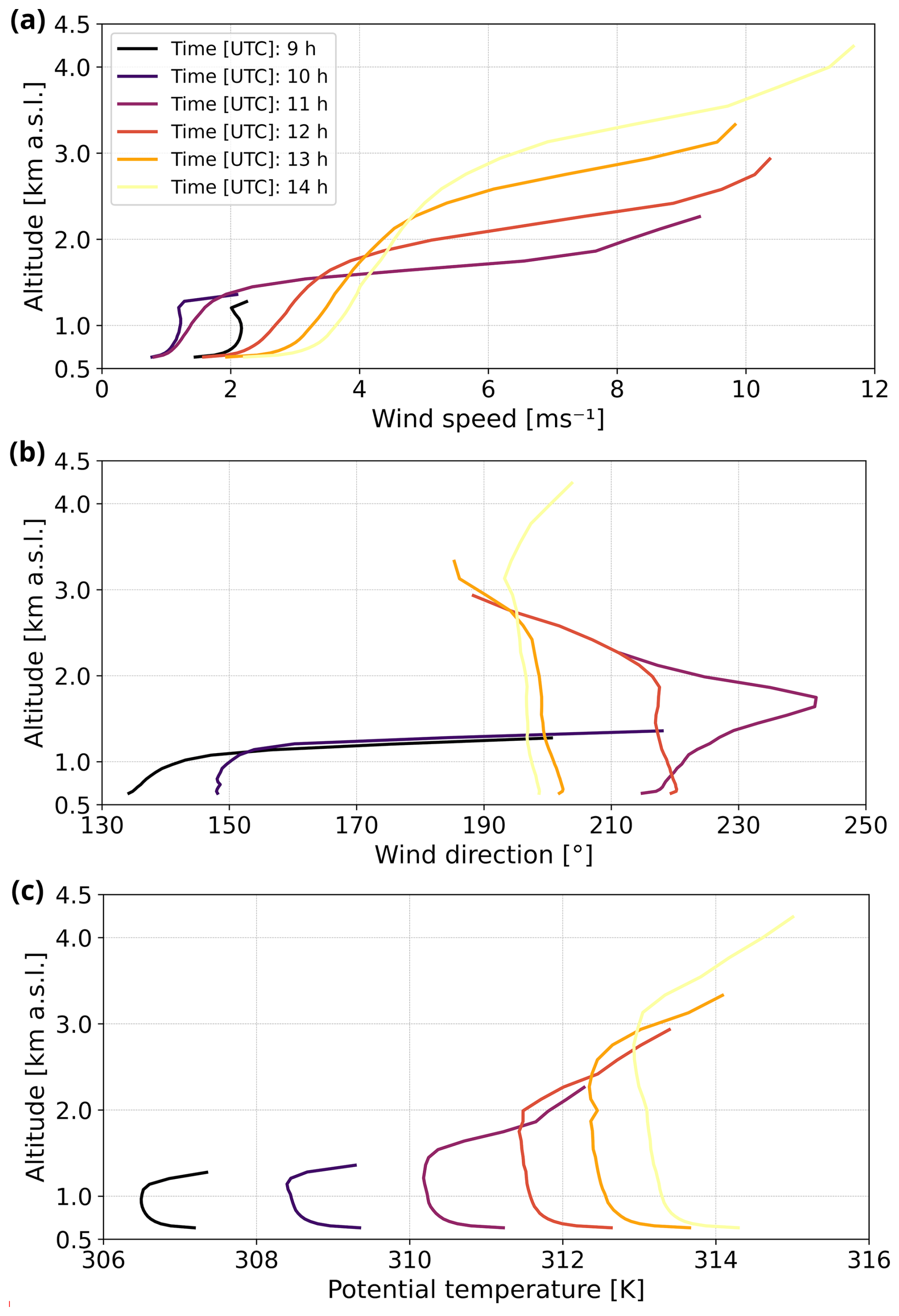
Figure D2 Vertical profiles for wind speed (a), wind direction (b), and potential temperature (c) between 09:00 and 14:00 UTC based on the ECMWF ERA5 model data. The height of the profiles is restricted to the BLH as given in ERA5. The time of the remote sensing overflight was between 11:00 and 12:40 UTC. In situ data collection within the BL was between 12:50 and 13:30 UTC. The profiles are representative for 40.292° N and 3.614° W, which is located between the two landfill complexes.

D2 Validation of ERA5 BLH data

For the BLH, ERA5 shows an increase from ∼ 1.3 $\mathrm{km}\mathrm{a}.\mathrm{s}.\mathrm{l}.$ (0.7 $\mathrm{km}\mathrm{a}.\mathrm{g}.\mathrm{l}.$) to ∼ 4.2 $\mathrm{km}\mathrm{a}.\mathrm{s}.\mathrm{l}.$ (3.6 $\mathrm{km}\mathrm{a}.\mathrm{g}.\mathrm{l}.$) nicely illustrated in the potential temperature profiles for that location and time period (Fig. D2c). To validate ERA5's BLH, we compare it to measured potential temperature profiles during the descent and ascent at 12:45 UTC (40.345° N, 3.010° W) and 13:40 UTC (40.322° N, 3.745° W), respectively, at the respective locations. The descent took place over a more hilly environment approx. 50 km east of the landfills, and the ascent was right over the city of Madrid 12 km west of the landfills.

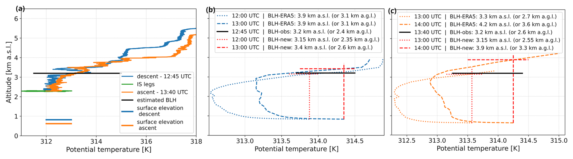
Figure D3 Comparison between HALO in situ measurements and ERA5 model data. The vertical profiles of potential temperature for the descent at 12:45 UTC (40.345° N, 3.010° W) and the ascent at 13:40 UTC (40.322° N, 3.745° W) as measured by BAHAMAS aboard HALO are shown in panel (a). The solid black horizontal line marks the BLH, estimated from these profiles to be 3.2 $\mathrm{km}\mathrm{a}.\mathrm{s}.\mathrm{l}.$, in all panels. Blue marks the profile during descent; the relevant ERA5 model profiles at that location and those times (12:00 UTC, dotted; 13:00 UTC, dashed) are then given in panel (b). Orange marks the profile during ascent; the relevant ERA5 model profiles at that location and those times (13:00 UTC, dotted; 14:00 UTC, dashed) are then given in panel (c). Red vertical and horizontal lines mark the newly estimated BLH for each time step in the model based on the method described in the main text. Different line types show different temporal affiliations. BLH values are given in the legends.

Both profiles are shown in Fig. D3a. We estimate the BLH for both profiles to be ∼ 3.2 $\mathrm{km}\mathrm{a}.\mathrm{s}.\mathrm{l}.$ (considering topography would yield 2.4 and 2.6 $\mathrm{km}\mathrm{a}.\mathrm{g}.\mathrm{l}.$ for descent and ascent, respectively) due to the strong increase in potential temperatures at these altitudes. Comparing the BLHs from ERA5 at these positions and times yields significantly and consistently higher BLHs of 700 m relative to sea level (Fig. D3b, c). In order to correct for this discrepancy but also to transfer it to an earlier measurement time, when the remote sensing observations were collected, we use the potential temperature profile from ERA5 and estimate a new BLH. We do that by using the temperature at the surface and then searching for the altitude level where this value is approached for the first time. The assumption behind this is that an air parcel, having a certain potential temperature, rises if the potential temperature is lower in the surrounding air masses and reaches an equilibrium (height) when the potential temperature is similar to its surroundings. This process is indicated in Fig. D3b and c by the vertical red lines for the respective time steps of the model. If the leg, or in this case one profile, is collected in between two time steps, the newly computed BLH is linearly interpolated in time.

For the descending and ascending profiles, this method yields ∼ 3.33 $\mathrm{km}\mathrm{a}.\mathrm{s}.\mathrm{l}.$ (2.53 $\mathrm{km}\mathrm{a}.\mathrm{g}.\mathrm{l}.$) and ∼ 3.65 $\mathrm{km}\mathrm{a}.\mathrm{s}.\mathrm{l}.$ (3.05 $\mathrm{km}\mathrm{a}.\mathrm{g}.\mathrm{l}.$), respectively, which is up to 15 % lower than given directly by ERA5 with regard to $\mathrm{km}\mathrm{a}.\mathrm{s}.\mathrm{l}$. On average, over all leg positions and times, the BLHs decrease by around 17 %, which also leads to a decrease in the computed wind speed of 24 %. As a conservative uncertainty estimate, we assume an error of 20 % in our BLH estimate with respect to its depth relative to the ground. A deeper BL would have a larger error. Applying this to the profiles would lead to absolute errors in the BLH for descent and ascent of 0.5 and 0.6 km, respectively. This uncertainty in BLH translates into a wind speed uncertainty of 0.8 m s⁻¹ (or 20 %) on average for our flight legs. The wind direction is hardly influenced by a change in BLH.

Appendix E: Column and flux comparison MAMAP2DL and CHARM-F

Figure E1 summaries the comparison of cross-sections between MAMAP2DL and CHARM-F.

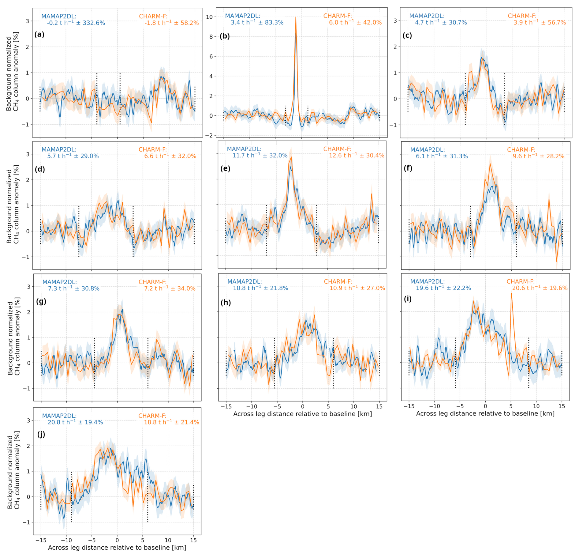
Figure E1 Same as Fig. 6 but for the remaining cross-sectional fluxes of the different legs from MAMAP2DL and CHARM-F observations. The cross-section in Fig. 6 would correspond to panel (g). The order of cross-sections is from upwind (a) to downwind (j). The spike in the CHARM-F column anomalies at ∼ 5 km in panel (i) is an albedo artefact due to retro-reflecting road markings parallel to the flight leg.

Appendix F: Errors of the flux estimates

F1 General error handling

Assuming that the CH₄ emission plumes are well mixed within the BL, major error sources for the cross-sectional flux computation are the wind speed and direction, the random and systematic errors of the retrieved column anomalies from the remote sensing instruments, the boundaries or limits of the background normalization used to compute the real enhancements, and the uncertainty in the estimate of the BLH from ERA5. To compute these errors, we use Gaussian error propagation of Eq. (1)/(2) where possible. All considered sources of uncertainty are summarized in Table F1, and their range is given in Table 1. Error propagation is applied to the error in wind speed (δF_u) and the error in the BLH (δF_blh), which changes the part of the wind profiles over which the average is calculated, and to remaining systematic errors of the columns (δF_col-ac) and of the conversion factor (δF_col-cf). Moreover, the random error of the columns (δF_col-pr) is propagated. However, the single-column precision is additionally divided by $\sqrt{k}$, with k being the number of measurements or ground scenes inside of the plume of one cross-section, taking into account its random nature (see, for example, Appendix C3). The error of the wind direction on the computed flux is considered by varying the direction (α) according to the respective directional uncertainty. The error in the flux is then given by the variation in the computed fluxes. In a similar way, we take into account the error of the background normalization (δF_bg) by computing a set of fluxes based on reasonable variations in the background limits and calculating the standard deviation of their differences from the main flux estimate.

Table F1 Summary of relevant error sources and quantities for the flux computation.

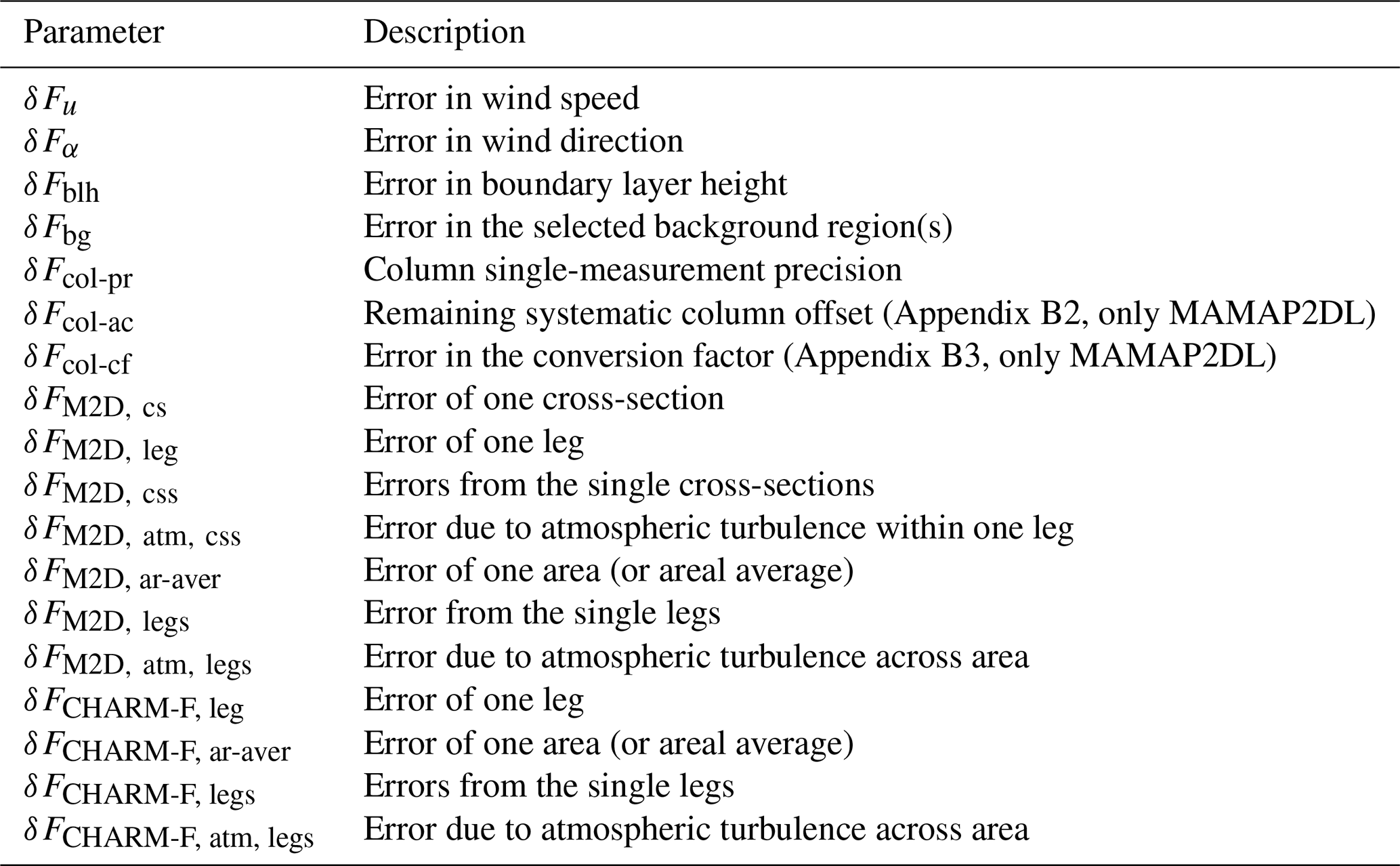
F2 Error handling for MAMAP2DL

In the case of MAMAP2DL, the total error of the flux of one cross-section (δF_M2D, cs) is calculated by root-sum-squaring the error contributions:

$$\begin{array}{}\text{(F1)}& \mathit{\delta }{F}_{\mathrm{M}\mathrm{2}\mathrm{D},\mathrm{cs}}=\sqrt{\begin{array}{rl}{\displaystyle }& {\displaystyle }\mathit{\delta }{F}_u^{\mathrm{2}}+\mathit{\delta }{F}_{\mathit{\alpha }}^{\mathrm{2}}+\mathit{\delta }{F}_{\mathrm{blh}}^{\mathrm{2}}+\mathit{\delta }{F}_{\mathrm{bg}}^{\mathrm{2}}\\ {\displaystyle }+& {\displaystyle }\mathit{\delta }{F}_{\text{col-pr}}^{\mathrm{2}}\left(k\right)+\mathit{\delta }{F}_{\text{col-ac}}^{\mathrm{2}}+\mathit{\delta }{F}_{\text{col-cf}}^{\mathrm{2}}\end{array}}.\end{array}$$

If the emission source is constant, the actual uncertainty of the flux of one cross-section at a certain position is also influenced by atmospheric variability or turbulence in the atmosphere (Krautwurst et al., 2021; Wolff et al., 2021; Krautwurst et al., 2017; Matheou and Bowman, 2016). This is also visible in the imaging data and at this point is not covered by the error δF_M2D, cs (Eq. F1). However, this error component is reduced by taking spatially and/or temporally independent cross-sections. We estimate this factor as 1σ standard deviation (SD) from the cross-sections of one entire MAMAP2DL leg itself:

$$\begin{array}{}\text{(F2)}& \mathit{\delta }{F}_{\mathrm{M}\mathrm{2}\mathrm{D},\mathrm{atm},\mathrm{css}}={\displaystyle \frac{\mathrm{SD}\left(F_{\mathrm{M}\mathrm{2}\mathrm{D},\mathrm{cs},j}\right)}{\sqrt{n_{\mathrm{eff}}}}},\end{array}$$

where n_eff is the number of actual independent cross-sections across a MAMAP2DL flight leg. Additionally, the wind ($\mathit{\delta }{F}_u^{\mathrm{2}}$ and $\mathit{\delta }{F}_{\mathit{\alpha }}^{\mathrm{2}}$), BLH ($\mathit{\delta }{F}_{\mathrm{blh}}^{\mathrm{2}}$), background ($\mathit{\delta }{F}_{\mathrm{bg}}^{\mathrm{2}}$), and conversion factor ($\mathit{\delta }{F}_{\text{col-cf}}^{\mathrm{2}}$) errors introduced in Eq. (F1) must be regarded as systematic errors.¹⁰ For the average flux of one leg, they are computed by averaging over the respective errors for all cross-sections of one leg. Eventually, the error of one leg δF_M2D, leg therefore summarizes to

$$\begin{array}{}\text{(F3)}& \mathit{\delta }{F}_{\mathrm{M}\mathrm{2}\mathrm{D},\mathrm{leg}}=\sqrt{\begin{array}{rl}{\displaystyle }& {\displaystyle }\mathit{\delta }{F}_{\mathrm{M}\mathrm{2}\mathrm{D},\mathrm{css}}^{\mathrm{2}}+\mathit{\delta }{F}_{\mathrm{M}\mathrm{2}\mathrm{D},\mathrm{atm},\mathrm{css}}^{\mathrm{2}}\\ {\displaystyle }+& {\displaystyle }\mathit{\delta }{F}_u^{\mathrm{2}}+\mathit{\delta }{F}_{\mathit{\alpha }}^{\mathrm{2}}+\mathit{\delta }{F}_{\mathrm{blh}}^{\mathrm{2}}+\mathit{\delta }{F}_{\mathrm{bg}}^{\mathrm{2}}\\ {\displaystyle }+& {\displaystyle }\mathit{\delta }{F}_{\text{col-cf}}^{\mathrm{2}}\end{array}},\end{array}$$

where

$$\begin{array}{}\text{(F4)}& \mathit{\delta }{F}_{\mathrm{M}\mathrm{2}\mathrm{D},\mathrm{css}}={\displaystyle \frac{\sqrt{{\sum }_{j=\mathrm{1}}^n\mathit{\delta }{F}_{\mathrm{M}\mathrm{2}\mathrm{D},\mathrm{cs},j}^{\mathrm{2}}}}{n}},\end{array}$$

where

$$\begin{array}{}\text{(F5)}& \mathit{\delta }{F}_{\mathrm{M}\mathrm{2}\mathrm{D},\mathrm{cs},j}=\sqrt{\mathit{\delta }{F}_{\text{col-pr},j}^{\mathrm{2}}\left(k\right)+\mathit{\delta }{F}_{\text{col-ac},j}^{\mathrm{2}}}.\end{array}$$

δF_M2D, css is the contribution of the single cross-sections' errors. However, only random ($\mathit{\delta }{F}_{\text{col-pr}}^{\mathrm{2}}\left(k\right)$) and remaining ($\mathit{\delta }{F}_{\text{col-ac}}^{\mathrm{2}}$) systematic errors of the columns from Eq. (F1) are included, as others are systematic for all cross-sections of one leg. n is the actual number of cross-sections of one leg.

The argumentation above also applies if we compute a mean flux over a specific area, e.g. downwind of the Las Dehesas area or in between the two waste treatment areas, from the averaged MAMAP2DL legs:

$$\begin{array}{}\text{(F6)}& \mathit{\delta }{F}_{\text{M2D, ar-aver}}=\sqrt{\begin{array}{rl}{\displaystyle }& {\displaystyle }\mathit{\delta }{F}_{\mathrm{M}\mathrm{2}\mathrm{D},\mathrm{legs}}^{\mathrm{2}}+\mathit{\delta }{F}_{\mathrm{M}\mathrm{2}\mathrm{D},\mathrm{atm},\mathrm{legs}}^{\mathrm{2}}\\ {\displaystyle }+& {\displaystyle }\mathit{\delta }{F}_u^{\mathrm{2}}+\mathit{\delta }{F}_{\mathit{\alpha }}^{\mathrm{2}}+\mathit{\delta }{F}_{\mathrm{blh}}^{\mathrm{2}}+\mathit{\delta }{F}_{\text{col-cf}}^{\mathrm{2}}\end{array}},\end{array}$$

where

$$\begin{array}{}\text{(F7)}& \mathit{\delta }{F}_{\mathrm{M}\mathrm{2}\mathrm{D},\mathrm{legs}}={\displaystyle \frac{\sqrt{{\sum }_{j=\mathrm{1}}^p\mathit{\delta }{F}_{\mathrm{M}\mathrm{2}\mathrm{D},\mathrm{leg},j}^{\mathrm{2}}}}{p}},\end{array}$$

where

$$\begin{array}{}\text{(F8)}& \mathit{\delta }{F}_{\mathrm{M}\mathrm{2}\mathrm{D},\mathrm{leg},j}=\sqrt{\mathit{\delta }{F}_{\mathrm{css},j}^{\mathrm{2}}+\mathit{\delta }{F}_{\mathrm{M}\mathrm{2}\mathrm{D},\mathrm{atm},\mathrm{css},j}^{\mathrm{2}}+\mathit{\delta }{F}_{\mathrm{bg},j}^{\mathrm{2}}},\end{array}$$

and where

$$\begin{array}{}\text{(F9)}& \mathit{\delta }{F}_{\mathrm{M}\mathrm{2}\mathrm{D},\mathrm{atm},\mathrm{legs}}={\displaystyle \frac{\mathrm{SD}\left(F_{\mathrm{M}\mathrm{2}\mathrm{D},\mathrm{leg},j}\right)}{\sqrt{p}}},\end{array}$$

where δF_M2D, legs is the error contributions of the errors of the single legs of MAMAP2DL but excluding systematic uncertainties that are valid for the entire areas, such as errors in wind, BLH, and the conversion factor. However, the background error is not systematic for different legs anymore. p is the number of (independent) legs.

F3 Error handling for CHARM-F

In contrast to MAMAP2DL, the CHARM-F instrument measures in one viewing direction so that the differentiation between cross-section and leg is not necessary. Furthermore, errors for δF_col-ac and δF_col-cf are negligible; thus Eq. (F1) simplifies to

$$\begin{array}{}\text{(F10)}& \begin{array}{rl}{\displaystyle }& {\displaystyle }\mathit{\delta }{F}_{\text{CHARM-F, leg}}=\\ {\displaystyle }& {\displaystyle }\sqrt{\mathit{\delta }{F}_u^{\mathrm{2}}+\mathit{\delta }{F}_{\mathit{\alpha }}^{\mathrm{2}}+\mathit{\delta }{F}_{\mathrm{blh}}^{\mathrm{2}}+\mathit{\delta }{F}_{\mathrm{bg}}^{\mathrm{2}}+\mathit{\delta }{F}_{\text{col-pr}}^{\mathrm{2}}\left(k\right)}.\end{array}\end{array}$$

The error of the average over certain areas then follows modified versions of Eqs. (F6) to (F9).

$$\begin{array}{}\text{(F11)}& \mathit{\delta }{F}_{\text{CHARM-F, ar-aver}}=\sqrt{\begin{array}{rl}{\displaystyle }& {\displaystyle }\mathit{\delta }{F}_{\text{CHARM-F, legs}}^{\mathrm{2}}\\ {\displaystyle }+& {\displaystyle }\mathit{\delta }{F}_{\text{CHARM-F, atm, legs}}^{\mathrm{2}}\\ {\displaystyle }+& {\displaystyle }\mathit{\delta }{F}_u^{\mathrm{2}}+\mathit{\delta }{F}_{\mathit{\alpha }}^{\mathrm{2}}+\mathit{\delta }{F}_{\mathrm{blh}}^{\mathrm{2}}\end{array}},\end{array}$$

where

$$\begin{array}{}\text{(F12)}& \mathit{\delta }{F}_{\text{CHARM-F, legs}}={\displaystyle \frac{\sqrt{{\sum }_{j=\mathrm{1}}^p\mathit{\delta }{F}_{\text{CHARM-F, leg},j}^{\mathrm{2}}}}{p}},\end{array}$$

where

$$\begin{array}{}\text{(F13)}& \mathit{\delta }{F}_{\text{CHARM-F, leg},j}=\sqrt{\mathit{\delta }{F}_{\mathrm{bg},j}^{\mathrm{2}}+\mathit{\delta }{F}_{\text{col-pr},j}^{\mathrm{2}}\left(n\right)},\end{array}$$

and where

$$\begin{array}{}\text{(F14)}& \mathit{\delta }{F}_{\text{CHARM-F, atm, legs}}={\displaystyle \frac{\mathrm{SD}\left(F_{\text{CHARM-F, leg},j}\right)}{\sqrt{p}}}.\end{array}$$